GMC Collisions as Triggers of Star Formation. II.
3D Turbulent, Magnetized Simulations

Abstract

We investigate giant molecular cloud (GMCs) collisions and their ability to induce gravitational instability and thus star formation. This mechanism may be a major driver of star formation activity in galactic disks. We carry out a series of three dimensional, magnetohydrodynamics (MHD), adaptive mesh refinement (AMR) simulations to study how cloud collisions trigger formation of dense filaments and clumps. Heating and cooling functions are implemented based on photo-dissociation region (PDR) models that span the atomic to molecular transition and can return detailed diagnostic information. The clouds are initialized with supersonic turbulence and a range of magnetic field strengths and orientations. Collisions at various velocities and impact parameters are investigated. Comparing and contrasting colliding and non-colliding cases, we characterize morphologies of dense gas, magnetic field structure, cloud kinematic signatures, and cloud dynamics. We present key observational diagnostics of cloud collisions, especially: relative orientations between magnetic fields and density structures, like filaments; ¹³CO($J$=2-1), ¹³CO($J$=3-2), and ¹²CO($J$=8-7) integrated intensity maps and spectra; and cloud virial parameters. We compare these results to observed Galactic clouds.

1 Introduction

Collisions between giant molecular clouds (GMCs) within the interstellar medium have been proposed as a mechansim for triggering star formation (Loren, 1976; Scoville et al., 1986; Tan, 2000), potentially even setting global star formation rates (SFRs) of disk galaxies. It is an attractive mechanism because it is a process that is expected to create $\sim$parsec-scale dense gas clumps that are prone to gravitational instability and are the precursors to star clusters, while at the same time being sensitive to global galactic dynamics, such as the shear rate (Tan, 2000; Tasker & Tan, 2009; Tan, 2010; Suwannajak et al., 2014) and the presence of spiral arms (Dobbs, 2008). Such a connection to orbital shear naturally explains the dynamical Kennicutt-Schmidt relation (Kennicutt, 1998; Leroy et al., 2008), $\Sigma_{\rm SFR}\propto\Sigma_{\rm gas}\Omega$ where $\Sigma_{\rm SFR}$ and $\Sigma_{\rm gas}$ are surface densities of star formation rate and total gas and $\Omega$ is the orbital angular frequency. Global galactic simulations have shown that in a flat rotation curve disk, GMC collision timescales are relatively frequent, at $t_{\rm coll}\simeq 0.2t_{\rm orbit}$ (Tasker & Tan, 2009; Dobbs et al., 2015).

Most star formation is observed to occur within GMCs, which are generally defined to have masses $\geq 10^{4}\>M_{\odot}$, with mean mass surface densities $\Sigma\sim 100\>M_{\odot}\>{\rm pc^{-2}}$, and mean volume densities $n_{\rm H}\simeq 100\>{\rm cm^{-3}}$, but with large variation and substructure in the form of filaments/clumps/cores (e.g., McKee & Ostriker, 2007; Tan et al., 2013). Average radii of GMCs range from $\sim 6-100$ pc, although they are typically not well described by a simple spherical geometry. Rather, filamentary and/or complex irregular morphologies are often observed (e.g., Jackson et al., 2010; Roman-Duval et al., 2010; Ragan et al., 2014; Hernandez & Tan, 2015).

At typical molecular cloud temperatures of $\sim 10-20$ K, thermal pressure support is insufficient for preventing gravitational collapse of GMCs and their protocluster gas clumps. Magnetic fields (e.g., Mouschovias, 2001; Crutcher, 2012; Li et al., 2014) and turbulence (e.g., Krumholz & McKee, 2005; Padoan & Nordlund, 2011; Federrath & Klessen, 2012; Padoan et al., 2014) are both likely to be more important in influencing the gravitational stability of molecular gas and thus the regulation of star formation.

Magnetic field strengths have been measured in the ISM via the Zeeman effect, revealing a magnitude that is density-dependent. In the diffuse ISM, the magnetic field has been measured to be $6\pm 2~{}{\rm\mu G}$ locally and $10\pm 3~{}{\rm\mu G}$ at 3 kpc Galactocentric distance (Beck, 2001). Within molecular clouds, clumps and cores with $n_{\rm H}>300\>{\rm cm^{-3}}$ the distribution of magnetic field strengths has been inferred to be bounded by a relation that scales as $B_{\rm max}=B_{0}(n_{\rm H}/300\>{\rm cm^{-3}})^{2/3}$, where $B_{0}=10~{}{\rm\mu G}$ (Crutcher et al., 2010), while at lower densities, $B_{\rm max}=B_{0}=10~{}{\rm\mu G}$. We refer to this as the “Crutcher relation.”

Kinematically, GMCs have internal velocity dispersions similar to the virial velocity, which is at least an order of magnitude larger than the sound speed ($c_{s}\sim 0.2$ km/s for $\sim 10$ K gas) (e.g., Solomon et al., 1987; Ossenkopf & Mac Low, 2002; Heyer & Brunt, 2004; Roman-Duval et al., 2010; Hernandez & Tan, 2015). Thus GMCs are expected to be permeated by supersonic turbulence.

Random bulk velocities of GMCs have been observed in the Galaxy to be $\sim 5-7~{}{\rm km\>s^{-1}}$ (e.g., Liszt et al., 1984; Stark, 1984). However, actual interaction velocities are expected to be set by the shear velocity at 1-2 cloud tidal radii, which may be several times faster (Gammie et al., 1991; Tan, 2000).

On scales of GMCs and clumps conversion of gas into stars has been proposed to be a slow and inefficient process relative to local dynamical timescales (Zuckerman & Evans, 1974; Krumholz & Tan, 2007; Da Rio et al., 2014). Faster conversion rates have been proposed for some of the most active star-forming regions in the Galaxy (Murray et al., 2010; Lee et al., 2015). Star formation is seen to be highly localized in space and time, with relatively higher overall efficiencies eventually achieved within these clusters (e.g., Lada & Lada, 2003; Gutermuth et al., 2009; Federrath & Klessen, 2013).

There are a number of observational candidates for triggering of star formation by cloud collisions. The most common criteria for identifying candidates is the presence of two distinct velocity components of molecular gas (traced by CO rotational line spectra), surrounding populations of dense cores or young stars. Potential examples include NGC133 (Loren, 1976), ${\rm LkH\alpha 198}$ (Loren, 1977), W75-DR 21 (Dickel et al., 1978), GR110-13 (Odenwald et al., 1992), Westerlund 2 (Furukawa et al., 2009; Ohama et al., 2010), M20 (Torii et al., 2011), Cygnus OB 7 (Dobashi et al., 2014), and N159 West (Fukui et al., 2015). However, problems remain in verification of collisions. It can be difficult to rule out chance alignments of multiple, independent velocity components that are seen in projection. It is also very challenging to discern the overall 3D distribution of cloud structures from position-position-velocity data.

The basic question we seek to answer is whether realistic models for GMC-GMC collisions, i.e., converging flows of molecular gas that are already prone to gravitational instability, result in dense gas structures and star formation activity that can explain typical observed star-forming regions. In our first paper in this series, Wu et al. (2015, hereafter Paper I), we presented idealized 2D simulations of GMC collisions and their effect on a pre-existing dense, magnetized clump. Paper I introduced many of the methods that will be adopted here, including photo-dissociation region (PDR)-based heating and cooling functions. These allow prediction of molecular line diagnostics of cloud collisions: e.g., collisions lead to high ratios of ¹²CO($J$=8-7) to lower $J$ line intensities. Here in Paper II, we will extend these models to 3D, turbulent GMCs and focus on the properties of dense gas created in GMC-GMC collisions. Paper III will explicitly model the star formation that may result from such collisions.

Our work is part of a growing body of numerical studies that have investigated cloud-cloud collisions. Early simulations typically initialized two spherical clouds and studied the physical effects of collisions. It was shown that collisions produce bow shocks which lead to compression of gas and gravitational instability (Habe & Ohta, 1992), bending mode instabilities and highly inhomogeneous high-density regions (Klein & Woods, 1998), thin-shell and Kelvin-Helmholtz instabilities due to shear (Anathpindika, 2009), and filament formation from a shock- compressed layer (Balfour et al., 2015). Recent simulations of turbulent, unmagnetized clouds showed core formation at the collision interface with properties favorable to massive star creation (Takahira et al., 2014), and with observational signatures potentially found in position-velocity diagrams (Haworth et al., 2015a, b).

Our work is distinguished from the above studies by modeling magnetized, turbulent clouds, with realistic heating and cooling functions. These enable us to focus on a number of diagnostic signatures of cloud collisions that can be compared against observed clouds.

Section 2 describes our numerical methods and initial setup. Section 3 discusses our results, which include morphologies (§3.1), magnetic fields, (§3.2), probability distribution functions (§3.3), integrated intensity maps (§3.4), kinematics (§3.5), and dynamics (§3.6). We present our conclusions in Section 4.

2 Numerical Model

2.1 Initial Conditions

We choose initial conditions to match properties of observed GMCs. We include physical processes likely to be dominant in the formation and evolution of structure within GMCs: self-gravity, supersonic turbulence, and magnetic fields. We then focus on the effects of colliding two clouds that are converging at a given velocity and with a given initial impact parameter.

Our simulation volume is a $128\>{\rm pc}$-sided cube containing two identical, initially spherical GMCs with uniform densities of H nuclei of $n_{\rm H,GMC}=100\>{\rm cm^{-3}}$ and radii $R_{\rm GMC}=20.0$ pc, giving each GMC a mass $M_{\rm GMC}=9.3\times 10^{4}\>M_{\odot}$. The clouds are embedded in ambient gas, representing the atomic cold neutral medium (CNM). This material is set to have $n_{\rm H,0}=10\>{\rm cm^{-3}}$.

We introduce supersonic turbulence in order to approximate the velocity and density fluctuations present in observed GMCs. Our method borrows from turbulent-box type simulations with a few key differentiating features. A random velocity field is initialized within the GMC material. This velocity field is chosen to be purely solenoidal in nature and is created via a 3D power spectrum following the relation $v_{k}^{2}\propto k^{-4}$, where $k=\pi/d$ is the wavenumber for an eddy diameter $d$. All modes within this range are excited. We chose the minimum $k$-mode to be that spanning our cloud diameters, i.e., setting the largest-scale turbulent velocities, and the maximum $k$-mode to be ten times greater so that our fiducial range for both clouds is $2<\frac{k}{\pi/L}<20$ for simulation volume length $L$. Turbulence will then cascade to smaller scales (larger $k$ numbers), eventually limited by numerical resolution, during the course of the simulation.

Note that we do not initialize turbulence in the surrounding ambient medium. We adopt this method for simplicity in order to focus on the GMCs, and because we expect the dynamical effects of sub-sonic turbulence in the atomic envelope to be relatively low.

The scaling of the turbulence is chosen such that the GMCs are initialized to be moderately super virial, i.e., with a 1D velocity dispersion of $\sigma=5.2\>{\rm km\>s^{-1}}$ so that the virial parameter $\alpha_{\rm vir}\equiv\frac{5\sigma^{2}R}{GM}=6.8$. This corresponds with Mach numbers measured within the clouds of $\mathcal{M}_{s}\equiv\sigma/c_{s}=23$ (for $T=15$ K conditions). Since we do not drive turbulence, the kinetic energy content decays within a few dynamical times due to internal shocks, leading to lower velocity dispersions and lower values of $\alpha_{\rm vir}$. Note also that the GMCs are somewhat confined by the pressure of the ambient, uniform density medium. Observed GMCs appear to have smaller virial parameters, $\sim 1$ (e.g., Roman-Duval et al., 2010; Kauffmann et al., 2013), especially when considering their position-velocity connected, ¹³CO-emitting structures (Hernandez & Tan, 2015). Our choice of initializing with a larger kinetic energy content is motivated by the desire to not have rapid global collapse of the clouds within the first few Myr, i.e., the timescale of the collision.

The simulation box is initialized with a large-scale uniform magnetic field directed at an angle ($\theta$) relative to the collision axis of the clouds. The fiducial direction is $\theta=60^{\circ}$, though various orientations are explored. The fiducial magnetic field strength is set to be $10~{}{\rm\mu G}$, following Zeeman measurements of GMC field strengths (Crutcher, 2012). Additionally, we test non-magnetized as well as more strongly magnetized ($30~{}{\rm\mu G}$) cases to explore the effects of magnetic field strength. We define magnetic criticality via the dimensionless mass-to-flux ratio

$$\lambda_{\rm GMC}=\frac{M/\Phi}{1/(2\pi G^{1/2})}$$ (1)

In this case, we calculate the mass-to-flux ratio by averaging over the cross section of one GMC through the volume of the box, including ambient gas. This yields $B_{\rm crit}=43\>{\rm\mu G}$. Thus our GMCs are magnetically supercritical and so should be able to undergo global collapse if their internal turbulence is at a small enough level.

The default relative collision velocity of the clouds is chosen to be $v_{\rm rel}=10\>{\rm km\>s^{-1}}$, though values of 5 and 20 ${\rm km\>s^{-1}}$ are also explored. The CNM envelope of each GMC is assumed to be co-moving with the cloud and thus is also colliding at the same relative velocity. In terms of the simulation domain, half the volume is initialized with a velocity $+v_{\rm rel}/2$ while the other half moves with $-v_{\rm rel}/2$.

Generally, the simulations are run for 5 Myr. The freefall time for the adopted initial density of the clouds is $t_{\rm ff}=(3\pi/[32G\rho])^{1/2}\simeq 4.35$ Myr, but $t_{\rm ff}$ for the denser substructures created by turbulence is much less. Most of the analysis is performed at a time 4 Myr after the beginning of the simulations, though the time-evolution of various cloud properties is also explored.

The initial conditions of the set-up are shown in Figure 1 and their properties are summarized in Table 1. A complete list of models, illustrating the range of parameter space explored, is shown in Table 2. In our subsequent discussion, we shall refer to Models 1 and 2 as the “fiducial colliding” and “fiducial non-colliding” models, respectively, while the remaining models (3-11) will be collectively referred to as the “parameter models.”

Table 1: Initial Simulation Properties

		GMC	ambient
$n_{\rm H}$	(${\rm cm}^{-3}$)	100	10
$R$	(${\rm pc}$)	20	-
$M$	($M_{\odot}$)	$9.3\times 10^{4}$	-
$T$	(K)	15	150
$t_{\rm ff}$	(Myr)	4.35	-
$c_{\rm s}$	(km/s)	0.23	0.72
$v_{A}$	(km/s)	1.84	5.83
$v_{\rm vir}$	(km/s)	4.9	-
$\sigma$	(km/s)	5.2	-
$\mathcal{M}_{\rm s}$		23	-
$\mathcal{M}_{A}$		2.82	-
$k$-mode	($k_{1},k_{2}$)	(2,20)	-
$v_{\rm bulk}$	(km/s)	$\pm 5$	$\pm 5$
$B$	(${\rm\mu G}$)	10	10
$\lambda$		4.3	1.5
$\beta$		0.015	0.015

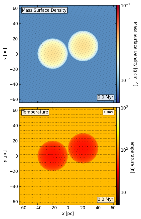
Figure 1: Fiducial initial conditions. Top panel: Mass surface density, shown together with magnetic field structure (gray lines). Bottom panel: Mass-weighted temperature, shown together with the velocity field (black vectors; velocity scale in the top right). GMCs 1 (left) and 2 (right) have identical dimensions with an initial separation of their centers of $2R_{\rm GMC}$ in the $x$-direction and 0 in the $z$-direction. In the $y$-direction, they are offset by an impact parameter $b=0.5R_{\rm GMC}$.

Table 2: Summary of Simulations and Explored Parameter Space

model	name	$v_{\rm rel}$	$B$	$\theta$	$b$
		${\rm km\>s^{-1}}$	(${\rm\mu G}$)	(∘)	($R_{\rm GMC}$)
1	Colliding	10	10	60	0.5
2	Non-Colliding	0	10	60	0.5
3	$v_{\rm rel}=5\>{\rm km/s}$	5	10	60	0.5
4	$v_{\rm rel}=20\>{\rm km/s}$	20	10	60	0.5
5	$\theta=0^{\circ}$	10	10	0	0.5
6	$\theta=30^{\circ}$	10	10	30	0.5
7	$\theta=90^{\circ}$	10	10	90	0.5
8	$b=0R_{\rm GMC}$	10	10	60	0
9	$B=30{\rm\mu G}$	10	30	60	0.5
10	$B=0{\rm\mu G}$, Col.	10	0	-	0.5
11	$B=0{\rm\mu G}$, Non-Col.	0	0	-	0.5

2.2 Numerical Code

We use the numerical code Enzo, a magnetohydrodynamics (MHD) adaptive mesh refinement (AMR) code (Bryan et al., 2014). This code solves the MHD equations using the MUSCL 2nd-order Runge-Kutta temporal update of the conserved variables with the Harten-Lax-van Leer with Discontinuities (HLLD) method and a piecewise linear reconstruction method (PLM). The hyperbolic divergence cleaning method of Dedner et al. (2002) is adopted to ensure the solenoidal constraint on the magnetic field (Wang & Abel, 2008).

For our main results, we use a top level root grid of $128^{3}$ and 3 additional levels of refinement, giving a minimum grid cell size of 0.125 pc and maximum resolution of $1024^{3}$. To test numerical convergence, two additional models of the fiducial colliding case are run at lower resolution. These models have the same $128^{3}$ root grid, but instead have 1 and 2 total levels of AMR, respectively. We perform the equivalent analysis for each resolution case and compare any noteworthy differences in the respective sections.

For all cases, a cell is refined when the local Jeans length becomes smaller than 8 cells. This results in larger volumes of highly refined regions within the GMCs when compared to the 4 cells typically used to avoid artificial fragmentation (i.e., the Truelove criterion; Truelove et al. 1997). However, we note that for our magnetically supported gas the effective “magneto-Jeans mass” will be significantly larger than the thermal Jeans mass. While these refinement conditions do not necessarily capture the full turbulent cascade or dynamo amplification, which would require 30 cells per Jeans length (Federrath et al., 2011), they should nonetheless provide approximations to real GMC structures while sufficiently avoiding artificial fragmentation.

We make use of the “dual energy formalism” that solves the internal energy equation in addition to the total energy equation. This is necessary when thermal energy is dominated by magnetic and kinetic energy, as it is in our case. This method calculates the temperature from the internal pressure when the ratio of thermal to total energy is less than 0.001, and from the total energy otherwise.

We also use a method of limiting the Alfvén speed in order to avoid extremely small timesteps set by Alfvén waves. This was done by setting a magnetic field dependent density floor, determined by a chosen maximum Alfvén velocity, $v_{A}=B/\sqrt{\mu_{0}\rho}=1\times 10^{7}\>{\rm cm\>s^{-1}}$. Thus, for $B\sim 10\>{\rm\mu G}$, only gas at densities below $n_{\rm H}\sim 0.1\>{\rm cm^{-3}}$ is affected by this limit. In our simulations, this corresponds with $\ll 1\%$ of the cells and an even smaller percentage of the total gas mass, thus we determine the overall results to be essentially unaffected.

2.3 Thermal Processes

We are primarily interested in the dense internal structures of GMCs. This gas is almost entirely molecular with densities $n_{\rm H}\gtrsim 10^{2}\>{\rm cm^{-3}}$ and equilibrium temperatures of $\sim 15$ K. For simplicity, we use a constant value of mean particle mass $\mu=2.33\>m_{\rm H}$. We also choose a constant adiabatic index $\gamma=5/3$ throughout the entire simulation domain, following methods adopted in Paper I. While this does not account for the excitation of rotational and vibrational modes of $\rm H_{2}$ that would occur in some shocks, we consider that this is the most appropriate single-valued choice of $\gamma$ for our simulation setup, given our focus on the dynamics of the dense molecular gas.

We implement PDR-based heating and cooling functions that were created and described in detail in Paper I. These functions include atomic and molecular heating and cooling processes in nonequilibrium conditions, taking into account extinction, density, and temperature. Again following Paper I, we assume a FUV radiation field of $G_{0}=4$ (i.e., appropriate for inner Galaxy conditions, e.g., at Galactocentric distances of $\sim 4$ kpc) and background cosmic ray ionization rate of $\zeta=1.0\times 10^{-16}\>{\rm s^{-1}}$. The heating/cooling functions span the density and temperature space of $10^{-3}\geq n_{\rm H}/{\rm cm^{-3}}\geq 10^{10}$ and $2.7\geq T/{\rm K}\geq 10^{7}$ (increasing the upper limits from $10^{6}\>{\rm cm^{-3}}$ and $10^{5}\>{\rm K}$, respectively, from Paper I), encompassing our desired regime of interest and approximating a multi-phase fluid.

The resulting heating and cooling rates are incorporated into Enzo via the Grackle external chemistry and cooling library (Bryan et al., 2014; Kim et al., 2014). The information is read in via the purely tabulated method and modifies the gas internal energy, $E_{\rm int}=p/\left(\gamma-1\right)$, of a given cell with a net heating/cooling rate calculated by

$$H=n_{\rm H}[\Gamma-n_{\rm H}\Lambda]\;\rm erg\,cm^{-3}\,s^{-1},$$ (2)

where $\Gamma$ is the heating rate and $\Lambda$ is the cooling rate.

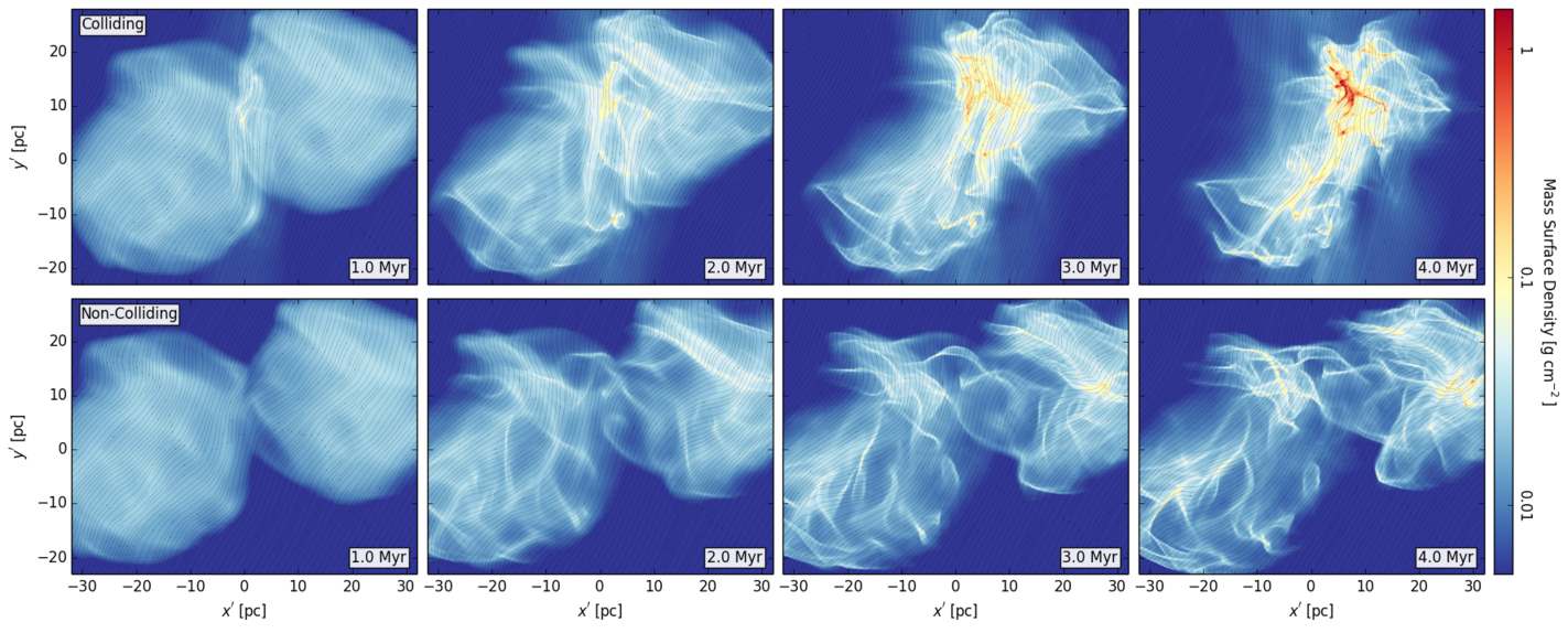
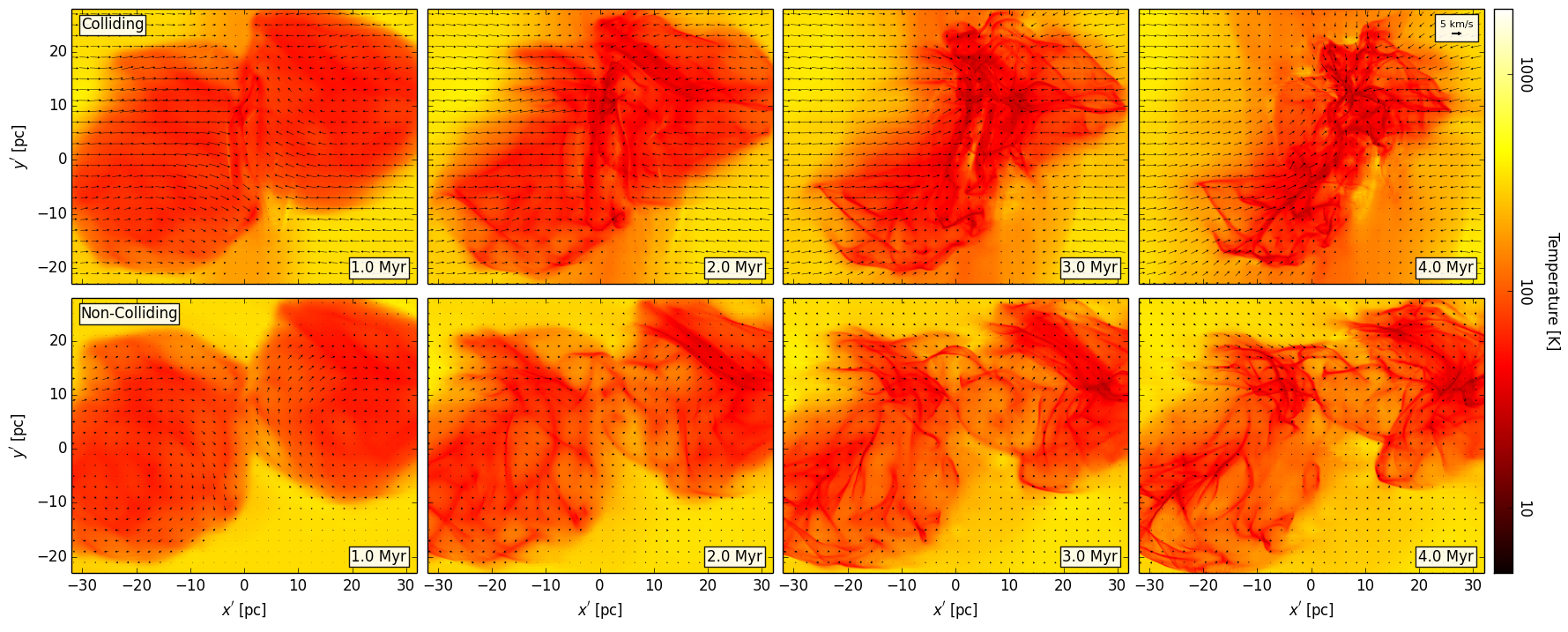
Figure 2: Top: Time evolution of mass surface density for the the fiducial colliding (model 1, 1st row) and non-colliding (model 2, 2nd row) cases. Bottom: Time evolution of mass-weighted temperature for the same models (model 1, 3rd row; model 2 4th row). Snapshots at 1.0, 2.0, 3.0, and 4.0 Myr are shown. Mass-weighted magnetic fields are shown as gray streamlines while velocities are shown as black vectors with the velocity scale shown in the top right.

2.4 Observational Diagnostics

A key output of the aforementioned heating/cooling functions is the detailed information of specific components that contribute to the total heating and cooling rates (see Paper I for the full method). Specifically, by extracting rotational line cooling rates of ¹²CO and ¹³CO, we are able to create synthetic observations of self-consistent CO emissivities via post-processing. Paper I introduced a number of observational diagnostics, namely high-$J$ to low-$J$ CO line intensity ratios and velocity spectra. The analysis in this paper revisits these metrics, but now for 3D geometries and initially turbulent clouds.

We note that while radiative transfer of emissivities is not calculated during post-processing (i.e., we sum contributions along sight lines that is valid in the optically thin limit), it is indirectly incorporated in each cell via the heating/cooling functions. Self-shielding and line optical depths are accounted for in the PDR models, which assume a one-to-one density-extinction relation (see Paper I). Nevertheless, we choose lines in which optical depths should be relatively small. The resulting intensities are simply integrated directly through the simulation domain. We also note that CO freeze-out onto dust grains is not treated in our PDR models. A more detailed study with comparison of our approximate functions to 3D PDR models and radiative transfer calculations is currently in preparation (Bisbas et al., in prep.).

We will present integrated intensity maps and spectra of CO lines and line ratios with rotational excitations $J$=2-1, 3-2, and 8-7 in §3.4 and §3.5, respectively. The dynamical analysis of §3.6 is performed on synthetic ¹³CO($J$=1-0) maps.

3 Results

We perform analysis of the simulations, focusing on the following categories of interest: density and temperature morphologies (§3.1); magnetic field morphologies and strengths (§3.2); mass surface density distributions (§3.3); CO line diagnostics (§3.4); kinematics (i.e., spectra and velocity gradients) (§3.5); and dynamics (i.e., virial analysis) (§3.6).

Primarily, we investigate relative differences between the fiducial colliding and non-colliding cases, with the goal of understanding the physical effects of GMC-GMC collisions and determining potential differentiating observational diagnosis techniques. Additionally, the remaining parameter models are analyzed to supplement the main results by understanding the effects of variations in the collisional parameters.

For visualization and analysis, we often use a rotated coordinate system ($x^{\prime}$,$y^{\prime}$,$z^{\prime}$) relative to the simulation axes ($x$,$y$,$z$) such that $x^{\prime}$,$y^{\prime}$, and $z^{\prime}$ are rotated by the polar and azimuthal angles, respectively, $(\theta,\phi)=(15^{\circ},15^{\circ})$ about each axis. The purpose of this is to remove biases from an artificial collisional plane that develops as a result of our initial conditions of colliding flows of uniform CNM. This plane has negligible dynamical effects on the GMCs, but a magnified observational signature when the line-of-sight is directly aligned along this plane. In some cases, a non-rotated coordinate system denoted by ($x$,$y$,$z$) is sufficiently unaffected by the initial conditions and is thus used for simplicity.

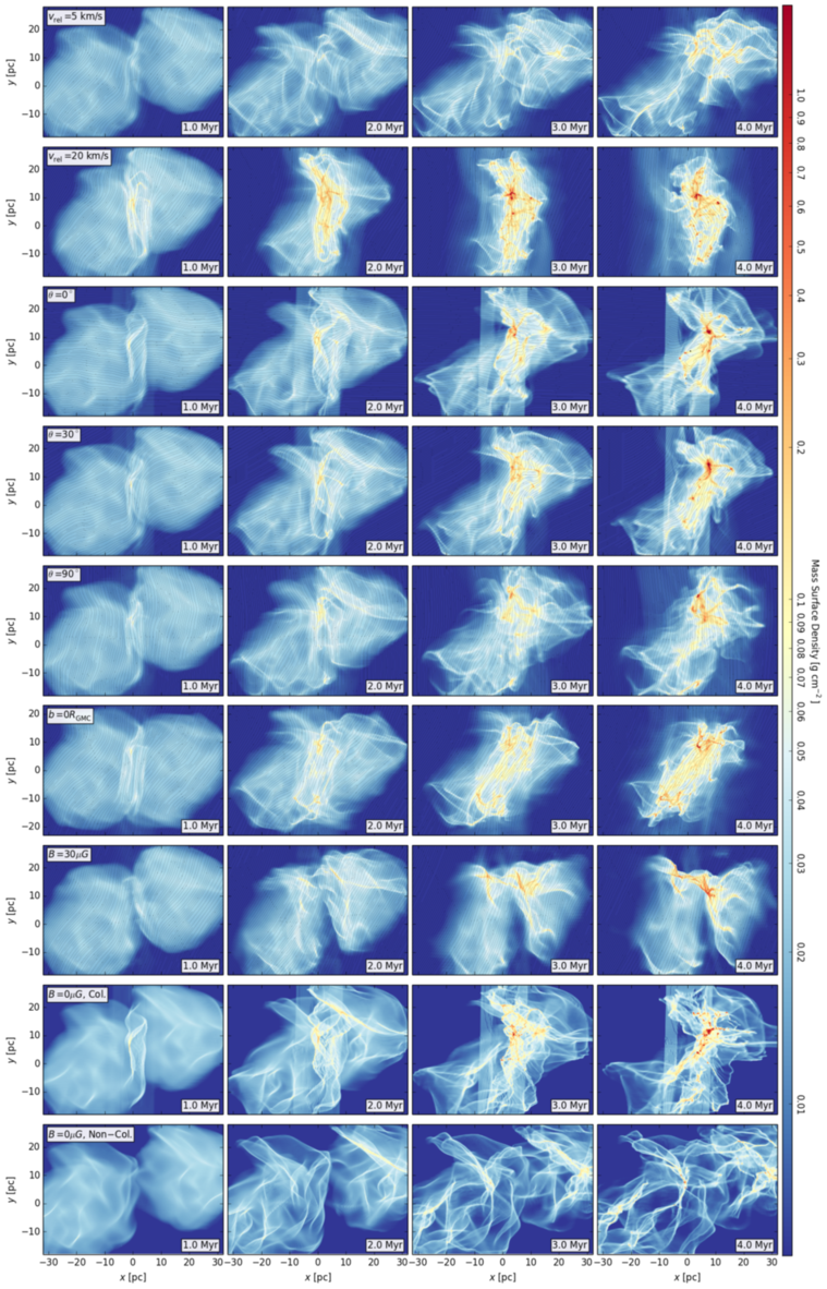
Figure 3: Time evolution of mass surface density for the remaining simulations (models 3 through 11). Each row represents a specific model as labeled, while columns are snapshots at $t$ = 1.0, 2.0, 3.0, and 4.0 Myr are shown. Mass-weighted magnetic fields are represented by gray streamlines.

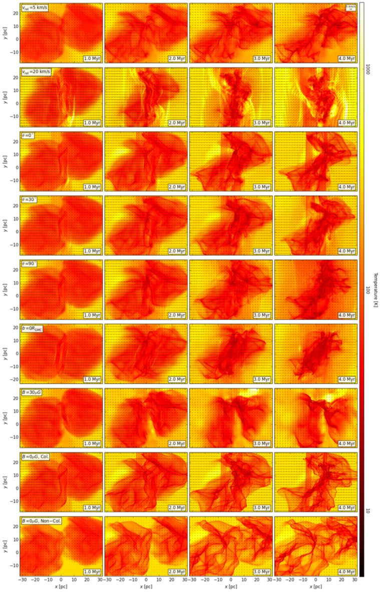
Figure 4: Time evolution of mass-weighted temperature for the remaining simulations (models 3 through 11). Each row represents a specific model as labeled, while columns are snapshots at $t$ = 1.0, 2.0, 3.0, and 4.0 Myr. Mass-weighted velocities are represented by black vectors, with the velocity scale shown in the top right.

3.1 Mass Surface Density and Temperature Morphology

The time evolution of mass surface density (superposed with magnetic field lines) and temperature (superposed with gas velocity vectors) structures in the fiducial colliding and non-colliding cases are shown in Fig. 2. Similar plots for the remaining nine parameter models are shown in Figs. 3 and 4 for density and temperature, respectively.

3.1.1 Fiducial Models

Both the fiducial colliding and non-colliding cases develop filamentary density structures within the GMCs as a result of the turbulent velocity fields. The spatial extent of the non-colliding GMCs is generally retained over the course of $\gtrsim 1$ free-fall time, though the density distribution evolves from an initially uniform density to a network of relatively slowly growing filaments and with increasing differentiation in densities.

For the colliding case, an elongated filamentary sheet-like structure of much higher density quickly develops near the colliding region, with both GMC material and CNM gas being swept up in the large shocks created by the colliding flows. A primary filamentary region results, generally lying in the plane oriented perpendicular to the collision axis, with smaller filaments extending outward. Structures with mass surface densities exceeding $1\>{\rm g\>cm^{-2}}$ are more localized and form at fractions of the original $t_{\rm ff}$, much more quickly relative to the non-colliding case.

The mass surface density structure and magnetic fields mutually affect one another. In the non-colliding case, the densest filaments are qualitatively preferentially aligned perpendicular to magnetic field lines. Additionally, the turbulent material drags the magnetic fields with it, creating twisted and more complex magnetic structures from an initially uniform geometry. In the colliding case, the large-scale flows compress the magnetic fields into the plane perpendicular to the collision axis, effectively re-orienting the magnetic fields in a new locally dominant direction. Relative orientations between mass surface density structure and magnetic fields may be an observable differentiating factor between relatively isolated turbulent GMCs and those which have undergone a major binary collision. A more detailed analysis quantifying these relative orientations is discussed in §3.2. The strong coupling between magnetic field and density in the simulations is expected from flux-freezing in ideal MHD. Non-ideal MHD effects such as ambipolar diffusion may become dominant in certain regimes within the GMCs and will be explored in a subsequent paper.

The PDR-based heating/cooling functions (described in §2.3 and Paper I) enable us to approximate the thermal behavior of gas in the atomic-to-molecular regime and model non-equilibrium effects, specifically shocks. For both models, the temperature is generally near the equilibrium temperature for the particular density: $\sim$ tens of Kelvin at $n_{\rm H}>100\>{\rm cm^{-3}}$ and $\sim 10^{2}$ K to $10^{3}$ K for $n_{\rm H}\lesssim 10\>{\rm cm^{-3}}$. In the non-colliding case, the deviation of actual gas temperature from the equilibrium temperature curve is generally small. In the colliding case, large shock waves are created, resulting in a high-temperature shock front that sweeps through GMC material as it enters the post-shock region. Upon doing so, a central region of low temperature filamentary gas develops, again strongly correlating with density structures. This region of $T\sim 15\>{\rm K}$ gas grows in size as more dense material accumulates.

3.1.2 Parameter Models

Next, we discuss how variations in the collision parameters affect the morphologies of mass surface density and temperature through their subsequent evolution. Figs 3 and 4 provide a direct comparison between these models.

Collision velocities of $v_{\rm rel}=5$ and 20 km/s are explored in models 3 and 4, respectively. By $t=4\>{\rm Myr}$, Model 3 has not yet produced gas of $\Sigma>1\>{\rm g\>cm^{-2}}$ but contains morphological features somewhat in between the non-colliding and colliding fiducial models. A relatively dense filament can be seen forming in the central collision region, while a separate region within GMC 2 has begun to form a second dense filament. Both regions correspond spatially with dense structures that form in the non-colliding case, which points to turbulence as the dominant formation mechanism, but their densities are further enhanced at earlier times due to the collision. These regions are also sites of the lowest temperatures, cooling to $\sim 15\>{\rm K}$. Model 4 creates a stronger shock, higher-density collision region, and higher-density clumps at earlier times. The main filamentary sheet appears more localized to the central collision region, and many dense core-like structures are created along the length of this general filament relative to the fewer, more elongated structures created in more slowly colliding cases. The higher collision velocity also created high-temperature ($T>1000\>{\rm K}$) shock fronts propagating anti-parallel to the incoming flow as well as oblique shocks created at the GMC boundaries corresponding to the impact parameter.

Initial magnetic field orientations of $\theta=0^{\circ}$, $30^{\circ}$, and $90^{\circ}$ are explored in models 5, 6, and 7, respectively. As magnetic pressure acts in directions perpendicular to the field lines, it is expected that smaller values of $\theta$ should result in less inhibited flow and yield higher density gas. While turbulence does stir up the magnetic field lines, the larger-scale uniform direction and bulk flow dominate the resulting morphology. Thus, higher density gas is formed at earlier times for smaller $\theta$, with the extent of general GMC substructures greatest along the direction of the large-scale magnetic fields. The temperatures within the dense regions are near equilibrium, aside from regions through which shocks are actively crossing. Among these models, ambient gas near the collisional region exhibit differences in the temperature morphology due to the density of post-shock material. More perpendicular values of $\theta$ result in post-shock regions with densities spread over larger extents created by built-up magnetic pressure from the flows; this produces growing regions of $T\sim 100\>{\rm K}$ gas surrounding the GMC material.

Model 8 explores the effects of a head-on collision ($b=0$). Compared to the fiducial colliding case, the head-on collision produces fairly similar structures in density and temperature, though the features exhibit greater morphological symmetry: dense, cold clumps and filaments are created at both positive and negative y-values as opposed to predominantly positive y-values for the $b=0.5R_{\rm GMC}$ cases.

Model 9 explores a case of stronger magnetic field, with $B=30\>{\rm\mu G}$, resulting in GMCs with a mass-to-flux ratio $\lambda_{\rm GMC}=1.43$, only slightly magnetically supercritical, and CNM with $\lambda_{0}=0.5$, distinctly magnetically subcritical. This threefold increase in magnetic field strength, however, creates roughly an order of magnitude increase in magnetic pressure ($P\propto B^{2}$.) The final result is an evolution in which the clouds are compressed by the bulk flows, but merging is inhibited. The resulting filaments still accumulate towards the central colliding region but are more dispersed than in the fiducial case.

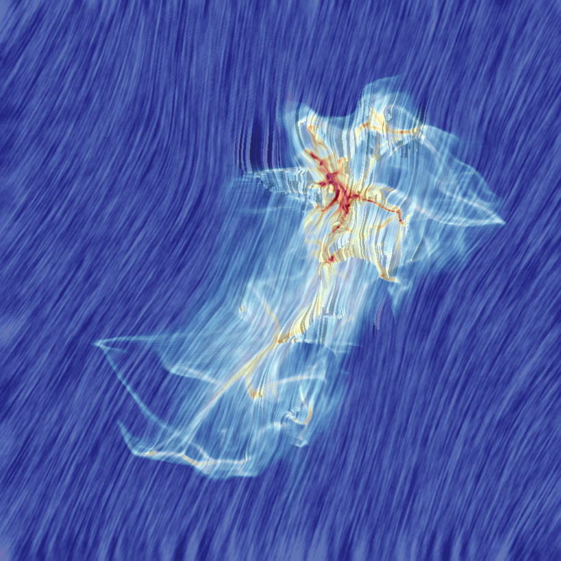
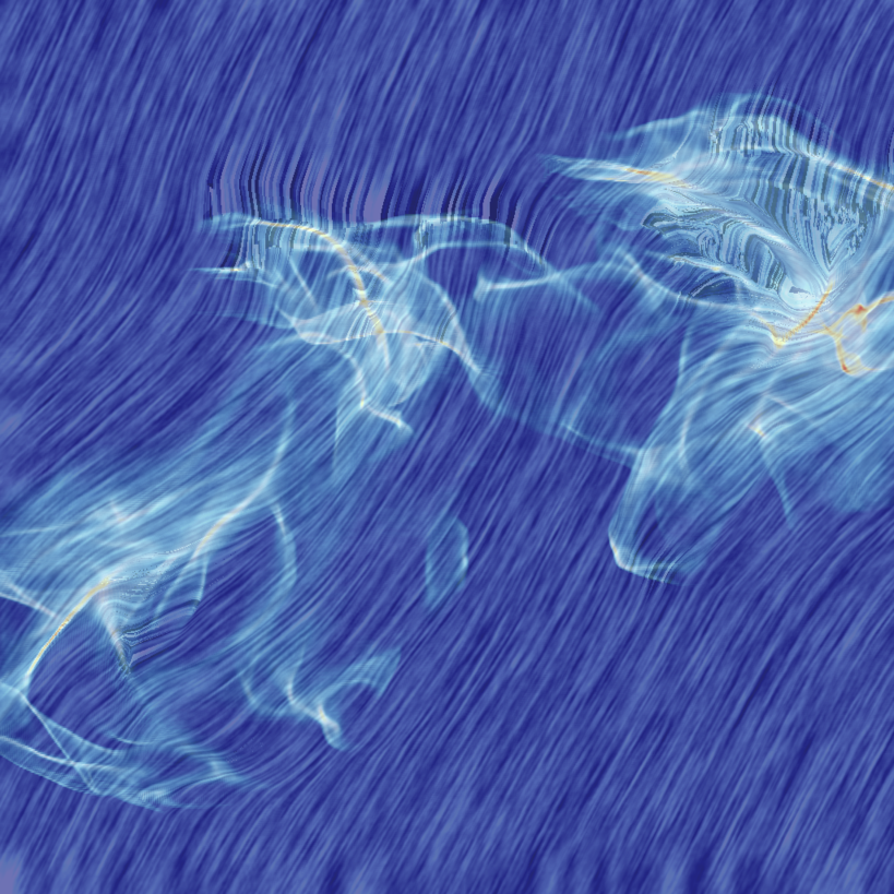
Figure 5: Visualization of mass surface density and projected magnetic field polarization vectors for (left) the fiducial colliding and (right) non-colliding simulations. Mass surface density is represented by the underlying colors, while the magnetic fields are ”painted” along their polarization direction using the LIC method. The domain shown represents a physical projected area of $64~{}{\rm pc}^{2}$.

Unmagnetized cases are explored in models 10 and 11, the respective colliding and non-colliding simulations. In both models, deviations in density structures arise quickly in the evolution as there are fewer forces inhibiting collapse. Denser filaments form more quickly, which in turn collapse into clump-like structures on the order of $t_{\rm ff}$. The collision acts to localize the resulting clumps in the central region, while the non-colliding clouds form clumps at fairly evenly spatially distributed regions throughout each parent cloud. The density and temperature contrasts are sharper for the non-magnetized clouds, compared to the smoother, more connected structures of the magnetized cases.

A more detailed quantitative analysis investigating mass surface density distribution and evolution using probability distribution functions (PDFs) is discussed in §3.3.

3.2 Magnetic Fields

Interstellar magnetic fields and their complex interactions with both turbulence and gravity likely play an important role in the formation and evolution of GMCs, filaments, and eventually stars. However, their dynamical importance is not well-determined.

Two important magnetic field parameters that influence gas dynamics are magnetic field orientation and strength. Observationally, the projected magnetic field orientation averaged along the line-of-sight can be studied via dust polarization maps (assuming a particular grain alignment model), while the line-of-sight component of the magnetic field strength can be calculated from molecular line splitting due to the Zeeman effect.

Recently, the ability to understand magnetic field orientations in Galactic molecular clouds has been greatly expanded by the Planck space observatory, with its all-sky capability of measuring both dust polarization and optical depth, and resolution to probe the interiors of nearby ($d<450\>{\rm pc}$) clouds (see Planck Collaboration et al. (2016, hereafter PlanckXXXV)).

From our simulations incorporating magnetized turbulence on the GMC-scale, we can perform similar types of analysis in order to better understand observable magnetic field signatures and their connections with underlying physical processes. We first analyze magnetic field orientation relative to mass surface density structures and then investigate magnetic field strength relative to gas volume density. Fig. 5 uses the line integral convolution (LIC, first proposed by Cabral & Leedom 1993) method to combine visualization of column density and projected magnetic field structure for the fiducial colliding and non-colliding cases.

3.2.1 Relative Orientations: $B$ vs. iso-$N_{\rm H}$

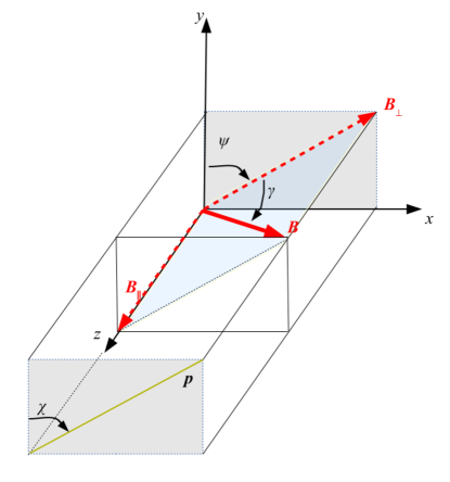
Figure 6: Diagram of angle definitions. For a magnetic field $\bm{B}$ and an observer viewing along the -$z$ axis, $\gamma$ is the inclination angle between $\bm{B}$ and the plane-of-sky, while $\psi$ is the position angle between $\bm{B}_{\perp}$ (the plane-of-sky magnetic field component) and the “north” direction (in this case, $y$). The integrated polarization pseudo-vector yields an angle $\chi$.

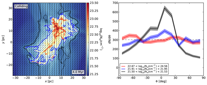
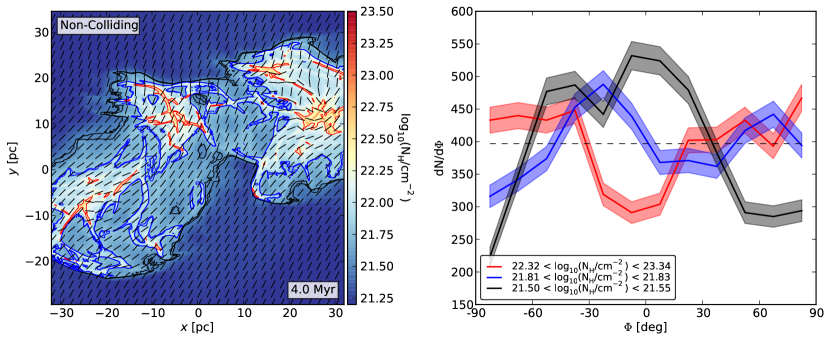
Figure 7: Left panels: Column density maps, $\log_{10}(N_{\rm H}/\rm{cm^{-2}})$, with black vectors representing the normalized plane of sky polarization field. The colliding case is shown in the top figure, while the non-colliding case is in the bottom figure. Right panels: Histograms of Relative Orientations (HROs) comparing the angle between the polarization pseudo-vector $p$ vs. iso-$N_{\rm H}$ contours pixel-by-pixel in the fiducial colliding (top) and non-colliding (bottom) simulations. The projected map is divided into 25 column density bins of equal pixel count. HROs for the lowest (1st bin; black), middle (12th bin; blue), and highest (25th bin; red) $N_{\rm H}$ bin are shown, using angle bins of $15^{\circ}$. The histogram color corresponds with the colored contours that bound low (black), intermediate (blue), and high (red) column density regions of the projection map. Histograms with peaks at $0^{\circ}$ correspond to $p$ predominantly aligned with iso-$N_{\rm H}$ contours (i.e., $B$-fields aligned along filaments). Histograms with peaks at $\pm 90^{\circ}$ correspond to $p$ predominantly perpendicular to iso-$N_{\rm H}$ contours (i.e., $B$-fields aligned perpendicular to filaments).

To study magnetic field orientations, we utilize the Histogram of Relative Orientations (HRO, Soler et al. 2013). The HRO is a statistical tool that quantifies the magnetic field orientation relative to the gradient of the column density. It can be performed on polarization observations (e.g., PlanckXXXV) as well as numerical simulations (e.g., Planck Collaboration et al., 2015; Chen et al., 2016) to study the mutual dependence of magnetic fields on density structures.

The HRO investigates the angle $\phi$ between the polarized emission $\bm{p}$ and $N_{\rm H}$ iso-contours (orthogonal to $\nabla N_{\rm H}$):

$$\phi=\arctan\left(\frac{\nabla N_{\rm H}\cdot\bm{p}}{|\nabla N_{\rm H}\times\bm{p}|}\right)$$ (3)

$\bm{p}$ is a pseudo-vector defined by

$$\bm{p}=(p\sin\chi)\hat{\bm{x}}+(p\cos\chi)\hat{\bm{y}}$$ (4)

where $p$ is the polarization fraction and $\chi$ is the polarization angle. Thus, one can think of $\phi$ also as being the relative angle between the magnetic field and the filamentary axis of structures seen in mass surface density maps. Note that the convention we adopt for $\phi$ follows PlanckXXXV but is shifted $\pi/2$ from that defined in Soler et al. (2013) and Chen et al. (2016).

We assume a constant polarization fraction $p=0.1$ (though Planck Collaboration et al. (2015) and Chen et al. (2016) use various grain polarization fraction models in their analysis) while $\chi$ is the polarization angle derived from the Stokes parameters.

The relative Stokes parameters can be calculated following previous work (Lee & Draine, 1985; Fiege & Pudritz, 2000; Kataoka et al., 2012; Chen et al., 2016):

$$q=\int n\cos 2\psi\cos^{2}\gamma ds$$ (5)

$$u=\int n\sin 2\psi\cos^{2}\gamma ds$$ (6)

where $\gamma$ is the angle between the local magnetic field relative to the plane of the sky, while $\chi$ is the angle of the magnetic field on the plane of the sky relative to the “north” axis (see Fig.  6). For a coordinate orientation where the $y$-axis can be defined as “north” with the line of sight directed along the $z$-axis, the relative Stokes parameters can be written as (see Chen et al. (2016)):

$$q=\int n\frac{B_{y}^{2}-B_{x}^{2}}{B^{2}}ds$$ (7)

$$u=\int n\frac{2B_{x}B_{y}}{B^{2}}ds$$ (8)

Finally, we can calculate $\chi$, the polarization angle on the plane of the sky:

$$\chi=\frac{1}{2}\arctan 2(u,q)$$ (9)

where $\arctan 2$ is the arctangent function with two arguments, returning angles within $[-\pi,\pi]$ based on the quadrant of the inputs.

To distinguish cloud structure from background structure, PlanckXXXV selected pixels in regions where the magnitude of the column density gradient exceeded the mean gradient of a reference diffuse background field. In our case, the gradient threshold was chosen to be 0.25 the average value of the fiducial colliding case in order to better capture the GMC material. We apply this value for each case and additionally apply a cut of the lowest column density values ($N_{\rm H}<21.5\>{\rm cm^{2}}$). (Note: we assume $n_{\rm He}=0.1n_{\rm H}$, giving a mass per H of $2.34\times 10^{-24}\>{\rm g}$.) $\phi$ is then calculated for each remaining pixel in the projected domain. This domain is divided into 25 bins of $N_{\rm H}$ ranges, each containing an equal number of pixels. For a given $N_{\rm H}$ range, an HRO plot can be created, comparing the distribution of cells for each angle $-90^{\circ}<\phi<90^{\circ}$. We create HROs for the lowest, intermediate, and highest column density bins to investigate how the magnetic field orientation changes as a function of column density. This means histograms peaking at $\phi=0^{\circ}$ correspond to $\bm{p}$ mostly aligned parallel to filamentary structure, while peaks at $\phi=\pm 90^{\circ}$ correspond to perpendicular alignment of magnetic fields with filaments.

The left-hand column of Fig. 7 shows column density maps of the fiducial colliding and non-colliding cases over-plotted with magnetic field vectors and colored contours defining the three aforementioned $N_{\rm H}$ ranges. The right-hand column shows the respective HROs, representing material within the specific column density range. In the fiducial colliding case, the HRO peaks near $0^{\circ}$ especially for the low column density bins, while the intermediate and high column density bins show slight preference to this value. This signifies a predominantly parallel alignment of $\bm{p}$ with iso-$N_{\rm H}$ contours for the colliding case. Likewise, the fiducial non-colliding case exhibits strong peak near $0^{\circ}$ for the low column density bin, but is roughly flat for moderate column densities while peaking at $\phi=\pm 90^{\circ}$ for the highest column densities. This signifies a shift from predominantly parallel alignment of $\bm{p}$ with iso-$N_{\rm H}$ contours at low densities to a predominantly perpendicular alignment at high densities.

In order to distinguish trends along the entire column density range and compare models with various collisional parameters, we further quantify HROs using the histogram shape parameter $\xi$, which is defined as (see Soler et al. (2013) and PlanckXXXV):

$$\xi=\frac{A_{\rm c}-A_{\rm e}}{A_{\rm c}+A_{\rm e}},$$ (10)

where $A_{c}$ is the area within the central region ($-22.5^{\circ}<\phi<22.5^{\circ}$) under the HRO, while $A_{e}$ is the area within the extrema ($-90^{\circ}<\phi<-67.5^{\circ}$ and $67.5^{\circ}<\phi<90^{\circ}$) of the HRO. Thus $\xi$ is independent of total bin number and normalizes relative differences within the individual histogram. $\xi>0$ is indicative of a concave histogram ($\bm{p}$ preferentially parallel to iso-$N_{\rm H}$ contours), while $\xi<0$ is indicative of a convex histogram ($\bm{p}$ preferentially perpendicular to $N_{\rm H}$).

From PlanckXXXV, uncertainties in the HROs were found to be dominated by histogram binning, which we include in our analysis here. The $k$th bin in the histogram has variance

$$\sigma_{k}^{2}=h_{k}\left(1-\frac{h_{k}}{h_{\rm tot}}\right)$$ (11)

with $h_{k}$ and $h_{\rm tot}$ being the number of samples in the $k$th bin and total number of samples, respectively. The total uncertainty of $\xi$, given by $\sigma_{\xi}$, is then calculated from

$$\sigma_{\xi}^{2}=\frac{4(A_{\rm e}^{2}\sigma_{A_{\rm c}}^{2}+A_{\rm c}^{2}\sigma_{A_{\rm e}}^{2})}{(A_{\rm c}+A_{\rm e})^{4}}.$$ (12)

Also following PlanckXXXV, we can study trends in $\xi$ vs $\log_{10}(N_{\rm H}/{\rm cm^{2}})$ by fitting a linear function

$$\xi=C_{\rm HRO}[\log_{10}(N_{\rm H}/{\rm cm^{2}})-X_{\rm HRO}].$$ (13)

$C_{\rm HRO}$ and $X_{\rm HRO}$ can be used as quantitative parameters to compare general relationships between all the simulation models. A negative slope $C_{\rm HRO}$ represents $\bm{p}$ becoming more parallel with filaments as $N_{\rm H}$ increases, while a positive $C_{\rm HRO}$ would signify an increasingly perpendicular relative orientation. $X_{\rm HRO}$ represents the crossover value of $N_{\rm H}$ at which $\bm{p}$ switches from perpendicular to parallel to iso-$N_{\rm H}$ contours.

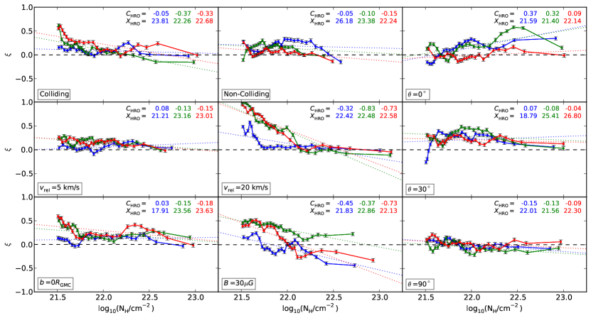
Figure 8: Comparison of the histogram shape parameter, $\xi$, vs column density, $N_{\rm H}$, among the magnetized simulations. $\xi>0$ represents a preferentially parallel orientation between magnetic field lines and iso-$N_{\rm H}$ contours, while $\xi<0$ represents a preferentially perpendicular orientation. The blue, green, and red lines represent lines of sight from the $x^{\prime}$,$y^{\prime}$, and $z^{\prime}$ axes, respectively. The parameters $C_{\rm HRO}$ and $X_{\rm HRO}$ for the best linear fit for each line of sight are indicated in the respective color.

Figure 8 shows $\xi$ vs. $N_{\rm H}$ for our magnetized runs (models 1-9). This relation does not appear to have strong dependence on line of sight, agreeing fairly well for each model along the $y^{\prime}$ and $z^{\prime}$ viewing directions. Viewing from the $x^{\prime}$-direction does result in occasional deviations, but for the most part it is well-correlated. These models are generally fit with $C_{\rm HRO}<0$ and $X_{\rm HRO}\approx 22$, which agree with the observational results from Planck Collaboration et al. (2016). From the 10 molecular clouds in their study, mean values of $C_{\rm HRO}=-0.41$ and $X_{\rm HRO}=22.16$ were found, with uncertainties in $\xi$ generally in the tens of percent range.

However, between the various models themselves, there are notable differences. The fiducial non-colliding case has a fairly flat slope, with $C_{\rm HRO}\approx-0.1$ and $X_{\rm HRO}\approx 23.9$. In comparison, the fiducial colliding case has a steeper slope, with $C_{\rm HRO}\approx-0.3$, and a slightly lower intercept, $X_{\rm HRO}\approx 22.9$. The linear fits to both fiducial models are similarly consistent. The physical interpretation is that the collision influences the overall preferential alignment of magnetic fields relative to gas filaments, specifically driving the value of $\xi$ more positive for lower column structures (i.e., more concave HRO; $\bm{p}$ preferentially parallel to low $N_{\rm H}$), and more negative for higher column structures (i.e., more convex HRO; $\bm{p}$ preferentially perpendicular to high $N_{\rm H}$).

This is emphasized when varying collisional velocities are explored (models 3 and 4). The intermediate collision velocity ($v_{\rm rel}=5\>{\rm km/s}$) results in a slight increase in $C_{\rm HRO}$, while the high collision velocity ($v_{\rm rel}=20\>{\rm km/s}$) increases the slope strongly, with $C_{\rm HRO}$ as steep as -0.83. The value of $\xi$ seems most affected at low $N_{\rm H}$, while staying relatively steady at $\xi\lessapprox 0$ for high $N_{\rm H}$. The $x^{\prime}$ line-of-sight in this case does not capture much of the effect of the collision on the magnetic field polarization.

The effects of initial magnetic field orientation (models 5, 6, and 7) are less direct, but initial orientation appears to primarily influence the value of $C_{\rm HRO}$, with $\theta=0^{\circ}$ resulting in positive $C_{\rm HRO}$.

A head-on collision (model 8) appears to have a small effect on the overall $\xi$ vs $N_{\rm H}$ relation when compared to the fiducial colliding model. There is a slight upward shift in values of $X_{\rm HRO}$, but the overall shape is generally similar. The impact parameter, while significant on the GMC scale, would not be expected to greatly influence the behavior of collisions between smaller individual substructures that determine the local B-field polarization.

Lastly, the stronger-field case of $B=30\>{\rm\mu G}$ (model 9) has notable effects on the slope, with $C_{\rm HRO}=-0.73$ in the $z^{\prime}$ line of sight, as well as a moderate crossover point $X_{\rm HRO}\approx 22$. This model produces the most preferentially perpendicular alignment of B-field and filamentary structure at high $N_{\rm H}$.

The resolution analysis of HRO results yielded similar values for all lines of sight in the fiducial colliding model, with signs of convergence when increasing resolution from 1-2 AMR levels to 2-3.

HROs and subsequent histogram shape parameter analysis may be a useful tool for differentiating between non-colliding and colliding clouds given the strong correlations with collision velocity and B-field strength and, to a lesser extent, various other collisional parameters.

3.2.2 Magnetic Field Strengths: $|B|$ vs. $n_{\rm H}$

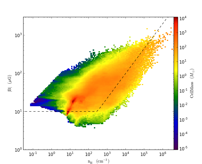
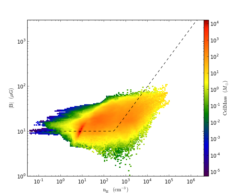
Figure 9: Phaseplots examining $|B|$ vs. $n_{\rm H}$ for (left) the fiducial colliding and (right) non-colliding simulations at $t=4.0\>{\rm Myr}$. The colorbar displays the total gas mass at each point. The dashed line represents the “Crutcher relation,” where $B_{\rm max}=B_{0}=10~{}{\rm\mu G}$ for $n_{\rm H}<300\>{\rm cm^{-3}}$ and $B_{\rm max}=B_{0}(n_{\rm H}/300\>{\rm cm^{-3}})^{2/3}$ otherwise. The cutoff in the low density regions is due to the Alfvén limiter.

The magnetic field strength as a function of density in GMCs is another property that is potentially important for the evolution of substructure. Figure 9 explores the $|B|$ vs. $n_{\rm H}$ relation for the fiducial colliding and non-colliding GMCs. The colliding case involves creation of regions of both high density and higher magnetization than the non-colliding case. The majority of the overall gas mass remains near the initialized values of $B$ and $n_{\rm H}$, but the collision generally produces stronger field strengths for a given density. The concentration of gas mass from $10<n_{\rm H}/{\rm cm^{-3}}<100$ corresponds primarily with the ambient gas accumulating in the collision region, where the initial magnetic field is similarly compressed. In the non-colliding case, the gas mass mostly stays concentrated near the initialized levels, with especially the ambient, CNM gas evolving in a mostly quiescent manner.

Although our simulations are initialized with relatively idealized conditions, both fiducial models develop a $B$ vs. $n_{\rm H}$ behavior approximately consistent at least in general shape with the “Crutcher relation” (Crutcher et al., 2010) where $B_{\rm max}=B_{0}=10~{}{\rm\mu G}$ for $n_{\rm H}<300\>{\rm cm^{-3}}$ and $B_{\rm max}=B_{0}(n_{\rm H}/300\>{\rm cm^{-3}})^{2/3}$, for $n_{\rm H}>300\>{\rm cm^{-3}}$. Our models exhibit relatively stronger $|B|$ overall, exceeding the maximum values statistically determined by observations comprising the relation. The gas in the colliding case reaches ${\rm mG}$ strengths at $n_{\rm H}\approx 10^{6}\>{\rm cm^{-3}}$ as the accumulation of gas to higher densities in turn compresses the magnetic fields along with it. The lower envelope of the phaseplot appears to exhibit a slight elbow near $10^{3}\>{\rm cm^{-3}}$ in both the colliding and non-colliding cases. This is roughly consistent with the Crutcher relation, although it is important to note that the elbow occurs in the upper envelope of the Crutcher data. The gas near this range retains roughly constant values of $|B|$ in the tens of ${\rm\mu G}$ range. The non-colliding case also exhibits a similar lower envelope relation, with a smaller overall range in density and $|B|$.

Deviations exist between $|B|$ found in our models and the maximum $|B|$ statistically predicted from observations, particularly in the highly magnetized, low-density gas of the colliding case. However, this may be attributable to the particular choice of our initial field strengths and other simulation parameters.

3.3 Mass Surface Density Probability Distribution Functions

PDFs of mass surface density (or $N_{\rm H}$ or $A_{\rm V}$) have been used as tools to study the physical characteristics of observed molecular clouds and IRDCs (e.g. Kainulainen et al., 2009; Kainulainen & Tan, 2013; Butler et al., 2014). Mechanisms such as turbulence, self-gravity, shocks, and magnetic fields all contribute to the resulting distribution of $\Sigma$.

For turbulent clouds, the $\Sigma$-PDF is generally characterized as log-normal at lower $N_{\rm H}$ ranges, while at higher $N_{\rm H}$ an additional power law tail component is often measured and attributed to compression due to self-gravity. The width of the log-normal component is expected to correlate with the strength of turbulence, i.e., the Mach number of typical shocks. The fraction of mass in the high-$\Sigma$ power law tail may correlate with the degree of gravitational instability and the efficiency of star formation.

We present area ($p_{A}(\Sigma)$) and mass-weighted ($p_{M}(\Sigma)$) PDFs of $(32\>{\rm pc})^{3}$ extracted regions projected along the $z^{\prime}$-direction through each of our models. For each distribution, we also find the best-fit log-normal function:

$$p(\Sigma)=\frac{A}{(2\pi)^{1/2}\sigma_{\ln\Sigma}}\exp{\left[-\frac{(\ln\Sigma-\overline{\ln\Sigma})^{2}}{2\sigma_{\ln\Sigma}^{2}}\right]}$$ (14)

where $\sigma_{\ln\Sigma}$ is the standard deviation of $\ln\Sigma$. A scale factor $A$ is included to allow for adjustment between differing PDF normalization schemes. A summary of the fit parameters for each run is shown in Table 3.

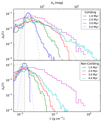
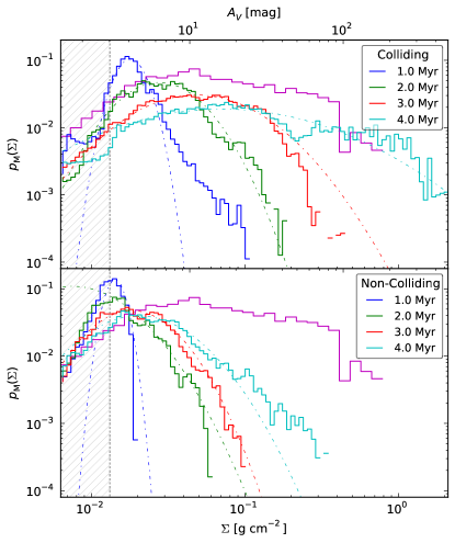
Figure 10: Area-weighted (left column) and mass-weighted (right column) $\Sigma$-PDFs of $(32\>{\rm pc})^{3}$ regions from the fiducial colliding (top) and non-colliding (bottom) cases as they evolve in time. $\Sigma$-PDFs for each case at $t$=1.0, 2.0, 3.0, and 4.0 Myr are shown in blue, green, red, and cyan, respectively. The best log-normal fits for each case are plotted as dash-dotted lines of the same color. In each panel, the $\Sigma$-PDFs from observations of a massive IRDC from Lim et al. (2016) is shown in magenta. The shaded region denotes areas of $A_{V}<3\>{\rm mag}$, matching the completeness levels the observed IRDCs.

Figure 10 shows the time evolution of area and mass-weighted $\Sigma$-PDFs for the fiducial colliding and non-colliding cases. For each case, the region is centered on the position of maximum $\rho$ at the respective 4 Myr timestep to capture the evolution of the dense filament.

As the region evolves, both cases exhibit a broadening of the distribution, with $\sigma_{\ln\Sigma,A}$ increasing over 3 Myr from 0.200 to 1.079 for colliding clouds and 0.143 to 0.600 for non-colliding clouds. Likewise, $\sigma_{\ln\Sigma,M}$ increases from 0.215 to 1.413 (colliding) and 0.142 to 0.691 (non-colliding). The values for $\overline{\Sigma}_{A}$ stay relatively constant, with slight increases for the colliding case. $\overline{\Sigma}_{M}$ increases for both cases, with a much stronger increase in the colliding case due to the high densities created.

Both the area and mass-weighted $\Sigma$-PDFs are generally well-fit with a single log-normal, though the colliding case at 1.0 Myr and 4.0 Myr and non-colliding case at 4.0 Myr exhibit slight excesses at the high-$\Sigma$ end.

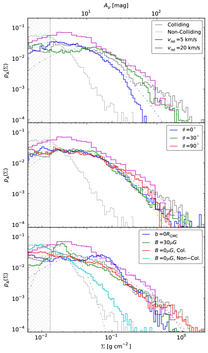
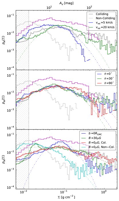
Figure 11: Area-weighted (left column) and mass-weighted (right column) $\Sigma$-PDFs of $(32\>{\rm pc})^{3}$ regions from the parameter models for each category of (top) $v_{\rm rel}$, (middle) $\theta$, and (bottom) $|B|$ and $b$. $\Sigma$-PDFs for each case at $t=4\>{\rm Myr}$ are shown The fiducial colliding and non-colliding cases at $t=4\>{\rm Myr}$ are plotted in dark and light gray, respectively, for reference in each figure. The best log-normal fits for each case are plotted as dash-dotted lines of the same color. In each panel, the $\Sigma$-PDFs from observations of a massive IRDC from Lim et al. (2016) is shown in magenta and the shaded region denotes areas of $A_{V}<3\>{\rm mag}$, matching the completeness levels the observed IRDCs.

In Figure 11, we calculate area and mass-weighted $\Sigma$-PDFs for the parameter models at $t=4\>{\rm Myr}$. The regions are centered at the position of maximum $\rho$ in each case. The figures are organized by models comparing collision velocity (models 3, 4), magnetic field direction (5, 6, 7), and impact parameter (8) and magnetic field strength (9), respectively. The fiducial colliding and non-colliding cases are also included for reference in each figure.

The greatest differences arise from the collision velocity. Higher values of $v_{\rm rel}$ create greater relative amounts of gas at both high and low mass surface densities, resulting in increasingly higher values of $\sigma_{\ln\Sigma_{A}}$ and $\sigma_{\ln\Sigma_{M}}$. $\overline{\Sigma}_{A}$ and $\overline{\Sigma}_{M}$ also show monotonic increases with collision velocity.

An inspection of initial magnetic field orientation yields fairly similar $\Sigma$-PDFs and corresponding PDF parameters for each case. Thus, although the variation of $\theta$ leads to quite different density and temperature morphologies, the resulting $\Sigma$-PDFs are much less affected.

The variation of $b$ and $|B|$ resulted in insignificant changes to the $\Sigma$-PDFs, though the unmagnetized colliding case reached the highest mass surface densities. However, the PDF parameters for each of these colliding cases are relatively similar. When compared with the unmagnetized, non-colliding, case, the differences in $\Sigma$-PDFs due to collision velocity are emphasized further.

Butler et al. (2014) and Lim et al. (2016) have presented the $\Sigma$-PDF of a 30 pc scale region centered on a massive IRDC that is embedded in a GMC. Near+mid infrared extinction mapping and sub-mm dust continuum emission methods have been used to derive the PDF. The region contains a minimum close contour of $\Sigma=0.013\>{\rm g\>cm^{-2}}$ ($A_{V}=3$ mag), so is expected to be complete for higher values of $\Sigma$. The area-weighted PDF (weighting by the total area of those pixels with $A_{V}\geq 3$ mag) is well fit by a single log-normal with $\overline{\Sigma}_{A}=0.039\>{\rm g\>cm^{-2}}$ and $\sigma_{\ln\Sigma,A}=1.4$. There is a relatively limited fraction of material at high $\Sigma$’s in excess of the log-normal, i.e., $\epsilon_{\rm pl}\lesssim 0.1$. These features are quite similar to some of the simulated PDFs, especially the colliding case at 4 Myr, which is well-fit with $\overline{\Sigma}_{A}=0.021\>{\rm g\>cm^{-2}}$ and $\sigma_{\ln\Sigma,A}=1.1$. The $v_{\rm rel}=20\>{\rm km\>s^{-1}}$, $\theta=0^{\circ}$ and $b=0R_{\rm GMC}$ models also have similar values. While this does not prove any particular scenario, the colliding cases in general demonstrate strong consistency with observations.

In studying resolution effects, the $\Sigma$-PDFs are well-converged, with histogram noise decreasing as resolution increases and overall values of log-normal fit parameters in agreement within a few percent.

Table 3: Properties of $\Sigma$-PDFs

name	$\sigma_{\ln\Sigma,A}$	$\overline{\Sigma}_{A}$	$\sigma_{\ln\Sigma,M}$	$\overline{\Sigma}_{M}$
		(${\rm g\>cm^{-2}}$)		(${\rm g\>cm^{-2}}$)
Colliding (1.0 Myr)	0.200	0.017	0.215	0.018
Colliding (2.0 Myr)	0.567	0.020	0.539	0.028
Colliding (3.0 Myr)	0.850	0.023	0.835	0.048
Colliding (4.0 Myr)	1.079	0.021	1.413	0.071
Non-Col. (1.0 Myr)	0.143	0.014	0.142	0.014
Non-Col. (2.0 Myr)	0.503	0.009	0.691	0.008
Non-Col. (3.0 Myr)	0.586	0.013	0.545	0.018
Non-Col. (4.0 Myr)	0.600	0.015	0.691	0.020
$v_{\rm rel}=5$ km/s	1.004	0.016	0.876	0.043
$v_{\rm rel}=20$ km/s	0.986	0.038	0.818	0.086
$\theta=0^{\circ}$	1.045	0.022	0.969	0.061
$\theta=30^{\circ}$	0.893	0.027	0.883	0.058
$\theta=90^{\circ}$	1.255	0.017	1.123	0.077
$b=0R_{\rm GMC}$	0.982	0.038	0.610	0.079
$B=30\mu G$	0.407	0.019	1.868	0.027
$B=0\mu G$, Col.	1.317	0.014	1.423	0.070
$B=0\mu G$, Non-Col.	1.007	0.005	1.119	0.013

3.4 Integrated Intensity Maps

From the PDR-based heating and cooling functions, we extract ¹²CO and ¹³CO molecular line cooling information to create self-consistent synthetic integrated intensity maps via post-processing. ¹²CO and ¹³CO line emissivities at different $J$ levels are affected to various extents by density and temperature. Generally, we expect the lower-$J$ CO lines to act as a tracer of the bulk of the molecular gas, while higher-$J$ lines probe higher temperature, denser gas. These mid- to high-$J$ CO lines are often signatures of shocked regions and have been studied in GMCs and IRDCs (Pon et al., 2015). The general strength of the shock can be followed with increasing values of $J$.

Paper I found the ¹²CO($J$=8-7)/¹³CO($J$=2-1) line intensity ratio to be a good tracer of cloud collisions due to the strong shocks created in colliding cases but not in isolated scenarios.

Using similar methods as Paper I, we assume a fiducial distance to the GMCs of $d=3$kpc. From this, we determine flux contributions from each cell in the simulation and calculate integrated intensities using

$$I=\int{I_{\nu}d\nu}=\frac{2k}{\lambda^{2}}\int{T_{\rm mb}d\nu}.$$ (15)

where $I_{\nu}$ is the specific intensity, $\lambda$ is the line wavelength, and $T_{\rm mb}$ is the main beam temperature.

To calculate the temperature contribution of the cells, we use

$$\int{T_{\rm mb}d\nu}=\frac{\lambda^{3}}{2k}I=\frac{\lambda^{3}jV}{8\pi kd^{2}\Omega}.$$ (16)

where $j$ is the volume emissivity, $V$ the cell volume, and $\Omega$ the solid angle subtended by the cell.

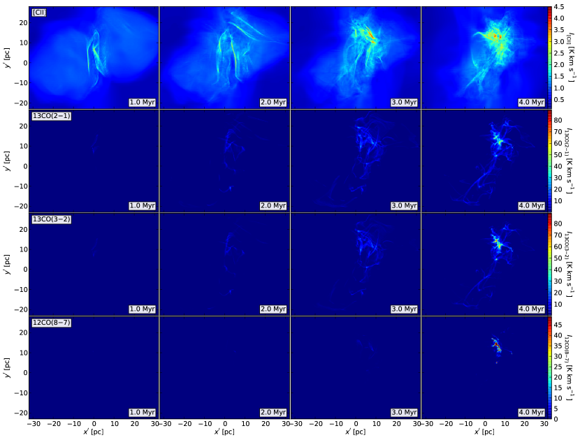
Figure 12: Time evolution of the fiducial colliding GMC model, simulating various line emissivities at 1.0, 2.0, 3.0, and 4.0 Myr. Integrated intensity maps derived from the PDR-based cooling functions: Row 1: [CII]. Row 2: ¹³CO($J$=2-1). Row 3: ¹³CO($J$=3-2). Row 4: ¹²CO($J$=8-7).

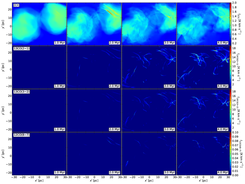
Figure 13: Same as Fig. 12 except for the non-colliding case, simulating various line emissivities at 1.0, 2.0, 3.0, and 4.0 Myr. Integrated intensity maps derived from the PDR-based cooling functions: Row 1: [CII]. Row 2: ¹³CO($J$=2-1). Row 3: ¹³CO($J$=3-2). Row 4: ¹²CO($J$=8-7).

Figures 12 and  13 show the time-evolution of maps of [CII], ¹³CO($J$=2-1), ¹³CO($J$=3-2), and ¹²CO($J$=8-7) integrated intensity for the fiducial colliding and non-colliding cases, respectively.

[CII] acts as a probe for the lower density, PDR gas enveloping GMCs. This region contains gas transitioning to the molecular phase and joining the GMC material. Our synthetic maps of [CII] show emission in extended regions surrounding the denser gas. The colliding case exhibits higher [CII] intensities, but over a smaller volume concentrated about the converging flows. The original GMCs show $I_{\rm[CII]}\sim 1\>{\rm K~{}km/s}$, with subsequent evolution reaching up to $\sim 4\>{\rm K~{}km/s}$. The non-colliding case remains at $\sim 1\>{\rm K~{}km/s}$ throughout the evolution, keeping a fairly consistent distribution. The emission is extended and encompasses the denser molecular gas.

¹³CO($J$=2-1), ¹³CO($J$=3-2) are seen to be good tracers of cold, dense gas. As both colliding and non-colliding clouds evolve, dense filaments form and become traceable by these low-$J$ CO lines. Noting the differences in integrated intensity scales between the two models, the densities in the colliding case reach significantly higher levels at earlier times compared to the non-colliding case and can be traced through CO. The morphologies of the structures differ, as one primary dense filamentary region can be seen being formed at the interface of the colliding flows, while distinct, distributed filaments are formed for the non-colliding case. The primary filamentary structure in the colliding case exhibits dense clumps reaching $I\approx 80\>{\rm K~{}km/s}$, while the separate filaments evolving in the non-colliding case reach values of $I\approx 20\>{\rm K~{}km/s}$ for both ¹³CO($J$=2-1) and ¹³CO($J$=3-2).

Stark differences, however, can be seen in ¹²CO($J$=8-7), where high intensities are produced later in the evolution of the fiducial colliding case, as the dense filaments in both GMCs collide and merge. These begin to become visible at $t\approx 3\>{\rm Myr}$ and reach levels of $\sim 10^{3}\>{\rm K~{}km/s}$. In the non-colliding case, there is almost no emission at this rotational level, indicating a lack of strong shocks. By the $t\approx 4\>{\rm Myr}$ mark, only $I_{\rm 12CO(J=8-7)}\sim 0.2\>{\rm K~{}km/s}$ can be detected.

3.5 Kinematics

Synthetic spectra were created to gain more quantitative comparisons between the various emission lines as well as to understand the kinematics of the models. Additionally, line-of-sight velocity spectra can be directly compared to those measured from observed clouds.

The majority of cloud collision candidates have relied primarily on multiple velocity components deduced from CO spectra in conjunction with coherent density structures and/or young stars as evidence for detection. The current study offers a unique method of directly reproducing various CO spectra for clouds undergoing collisions and comparing them with non-colliding scenarios.

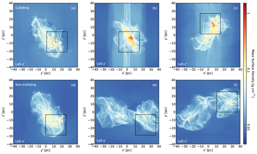
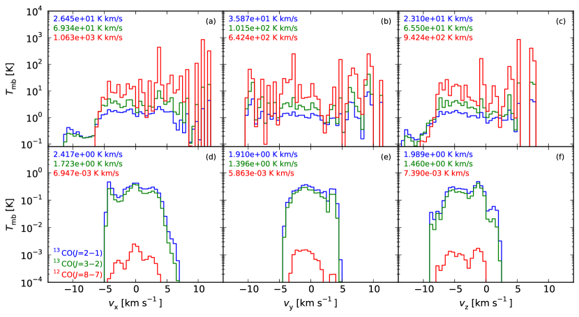
Figure 14: Top: Mass surface density maps are shown for various lines of sight directed through the fiducial colliding case (top row:(a)-(c)) and non-colliding case (bottom row:(d)-(f)). The black boxes bound equal-volume regions containing the primary filament in each simulation at $t$=4.0 Myr. Bottom: Synthetic velocity spectra for ¹³CO(2-1), ¹³CO(3-2), ¹²CO(8-7) from the respective selected regions shown in the upper figures. Note large differences in ¹²CO(8-7) integrated intensities relative to ¹³CO(2-1) and ¹³CO(3-2) between the colliding and non-colliding models.

3.5.1 Spectra

In Figure 14, we have created spectra of ¹³CO($J$=2-1), ¹³CO($J$=3-2), and ¹²CO($J$=8-7) (same as the integrated intensity maps) through square patches of area $(25.6\>{\rm pc})^{2}$ projected through the x, y, and z lines of sight for both the fiducial colliding and non-colliding cases. Each spectrum corresponds to the respective mass surface density map, on which the projected patch is indicated. The patches center on the highest mass surface density regions for both cases.

The first main difference seen in the spectra between the colliding and non-colliding cases is the width of the velocity ranges. The non-colliding case exhibits fairly narrow ($\Delta v\lesssim 10\>{\rm km/s}$) velocity widths for each line of sight. The colliding case, on the other hand, has broader ($\Delta v\sim 15-20\>{\rm km/s}$) velocity widths and what may be interpreted as multiple components, at least for the $v_{x}$ and $v_{y}$ directions, but to a lesser extent $v_{z}$ as well.

Another key result is the relative strength of the various CO lines. Throughout each of the non-colliding lines of sight, the strength of the integrated intensity follows the trend of

$$I_{\rm 13CO(2-1)}>I_{\rm 13CO(3-2)}>I_{\rm 12CO(8-7)}$$ (17)

The magnitudes are of the order $\sim 2$, $\sim 1$, and $\sim 2\times 10^{-3}$ K km/s, respectively. For the colliding case, the exact opposite trend is seen:

$$I_{\rm 13CO(2-1)}<I_{\rm 13CO(3-2)}<I_{\rm 12CO(8-7)}$$ (18)

with intensities of order $\sim 10$, $\sim 30$, and $\sim 4\times 10^{3}$ K km/s, respectively. Thus, the ¹²CO($J$=8-7)/¹³CO($J$=2-1) line intensity ratio is $\sim 10^{-3}$ for the non-colliding case and $\sim 10^{2}$ to $10^{3}$ for the colliding case.

As a result, measurement of CO spectra, especially the ¹²CO($J$=8-7)/¹³CO($J$=2-1) line intensity ratio, is another potentially strong diagnostic of cloud collisions. From our models, both the velocity range and especially the values of integrated intensities are differentiators between colliding and non-colliding GMCs and both appear to be generally independent of line of sight.

3.5.2 Velocity Gradients

We can determine velocity dispersions and gradients of dense structures within our simulations using synthetic ¹³CO($J$=1-0) line intensity maps and $p-v$ diagrams. Our goal is to use similar methods in determining these quantities as those used observationally in order to directly compare with GMCs and IRDCs in the Galaxy (see e.g., Hernandez & Tan, 2015, hereafter HT15).

We investigate the fiducial colliding and non-colliding cases transformed from our 3D spatial data to $p$-$p$-$v$-space for each of the $x$,$y$,and $z$ lines of sight (see Fig. 15). The velocity dispersion was defined using the intensity-weighted rms 1D velocity dispersion of the corresponding region. Velocity gradients were calculated along each spatial direction for coordinate axes orthogonal to the chosen line of sight (e.g., for $\frac{dv_{z}}{dx}$, the best linear fit was determined through each intensity-weighted cell in $(x,v_{z})$ space). Table 4 summarizes the velocity information for the fiducial colliding and non-colliding cases, for each line of sight.

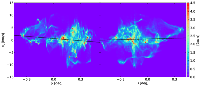
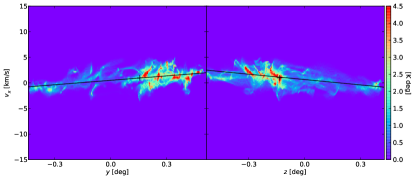
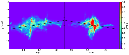
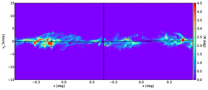
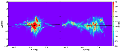
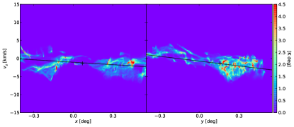
Figure 15: Position-velocity diagrams for the fiducial colliding case (left column) and non-colliding case (right column). The scaling is derived from synthetic ¹³CO($J$=1-0) line intensities through velocity bins of $\Delta v=0.212\>{\rm km\>s^{-1}}$. The black cross indicates the position of the center of mass and the solid black line shows the intensity-weighted linear velocity gradient ($dv_{\rm los}/ds$) across each cloud.

Table 4: Velocity Gradients

Case	LoS	$\sigma$ (dens)	$\frac{dv_{\rm los}}{ds}$
		($\rm{km\>s^{-1}}$)	($\rm{km\>s^{-1}\>pc^{-1}}$)
Colliding	$x$	3.6588	0.0581
	$y$	2.7611	0.1648
	$z$	2.4760	0.0278
Non-Colliding	$x$	1.4926	0.0864
	$y$	1.1996	0.0110
	$z$	1.9649	0.0948

Strong differences between the two models are revealed through the velocity dispersion, with the colliding case showing indications of much greater dispersion. The largest velocity dispersion of $\sim 3.7$ km/s is seen along the collision axis, while the orthogonal directions also experience greater dispersion relative to the non-colliding case. The RMS velocity dispersion over the 3 lines of sight is 3.01 km/s for the colliding case and 1.58 km/s for the non-colliding case.

The velocity gradients reveal differences as well. The largest velocity gradient occurs when looking in the direction of the collisional impact parameter, at $\sim 0.16$ km/s/pc. However, the gradients along the remaining directions are similar in magnitude and even somewhat smaller when compared with the non-colliding case. The RMS velocity gradient over the 3 lines of sight is 0.1022 km/s/pc for the colliding case and 0.0743 km/s/pc for the non-colliding case.

Overall, the kinematics measured in the fiducial colliding case are in rough agreement with the ten observed IRDCs and associated GMCs from HT15, in which velocity dispersions of order $\sim$few km/s and velocity gradients generally at $\sim$0.1 (but upwards of $\sim$0.6-0.7) km/s/pc were found, though these results do not necessarily preclude the non-colliding case. However, the kinematics of observed IRDCs, especially those with higher measured values of velocity gradient and dispersion, may suggest a more dynamic formation scenario with compression of GMC material.

3.6 Dynamics

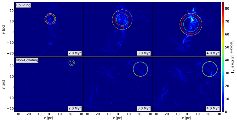
Figure 16: Time evolution maps of ¹³CO($J$=1-0) integrated intensity for the fiducial colliding case at 2.0, 3.0, and 4.0 Myr. The different effective radii calculated for the virial analysis are plotted as colored circles with radii defined by $R_{\rm M}$ (blue), $R_{\rm A}$ (green), and $R_{1/2}$ (red).

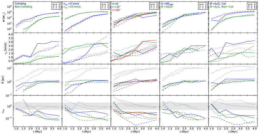
Figure 17: From top to bottom rows: Time evolution of the total mass, velocity dispersion, virial radii as defined by the areal radius $R_{\rm A}$, and the corresponding virial parameter. The columns compare the various models, as indicated by the respective color and label. The three primary lines of sight are also investigated for each model, denoted as solid ($x$), dashed ($y$), and dotted ($z$) lines. The shaded region is centered on $\alpha_{\rm vir}=1$ with a factor of 2 to each side, roughly the range seen by HT15.

Virial analysis of clouds compares the relative importance of self-gravity with internal motions and can reveal dynamical properties of the material and, in turn, provide evidence for recent kinematic history. HT15 performed virial analysis on ten observed IRDCs and associated GMCs based on ¹³CO($J$=1-0) emission and found that IRDCs have moderately enhanced velocity dispersions and virial parameters relative to GMCs, potentially indicating more disturbed kinematics of the densest gas. If GMC collisions indeed trigger the formation of IRDCs and then star clusters, virial analysis may be another important diagnostic for the products of cloud collisions.

We follow the “simple extraction (SE)” and “connected extraction (CE)” techniques detailed in HT15, applying them to our fiducial colliding and non-colliding models. First, we calculate the cloud center of mass in $p$-$p$-$v$-space based on ¹³CO($J$=1-0) intensity. SE selects all voxels with ¹³CO(1-0) emission out to radii of $R$=5,10,20, and 30 pc and within a $v_{0}\pm 15\>{\rm km\>s^{-1}}$ line-of-sight velocity range. CE, on the other hand, selects voxels directly connected face-wise in $p$-$p$-$v$-space. Each must exceed the same ¹³CO(1-0) intensity threshold of $T_{B,v}\geq 1.35$ K as in HT15, i.e., the Galactic Ring Survey (GRS) (Jackson et al., 2006) $5\sigma_{\rm rms}$ level. The connected voxel must also lie within a 30 pc radius and $\pm 15\>{\rm km\>s^{-1}}$ velocity. All connected structures in the $p$-$p$-$v$ domain are found via the established graph theory method of connected components of undirected graphs, with cells meeting the above-mentioned criteria acting as the nodes. The subgraph with the largest number of nodes is designated as the connected extraction, and further analysis is performed on this subset of voxels.

For CE, three different radii are calculated, based on various definitions: the mass-weighted radius ($R_{\rm M}$; the mean projected radial distance of cloud mass from the center of mass), areal radius ($R_{\rm A}$; from the total projected area $A=\pi R_{A}^{2}=N_{p}A_{p}$, where $N_{p}$ and $A_{p}$ are the pixel number and area, respectively, of the defined cloud), and half-mass radius ($R_{\rm 1/2}$; the radius from the center of mass that contains half the total cloud mass).

To study virialization of the cloud, we use the dimensionless virial parameter $\alpha_{\rm vir}$ from Bertoldi & McKee (1992)

$$\alpha_{\rm vir}=\frac{5\sigma^{2}R}{GM},$$ (19)

where $\sigma$ is the mass-averaged line-of-sight velocity dispersion.

Figure 16 shows the time evolution of the ¹³CO($J$=1-0) integrated intensity maps for the fiducial colliding and non-colliding cases and the corresponding virial radii. For both models, the ¹³CO($J$=1-0) structures grow in extent and encompass more material, leading to increasing effective radii. A central dominant filamentary structure forms in the colliding case, whereas the non-colliding case contains a number of smaller, more spatially separated filaments. The ¹³CO emission is generally weaker and more dispersed in independent structures in the non-colliding case. The chosen method for extraction successfully tracks the same singlelargest filamentary structure over time as it evolves in both cases.

The virial parameter and constituent variables for all models for the three $x$, $y$, and $z$ lines of sight are displayed in Fig. 17. These variables within the CE show distinctive trends over time as well as systematic differences between various models.

The total mass of the main connected ¹³CO-defined structure grows steadily over time. The fiducial colliding case produces structures that grow from $10^{3}$ to just under $10^{5}\>M_{\odot}$ over 3 Myr. The non-colliding case grows at a similar rate, but generally contains $\sim$10 times less mass. The $v_{\rm rel}=20$ km/s model creates higher-mass structures at earlier times, but converges to just over $10^{5}\>M_{\odot}$ by $t=4.0$ Myr. The $v_{\rm rel}=5$ km/s case follows an intermediate growth evolution. The $\theta=0^{\circ}$,$30^{\circ}$, and $90^{\circ}$ cases have similar mass evolution, with slightly smaller masses corresponding to increasing values of $\theta$. The total structure mass for the $b=0R_{\rm GMC}$ and $B=30~{}{\rm\mu G}$ cases grow in a similar manner. The non-magnetized colliding and non-colliding cases follow similar evolution as the fiducial colliding and non-colliding cases, respectively, but do grow to slightly larger masses in general due to the lack of magnetic pressure support.

The velocity dispersions of the ¹³CO emitting structures are found to grow throughout the time evolution for all cases, generally starting near $\lessapprox 1$ km/s and reaching 2-3 km/s. The colliding cases in general show distinctly higher velocity dispersions, especially when viewing along the collision axis ($x$). Faster collision velocities result in larger velocity dispersions, while there does not seem to be much dependence on initial magnetic field direction. Stronger magnetic fields appear to dampen the collision, resulting in slightly smaller values of $\sigma$.

The measured areal radii generally grow in a similar manner as the mass, although there is a strong dependence on viewing direction. Specifically, the $z$-directed line-of-sight, in which the plane-of-sky is sensitive to both the collision and impact parameter axes, shows a much greater radius in all cases. Along this direction, the radii are measured to increase from approximately 1 pc to 10 pc in all cases, though colliding cases in general created larger structures by a few pc. The higher velocity collisions grow much faster initially, but reach similar final spatial extents. Along the other lines of sight, there are similar trends, although the initial and final radii are approximately a factor of 10 smaller in these directions.

The general trend for all models is for the virial parameter to decrease over time, which appears to be mostly driven by the accumulation of more and more mass into the structures. The calculated radii of the structures have a strong dependence on viewing direction, as described above, thus affecting $\alpha_{\rm vir}$ as well. In the $z$ line-of-sight, where more extended structure is detected, the virial parameter values begin moderately super-virial but evolve to approach those expected of virial equilibrium, i.e., $\alpha_{\rm vir}\sim 1$ (recall $\alpha_{\rm vir}<2$ implies a gravitationally bound structure, ignoring surface pressure and magnetic pressure effects). For other viewing directions, $\alpha_{\rm vir}$ of the structure is generally smaller, often already sub-virial. Systematic differences in $\alpha_{\rm vir}$ between models are less distinct than from viewing direction, with virial parameters decreasing by factors of a few over time. Despite the small differences, the smallest values of $\alpha_{\rm vir}$ are present in the non-magnetized cases. Overall, some of these structures them may be undergoing rapid global collapse, but more likely in the magnetized cases the $B$-fields are providing support that may keep them closer to virial equilbrium. We expect that: (1) the structures will continue to accumulate mass and become even more gravitationally bound; (2) they are likely to contain highly gravitationally unstable substructures, e.g., the dense filaments and clumps that appear from 3 to 4 Myr in the fiducial colliding case.

Results from the 10 IRDCs/GMCs studied in HT15 show relatively large variation of derived virial parameter depending on the analysis method: in particular, the most relevant method for comparison with our analysis is “CE,$\tau$”, i.e., connected extraction of a structure where an optical depth correction has been assessed, and where the velocity dispersion is measured directly from the second moment of the spectrum. This method finds values of $\alpha_{\rm vir}\sim 1$, but with significant dispersion of about a factor of two. Still these values are somewhat larger than those seen in most of our simulations at $t\sim 4$ Myr. In the context of the GMC-GMC collision scenario, this may indicate that the relevant timescale for comparison is at earlier times, e.g., $t\sim 1$ to 2 Myr, or that the typical line of sight to GMCs is in a direction that includes a significant component of the collision velocity axis (which is likely for collisions mediated by shear in the Galactic disk).

While the values of $\alpha_{\rm vir}$ are similar between all of the simulations, ranging from slightly to strongly gravitationally bound objects, the total masses and velocity dispersion are notably larger for the colliding cases. Thus we conclude that, in comparison to the ¹³CO emitting structures formed in non-colliding simulations, those formed via GMC collisions are more likely to lead to the conditions necessary for massive star cluster formation.

4 Discussion and Conclusions

We have investigated physical properties associated with and potential observational signatures of magnetized, turbulent GMCs collisions. Our method has utilized PDR-based heating and cooling functions, developed in our previous study with 2D simulations, to allow our new 3D simulations, with resolution of 0.125 pc, to follow the multi-phase, non-equilibrium, thermal evolution of the clouds, including their shock structures. We have explored the parameter space of GMC collisions, including the effects of collision velocity, impact parameter, magnetic field orientation and strength. We have also carried out detailed comparisons of the results of otherwise identical colliding and non-colliding clouds.

We have found that the relative orientations between magnetic fields and mass surface density structures may be used to diagnose a cloud collision. HROs and subsequent histogram shape parameter analysis reveal distinguishing behavior resulting from cloud collisions compared with non-colliding clouds. In particular, the collision velocity appears to have a strong effect on the HRO shape parameter. The dependence on line of sight is fairly low, strengthening the $\psi$ vs. $\Sigma$ diagnostic.

The $|B|$ vs. $n_{\rm H}$ relation found in our models reveals somewhat stronger magnetic field strength when compared to the “Crutcher relation”, although the general trend appears to follow $B_{\rm max}\propto(n_{\rm H})^{2/3}$ at higher densities while staying near roughly constant $|B|$ at lower densities. This behavior is likely sensitive to our choices of initial conditions, but may be representative of regions of slightly higher mean field strength compared to the relatively nearby objects which comprise the “Crutcher relation”.

Area and mass-weighted $\Sigma$-PDFs show large differences among our models, with strong distinguishing factors between colliding and non-colliding cases. Although it is just a single case, a comparison with the $\Sigma$-PDF of an observed IRDC finds that the evolved GMC collision cases have more similar $\Sigma$-PDFs than the results of non-colliding simulations.

Intensity mapping of CO spectra, especially the ¹²CO($J$=8-7)/¹³CO($J$=2-1) line intensity ratio, is another potentially strong diagnostic of cloud collisions. From synthetic spectra of our models, the integrated intensities, as well as the velocity spread, are differentiators between colliding and non-colliding GMCs and both appear to be generally independent of line of sight orientation.

Kinematically, the velocity dispersion of the colliding case was found to be much higher than that of the non-colliding case, at almost a factor of 2 higher, reaching $\sigma>3.5\>{\rm km\>s^{-1}}$ when measured along the collision axis. Velocity gradients are also enhanced due to collisions, with the highest values in the colliding case measured when viewing orientation is along the same direction that the clouds are offset via the impact parameter, at $dv_{\rm los}/ds=0.20\>{\rm km\>s^{-1}\>pc^{-1}}$.

Finally, study of the ¹³CO-defined structures formed in the colliding and non-colliding scenarios are quite different. In all of the colliding cases, they are much more massive with generally larger velocity dispersion. Both colliding and non-colliding cases are gravitationally bound. This suggests a potential role for GMC collisions in the triggering of massive star cluster formation.

References

- Anathpindika (2009) Anathpindika, S. 2009, A&A, 504, 437
- Balfour et al. (2015) Balfour, S. K., Whitworth, A. P., Hubber, D. A., & Jaffa, S. E. 2015, MNRAS, 453, 2471
- Beck (2001) Beck, R. 2001, Space Sci. Rev., 99, 243
- Bertoldi & McKee (1992) Bertoldi, F., & McKee, C. F. 1992, ApJ, 395, 140
- Bryan et al. (2014) Bryan, G. L., Norman, M. L., O’Shea, B. W., et al. 2014, ApJS, 211, 19
- Butler et al. (2014) Butler, M. J., Tan, J. C., & Kainulainen, J. 2014, ApJ, 782, L30
- Cabral & Leedom (1993) Cabral, B., & Leedom, L. C. 1993, in Special Interest Group on GRAPHics and Interactive Techniques Proceedings, 263
- Chen et al. (2016) Chen, C.-Y., King, P. K., & Li, Z.-Y. 2016, ArXiv e-prints, arXiv:1605.00648
- Crutcher (2012) Crutcher, R. M. 2012, ARA&A, 50, 29
- Crutcher et al. (2010) Crutcher, R. M., Wandelt, B., Heiles, C., Falgarone, E., & Troland, T. H. 2010, ApJ, 725, 466
- Da Rio et al. (2014) Da Rio, N., Tan, J. C., & Jaehnig, K. 2014, ApJ, 795, 55
- Dedner et al. (2002) Dedner, A., Kemm, F., Kröner, D., et al. 2002, Journal of Computational Physics, 175, 645
- Dickel et al. (1978) Dickel, J. R., Dickel, H. R., & Wilson, W. J. 1978, ApJ, 223, 840
- Dobashi et al. (2014) Dobashi, K., Matsumoto, T., Shimoikura, T., et al. 2014, ApJ, 797, 58
- Dobbs (2008) Dobbs, C. L. 2008, MNRAS, 391, 844
- Dobbs et al. (2015) Dobbs, C. L., Pringle, J. E., & Duarte-Cabral, A. 2015, MNRAS, 446, 3608
- Federrath & Klessen (2012) Federrath, C., & Klessen, R. S. 2012, ApJ, 761, 156
- Federrath & Klessen (2013) —. 2013, ApJ, 763, 51
- Federrath et al. (2011) Federrath, C., Sur, S., Schleicher, D. R. G., Banerjee, R., & Klessen, R. S. 2011, ApJ, 731, 62
- Fiege & Pudritz (2000) Fiege, J. D., & Pudritz, R. E. 2000, ApJ, 544, 830
- Fukui et al. (2015) Fukui, Y., Harada, R., Tokuda, K., et al. 2015, ApJ, 807, L4
- Furukawa et al. (2009) Furukawa, N., Dawson, J. R., Ohama, A., et al. 2009, ApJ, 696, L115
- Gammie et al. (1991) Gammie, C. F., Ostriker, J. P., & Jog, C. J. 1991, ApJ, 378, 565
- Gutermuth et al. (2009) Gutermuth, R. A., Megeath, S. T., Myers, P. C., et al. 2009, ApJS, 184, 18
- Habe & Ohta (1992) Habe, A., & Ohta, K. 1992, PASJ, 44, 203
- Haworth et al. (2015a) Haworth, T. J., Shima, K., Tasker, E. J., et al. 2015a, MNRAS, 454, 1634
- Haworth et al. (2015b) Haworth, T. J., Tasker, E. J., Fukui, Y., et al. 2015b, MNRAS, 450, 10
- Hernandez & Tan (2015) Hernandez, A. K., & Tan, J. C. 2015, ApJ, 809, 154
- Heyer & Brunt (2004) Heyer, M. H., & Brunt, C. M. 2004, ApJ, 615, L45
- Jackson et al. (2010) Jackson, J. M., Finn, S. C., Chambers, E. T., Rathborne, J. M., & Simon, R. 2010, ApJ, 719, L185
- Jackson et al. (2006) Jackson, J. M., Rathborne, J. M., Shah, R. Y., et al. 2006, ApJS, 163, 145
- Kainulainen et al. (2009) Kainulainen, J., Beuther, H., Henning, T., & Plume, R. 2009, A&A, 508, L35
- Kainulainen & Tan (2013) Kainulainen, J., & Tan, J. C. 2013, A&A, 549, A53
- Kataoka et al. (2012) Kataoka, A., Machida, M. N., & Tomisaka, K. 2012, ApJ, 761, 40
- Kauffmann et al. (2013) Kauffmann, J., Pillai, T., & Goldsmith, P. F. 2013, ApJ, 779, 185
- Kennicutt (1998) Kennicutt, Jr., R. C. 1998, ApJ, 498, 541
- Kim et al. (2014) Kim, J.-h., Abel, T., Agertz, O., et al. 2014, ApJS, 210, 14
- Klein & Woods (1998) Klein, R. I., & Woods, D. T. 1998, ApJ, 497, 777
- Krumholz & McKee (2005) Krumholz, M. R., & McKee, C. F. 2005, ApJ, 630, 250
- Krumholz & Tan (2007) Krumholz, M. R., & Tan, J. C. 2007, ApJ, 654, 304
- Lada & Lada (2003) Lada, C. J., & Lada, E. A. 2003, ARA&A, 41, 57
- Lee et al. (2015) Lee, E. J., Chang, P., & Murray, N. 2015, ApJ, 800, 49
- Lee & Draine (1985) Lee, H. M., & Draine, B. T. 1985, ApJ, 290, 211
- Leroy et al. (2008) Leroy, A. K., Walter, F., Brinks, E., et al. 2008, AJ, 136, 2782
- Li et al. (2014) Li, H.-B., Goodman, A., Sridharan, T. K., et al. 2014, Protostars and Planets VI, 101
- Lim et al. (2016) Lim, W., Tan, J. C., Kainulainen, J., Ma, B., & Butler, M. J. 2016, ArXiv e-prints, arXiv:1605.09320
- Liszt et al. (1984) Liszt, H. S., Burton, W. B., & Xiang, D.-L. 1984, A&A, 140, 303
- Loren (1976) Loren, R. B. 1976, ApJ, 209, 466
- Loren (1977) —. 1977, ApJ, 218, 716
- McKee & Ostriker (2007) McKee, C. F., & Ostriker, E. C. 2007, ARA&A, 45, 565
- Mouschovias (2001) Mouschovias, T. 2001, in Astronomical Society of the Pacific Conference Series, Vol. 248, Magnetic Fields Across the Hertzsprung-Russell Diagram, ed. G. Mathys, S. K. Solanki, & D. T. Wickramasinghe, 515
- Murray et al. (2010) Murray, N., Quataert, E., & Thompson, T. A. 2010, ApJ, 709, 191
- Odenwald et al. (1992) Odenwald, S., Fischer, J., Lockman, F. J., & Stemwedel, S. 1992, ApJ, 397, 174
- Ohama et al. (2010) Ohama, A., Dawson, J. R., Furukawa, N., et al. 2010, ApJ, 709, 975
- Ossenkopf & Mac Low (2002) Ossenkopf, V., & Mac Low, M.-M. 2002, A&A, 390, 307
- Padoan et al. (2014) Padoan, P., Federrath, C., Chabrier, G., et al. 2014, Protostars and Planets VI, 77
- Padoan & Nordlund (2011) Padoan, P., & Nordlund, Å. 2011, ApJ, 730, 40
- Planck Collaboration et al. (2015) Planck Collaboration, Ade, P. A. R., Aghanim, N., et al. 2015, A&A, 576, A105
- Planck Collaboration et al. (2016) —. 2016, A&A, 586, A138
- Pon et al. (2015) Pon, A., Caselli, P., Johnstone, D., et al. 2015, A&A, 577, A75
- Ragan et al. (2014) Ragan, S. E., Henning, T., Tackenberg, J., et al. 2014, A&A, 568, A73
- Roman-Duval et al. (2010) Roman-Duval, J., Jackson, J. M., Heyer, M., Rathborne, J., & Simon, R. 2010, ApJ, 723, 492
- Scoville et al. (1986) Scoville, N. Z., Sanders, D. B., & Clemens, D. P. 1986, ApJ, 310, L77
- Soler et al. (2013) Soler, J. D., Hennebelle, P., Martin, P. G., et al. 2013, ApJ, 774, 128
- Solomon et al. (1987) Solomon, P. M., Rivolo, A. R., Barrett, J., & Yahil, A. 1987, ApJ, 319, 730
- Stark (1984) Stark, A. A. 1984, ApJ, 281, 624
- Suwannajak et al. (2014) Suwannajak, C., Tan, J. C., & Leroy, A. K. 2014, ApJ, 787, 68
- Takahira et al. (2014) Takahira, K., Tasker, E. J., & Habe, A. 2014, ApJ, 792, 63
- Tan (2000) Tan, J. C. 2000, ApJ, 536, 173
- Tan (2010) —. 2010, ApJ, 710, L88
- Tan et al. (2013) Tan, J. C., Shaske, S. N., & Van Loo, S. 2013, in IAU Symposium, Vol. 292, IAU Symposium, ed. T. Wong & J. Ott, 19–28
- Tasker & Tan (2009) Tasker, E. J., & Tan, J. C. 2009, ApJ, 700, 358
- Torii et al. (2011) Torii, K., Enokiya, R., Sano, H., et al. 2011, ApJ, 738, 46
- Truelove et al. (1997) Truelove, J. K., Klein, R. I., McKee, C. F., et al. 1997, ApJ, 489, L179
- Turk et al. (2011) Turk, M. J., Smith, B. D., Oishi, J. S., et al. 2011, ApJS, 192, 9
- Wang & Abel (2008) Wang, P., & Abel, T. 2008, ApJ, 672, 752
- Wu et al. (2015) Wu, B., Van Loo, S., Tan, J. C., & Bruderer, S. 2015, ApJ, 811, 56
- Zuckerman & Evans (1974) Zuckerman, B., & Evans, II, N. J. 1974, ApJ, 192, L149