NH₃(3,3) and CH₃OH near Supernova Remnants: GBT and VLA Observations

Abstract

We report on Green Bank Telescope 23.87 GHz NH₃(3,3)  emission observations in five supernova remnants interacting with molecular clouds (G1.4$-$0.1, IC443, W44, W51C, and G5.7$-$0.0). The observations show a clumpy gas density distribution, and in most cases the narrow line widths of $\sim 3-4$ km s^-1 are suggestive of maser emission. Very Large Array observations reveal 36 GHz and/or 44 GHz CH₃OH  maser emission in a majority (72%) of the NH₃  peak positions towards three of these SNRs. This good positional correlation is in agreement with the high densities required for the excitation of each line. Through these observations we have shown that CH₃OH  and NH₃  maser emission can be used as indicators of high density clumps of gas shocked by supernova remnants, and provide density estimates thereof. Modeling of the optical depth of the NH₃(3,3) emission is compared to that of CH₃OH, constraining the densities of the clumps to a typical density of the order of $10^{5}$ cm^-3 for cospatial masers. Regions of gas with this density are found to exist in the post-shocked gas quite close to the SNR shock front, and may be associated with sites where cosmic rays produce gamma-ray emission via neutral pion decay.

1. Introduction

Interactions between supernova remnants (SNRs) and molecular clouds (MCs) can cause perturbations in the gas that may affect the evolution of the surrounding interstellar medium. For example, it has long been suggested that star formation might be triggered in the parent cloud. Details of such a proposed triggering processes have not been clearly outlined and confirmed, partly due to the complexity of the regions in the inner Galaxy where the SNR/MC interactions are more probable. Another plausible effect of SNR/MC collisions is the acceleration of Galactic cosmic rays, since shock induced particle acceleration can generate relativistic energies. Models of cosmic ray acceleration usually relate the brightness of resulting $\gamma$-ray emission due to neutral pion decay using the gas number density (e.g., Drury et al., 1994; Abdo et al., 2010; Cristofari et al., 2013). The density estimates deduced from $\gamma$-ray emission measurements are often larger (10-20 times) than those inferred from X-ray observations, indicating a strongly clumped medium is required to produce the $\gamma$-ray emission (e.g., Slane et al., 2015). Detailed density estimates, and density gradients, in regions associated with $\gamma$-ray emission are thus of interest to constrain the inputs of cosmic ray acceleration models. Observations of molecular transitions of various molecules excited by the passing shock provides a tool to derive densities, and can also provide kinematic information of the gas. An overall understanding of the conditions in the interacting cloud, both pre- and post-shock, may provide basic facts to guide models of both SNR induced star formation as well as cosmic ray acceleration.

] Source Other Name RA DEC SNR Size V_LSR Distance GBT Channel noise (J2000) (J2000) (RA′$\times$DEC′) (km s^-1) (kpc) (mJy bm^-1) G049.2$-$0.7 W51C 19 23 50 +14 06 00 30$\times$20 70.0 6.0 17 G005.7$-$0.0* 17 59 02 $-$24 04 00 8$\times$8 13.0 3.2 16 G034.7$-$0.4 W44 18 56 00 +01 22 00 25$\times$30 45.0 2.5 16 G189.1+3.0 IC443 06 17 00 +22 34 00 45$\times$45 5.0 1.5 12 G001.4$-$0.1 17 49 39 $-$27 46 00 10$\times$10 $-$2.0 8.5 18

Table 1Observed SNRs

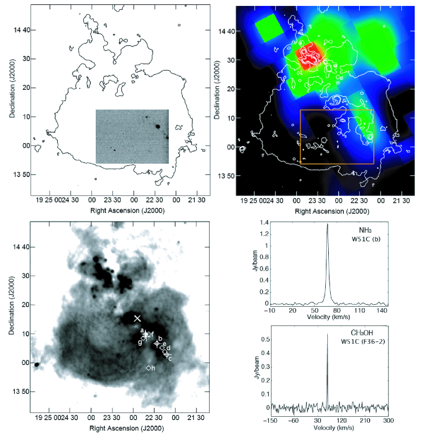
Figure 1.— Top left: NH₃ emission distribution (greyscale) outline by 90 cm radio continuum (contours at $30$ mJy beam^-1) of the W51 complex. Top right: $60-80$ km s^-1 CO(1$-$0) emission (Dame et al., 2001), indicating the interacting MC, with respect to the radio continuum (levels at 30, 150, 300, and 400 mJy beam^-1). Bottom left: 36 GHz CH₃OH masers (white plus signs) detected with the VLA with respect to NH₃ emission peaks (white diamonds), 1720 MHz OH masers (white crosses), and continuum emission (greyscale). Bottom right: Example spectral profiles of the brightest NH₃ emission region (b) and the brightest 36 GHz CH₃OH maser detected (F36-2).

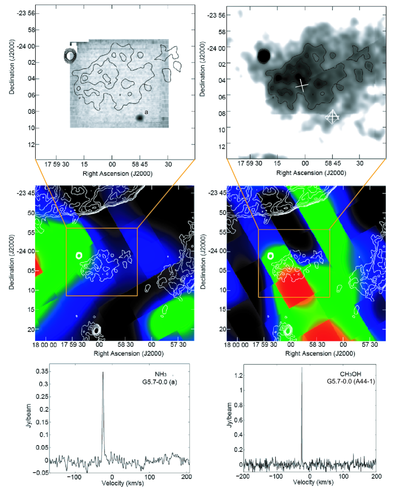
Figure 2.— Top left: NH₃ emission distribution (greyscale) overlaid on a 90 cm radio continuum (contours at 25, 37.5, 50, 75, 100, and 125 mJy beam^-1) of G5.7$-$0.0. Top right: 36 GHz (white plus sings) and 44 GHz (white triangles) CH₃OH masers detected with the VLA with respect to NH₃ emission peaks (white diamonds), 1720 MHz OH masers (white crosses), and continuum emission (greyscale). Middle left: $3-23$ km s^-1 CO(1$-$0) emission (Dame et al., 2001), which indicates the location of an interacting MC around the velocity of the OH maser ($\sim 13$ km s^-1), with respect to the radio continuum (contours). Middle right: $-16$ to $-36$ km s^-1 CO emission, which indicates the locations of another interacting MC around the velocities of the NH₃ and CH₃OH ($\sim-26$ km s^-1), with respect to the radio continuum (contours). Bottom left: Example spectral profiles of the NH₃ emission region (a). Bottom right: Example spectral profiles of the brightest 44 GHz CH₃OH maser detected (A44-1).

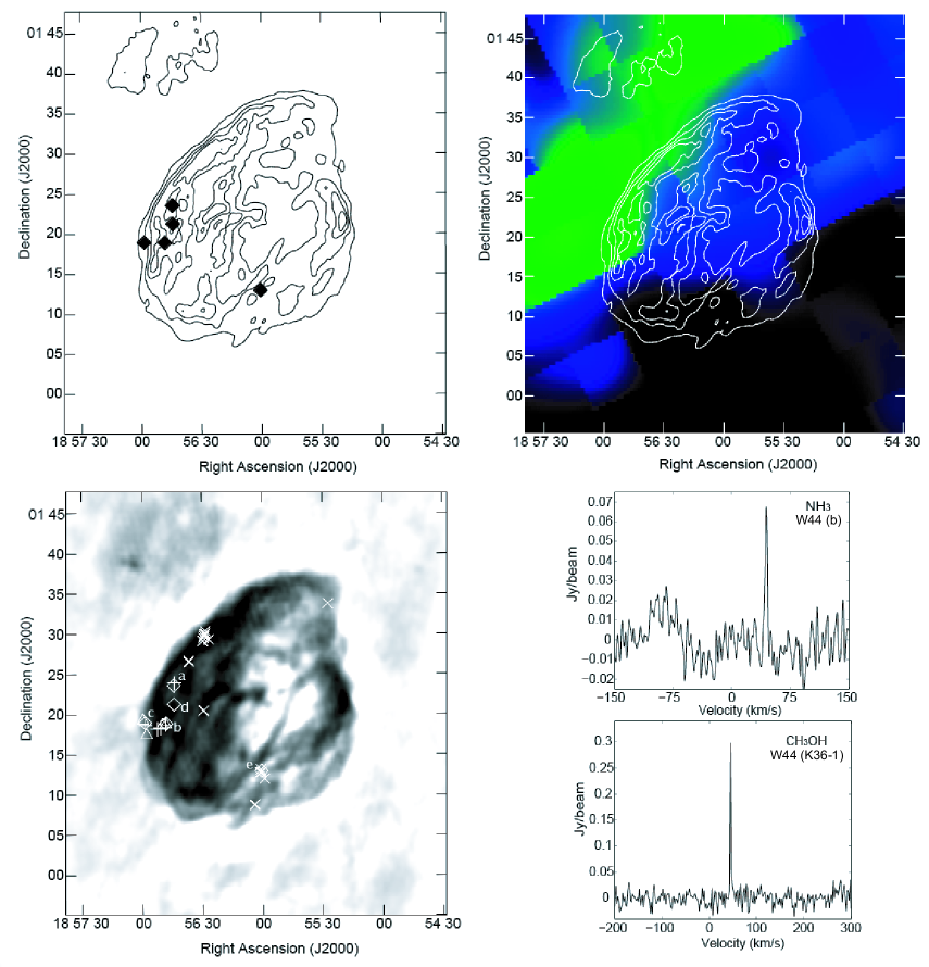
Figure 3.— Top left: NH₃ emission peaks (black diamonds) overlaid on 21 cm radio continuum (contours at 5, 25, 50, 100 and mJy beam^-1) of W44. Top right: $35-55$ km s^-1 CO emission (Dame et al., 2001), which indicates the location of the interacting MC, with respect to the radio continuum (contours). Bottom left: 36 GHz (white plus signs) and 44 GHz (white triangles) CH₃OH emission with respect to the NH₃ emission peaks (white diamonds), 1720 MHz OH masers (white crosses), and continuum emission (greyscale). Bottom right: Example spectral profiles of the brightest NH₃ emission region (b) and the brightest 36 GHz CH₃OH maser detected (K36-1).

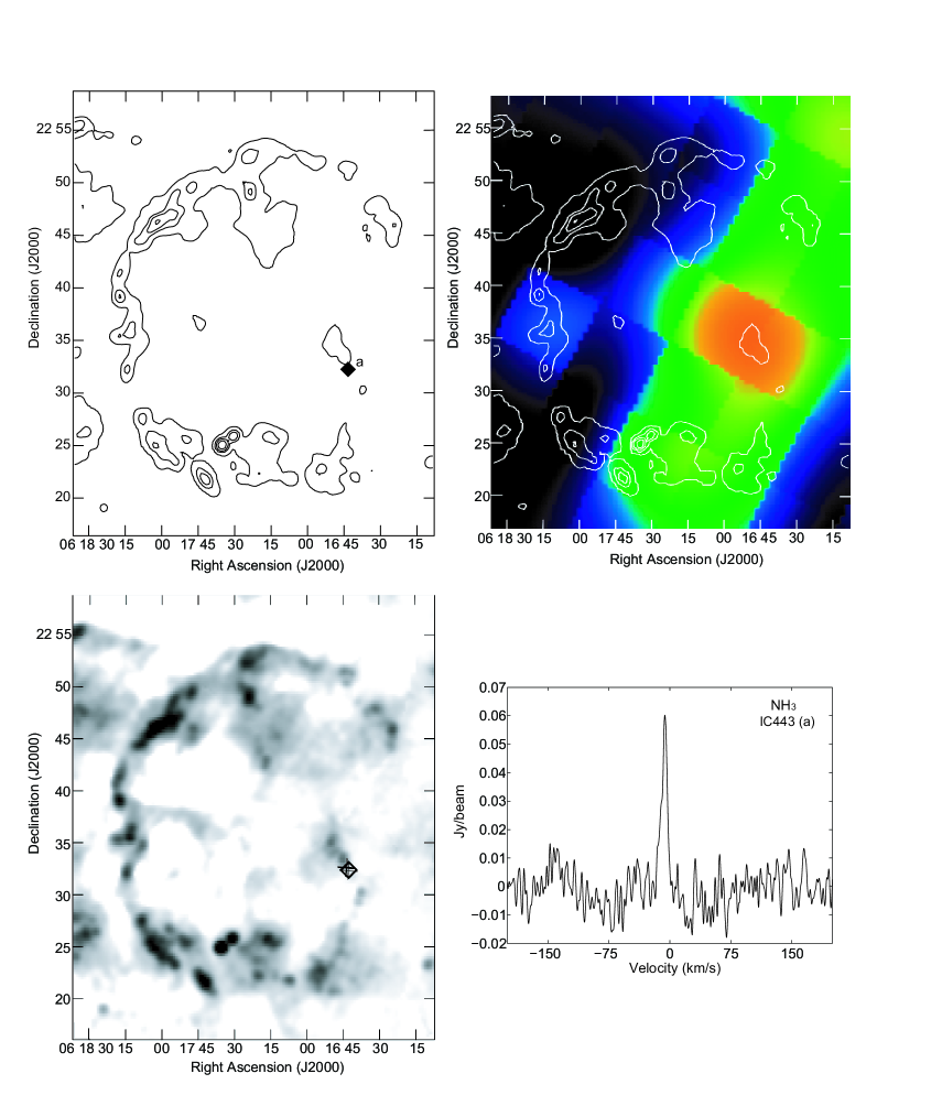
Figure 4.— Top left: NH₃ emission peak (black diamond) overlaid on 21 cm radio continuum (contours at 20, 80,140, and 200 mJy beam^-1) of IC443. Bottom left: NH₃ emission peak (black diamond) and 1720 MHz OH masers (black plus signs) with respect to the continuum emission (greyscale). Top right: $-5$ to 15 km s^-1 CO emission (Dame et al., 2001), which indicates the location of the interacting MC, with respect to the radio continuum (contours). Bottom right: Example spectral profile of the NH₃ emission region (a).

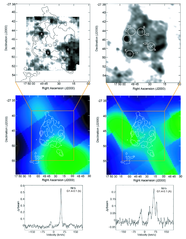
Figure 5.— Top left: NH₃ emission distribution (greyscale) outline by 21 cm radio continuum (contours at 4.3, 8.6, 17.2, and 34.4 mJy beam^-1) of G1.4$-$0.1. The bright NH₃ regions (labeled a through d) have spectral features listed in Table 2. Top right: Average positions of the 36 GHz CH₃OH masers (white plus sings) in each pointing (white circles labeled with the letters A through E and the average velocity in km s^-1) detected by Pihlström et al. (2014) with respect to 1720 MHz OH masers (white crosses), and continuum emission (greyscale). Middle left: $20-30$ km s^-1 CO emission (Dame et al., 2001), which indicates the location of an interacting MC, with respect to the radio continuum (contours). Middle right: $-15$ to $-30$ km s^-1 CO emission, which indicates the locations of another interacting MC, with respect to the radio continuum (contours). Bottom row: Example spectral profiles of the NH₃ emission in region b (left) and region A (right).

SNR/MC interactions are identified in different ways, for example, via shock excited OH 1720 MHz emission (Claussen et al., 1997; Wardle, 2002), near-infrared H₂ emission, and broad molecular line widths exceeding those of cold molecular gas (Reach et al., 2005). In addition to the 1720 MHz OH, other shock excited masers detected in SNR/MC regions include the Class I 36 GHz and 44 GHz methanol (CH₃OH) masers, which can be used to estimate densities in the maser emitting region (Sjouwerman et al., 2010; Pihlström et al., 2011, 2014; McEwen et al., 2014). In characterizing physical parameters of gas clouds in general, the ammonia (NH₃) molecule is commonly used as a probe of dense ($n\geq 10^{3}$ cm^-3) environments. Ratios of the line intensities allow estimates of rotational excitation temperatures, heating, and column densities (e.g., Morris et al., 1983; Ho & Townes, 1983; Okumura et al., 1989; Coil & Ho, 1999). Illustrating examples of where NH₃ information can be combined with that of maser species include the high resolution observations of NH₃ in the inner 15 pc of the Galactic center (GC) region (Coil & Ho, 1999, 2000; McGary et al., 2001), and the recent detections of Class I 36 GHz and 44 GHz CH₃OH maser emission toward Sgr A East (Sjouwerman et al., 2010; Pihlström et al., 2011; McEwen et al., 2016). These observations reveal a close positional agreement between the NH₃ emission peaks and the location of CH₃OH masers. A similar spatial coincidence between NH₃ and 44 GHz CH₃OH masers has also been found toward W28 (Sjouwerman et al., 2010; Nicholas et al., 2011; Pihlström et al., 2014).

A relatively general picture of the distribution of OH and CH₃OH  masers in SNRs comes from observations of Sgr A East, W28, and G1.4$-$0.1 (e.g., Sjouwerman et al., 2010; Pihlström et al., 2011, 2014; McEwen et al., 2014). Based on these observations, it has been shown that CH₃OH masers are typically found offset from 1720 MHz OH masers (e.g., Claussen et al., 1997; Frail & Mitchell, 1998; Yusef-Zadeh et al., 2003; Sjouwerman et al., 2010; Pihlström et al., 2014). This indicates that particular maser species and transitions are tracing different shocked regions, or alternatively, different regions in one shock. Consistently, bright 36 GHz CH₃OH masers have been found to trace regions closer to the alleged shock front and OH masers are more likely to trace the post-shocked gas. The location of the 44 GHz masers relative to the shock front has been less clear.

To further develop the general picture of the pre- and post-shock gas structures in SNR/MCs, including the presence and spatial positions of different molecular transitions through the interaction region, the NRAO Green Bank Telescope (GBT) was used to survey five SNRs (W51C, W44, IC443, G1.4$-$0.1, and G5.7$-$0.0) for NH₃ emission (Sect. 2.1). Here we report on the spatial distribution of the NH₃(3,3) emission compared to that of the 36 and 44 GHz CH₃OH maser emission previously observed by Pihlström et al. (2014) in G1.4$-$0.1 and the emission detected in new observations in W51C, W44, and G5.7$-$0.1 using the Very Large Array, VLA (Sect. 2.2). Section 3 discusses the results from the observations. Estimates of the temperature and density ranges most suitable for the formation of NH₃(3,3) masers in an SNR environment are provided using model calculations (Sect. 4), and compared to those of the CH₃OH masers (Sect. 5).

2. Observations and Data Reduction

2.1. GBT Observations and Data Reduction

Observations were carried out using the GBT in January through May of 2013 under the project code GSLT051174. An original list of 17 possible targets was considered based on previously known SNR/MC interaction sites (detected via 1720 MHz OH masers). The allocated time allowed four targets to be fully mapped (G5.7$-$0.0, IC443, W44, and G1.4$-$0.1) and one target to be partially mapped (W51C). Characteristics of each SNR observed, such as size and systemic velocity, can be found in Table 1. It should be noted that the source G5.7$-$0.0 has not yet been confidently classified as an SNR because it is very faint in the radio, and does not have a typical shell-like morphology (Brogan et al., 2006). It is considered a SNR candidate since it displays non-thermal emission and is associated with an 1720 MHz OH maser, indicative of a MC/SNR shocked interaction (Hewitt & Yusef-Zadeh, 2009). The sources were surveyed for NH₃ emission using the 7-beam K-band focal plane array (KFPA) and spectrometer. The observations were made with dual polarization, 50 MHz of bandwidth having a total velocity coverage of about 600 km s^-1 and a velocity resolution of about 0.5 km s^-1. Venus, Jupiter, Saturn, and the Moon were used as calibrators depending on which source was visible at the time of each observation. The DECLAT and RALONG standard spectral line survey mapping modes were used, with a slew rate of around 3.6″ s^-1. In-band and out-of-band frequency switching were utilized depending on the proximity of the SNR to the GC, assuming possible velocities $\pm 200$ km s^-1, or more for $|\ell|<25^{\circ}$.

The data reduction and calibration was carried out using the GBT pipeline following standard procedures outlined in the GBTPIPELINE User’s Guide. The GBT pipeline procedure was used to automate the calibration and combine the data from multiple observing sessions. The pipeline estimates the atmospheric opacity by using real-time weather monitored data. Astronomical calibrator sources were used to correct the system temperatures of the beams by applying gain factors (one for each beam and polarization) that were acquired using venuscal, jupitercal, saturncal, and mooncal procedures in GBTIDL. In a few instances the reported system temperatures where corrupted, in which case average gain factors were calculated from all observing sessions combined. This caused a slightly larger error of the absolute flux density value measured, but this does not affect the results reported on in this paper. Finally, the beginning and ending channels were clipped during the pipeline procedure, which varied for each data set.

Channel averaging, continuum subtraction, and imaging were carried out in AIPS using standard data reduction and imaging tasks applied to single dish data. Every two channels were averaged and all the data were Hanning-smoothed. A third-order polynomial fit was subtracted from the line free channels over the entire bandwidth. An additional third-order polynomial fit was subtracted (outside AIPS) from the NH₃ emission in W44 and IC443 to make the baselines more linear, which we suspect were affected by severe weather conditions at the time of the observations. Some of the SNRs are very large and the full mapping could not be completed during one observing session, therefore, the mapped regions were produced by combining different data sets from different observing sessions. As a result, the root mean square (RMS) noise level varies across these maps, which can primarily be attributed to the varying weather conditions on the different days of observation. The average RMS noise values in a line free channel for each target using the GBT are listed in column 8 of Table 1.

Table 2NH₃ Emission Information

& NH₃ pos RA DEC V_p $\Delta$V I_p CH₃OH Maser VLA Comment (J2000) (J2000) (km s^-1) (km s^-1) (Jy bm^-1) Association (GHz) Data W51Ca 19 22 42.15 $+$14 09 54.0 60.7 4.1 0.12 36 Y W51Cb 19 22 26.07 $+$14 06 42.0 67.5 3.4 1.39 36 & 44 Y Fig. 1 W51Cc 19 22 12.07 $+$14 02 48.0 68.7 3.4 0.19 36 & 44 Y W51Cd 19 22 15.36 $+$14 03 48.0 71.2 4.3 0.10 44 Y W51Ce 19 22 19.07 $+$14 05 12.0 70.8 4.0 0.07 44 Y W51Cf 19 22 37.62 $+$14 09 54.0 66.9 3.1 0.06 ^∗∗ Y W51Cg 19 22 46.28 $+$14 08 18.0 66.9 3.1 0.06 ^∗∗ Y W51Ch 19 22 38.05 $+$13 58 12.0 61.0 4.0 0.06 ^∗∗ Y G5.7-0.0a 17 58 45.05 $-$24 08 48.0 $-$25.1 3.7 0.37 36 & 44 Y Fig. 2 W44a 18 56 44.21 $+$01 23 34.7 40.9 4.4 0.06 36 Y W44b 18 56 48.21 $+$01 18 52.7 44.6 5.5 0.07 36 & 44 Y Fig. 3 W44c 18 56 58.62 $+$01 18 46.7 46.5 4.0 0.05 36 & 44 Y W44d 18 56 46.21 $+$01 21 16.7 41.9 3.4 0.05 ^∗∗ Y W44e 18 56 01.80 $+$01 12 40.7 44.0 3.6 0.06 ^∗ Y IC443a 17 16 42.97 $+$22 32 23.9 $-$6.1 6.7 0.06 ^∗ Y Fig. 4 G1.4-0.1a 17 49 48.14 $-$27 44 42.0 $-$31.7 11.7 0.16 36 Y 47.4 3.7 0.48 36 G1.4$-$0.1b 17 49 41.36 $-$27 48 60.0 $-$20.6 8.3 0.07 ^∗∗∗ N Fig. 5 50.5 7.4 0.58 ^∗∗∗ G1.4$-$0.1c 17 49 20.10 $-$27 48 24.0 $-$37.5 16.0 0.17 ^∗∗∗ N 69.8 15.3 0.48 ^∗∗∗ G1.4$-$0.1d 17 49 24.62 $-$27 50 18.0 $-$9.7 12.6 0.09 ^∗∗∗ N 25.4 10.4 0.40 ^∗∗∗ 87.9 13.2 0.25 ^∗∗∗ G1.4$-$0.1A 17 49 31.09 $-$27 47 36.3 $-$23.4 11.7 0.10 36 Y Fig. 5 34.6 13.3 0.11 36 64.3 13.2 0.24 36 82.7 8.9 0.15 36 G1.4$-$0.1B 17 49 37.59 $-$27 44 20.4 $-$31.7 13.2 0.61 36 Y G1.4$-$0.1C 17 49 46.79 $-$27 44 08.8 $-$31.0 15.9 0.12 36 Y 44.7 10.4 0.27 36 G1.4$-$0.1E 17 49 49.97 $-$27 49 14.9 $-$18.5 14.1 0.12 36 Y ${}^{*}\phantom{{}^{**}}$ Searched in a previous study by Pihlström et al. (2014) but no CH₃OH was detected. ${}^{**}\phantom{{}^{*}}$ Searched in this study but no CH₃OH was detected. ^∗∗∗ This area has not been searched to date.

2.2. VLA Observations and Calibration

The VLA was used to search for CH₃OH emission towards the NH₃ peak positions found with the GBT (excluding positions previously searched). Note that one of the primary reasons for the GBT observations was to obtain positions of NH₃ peaks. Even though some of the detected NH₃ emission was very weak, e.g., in W44, they were still included in the VLA search. The data were acquired on September 4, 2014 (project code 14A-191) using the Ka$-$band and Q$-$band receivers. To cover the spatial extent of the NH₃ emission, 1(1), 11(17) and 12(14) pointings at 36(44) GHz were used in G5.7$-$0.0, W44 and W51C, respectively. The array was in D configuration resulting in typical synthesized beam sizes of 2.65″$\times$1.90″ at 36 GHz and 2.11″$\times$1.84″ at 44 GHz. The VLA primary beam is 1.25′ at 36 GHz and 1.02′ at 44 GHz.

512 frequency channels were used across a 128 MHz bandwidth (channel separation close to 1.9 km s^-1), centered on the sky frequency of the given target estimated using the previously known OH maser emission. The data were calibrated and imaged using standard procedures in AIPS pertaining to spectral line data. For each pointing position, the on-source integration time was approximately 1(2) minutes at 36(44) GHz. The precise integration time varied somewhat between the positions depending on how the observations fit within the scheduling block. The typical final RMS noise values were between about 12 and 40 mJy per channel, depending on the observed frequency and observing conditions. Under ideal weather conditions, the theoretical RMS noise would be close to 10 mJy beam^-1. Degraded weather and a varying number of antennas in the array is consistent with the slightly higher measured RMS noise. No 36 GHz or 44 GHz continuum emission was found in any of the observed fields.

Table 3CH₃OH Maser Emission Information

Source	$\nu$	Name	RA	DEC	Vp	$\Delta$V	Ip
	(GHz)		(J2000)	(J2000)	(km s-1)	(km s-1)	(Jy bm-1)
W51C	36	B36-1	19 22 42.69	$+$14 09 55.5	57.6	6.0	0.25
	36	B36-2	19 22 42.21	$+$14 09 51.5	59.6	4.7	0.14
	36	B36-3	19 22 42.76	$+$14 10 02.0	57.6	3.0	0.13
	36	B36-4	19 22 41.42	$+$14 09 03.5	74.1	10.0	0.24
	36	F36-1	19 22 25.70	$+$14 06 35.0	65.9	3.1	0.43
	36	F36-2	19 22 26.01	$+$14 06 36.0	65.9	2.5	0.54
	36	F36-3	19 22 26.11	$+$14 06 37.0	63.8	4.0	0.50
	36	L36-1	19 22 12.08	$+$14 02 49.5	67.9	4.0	0.43
	36	L36-2	19 22 07.34	$+$14 02 18.5	76.2	4.0	0.19
G5.7$-$0.0	36	A36-1	17 58 44.99	$-$24 08 38.0	$-$26.4	3.5	0.38
	36	A36-2	17 58 45.17	$-$24 08 39.5	$-$26.4	4.0	0.26
	36	A36-3	17 58 44.85	$-$24 08 36.5	$-$26.4	4.0	0.21
	44	A44-1	17 58 44.48	$-$24 08 37.0	$-$24.4	1.8	1.31
	44	A44-2	17 58 44.88	$-$24 08 37.0	$-$24.4	3.0	0.35
W44	36	A36-1	18 56 43.96	$+$01 23 54.2	40.9	3.0	0.25
	36	F36-1	18 56 48.39	$+$01 18 45.7	42.9	2.0	0.09
	36	G36-1	18 56 50.82	$+$01 18 17.3	42.9	4.5	0.14
	36	G36-2	18 56 50.86	$+$01 18 21.8	40.9	4.5	0.11
	36	G36-3	18 56 52.49	$+$01 18 12.3	47.1	7.0	0.12
	36	K36-1	18 56 58.46	$+$01 18 41.7	45.0	2.7	0.30
	44	K44-1	18 56 49.86	$+$01 18 43.2	56.9	0.7	0.21
	44	L44-1	18 56 48.36	$+$01 18 46.2	45.0	1.6	0.31
	44	P44-1	18 56 57.86	$+$01 17 27.7	35.6	1.1	0.26
	44	Q44-1	18 56 59.69	$+$01 19 17.2	6.7	1.5	0.24

2.3. Radio Continuum and CO Line Images

To visualize the spatial distribution emission across each SNR, low-frequency radio continuum maps were assembled from archival data. The 21 cm IC443 map was taken from the NRAO VLA Sky Survey (NVSS; Condon et al. 1998). The 21 cm images of W44 and G1.4$-$0.1 were made from VLA archive data taken in 1984 and 1995, respectively, using standard AIPS calibration and imaging procedures. The 90cm W51C and G5.7$-$0.0 images were obtained and adapted from Brogan et al. (2013) and Brogan et al. (2006), respectively. A comparison of the NH₃ and CH₃OH distribution with CO(1$-$0) is also presented, using images from the Dame et al. (2001) Milky Way CO survey.

3. Results

3.1. NH₃ Emission

NH₃(3,3) emission was detected towards all the SNRs observed. Four of the targets (G5.7$-$0.0, W44, W51C, and IC443) display compact clumps of emission, with the majority having relatively narrow line widths of $\sim 3-4$ km s^-1, see Figs. 1-4. G1.4$-$0.1 has a much more extended distribution of the emission, and has peaks combined into broader lines with widths closer to $8-16$ km s^-1 (Fig. 5). The peak position, velocity centroid, velocity width, and the peak flux density of each emission region is listed in Table 2. For each SNR, the brightest spectral profiles are plotted in Figs. 1-5. Included in Figs. 1-5 are the spatial positions of the NH₃ emission regions overlaid on radio continuum maps outlining details and boundaries of each SNR (in greyscale and contours). In addition, the radio continuum is overlaid on CO(1$-$0) maps averaged over the velocities corresponding to those of the NH₃ emission. This shows the interacting MCs with respect to each SNR.

The narrow linewidths may indicate maser emission from the metastable NH₃(3,3) transition. In the case of G1.4$-$0.1, the extended emission combined with broader linewidths may be the result of maser emission mixed with thermal emission. The angular resolution of the GBT is not sufficient to set strong limits of the brightness temperature, which could have provided further information on the possibility of maser emission. With no data from the lower metastable states (the (1,1) and (2,2) transitions) and with limited resolution, further studies to investigate the candidate maser will have to be performed.

3.2. CH₃OH  Maser Candidates

CH₃OH maser emission was detected in two SNRs (W44 and W51C) and in the one candidate SNR (G5.7$-$0.0) observed. Typical FWHMs range from about 0.7 to 10 km s^-1. Features labeled as detections all had a signal-to-noise ratio greater than 5 in the centroid channel, and emission was detected in three or more channels. The positions, centroid velocities, FWHMs, and peak flux densities of the candidate maser features found in our new VLA observations are listed in Table 3. The FWHMs are narrow, and example spectral profiles of the brightest maser associated with each SNR can be found in Fig. 1 to 3. Note that due to the combination of a small VLA field-of-view and the limited observing time, the CH₃OH emission search did not cover the entire SNR/MC interaction regions.

The emission regions were unresolved with the VLA, except for the 36 GHz emission in G5.7$-$0.0. The emission in this source was marginally resolved and had three peak flux density positions. CH₃OH maser candidates were detected in the majority of the pointings. Although 44 GHz maser candidates were visible towards W51C, we chose not to include those in Table 3, due to a significantly increased noise in this data set caused by a standing wave feature of unknown origin.

3.3. CH₃OH and NH₃ Association

Table 2 lists the NH₃ regions that have positional association with 36 and/or 44 GHz CH₃OH candidate masers. The brightest NH₃ regions associated with W44, W51C, and G5.7$-$0.0 have both 36 and 44 GHz CH₃OH candidate maser association. Overall, 14 out of 20 (72%) positions observed in both the NH₃(3,3) and CH₃OH display emission from both molecular species.

4. Optical Depth Modeling

The relative intensity of co-located molecular emission transitions can be used to estimate the physical condition of the gas. In McEwen et al. (2014), the MOLPOP-CEP code for coupled radiative transfer and level population calculations was used to estimate the conditions conducive for 36 GHz and 44 GHz CH₃OH masers in SNRs. To compare the range of temperature and densitites producing NH₃(3,3) maser emission with that of the CH₃OH maser, the same code was used to determine the optical depth of the NH₃(3,3) transition. Following the same assumptions of the SNR conditions as in McEwen et al. (2014), an external radiation field of 2.725 K from the CMB and a 30 K dust radiation field were used in the models. Energy levels for the NH₃(3,3) molecule were incorporated using the Leiden Atomic and Molecular Database (LAMDA), which includes 22 and 24 energy levels for the ortho- and para-species, up to 554 and 294 cm^-1, respectively (Schöier et al., 2005). The collision rate coefficients were also adopted from LAMDA, including temperatures ranging from 15 to 300 K. The optical depth was calculated for the NH₃(3,3) line for a density range of 10${}^{2}-10^{8}$ cm^-3, a temperature range of 20–300 K, and a fractional abundance of NH₃ of 10^-7. The results are plotted in Fig. 6, showing a well defined peak of the optical depth around a density of 10⁵ cm^-3 with an increasing peak value for warmer temperatures.

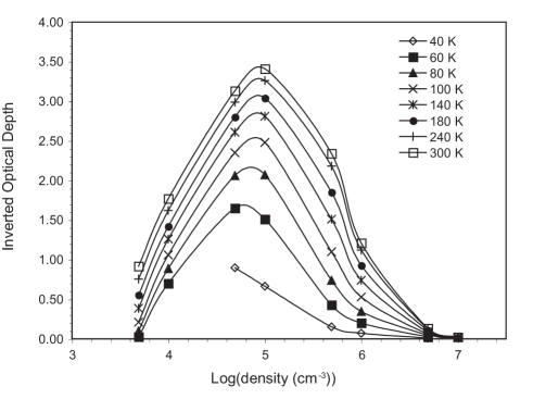
Figure 6.— Peak inverted optical depth versus number density of H₂, with a clear peak for densities around 10⁵ cm^-3.

5. Discussion

The fact that CH₃OH and NH₃(3,3) trace the same clumps of gas allow estimates of the density and temperature in localized regions. If the regions are within the positional error bars of $\gamma$-ray emission, these estimates may provide interesting information of the conditions of gas that may be linked with cosmic ray acceleration. Here we discuss the density and positions of the shocked regions with respect to the SNRs.

5.1. Density and Temperature

McEwen et al. (2014) estimated the conditions conducive for CH₃OH 36 GHz and 44 GHz masers in SNRs. Their results show a comparably brighter 36 GHz maser in higher density regimes ($n>10^{5}$ cm^-3), and a more dominant 44 GHz maser at lower densities ($n<10^{5}$ cm^-3) for an optimal temperature $T<150$ K. The (3,3) inversion transition of NH₃ has a temperature of about 100 K above ground, and therefore the emission distribution will emphasize excited gas. NH₃(3,3) maser emission can occur via collisions with H₂ molecules (Walmsley & Ungerechts, 1983; Mangum & Wootten, 1994; Zhang & Ho, 1995). Through statistical calculations it was found that NH₃(3,3) masers occur in gas with temperatures around 200 K and densities on the order of $10^{3.5}-10^{7}$ cm^-3 (e.g. Mauersberger et al., 1986; Mangum & Wootten, 1994). Consistent with previous calculations, the MOLPOP-CEP estimates performed for our SNR environment (Sect. 4) show optimal NH₃ maser conditions at relatively high temperatures ($T>150$ K) and a relatively narrow density peak around $n\approx 10^{5}$ cm^-3 . At those densities, there is, in fact, little difference in the inverted optical depth between the 36 GHz and 44 GHz masers (McEwen et al., 2014), perhaps explaining the range of line ratios observed in the SNRs (Table 3), where in some locations the 36 GHz maser is brighter, and the 44 GHz maser in others. That the line ratios of the 36 GHz and 44 GHz CH₃OH are on average unity further agrees with a relatively high temperature in the clumps. It thus seems that the co-located clumps of NH₃(3,3) and CH₃OH masers trace gas regions with $T>150$ K and $n\approx 10^{5}$ cm^-3.

G1.4$-0.1$ is the exception, where both 36 GHz CH₃OH and NH₃ emission is profuse and 44 GHz is lacking. Here, the linewidths of the NH₃ are greater and the emission may be at least partly thermal. In this case, the 36 GHz methanol might be tracing the densest clumps in the interaction regions. A better understanding of the NH₃ thermal versus non-thermal emission here could be attained by also obtaining observations of the NH₃(1,1) and (2,2) emission that may be thermal, providing even stronger limits on the temperature and density. Interferometric observations would also be helpful to tie down the brightness temperature of the NH₃(3,3) lines.

5.2. Spatial Trends

The general picture of the spatial distribution of collisionally pumped masers in SNRs was outlined in Sect. 1, where regions close to the shock front harbor 36 GHz CH₃OH masers, and post-shock regions harbor 1720 MHz OH masers. This depiction was based largely on observations of Sgr A East, W28, and G1.4$-$0.1 (e.g., Sjouwerman et al., 2010; Nicholas et al., 2011; Pihlström et al., 2011, 2014). With our new data, this picture is further strengthened.

First, our comparison (Figs. $1-5$) of the NH₃, CH₃OH, and CO($1-0$) shows a strong correlation in position and velocity, where both NH₃ and CH₃OH are directly associated with the nearby MCs. As evidenced by the CO maps, the extent of the MCs follows and is associated with radio continuum contours. This is consistent with the presence of SNR/MC interactions, providing the necessary excitation mechanism for both NH₃ and CH₃OH. Second, the OH maser velocities listed in Table 1 are, for most cases, offset in velocity from the CH₃OH and NH₃. Again, this may imply that the OH is occuring further in the post-shock region, resulting in a different velocity than the gas closer to the front.

An illustrating example is W44, which is interacting with a giant MC (CO G34.875$-$0.625) with a V_LSR around 48 km s^-1 (e.g., Seta et al., 1998, 2004; Dame et al., 2001; Yoshiike et al., 2013; Cardillo et al., 2014). The brightest rim of this MC is overlapping with the brightest rim of the continuum emission (Fig. 3). The NH₃ and CH₃OH clumps coincide in position and velocity with the MC, but are offset from the OH detection.

Noteworthy details include the SNR candidate G5.7$-$0.0. The centroid velocity of the NH₃ emission is around $-25$ km s^-1, almost 40 km s^-1 offset from the known OH maser at $+13$ km s^-1 (Hewitt & Yusef-Zadeh, 2009), but instead matches well with the velocity of the CO emission detected at the same position SW of the radio continuum (Fig. 2). To the NE, closer to the OH maser, the CO gas instead has a higher, positive velocity (3 to 23 km s^-1) agreeing with the OH velocity (Liszt, 2009; Dame et al., 2001). This may be understood with the gas density differences required for the excitation of the transitions.

5.3. Association with $\gamma$-Ray Emission

W44, W51C, and G5.7$-$0.0 are all detected in $\gamma$-rays (e.g., Aharonian et al., 2008; Abdo et al., 2009; Feinstein et al., 2009; Giuliani et al., 2011; Uchiyama et al., 2012), which are thought to originate from the SNR/MC interaction. In W44, for example, Uchiyama et al. (2012) report on using a pre-shock density of 200 cm^-1 and a post-shock density of $7\times 10^{3}$ cm^-3, almost 15 times smaller than the post-shocked density close to the shock front we have derived. If the $\gamma$-rays, just as the 36 GHz masers, are produced close to the shock front, our derived densities may provide additional information for the $\gamma$-ray emission estimated from neutral pion decay models.

6. Conclusions

The combination of the presented GBT and VLA data have shown there is a close correlation between NH₃(3,3) and CH₃OH 36 GHz and 44 GHz maser emission in SNRs interacting with MCs. That the NH₃(3,3) is truly maser emission is not confirmed, but under this assumption the data is consistent with clumps of gas of densities $n~{}\sim 10^{5}$ cm^-3 and temperatures $T>150$ K.

References

- Abdo et al. (2009) Abdo, A. A., Ackermann, M., Ajello, M., et al. 2009, ApJ, 706, L1
- Abdo et al. (2010) Abdo, A.A., Ackermann, M., Ajello, M., Allafort, A., Baldini, L., et al. 2010, ApJ, 718, 348
- Aharonian et al. (2008) Aharonian, F., Akhperjanian, A. G., Bazer-Bachi, A. R., et al. 2008, A&A, 481, 401
- Brogan et al. (2013) Brogan, C. L., Goss, W. M., Hunter, T. R., et al. 2013, ApJ, 771, 91
- Brogan et al. (2006) Brogan, C.L., Gelfand, J.D., Gaensler, B.M., Kassim, N.E., & Lazio, T.J.W., 2006, ApJL, 639, L25
- Cardillo et al. (2014) Cardillo, M., Tavani, M., Giuliani, A., et al. 2014, A&A, 565, A74
- Claussen et al. (1997) Claussen, M. J., Frail, D. A., Goss, W. M., & Gaume, R. A. 1997, ApJ, 489, 143
- Coil & Ho (1999) Coil, A. L., & Ho, P. T. P. 1999, ApJ, 513, 752
- Coil & Ho (2000) Coil, A. L., & Ho, P. T. P. 2000, ApJ, 533, 245
- Condon et al. (1998) Condon, J. J., Cotton, W. D., Greisen, E. W., et al. 1998, AJ, 115, 1693
- Cristofari et al. (2013) Cristofari, P., Gabici, S., Casanova, S., Terrier, R., & Parizot, E., 2013, MNRAS, 434, 2748
- Dame et al. (2001) Dame, T. M., Hartmann, D., & Thaddeus, P. 2001, ApJ, 547, 792
- Drury et al. (1994) Drury, L. O’C., Aharonian, F.A., & Voelk, H.J., 1994, A&A, 287, 959
- Elitzur & Asensio Ramos (2006) Elitzur, M., & Asensio Ramos, A. 2006, MNRAS, 365, 779
- Feinstein et al. (2009) Feinstein, F., Fiasson, A., Gallant, Y., et al. 2009, American Institute of Physics Conference Series, 1112, 54
- Frail & Mitchell (1998) Frail, D. A., & Mitchell, G. F. 1998, ApJ, 508, 690
- Giuliani et al. (2011) Giuliani, A., Cardillo, M., Tavani, M., et al. 2011, ApJ, 742, L30
- Hewitt & Yusef-Zadeh (2009) Hewitt, J. W., & Yusef-Zadeh, F. 2009, ApJ, 694, L16
- Ho & Townes (1983) Ho, P. T. P., & Townes, C. H. 1983, ARA&A, 21, 239
- Liszt (2009) Liszt, H. S. 2009, A&A, 508, 1331
- Mangum & Wootten (1994) Mangum, J. G., & Wootten, A. 1994, ApJ, 428, L33
- Mauersberger et al. (1986) Mauersberger, R., Wilson, T. L., & Henkel, C. 1986, A&A, 160, L13
- McEwen et al. (2014) McEwen, B. C., Pihlström, Y. M., & Sjouwerman, L. O. 2014, ApJ, 793, 133
- McEwen et al. (2016) McEwen, B. C., Sjouwerman,L. O., & Pihlström, Y. M. 2016, submitted
- McGary et al. (2001) McGary, R. S., Coil, A. L., & Ho, P. T. P. 2001, ApJ, 559, 326
- Morris et al. (1983) Morris, M., Polish, N., Zuckerman, B., & Kaifu, N. 1983, AJ, 88, 1228
- Nicholas et al. (2011) Nicholas, B., Rowell, G., Burton, M. G., et al. 2011, MNRAS, 411, 1367
- Okumura et al. (1989) Okumura, S. K., Ishiguro, M., Fomalont, E. B., et al. 1989, ApJ, 347, 240
- Pihlström et al. (2011) Pihlström, Y. M., Sjouwerman, L. O., & Fish, V. L. 2011, ApJ, 739, L21
- Pihlström et al. (2014) Pihlström, Y. M., Sjouwerman, L. O., Frail, D. A., et al. 2014, AJ, 147, 73
- Reach et al. (2005) Reach, W.T., Rho, J., & Jarrett, T.H., 2005, ApJ, 618, 297
- Schöier et al. (2005) Schöier, F.L., van der Tak, F.F.S., van Dishoeck E.F., Black, J.H., 2005, A&A, 432, 369
- Seta et al. (1998) Seta, M., Hasegawa, T., Dame, T. M., et al. 1998, ApJ, 505, 286
- Seta et al. (2004) Seta, M., Hasegawa, T., Sakamoto, S., et al. 2004, AJ, 127, 1098
- Sjouwerman et al. (2010) Sjouwerman, L. O., Pihlström, Y. M., & Fish, V. L. 2010, ApJ, 710, L111
- Slane et al. (2015) Slane, P.m Bykov, A., Ellison, D.C., Dubner, G., & Castro, D., 2015, SSRv, 188, 187
- Uchiyama et al. (2012) Uchiyama, Y., Funk, S., Katagiri, H., et al. 2012, ApJ, 749, L35
- Walmsley & Ungerechts (1983) Walmsley, C. M., & Ungerechts, H. 1983, A&A, 122, 164
- Wardle (2002) Wardle, M., & Yusef-Zadeh, F., 2002, Science, 296, 2350
- Yoshiike et al. (2013) Yoshiike, S., Fukuda, T., Sano, H., et al. 2013, ApJ, 768, 179
- Yusef-Zadeh et al. (2003) Yusef-Zadeh, F., Wardle, M., Rho, J., & Sakano, M. 2003, ApJ, 585, 319
- Zhang & Ho (1995) Zhang, Q., & Ho, P. T. P. 1995, ApJ, 450, L63