Coupling of Particle Filters††thanks: This research is financially supported by the Swedish Foundation for Strategic Research (SSF) via the project ASSEMBLE and the Swedish research Council (VR) via the projects Learning of complex dynamical systems (Contract number: 637-2014-466) and Probabilistic modeling of dynamical systems (Contract number: 621-2013-5524).
Abstract
Particle filters provide Monte Carlo approximations of intractable quantities such as point-wise evaluations of the likelihood in state space models. In many scenarios, the interest lies in the comparison of these quantities as some parameter or input varies. To facilitate such comparisons, we introduce and study methods to couple two particle filters in such a way that the correlation between the two underlying particle systems is increased. The motivation stems from the classic variance reduction technique of positively correlating two estimators. The key challenge in constructing such a coupling stems from the discontinuity of the resampling step of the particle filter. As our first contribution, we consider coupled resampling algorithms. Within bootstrap particle filters, they improve the precision of finite-difference estimators of the score vector and boost the performance of particle marginal Metropolis–Hastings algorithms for parameter inference. The second contribution arises from the use of these coupled resampling schemes within conditional particle filters, allowing for unbiased estimators of smoothing functionals. The result is a new smoothing strategy that operates by averaging a number of independent and unbiased estimators, which allows for 1) straightforward parallelization and 2) the construction of accurate error estimates. Neither of the above is possible with existing particle smoothers.
Keywords: common random numbers, couplings, optimal transport, particle filtering, particle smoothing, resampling algorithms
1 Introduction
In the context of nonlinear state space models, particle filters provide efficient approximations of the distribution of a latent process , given noisy and partial observations (Doucet et al., 2001; Cappé et al., 2005; Doucet and Johansen, 2011). We assume that the latent process takes values in , and that the observations are in for some . The model specifies an initial distribution and a transition kernel for the Markovian latent process. Conditionally upon the latent process, the observations are independent and their distribution is given by a measurement kernel . The model is parameterized by , for . Filtering consists in approximating the distribution for all times , whereas smoothing consists in approximating the distribution for a fixed time horizon , where for , we write for the set , and for the vector .
The bootstrap particle filter (Gordon et al., 1993) generates weighted samples denoted by , for all , where the particle locations are samples in and the weights are non-negative reals summing to one. The number of particles is specified by the user—the computational cost of the algorithm is linear in , while the approximation of by becomes more precise as increases (e.g. Del Moral, 2004; Whiteley, 2013, and references therein). An important by-product of the particle filter for statistical inference is the likelihood estimator, defined as . The likelihood estimator is known to have expectation equal to the likelihood , and its variance has been extensively studied (Del Moral, 2004; Cérou et al., 2011; Bérard et al., 2014). The estimator is at the core of the particle marginal Metropolis–Hastings (MH) algorithm (Andrieu et al., 2010; Doucet et al., 2015), in which particle filters are run within an MH scheme, enabling inference in a large class of state space models.
We consider methods to couple particle filters. A coupling of particle filters, given two parameter values and , refers to a pair of particle systems, denoted by and , such that: 1) marginally, each system has the same distribution as if it was generated by a particle filter, respectively given and , and 2) the two systems are in some sense correlated. The same couplings can be applied to pairs of conditional particle filters (Andrieu et al., 2010), which are conditioned on different reference trajectories, instead of different parameters. In the case of particle filters, the goal is to introduce positive correlations between likelihood estimators and , which improves the performance of score estimators and of MH schemes (Deligiannidis et al., 2015; Dahlin et al., 2015). In the case of conditional particle filters, couplings lead to a new algorithm for smoothing, which is trivial to parallelize, provides unbiased estimators of smoothing functionals and accurate estimates of the associated Monte Carlo error.
Correlating estimators is a classic Monte Carlo technique for variance reduction, and can often be achieved by using common random numbers (Kahn and Marshall, 1953; Asmussen and Glynn, 2007; Glasserman and Yao, 1992). Particle filters are randomized algorithms which can be written as a deterministic function of some random variables and a parameter value. However, they are discontinuous functions of their inputs, due to the resampling steps. This discontinuity renders theoretical guarantees supporting the use of common random numbers such as Proposition 2.2 in Glasserman and Yao (1992) inapplicable. Despite various attempts (see Pitt, 2002; Lee, 2008; Malik and Pitt, 2011, and references therein), there are no standard ways of coupling particle filters. Our proposed strategy relies on common random numbers for the initialization and propagation steps, while the resampling step is performed jointly for a pair of particle systems, using ideas inspired by maximal couplings and optimal transport ideas.
Coupled resampling schemes and coupled particle filters are described in Section 2. In Section 3, they are shown to lead to various methodological developments: in particular, they are instrumental in the construction of a new smoothing estimator, in combination with the debiasing technique of Glynn and Rhee (2014). In Section 4, numerical results illustrate the gains brought by coupled particle filters in a real-world prey-predator model, and Section 5 concludes. The appendices contain various additional descriptions, proofs and extra numerical results.
2 Coupled resampling
2.1 Common random numbers
Within particle filters, random variables are used to initialize, to resample and to propagate the particles. We describe bootstrap particle filters in that light. Initially, we sample for all , or equivalently, we compute where is a function and random variables. The initial weights are set to . Consider now step of the algorithm. In the resampling step, a vector of ancestor variables is sampled. The resampling step can be written , for some distribution . The propagation step consists in drawing , or equivalently, computing , where is a function and random variables. The next weights are computed as , then normalized to sum to one; and the algorithm proceeds. We refer to for all as the process-generating variables. The resampling distribution is an algorithmic choice; a standard condition for its validity is that, under , ; various schemes satisfying this condition exist (e.g. Douc and Cappé, 2005; Murray et al., 2015).
Consider a pair of particle filters given and , producing particle systems and , that we want to make as correlated as possible. Assume that the state space is one-dimensional, that and are increasing and right-continuous, and that and . Then Proposition 2.2 of Glasserman and Yao (1992) states that the correlation between and is maximized, among all choices of joint distributions for that have the same marginal distributions, by choosing almost surely. This justifies the use of common random numbers for the initialization step. Likewise, if the propagation function is continuous in its first and third arguments, and if the particle locations and are similar, then, intuitively, and should be similar as well. The difficulty comes from the resampling step. We can write , where are random variables, typically uniformly distributed. Since the resampling function takes values in the discrete space , it cannot be a continuous function of its arguments. In other words, even if we use the same random numbers for , a small difference between the weight vectors and might lead to sampling, for instance, in the first system and in the second system; and and have no reason to be similar. This leads to discontinuities in by-products of the particle system, such as the likelihood estimator as a function of , for fixed common random numbers. We thus separate the randomness in process-generating variables from the resampling step, and consider resampling algorithms designed to correlate the particles in both systems.
2.2 Coupled resampling and coupled particle filters
We use bold fonts to denote vectors of objects indexed by , for instance or , and we drop the temporal notation whenever possible, for clarity. We consider the problem of jointly resampling and . A joint distribution on is characterized by a matrix with non-negative entries , for , that sum to one. The value represents the probability of sampling the pair . We consider the set of matrices such that and , where denotes a column vector of ones. Pairs distributed according to are such that and for all and . The choice corresponds to an independent coupling of and . Sampling from this matrix is done by sampling with probabilities and with probabilities , independently.
Any choice of probability matrix leads to a coupled resampling scheme, and to a coupled bootstrap particle filter that proceeds as follows. The initialization and propagation steps are performed as in the standard particle filter, using common process-generating variables and the parameter values and respectively. At each step , the resampling step involves computing a matrix in , possibly using all the variables generated thus far. Then the pairs of ancestors are sampled from .
Coupled resampling schemes can be applied in generic particle methods beyond the boostrap filter. We illustrate this generality by coupling conditional particle filters. Given a trajectory , referred to as the reference trajectory, and process-generating variables , the conditional particle filter defines a distribution on the space of trajectories, as follows. At the initial step, we compute for all , we set , and for all . At each step , we draw from a multinomial distribution, and set ; other resampling schemes can be implemented, as detailed in Chopin and Singh (2015). The propagation step computes for and sets . The weighting step computes , for all . The procedure guarantees that the reference trajectory is among the trajectories produced by the algorithm. At the final step, we draw with probabilities and retrieve the corresponding trajectory, denoted . The coupled conditional particle filter acts similarly, producing a pair of trajectories given a pair of reference trajectories and . The initialization and propagation steps follow the conditional particle filter for each system, using common random numbers . For the resampling step, we compute a probability matrix , based on the variables generated thus far, and we sample pairs of ancestor variables . We then set and . At the final step, we draw a pair of indices from , a probability matrix in , and retrieve the corresponding pair of trajectories. The coupled conditional particle filter leads to a new smoothing algorithm, described in Section 3.3.
We now investigate particular choices of matrices with the aim of correlating a pair of particle systems.
2.3 Transport resampling
Intuitively, we want to choose such that, upon sampling ancestors from , the resampled particles are as similar as possible between the two systems. Similarity between locations can be encoded by a distance , for instance the Euclidean distance in . The expected distance between the resampled particles and , conditional upon and , is given by . Denote by the distance matrix with entries . The optimal transport problem considers a matrix that minimizes the expected distance over all . Computing , either exactly or approximately, is the topic of a rich literature. Exact algorithms compute in order operations, while recent methods introduce regularized solutions , where is such that when . The regularized solution is then approximated by an iterative algorithm, yielding a matrix in order operations (Cuturi, 2013; Benamou et al., 2015). Computing the distance matrix and sampling from a generic probability matrix already cost operations in general, thus the overall cost is in operations. We denote by the matrix obtained by Cuturi’s approximation (Cuturi, 2013).
Unlike the exact solution and its regularized approximation , an approximate solution might not belong to . Directly using such a in a coupled particle filter would result in a bias, for instance in the likelihood estimator. However, we can easily construct a matrix that is close to . Introduce and , the marginals of . We compute a new matrix as for some and some probability vectors and . The marginal constraints yield a system to solve for , and . We obtain , , and . To make the best use of the transport matrix , we select to attain the upper bound. Following Cuturi (2013), we choose as a small proportion of the median of the distance matrix . As a stopping criterion for the iterative algorithm yielding , we can select as a desired value close to one, and run the iterative algorithm until the value can be chosen, i.e. until .
The computational cost of transport resampling is potentially prohibitive, but it is model-independent and linear in the dimension of the state space. Furthermore the active research area of numerical transport might provide faster algorithms in the future. Thus, for complex dynamical systems, the cost of transport resampling might still be negligible compared to the cost of the propagation steps.
2.4 Index-coupled resampling
Next we consider a computationally cheaper alternative to transport resampling termed index-coupled resampling. This scheme was used by Chopin and Singh (2015) in their theoretical analysis of the conditional particle filter. It has also been used by Jasra et al. (2015) in the setting of multilevel Monte Carlo. Its computational cost is linear in . The idea of index-coupling is to maximize the probability of sampling pairs such that , by computing the matrix with maximum entries on its diagonal. The scheme is intuitive at the initial step of the algorithm, assuming that and are similar. At step , the same random number is used to compute and from their ancestors. Therefore, by sampling , we select pairs that were computed with common random numbers at the previous step, and give them common random numbers again. The scheme maximizes the number of consecutive steps where common random numbers are given to each pair. We describe how to implement the scheme, in the spirit of maximal couplings (Lindvall, 2002), before providing more intuition.
First, for all , has to satisfy , otherwise one of the marginal constraints would be violated. We tentatively write , where (element-wise), , and is a residual matrix with zeros on the diagonal. Matrices of this form have maximum trace among all matrices in . We now look for such that and such that sampling from can be done linearly in . From the marginal constraints, the matrix needs to satisfy, for all , and . Among all the matrices that satisfy these constraints, the choice , where and , is such that we can sample pairs of indices from by sampling from and independently, for a linear cost in . Thus we define the index-coupled matrix as
| (1) |
Under model assumptions, using common random numbers to propagate a pair of particles will result in the pair of states getting closer. We can formulate assumptions on the function as a function of both of its arguments, where the expectation is with respect to . We can assume for instance that it is Lipschitz in both arguments. In an auto-regressive model where , the Lipschitz constant is as a function of and as a function of . One can then find conditions (see e.g. Diaconis and Freedman, 1999) such that the distance between the two propagated particles will decrease down to a value proportional to the distance between and , when common random numbers are used to propagate the pair.
We will see in Section 4 that index-coupled resampling can perform essentially as well as transport resampling in real-world models.
2.5 Existing approaches
Various attempts have been made to modify particle filters so that they produce correlated likelihood estimators. A detailed review is given in Lee (2008). We describe the method proposed in Pitt (2002), which is based on sorting the particles. Consider first the univariate case, . We can sort both particle systems in increasing order of and respectively, yielding and for , where the parenthesis indicate that the samples are sorted. Then, we can draw and by inverting the empirical cumulative distribution function associated with these sorted samples, using common random numbers. We might sample and such that , but and will still be close and thus and will be similar, thanks to the sorting. The method can be extended to multivariate spaces using the Hilbert space-filling curve as mentioned in Deligiannidis et al. (2015), following Gerber and Chopin (2015). That is, we use the pseudo-inverse of the Hilbert curve to map the -dimensional particles to the interval , where they can be sorted in increasing order. We refer to this approach as sorted resampling, and use the implementation provided by the function hilbert_sort in The CGAL Project (2016). The cost of sorted resampling is of order .
2.6 Numerical illustration
We first illustrate the effect of coupled resampling schemes in estimating likelihood curves for a multivariate hidden auto-regressive model. The process starts as , where is the identity matrix of dimension , the transition is defined by , where is , as in Guarniero et al. (2015). Finally, the measurement distribution is defined by .
We generate observations, with parameter and with . We consider a sequence of parameter values . We run a standard particle filter given , and then for each , we run a particle filter given conditionally upon the variables generated by the previous particle filter given ; more details are given in Appendix A. We use particles, and try various coupled resampling schemes. The transport resampling scheme uses and . The estimated log-likelihoods are shown in Figure 1 for five independent runs, and compared to the exact log-likelihood obtained by Kalman filters.
All the filters under-estimate the log-likelihood by a significant amount, indicating that more particles would be necessary to obtain precise estimates for any given . However, we see that the shape of the log-likelihood curve is still approximately recovered when using common random numbers and certain coupled resampling schemes, indicating that we can compare log-likelihood values for different parameters, even with comparably small numbers of particles.

3 Methodological developments using coupled resampling
In this section, we develop the use of coupled resampling schemes for score estimation, for sampling algorithms targeting the posterior distribution of the parameters, and for latent state estimation. For the latter, a new smoother is proposed, conditions for its validity are given and experiments in a toy example are presented, showing its potential advantages compared to standard smoothing methods.
3.1 Finite difference estimators of the score
Consider the estimation of the log-likelihood gradient, also called the score and denoted by . We focus on univariate parameters for simplicity. A finite difference estimator (Asmussen and Glynn, 2007) of the score at the value is given by , where is a perturbation parameter. If is small, the variances of the two log-likelihood estimators can be assumed approximately equal, and thus is approximately equal to , where denotes the correlation between and . Thus, compared to using independent estimators with the same variance, the variance of the finite difference estimator can be divided by . We refer to this number as the gain. It corresponds to how many times more particles should be used in order to attain the same accuracy using independent particle filters. The bias of the gradient estimator is unchanged by the use of coupled resampling schemes, since they do not change the marginal distributions of each particle filter.
We run coupled particle filters at and for and various , and different coupled resampling schemes, over independent experiments in the hidden auto-regressive model of Section 2.6. The correlations between the log-likelihood estimators are shown in Figure 2, as well as the gains. We see that the variance can be divided by approximately for small values of , but only by approximately for larger values of . Index-coupled resampling appears to perform better than transport resampling for small values of , perhaps due to the approximation introduced in the regularized transport problem; a more detailed investigation of the transport regularization is given in the next section. Here the tuning parameters of transport resampling were set to and .
h method correlation gain 0.001 sorted 0.90 9.6 0.001 index-coupled 1.00 527.5 0.001 transport 1.00 321.7 0.025 sorted 0.88 8.3 0.025 index-coupled 0.96 25.2 0.025 transport 0.97 33.0 0.05 sorted 0.84 6.2 0.05 index-coupled 0.91 11.1 0.05 transport 0.92 12.7
3.2 Correlated particle marginal Metropolis–Hastings
We now turn to the particle marginal MH algorithm (PMMH) (Andrieu et al., 2010), for parameter inference in state space models. Denoting the prior parameter distribution by , the algorithm generates a Markov chain targeting the posterior distribution . At iteration , a parameter is proposed from a Markov kernel , and accepted as the next state of the chain with probability
| (2) |
where is the likelihood estimator produced by a filter given . In order for this algorithm to mimic the ideal underlying MH algorithm, the ratio of likelihood estimators must be an accurate approximation of the exact ratio of likelihoods (Andrieu and Vihola, 2015). The benefit of correlated likelihood estimators within pseudo-marginal algorithms is the topic of recent works (Deligiannidis et al., 2015; Dahlin et al., 2015), following Lee and Holmes (2010) in the discussion of Andrieu et al. (2010).
A correlated particle marginal MH algorithm works on the joint space of the parameter , the process-generating variables for all , and the ancestor variables , for all . Denote by the distribution of , assumed to be standard multivariate normal for simplicity, and let be a Markov kernel leaving invariant. Consider any iteration of the algorithm; the current state of the Markov chain contains , , , and the associated likelihood estimator is . The particles , for all , are deterministic given , and . The algorithm proceeds in the following way.
-
1.
A parameter value is proposed: , as well as new process-generating variables: .
-
2.
A particle filter is run given , using and conditionally upon the current particle filter. That is, at each resampling step, a matrix is computed using and , and the new ancestors are sampled conditional upon . The algorithm produces ancestor variables and a likelihood estimator .
-
3.
With the probability given by Eq. (2), the chain moves to the state with parameter , variables , ancestors and likelihood estimator . Otherwise, the current state of the chain is unchanged.
Appendix A contains further details on the conditional sampling of a particle filter as required by step (b) above. Appendix B contains conditions on the coupled resampling scheme for the algorithm to be exact, which are verified for sorted and index-coupled schemes, as well as for a slightly modified transport scheme.
In the hidden auto-regressive model, we specify a standard normal prior on . The distribution of the process-generating variables is a multivariate normal distribution, and we choose the kernel to be auto-regressive: , with . We use a normal random walk with a standard deviation of for the proposal on . We run each algorithm times for iterations, starting the chain from a uniform variable in , taken to be in the bulk of the posterior distribution. Figure 5 shows the obtained average acceptance rates and effective sample sizes, defined as divided by the integrated autocorrelation time and obtained with the function effectiveSize of the coda package. With index-coupled resampling, the effective sample size can reach acceptable levels with fewer particles, compared to standard PMMH or compared to sorted resampling (as used by Deligiannidis et al. (2015)).
Transport resampling is considerably more expensive for a given choice of . For , we show the acceptance rates and effective sample sizes obtained over independent experiments with various levels of approximation to the optimal transport problem. When is close to zero and is close to one, we can achieve greater effective sample sizes with transport resampling than with the other schemes, for a fixed .
N method AR (%) ESS 64 indep. 0.06 (0.02) 29 (95) 64 sorted 0.12 (0.06) 25 (50) 64 index-c. 0.87 (0.23) 41 (16) 128 indep. 0.06 (0.02) 23 (41) 128 sorted 0.18 (0.10) 26 (28) 128 index-c. 2.00 (0.41) 98 (30) 256 indep. 0.07 (0.03) 16 (24) 256 sorted 0.42 (0.23) 39 (25) 256 index-c. 4.67 (0.49) 244 (58) Standard PMMH (indep.), and with sorted and index-coupled resampling (index-c.), over experiments.
AR (%) ESS 0.10 0.95 1.06 (0.29) 83 (34) 0.10 0.99 1.12 (0.28) 85 (23) 0.05 0.95 2.13 (0.47) 133 (44) 0.05 0.99 3.86 (0.49) 220 (54) With and transport
resampling, over experiments.
3.3 A new smoothing method
Next, we turn to an application of coupled conditional particle filters for the task of smoothing. The parameter is fixed and removed from the notation. Denote by a generic test function on , of which we want to compute the expectation with respect to the smoothing distribution ; we write for .
3.3.1 Algorithm
We build upon the debiasing technique of Glynn and Rhee (2014), which follows a series of unbiased estimation techniques (see Rhee and Glynn, 2012; Vihola, 2015, and references therein). The Rhee–Glynn estimator introduced in Glynn and Rhee (2014) uses the kernel of a Markov chain with invariant distribution , in order to produce unbiased estimators of . In the setting of smoothing, the conditional particle filter defines a Markov kernel leaving the smoothing distribution invariant Andrieu et al. (2010); extensions include backward sampling (Whiteley, 2010) and ancestor sampling (Lindsten et al., 2014). The conditional particle filter kernel has been extensively studied in Chopin and Singh (2015); Andrieu et al. (2013); Lindsten et al. (2015). The use of conditional particle filters within the Rhee–Glynn estimator naturally leads to the problem of coupling two conditional particle filters.
The Rhee–Glynn construction adapted to our context goes as follows. We draw two trajectories and from two independent particle filters, which we denote by and , with and denoting the process-generating variables. Note that even for fixed process-generating variables the sampled trajectories are random, due to the randomness of the resampling steps. We apply one step of the conditional particle filter to the first trajectory: we sample process-generating variables and write . Then, for all , we apply the coupled conditional particle filter (CCPF) to the pair of trajectories, which is written , where . The resulting chains are such that
-
1.
marginally, and have the same distributions as if they were generated by conditional particle filters, and thus converge under mild assumptions to the smoothing distribution;
-
2.
for each , has the same distribution as , since the variables are independent and identically distributed;
-
3.
under mild conditions stated below, at each iteration , there is a non-zero probability that . We refer to this event as a meeting, and introduce the meeting time , defined as .
We then define the Rhee–Glynn smoothing estimator as
| (3) |
This is an unbiased estimator of with finite variance and finite computational cost, under conditions given below. The full procedure is described in Algorithm 1. To estimate the smoothing functional , one can sample estimators, for , and take the empirical average ; it is unbiased and converges to at the standard Monte Carlo rate as .
-
•
Draw and , draw , and draw .
-
•
Draw and .
-
•
Compute and , set .
-
•
For ,
-
–
Draw and .
-
–
Compute , set .
-
–
If , then is the meeting time : exit the loop.
-
–
-
•
Return .
Popular smoothing techniques include the fixed-lag smoother and the forward filtering backward smoother (see Doucet and Johansen, 2011; Lindsten and Schön, 2013; Kantas et al., 2015, for recent reviews). The Rhee–Glynn smoothing estimator sets itself apart in the following way, due to its form as an average of independent unbiased estimators.
- 1.
-
2.
Error estimators can be constructed based on the central limit theorem, allowing for an empirical assessment of the performance of the estimator. Error estimators for particle smoothers have not yet been proposed, although see Lee and Whiteley (2015b).
3.3.2 Theoretical properties
We give three sufficient conditions for the validity of Rhee–Glynn smoothing estimators.
Assumption 1.
The measurement density of the model is bounded from above:
That bound limits the influence of the reference trajectory in the conditional particle filter.
Assumption 2.
The resampling probability matrix , constructed from the weight vectors and , is such that
Furthermore, if , then is a diagonal matrix with entries given by .
One can check that the condition holds for independent and index-coupled resampling schemes. The second part of Assumption 2 ensures that if two reference trajectories are equal, an application of the coupled conditional particle filter returns two identical trajectories.
Assumption 3.
Let be a Markov chain generated by the conditional particle filter. The test function is such that
Furthermore, there exists , and such that
This assumption relates to the validity of the conditional particle filter to estimate , addressed under general assumptions in Chopin and Singh (2015); Andrieu et al. (2013); Lindsten et al. (2015). Up to the term which can be arbitrarily small, the assumption is a requirement if we want to estimate using conditional particle filters while ensuring a finite variance.
Our main result states that the proposed estimator is unbiased and has a finite variance. Similar results can be found in Theorem 1 in Rhee (2013), Theorem 2.1 in McLeish (2012), Theorem 7 in Vihola (2015) and in Glynn and Rhee (2014).
Theorem 3.1.
The proof is given in Appendix C. The theorem uses univariate notation for and , but the Rhee–Glynn smoother can be applied to estimate multivariate smoothing functionals, for which the theorem can be interpreted component-wise.
3.3.3 Practical considerations
For a fixed computational budget, the only tuning parameter is the number of particles , which implicitly sets the number of independent estimators that can be obtained within the budget. The computational cost of producing an unbiased estimator is of order , and the expectation of is seen empirically to decrease with , so that the choice of is not obvious; in practice we recommend choosing a value of large enough so that the meeting time occurs within a few steps, but other considerations such as memory cost could be taken into account. The memory cost for each estimator is of order in average (Jacob et al., 2015). This memory cost holds also when using ancestor sampling (Lindsten et al., 2014), whereas backward sampling (Whiteley, 2010) results in a memory cost of . As in Glynn and Rhee (2014), we can appeal to Glynn and Whitt (1992) to obtain a central limit theorem parameterized by the computational budget instead of the number of samples.
The performance of the proposed estimator is tied to the meeting time. As in Chopin and Singh (2015), the coupling inequality (Lindvall, 2002) can be used to relate the meeting time with the mixing of the underlying conditional particle filter kernel. Thus, the proposed estimator is expected to work in the same situations where the conditional particle filter works. It can be seen as a framework to parallelize conditional particle filters and to obtain reliable confidence intervals. Furthermore, any improvement in the conditional particle filter directly translates into a more efficient Rhee–Glynn estimator.
The variance of the proposed estimator can first be reduced by a Rao–Blackwellization argument. In the -th term of the sum in Eq. (3), the random variable is obtained by applying the test function to a trajectory drawn among trajectories, say , with probabilities . Thus the random variable is a conditional expectation of given and , which has the same expectation as . Any term or in can be replaced by similar conditional expectations. This enables the use of all the particles generated by the conditional particle filters. A further variance reduction technique is discussed in Appendix D.
3.3.4 A hidden auto-regressive model with an unlikely observation
We consider the first example of Ruiz and Kappen (2016). The latent process is defined as and ; we take , and and consider time steps. The process is observed only at time , where and we assume , with . The observation is unlikely under the latent process distribution. Therefore the filtering distributions and the smoothing distributions have little overlap, particular for times close to .
We consider the problem of estimating the smoothing means, and run independent Rhee–Glynn estimators, with various numbers of particles, with ancestor sampling (Lindsten et al., 2014) and without variance reduction. For comparison, we also run a bootstrap particle filter times, with larger numbers of particles. This compensates for the fact that the Rhee–Glynn estimator requires a certain number of iterations, each involving a coupled particle filter. The average meeting times for each value of are: for , for , for , for .
For each method, we compute a confidence interval as at each time , where is the mean of the estimators and is the standard deviation. The results are shown in Figure 8. The exact smoothing means are obtained analytically and shown by black dots. The Rhee–Glynn estimators lead to reliable confidence intervals. Increasing reduces the width of the interval and the average meeting time. On the other hand, standard particle smoothers with larger numbers of particles still yield unreliable confidence intervals. The poor performance of standard particle smoothers is to be expected in the setting of highly-informative observations (Ruiz and Kappen, 2016; Del Moral and Murray, 2015).
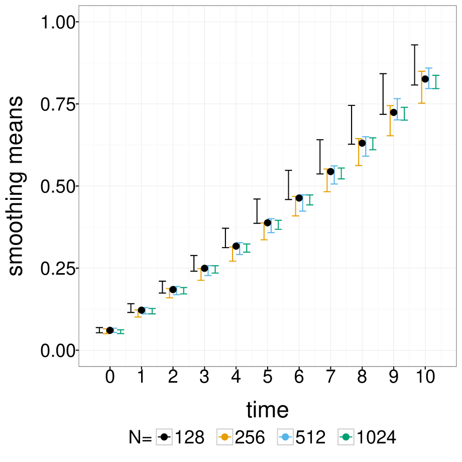
Rhee–Glynn estimators.
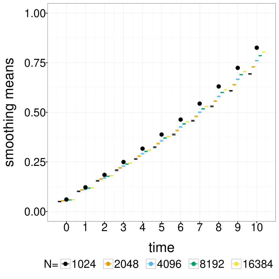
Estimators obtained by particle filters.
4 Numerical experiments in a prey-predator model
We investigate the performance of the correlated particle marginal Metropolis–Hastings algorithm and of the Rhee–Glynn smoother for a nonlinear non-Gaussian model. We consider the Plankton–Zooplankton model of Jones et al. (2010), which is an example of an implicit model: the transition density is intractable (Bretó et al., 2009; Jacob, 2015). The hidden state represents the population size of phytoplankton and zooplankton, and the transition from time to is given by a Lotka–Volterra equation,
where the stochastic daily growth rate is drawn from at every integer time . The propagation of each particle involves solving numerically the above equation, here using a Runge-Kutta method in the odeint library (Ahnert and Mulansky, 2011). The initial distribution is given by and . The parameters and represent the clearance rate of the prey and the growth efficiency of the predator. Both and parameterize the mortality rate of the predator. The observations are noisy measurements of the phytoplankton , ; is not observed. We generate observations using , , , , .
4.1 Correlated particle marginal Metropolis–Hastings
The parameter is . We specify a centered normal prior on with variance , an exponential prior on with unit rate, and uniform priors in for the four other parameters. With logarithm and logistic transforms, we map to . For the Metropolis–Hastings proposal distribution, we use a normal random walk with a covariance matrix chosen as one sixth of the covariance of the posterior, obtained from long pilot runs. We start the Markov chains at the (transformed) data-generating parameter. We then run the particle marginal Metropolis–Hastings with particles and iterations, times independently, and obtain a mean acceptance rate of , with standard deviation of , and an effective sample size averaged over the parameters (ESS) of . With only particles, we obtain a mean acceptance of () and an ESS of . Density estimators of the posterior of with these two samplers are shown on the left-most plots of Figure 13.
We investigate whether we can obtain better posterior approximations using the correlated Metropolis–Hastings algorithm, still with particles and iterations. We set the correlation coefficient for the propagation of the process-generating variables to . We consider the use of index-coupled, sorted and transport resampling. For the latter we choose and . For index-coupled resampling, we obtain an acceptance of (), with sorted resampling () and with transport resampling (). For the ESS, we obtain for index-coupled resampling, for sorted resampling and for transport resampling. We display the density estimators of the posterior of in the right-most panels of Figure 13, for index-coupled and transport resampling. Similar results are obtained with sorted resampling (not shown). However, results in Section 3.2 indicate that sorted resampling would be less efficient in higher dimension. We conclude that the correlated algorithm with particles give posterior approximations that are comparable to those obtained with a standard PMMH algorithm that uses four times more particles; thus important computational savings can be made. With the provided R implementation, the algorithm with and transport resampling takes around minutes per run, compared to minutes for the other schemes, and around minutes for the standard algorithm with .
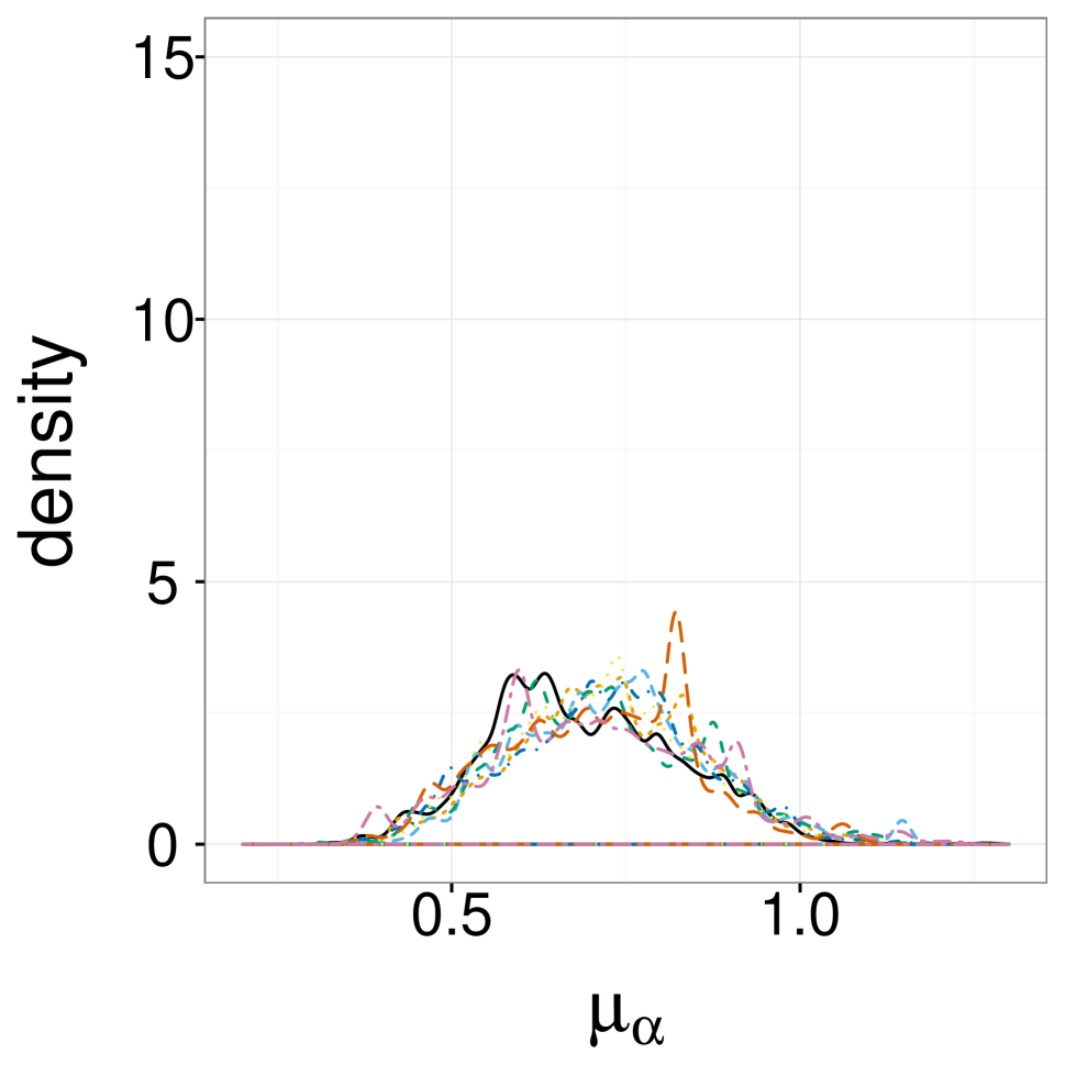
PMMH, .
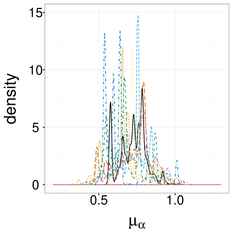
PMMH, .
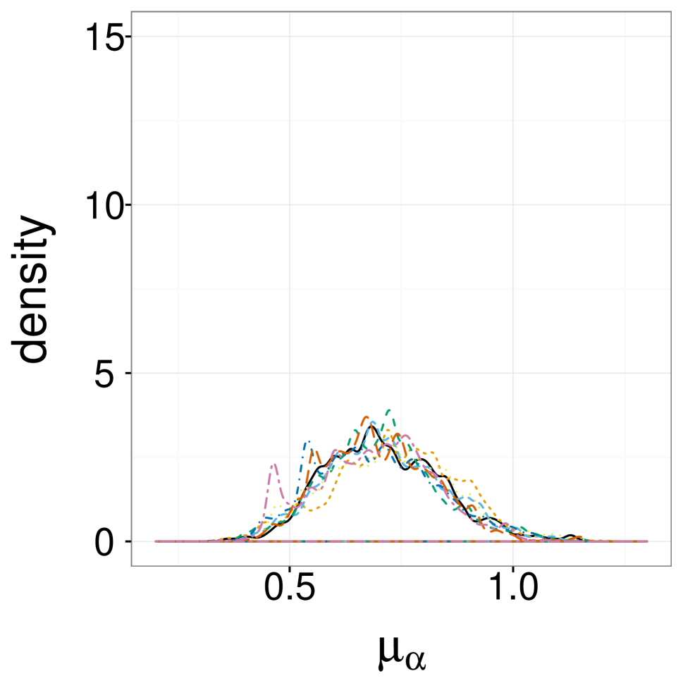
Correlated PMMH, , index-c.
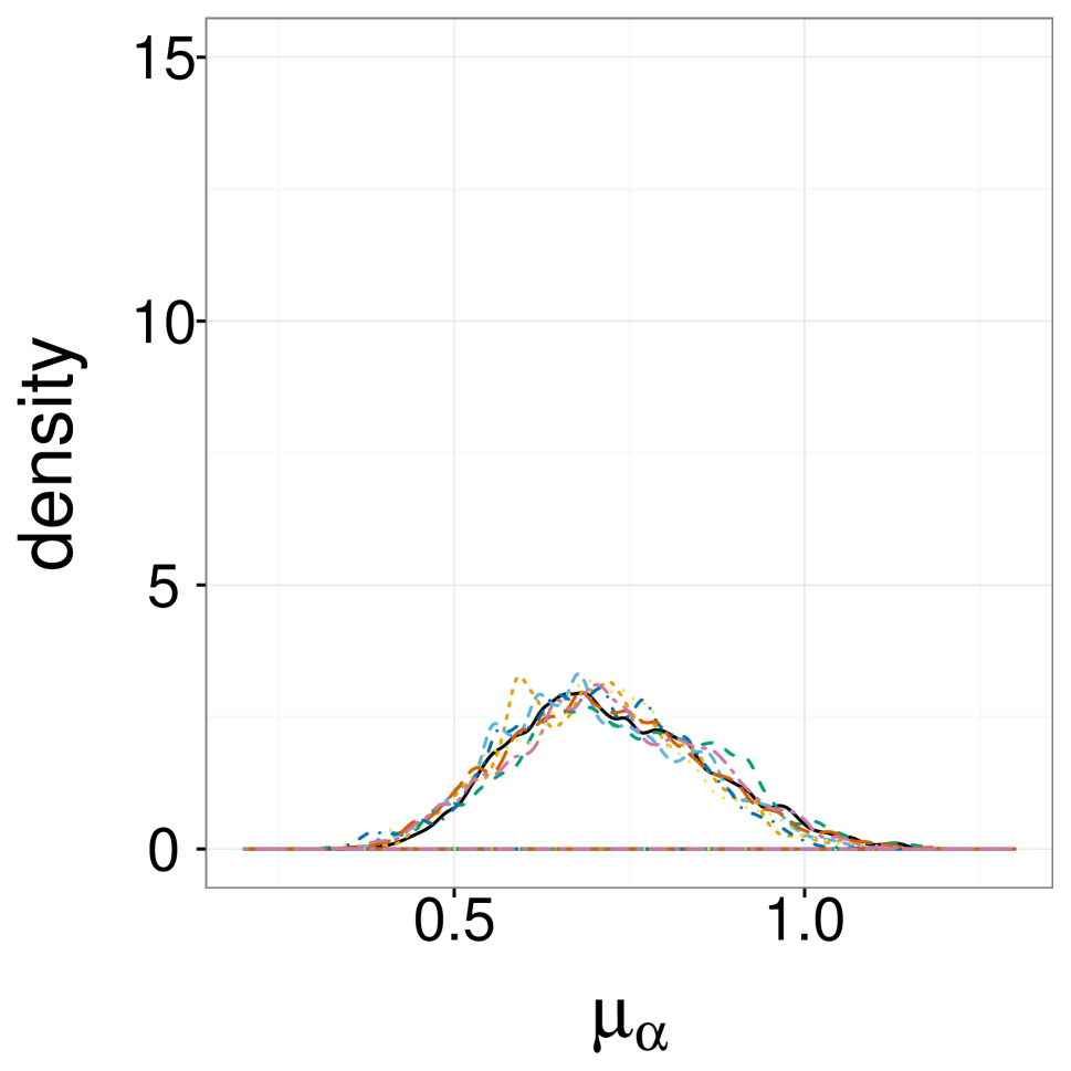
Correlated PMMH, , transport.
4.2 Rhee–Glynn smoother
Next, we consider the problem of estimating the mean population of zooplankton at each time , given a fixed parameter taken to be the data-generating one. The intractability of the transition density precludes the use of ancestor or backward sampling, or the use of forward filtering backward sampling.
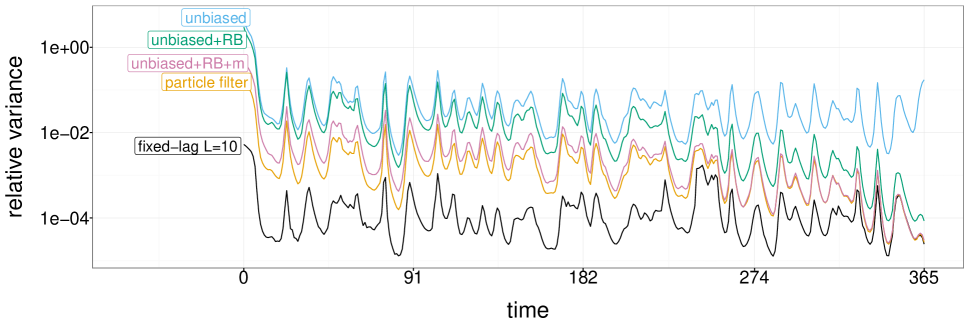
We draw independent Rhee–Glynn smoothing estimators, using particles. The observed meeting times have a median of , a mean of and a maximum of . The estimator of the smoothing mean of at each time is obtained by averaging independent estimators. We compute the Monte Carlo variance of at each time, and define the relative variance as .
We combine the Rhee–Glynn estimator (denoted by “unbiased” below) with the variance reduction technique of Section 3.3.3 (denoted by “unbiased+RB”). Furthemore, we use the variance reduction of Appendix D, denoted by “unbiased+RB+m”, with chosen to be the median of the meeting time, i.e. . The latter increases the average meeting time from to . We compare the resulting estimators with a fixed-lag smoother (Doucet and Johansen, 2011) with a lag parameter , and with a standard particle filter storing the complete trajectories.
We use the same number of particles and compute estimators for each method. The relative variance is shown in Figure 14. First we see that the variance reduction techniques have a significant effect, particularly for close to but also for small . In particular, the estimator with Rao–Blackwellization (“unbiased+RB+m”) achieves nearly the same relative variance as the particle filter. The cost of these estimators can be computed as the number of iterations , times twice the cost of a particle filter for each coupled particle filter. In the present setting where the average number of iterations is around five, we conclude that removing the bias from the standard particle filter can be done for an approximate ten-fold increase in computational cost. As expected the fixed-lag smoother leads to a significant decrease in variance. For this model, the incurred bias is negligible for (not shown), which, however, would be hard to tell if we did not have access to either unbiased methods or long runs of asymptotically exact methods.
In this model, standard particle filters and fixed-lag approximations perform well, leading to smaller mean squared error than the proposed estimators, for a given computational cost. However, the proposed estimators are competitive, the tuning of the algorithm is minimal, and unbiasedness prevents the possibility of over-confident error bars as in Section 3.3.4. Therefore the proposed method trades an extra cost for convenience and reliability.
5 Discussion
Coupled particle filters can be beneficial in multiple settings. Coupled bootstrap particle filters can be helpful in score estimation and parameter inference, while coupled conditional particle filters lead to a new smoothing algorithm. The attractive features of the Rhee–Glynn smoother include simple parallelization and accurate error bars; these traits would be shared by perfect samplers, which aim at the more ambitious task of sampling exactly from the smoothing distribution (Lee et al., 2014).
We have shown the validity of the Rhee–Glynn estimator under mild conditions, and its behaviour as a function of the time horizon and the number of particles deserves further analysis. Numerical experiments in Appendix F investigate the effect of the time horizon and of the number of particles, among other effects. Furthermore, together with Fisher’s identity (Poyiadjis et al., 2011), the proposed smoother produces unbiased estimators of the score, for models where the transition density is tractable. This could in turn help maximizing the likelihood via stochastic gradients.
Another topic of future research might be the development of coupling ideas outside the context of state space models, following the growing popularity of particle methods in varied settings (see e.g. Del Moral et al., 2006; Bouchard-Côté et al., 2012; Naesseth et al., 2014).
Appendices
Appendix A describes the sampling of a second particle filter given a first one. Appendix B provides conditions for the validity of the correlated particle marginal Metropolis–Hastings, and Appendix C for the validity of the Rhee–Glynn smoother. Appendix D describes an additional variance reduction technique for the Rhee–Glynn smoother. Appendix E provides a description of the approximation of the transport problem. Appendix F provides extensive numerical experiments for the proposed smoother and Appendix G gives pseudo-code descriptions. R functions to reproduce the figures of the article are provided at github.com/pierrejacob/ in CoupledPF and CoupledCPF.
Acknowledgements
Similar ideas and other applications of coupled resampling schemes have been independently proposed in Sen et al. (2016). The first author thanks Mathieu Gerber and Marco Cuturi for helpful discussions. This work was initiated during the workshop on Advanced Monte Carlo methods for complex inference problems at the Isaac Newton Institute for Mathematical Sciences, Cambridge, UK held in April 2014. We would like to thank the organizers for a great event which led to this work.
References
- Ahnert and Mulansky (2011) Ahnert, K. and Mulansky, M. (2011) Odeint-solving ordinary differential equations in C++. arXiv preprint arXiv:1110.3397.
- Andrieu et al. (2010) Andrieu, C., Doucet, A. and Holenstein, R. (2010) Particle Markov chain Monte Carlo (with discussion). Journal of the Royal Statistical Society: Series B (Statistical Methodology), 72, 357–385.
- Andrieu et al. (2013) Andrieu, C., Lee, A. and Vihola, M. (2013) Uniform ergodicity of the iterated conditional SMC and geometric ergodicity of particle Gibbs samplers. arXiv preprint arXiv:1312.6432.
- Andrieu and Vihola (2015) Andrieu, C. and Vihola, M. (2015) Convergence properties of pseudo-marginal Markov chain Monte Carlo algorithms. The Annals of Applied Probability, 25, 1030–1077.
- Asmussen and Glynn (2007) Asmussen, S. and Glynn, P. W. (2007) Stochastic simulation: Algorithms and analysis, vol. 57. Springer.
- Aude et al. (2016) Aude, G., Cuturi, M., Peyré, G. and Bach, F. (2016) Stochastic optimization for large-scale optimal transport. arXiv preprint arXiv:1605.08527.
- Benamou et al. (2015) Benamou, J.-D., Carlier, G., Cuturi, M., Nenna, L. and Peyré, G. (2015) Iterative Bregman projections for regularized transportation problems. SIAM Journal on Scientific Computing, 37, A1111–A1138.
- Bérard et al. (2014) Bérard, J., Del Moral, P. and Doucet, A. (2014) A lognormal central limit theorem for particle approximations of normalizing constants. Electron. J. Probab, 19, 1–28.
- Bouchard-Côté et al. (2012) Bouchard-Côté, A., Sankararaman, S. and Jordan, M. I. (2012) Phylogenetic inference via sequential Monte Carlo. Systematic Biology, 61, 579–593.
- Bretó et al. (2009) Bretó, C., He, D., Ionides, E. L. and King, A. A. (2009) Time series analysis via mechanistic models. The Annals of Applied Statistics, 319–348.
- Cappé et al. (2005) Cappé, O., Moulines, E. and Rydén, T. (2005) Inference in Hidden Markov Models. Springer-Verlag, New York.
- Cérou et al. (2011) Cérou, F., Del Moral, P. and Guyader, A. (2011) A nonasymptotic theorem for unnormalized Feynman–Kac particle models. Ann. Inst. Henri Poincarré, 47, 629–649.
- Chopin and Singh (2015) Chopin, N. and Singh, S. S. (2015) On particle Gibbs sampling. Bernoulli, 21, 1855–1883.
- Cuturi (2013) Cuturi, M. (2013) Sinkhorn distances: Lightspeed computation of optimal transport. In Advances in Neural Information Processing Systems (NIPS), 2292–2300.
- Cuturi and Doucet (2014) Cuturi, M. and Doucet, A. (2014) Fast computation of Wasserstein barycenters. In Proceedings of the 31st International Conference on Machine Learning (ICML), 685–693.
- Dahlin et al. (2015) Dahlin, J., Lindsten, F., Kronander, J. and Schön, T. B. (2015) Accelerating pseudo-marginal Metropolis–Hastings by correlating auxiliary variables. arXiv preprint arXiv:1511.05483.
- Del Moral (2004) Del Moral, P. (2004) Feynman-Kac Formulae, Genealogical and Interacting Particle Systems with Applications. New York: Springer-Verlag.
- Del Moral et al. (2006) Del Moral, P., Doucet, A. and Jasra, A. (2006) Sequential Monte Carlo samplers. Journal of the Royal Statistical Society: Series B (Statistical Methodology), 68, 411–436.
- Del Moral and Murray (2015) Del Moral, P. and Murray, L. M. (2015) Sequential monte carlo with highly informative observations. SIAM/ASA Journal on Uncertainty Quantification, 3, 969–997.
- Deligiannidis et al. (2015) Deligiannidis, G., Doucet, A. and Pitt, M. K. (2015) The correlated pseudo-marginal method. arXiv preprint arXiv:1511.04992.
- Diaconis and Freedman (1999) Diaconis, P. and Freedman, D. (1999) Iterated random functions. SIAM review, 41, 45–76.
- Douc and Cappé (2005) Douc, R. and Cappé, O. (2005) Comparison of resampling schemes for particle filtering. In Proceedings of the 4th International Symposium on Image and Signal Processing and Analysis (ISPA), 64–69.
- Doucet et al. (2001) Doucet, A., de Freitas, N. and Gordon, N. (2001) Sequential Monte Carlo methods in practice. Springer-Verlag, New York.
- Doucet and Johansen (2011) Doucet, A. and Johansen, A. (2011) A tutorial on particle filtering and smoothing: Fifteen years later. In Handbook of Nonlinear Filtering. Oxford, UK: Oxford University Press.
- Doucet et al. (2015) Doucet, A., Pitt, M., Deligiannidis, G. and Kohn, R. (2015) Efficient implementation of Markov chain Monte Carlo when using an unbiased likelihood estimator. Biometrika, 102, 295–313.
- Gerber and Chopin (2015) Gerber, M. and Chopin, N. (2015) Sequential quasi Monte Carlo. Journal of the Royal Statistical Society: Series B (Statistical Methodology), 77, 509–579.
- Glasserman and Yao (1992) Glasserman, P. and Yao, D. D. (1992) Some guidelines and guarantees for common random numbers. Management Science, 38, 884–908.
- Glynn and Rhee (2014) Glynn, P. W. and Rhee, C.-H. (2014) Exact estimation for Markov chain equilibrium expectations. J. Appl. Probab., 51A, 377–389.
- Glynn and Whitt (1992) Glynn, P. W. and Whitt, W. (1992) The asymptotic efficiency of simulation estimators. Operations Research, 40, 505–520.
- Gordon et al. (1993) Gordon, N., Salmond, J. and Smith, A. (1993) A novel approach to non-linear/non-Gaussian Bayesian state estimation. IEE Proceedings on Radar and Signal Processing, 140, 107–113.
- Guarniero et al. (2015) Guarniero, P., Johansen, A. M. and Lee, A. (2015) The iterated auxiliary particle filter. arXiv preprint arXiv:1511.06286.
- Jacob (2015) Jacob, P. E. (2015) Sequential Bayesian inference for implicit hidden Markov models and current limitations. ESAIM: Proceedings and Surveys, 51, 24–48.
- Jacob et al. (2015) Jacob, P. E., Murray, L. M. and Rubenthaler, S. (2015) Path storage in the particle filter. Statistics and Computing, 25, 487–496.
- Jasra et al. (2015) Jasra, A., Kamatani, K., Law, K. J. and Zhou, Y. (2015) Multilevel particle filter. arXiv preprint arXiv:1510.04977.
- Jones et al. (2010) Jones, E., Parslow, J. and Murray, L. (2010) A Bayesian approach to state and parameter estimation in a phytoplankton-zooplankton model. Australian Meteorological and Oceanographic Journal, 59, 7–16.
- Jun et al. (2012) Jun, S.-H., Wang, L. and Bouchard-Côté, A. (2012) Entangled Monte Carlo. In Advances in Neural Information Processing Systems (NIPS), 2726–2734.
- Kahn and Marshall (1953) Kahn, H. and Marshall, A. W. (1953) Methods of reducing sample size in Monte Carlo computations. Journal of the Operations Research Society of America, 1, 263–278.
- Kantas et al. (2015) Kantas, N., Doucet, A., Singh, S. S., Maciejowski, J. and Chopin, N. (2015) On particle methods for parameter estimation in state-space models. Statistical science, 30, 328–351.
- Lee (2008) Lee, A. (2008) Towards smooth particle filters for likelihood estimation with multivariate latent variables. Master’s thesis, University of British Columbia.
- Lee et al. (2014) Lee, A., Doucet, A. and Łatuszyński, K. (2014) Perfect simulation using atomic regeneration with application to sequential Monte Carlo. ArXiv e-prints.
- Lee and Holmes (2010) Lee, A. and Holmes, C. (2010) Comment on Particle Markov chain Monte Carlo by Andrieu, Doucet and Holenstein. Journal of the Royal Statistical Society: Series B (Statistical Methodology), 72, 357–385.
- Lee and Whiteley (2015a) Lee, A. and Whiteley, N. (2015a) Forest resampling for distributed sequential Monte Carlo. Statistical Analysis and Data Mining: The ASA Data Science Journal.
- Lee and Whiteley (2015b) — (2015b) Variance estimation and allocation in the particle filter. arXiv preprint arXiv:1509.00394.
- Lindsten et al. (2015) Lindsten, F., Douc, R. and Moulines, E. (2015) Uniform ergodicity of the particle Gibbs sampler. Scandinavian Journal of Statistics, 42, 775–797.
- Lindsten et al. (2014) Lindsten, F., Jordan, M. I. and Schön, T. B. (2014) Particle Gibbs with ancestor sampling. Journal of Machine Learning Research (JMLR), 15, 2145–2184.
- Lindsten and Schön (2013) Lindsten, F. and Schön, T. B. (2013) Backward simulation methods for Monte Carlo statistical inference. Foundations and Trends in Machine Learning, 6, 1–143.
- Lindvall (2002) Lindvall, T. (2002) Lectures on the coupling method. Courier Corporation.
- Malik and Pitt (2011) Malik, S. and Pitt, M. K. (2011) Particle filters for continuous likelihood evaluation and maximisation. Journal of Econometrics, 165, 190–209.
- McLeish (2012) McLeish, D. (2012) A general method for debiasing a Monte Carlo estimator. Monte Carlo methods and applications, 17, 301–315.
- Murray et al. (2015) Murray, L. M., Lee, A. and Jacob, P. E. (2015) Parallel resampling in the particle filter. Journal of Computational and Graphical Statistics.
- Naesseth et al. (2014) Naesseth, C. A., Lindsten, F. and Schön, T. B. (2014) Sequential Monte Carlo for graphical models. In Advances in Neural Information Processing Systems (NIPS) 27. Montreal, Quebec, Canada.
- Pitt (2002) Pitt, M. K. (2002) Smooth particle filters for likelihood evaluation and maximisation. Technical report, University of Warwick, Department of Economics.
- Poyiadjis et al. (2011) Poyiadjis, G., Doucet, A. and Singh, S. S. (2011) Particle approximations of the score and observed information matrix in state space models with application to parameter estimation. Biometrika, 98, 65–80.
- Rhee (2013) Rhee, C. (2013) Unbiased Estimation with Biased Samplers. Ph.D. thesis, Stanford University. URL: http://purl.stanford.edu/nf154yt1415.
- Rhee and Glynn (2012) Rhee, C. and Glynn, P. W. (2012) A new approach to unbiased estimation for SDE’s. In Proceedings of the Winter Simulation Conference, 17:1–17:7.
- Ruiz and Kappen (2016) Ruiz, H.-C. and Kappen, H. (2016) Particle smoothing for hidden diffusion processes: Adaptive path integral smoother. arXiv preprint arXiv:1605.00278.
- Sen et al. (2016) Sen, D., Thiery, A. and Jasra, A. (2016) On coupling particle filter trajectories. arXiv preprint arXiv:1606.01016.
- The CGAL Project (2016) The CGAL Project (2016) CGAL User and Reference Manual. CGAL Editorial Board, 4.8 edn. URL: http://doc.cgal.org/4.8/Manual/packages.html.
- Vihola (2015) Vihola, M. (2015) Unbiased estimators and multilevel Monte Carlo. arXiv preprint arXiv:1512.01022.
- Whiteley (2010) Whiteley, N. (2010) Comment on Particle Markov chain Monte Carlo by Andrieu, Doucet and Holenstein. Journal of the Royal Statistical Society: Series B (Statistical Methodology), 72, 357–385.
- Whiteley (2013) — (2013) Stability properties of some particle filters. Ann. Appl. Probab., 23, 2500–2537.
- Williams (1991) Williams, D. (1991) Probability with martingales. Cambridge university press.
Appendix A Joint or conditional sampling of particle filters
If we are interested in estimating two likelihoods and , for known values of and , we can run a coupled particle filter in one forward pass, as described in Section 2.2. Likewise, the coupled conditional particle filter given two reference trajectories can be run in one forward pass. However, we might need to correlate with for various values of which are not known in advance, as in the setting of Metropolis–Hastings schemes in Section 3.2.
To address this situation, we can run a first particle filter given , and store all the generated particles , ancestors and random numbers for all . We can later run a second particle filter, given , conditionally on the variables generated by the first filter. At each resampling step, a probability matrix is computed given the variables generated thus far. The ancestry vector is then sampled according to , conditionally upon the ancestors from the first filter. Conditional sampling from can be done in order operations for index-coupled resampling, in order for sorted resampling and in order for generic coupled resampling schemes such as transport resampling.
Storing all the generated variables incurs a memory cost of order . By carefully storing and resetting the state of the random number generator, one can in principle re-compute the first particle filter during the run of the second one, and thus the memory cost can be reduced to , in exchange of a two-fold increase in computational cost and a more sophisticated implementation (see e.g. Jun et al., 2012, for a similar discussion).
Appendix B Validity of correlated particle marginal MH
We give a sufficient condition on the coupled resampling scheme for the correlated particle marginal MH algorithm to target the same distribution as the standard particle marginal MH algorithm.
Let denote the probability distribution of the ancestors at step . Since the weights are deterministic functions of , , and , we can also write . In the proposed algorithm, and are used to compute a probability matrix and then are sampled conditionally on as described in Appendix A. We denote that conditional distribution by .
Lemma B.1.
Assume that the marginal and conditional resampling distribution, respectively and , associated with the coupled resampling scheme, are such that
| (4) |
Furthermore, assume that under the marginal resampling distribution , for all and in . Then the Markov kernel defined on , and by the correlated particle marginal MH algorithm has the same invariant distribution as the standard particle marginal MH.
We first provide the proof of Lemma B.1, and then we show that the condition of Eq. (4) is satisfied for sorted, index-coupled and transport resampling schemes.
Lemma B.1.
The extended target distribution of the particle marginal MH algorithm has density
| (5) |
which is just a change of notation compared to Andrieu et al. (2010). The condition for all and in ensures that the marginal distribution on is indeed the posterior distribtuion .
We denote by all the auxiliary variables generated by the particle filter: for all , and for all . The extended target distribution of Eq. (5) can be rewritten , where is the distribution of defined by a run of the particle filter.
Rewriting the procedure described in Section 3.2, from the state , we sample and from a Markov kernel on the space of , which may depend on and . The particle marginal MH algorithm uses . Other kernels leaving invariant can be constructed, a sufficient condition being the standard detailed balance:
| (6) |
We consider kernels of the form
In this expression, is a Markov kernel in detailed balance with respect to , the distribution of the process-generating variables. The condition of Eq. (4) implies Eq. (6). ∎
For independent and sorted resampling, the conditional sampling of does not require any variable from the first particle system, so that we have
and the condition of Eq. (4) is satisfied.
For general coupled resampling schemes, under conditional sampling, for each , is distributed according to the -th row of defined by a coupled resampling scheme, e.g. Eq. (1) for index-coupled resampling. The conditional probability takes the form . For the index-coupled probability matrix of Eq. (1), Eq. (4) is satisfied, with respect to , because we obtain the transpose of if we swap and in its construction.
For transport resampling, the distance matrix in Section 2.3 is such that we obtain its transpose if and are swapped in its construction. Thus, the optimal transport probability matrix is such that we obtain its transpose if and are swapped in its definition. Therefore, if is distributed according to for each , then the condition of Eq. (4) will be satisfied.
However, if we use an approximate solution to the transport problem, then the condition might not hold. This can be circumvented by symmetrizing the coupled resampling matrix, by computing using , and using . Then one can use the matrix , and sample distributed according to for each . This ensures that the detailed balance condition holds with respect to the multinomial resampling distribution.
Appendix C Validity of Rhee–Glynn smoothing estimators
We first state a result on the probability of meeting in one step of the coupled conditional particle filter.
Lemma C.1.
The constant depends on and , and on the coupled resampling scheme being used. Lemma C.1 can be used, together with the coupling inequality (Lindvall, 2002), to prove the ergodicity of the conditional particle filter kernel, which is akin to the approach of Chopin and Singh (2015). The coupling inequality states that the total variation distance between and is less than , where is the meeting time. By assuming , follows at each step , and we obtain a bound for the total variation distance between and . Using Lemma C.1, we can bound the probability from above by , as in the proof of Theorem 3.1 below. This implies that the computational cost of the proposed estimator has a finite expectation for all and .
C.1 Proof of Lemma C.1
Dropping the parameter from the notation, we use for the transition, for the initial distribution and for the measurement. Let denote the filtrations generated by the coupled conditional particle filter at time . We denote by , for , the surviving trajectories at time .
Let be the set of common particles at time defined by . The meeting probability, implicitly conditioned upon the reference trajectories and , can be bounded by:
| (7) |
where we have used Assumptions 1 and 2. Now, let and consider
| (8) |
since the two trajectories agree on . We have
| (9) |
and thus
| (10) |
The inner conditional expectation can be computed as
| (11) |
where we have again used Assumptions 1 and 2. Furthermore, on it holds that and therefore, combining Eqs. (8)–(11) we get
| (12) |
Thus, if we define for , , and , it follows that
where is the normalizing constant of the model, defined as where the expectation is with respect to the distribution of the latent process .
We note that, for any fixed , the bound goes to zero when . The proof fails to capture accurately the behaviour of in Lemma C.1 as a function of and .
C.2 Proof of Theorem 3.1
We present a proof for a generalization of the estimator given in Section 3.3. Introduce a truncation variable , with support on the integers . Define the estimator as
| (13) |
where and , for . We consider the following assumption on the truncation variable.
Assumption 4.
This assumption precludes the use of a range of values of near one, which could have been a tempting choice for computational reasons. On the other hand, it does not prevent the use of values of near , so that we retrieve the estimator of Eq. (3) by setting , ensuring that Assumption 4 is satisfied for all values of and .
We can first upper-bound , for all , using Lemma C.1 (see e.g. Williams (1991), exercise E.10.5). We obtain for all ,
| (14) |
This ensures that is finite; and that is almost surely finite. We then introduce the random variables
| (15) |
Since is almost surely finite, and since for all , then almost surely when . We prove that is a Cauchy sequence in , i.e. goes to as . We write
and thus, using the independence between and ,
To control , we use Hölder’s inequality, with , and , where is as in Assumption 3,
Furthermore, using Assumption 3, there exists such that, for large enough,
| (16) |
We write , and take such that . Using Cauchy–Schwarz, we have for all ,
We can now write
Under Assumption 4, we have . For the above series to go to zero when and , it is enough that . By definition of , this holds if , which is part of Assumption 4. Thus is a Cauchy sequence in .
By uniqueness of the limit, since goes almost surely to , goes to in . This shows that has finite first two moments. We can retrieve the expectation of by
according to Assumption 3. We can retrieve the second moment of by
Appendix D Further variance reduction for the Rhee–Glynn estimator
A variance reduction can be achieved in the following way. Let be two integers such that . Define
| (17) | ||||
| (18) |
We have by Eq. (18) and using the fact that and have the same distribution. Furthermore, goes to as under Assumption 3. We consider the estimator , which can be computed in a finite time as follows.
We run Algorithm 1 until step . If , from Eq. (17), almost surely, since for all . If , , again using Eq. (17). The estimator is thus made of a single term with large probability if is large enough; the computational cost is of instead of for the original estimator. The intuition is that the fewer terms there are in , the smaller the variance.
Another question is whether we can average over various choices of . We can compute where ; this estimator is still unbiased. It follows (after some calculations) that
where ; the choice of coefficients is left for future work.
Appendix E Approximate transport
In this section, we briefly describe the approximation to the transport problem introduced in Cuturi (2013); Cuturi and Doucet (2014), which is explained along with various other methods in Benamou et al. (2015). The idea is to regularize the original transport program, with the modified objective function
where is the entropy of , is the sum of the terms , and . When , minimizing the above objective over corresponds to the original optimal transport problem. We can write
where and is the element-wise exponential of . Minimizing the regularized transport objective is equivalent to finding the matrix with minimal KL projection on , leading to the optimization problem
| (19) |
Compared to the original transport problem, this program is computationally simpler. By noting that where and , we can find the solution of Eq. (19) by starting from , and by performing iterative KL projections on and , thus constructing a sequence of matrices for . When goes to infinity, the matrix converges to . This is Algorithm 1 in Cuturi (2013), which we state for completeness in Algorithm 2 below.
The algorithm is iterative, and requires matrix-vector multiplications which cost at every iteration. The number of steps to achieve a certain precision can be taken independently of the number of particles , thanks to the convexity of the objective function (Cuturi, 2013). The overall cost is thus in . Recent and future algorithms might reduce this cost, see for instance the algorithm of Aude et al. (2016).
Input: , two -vectors of normalized weights, , two sets of locations in ; a distance on .
Parameters: for the regularization, for the number of iterations.
The element-wise division between two vectors is denoted by , is a column vector of ones.
-
1.
Compute the pairwise distances where .
-
2.
Compute (element-wise) and set .
-
3.
For ,
-
(a)
,
-
(b)
.
-
(a)
-
4.
Compute as .
There are two tuning parameters: the regularization parameter and the number of iterations . For , we follow Cuturi (2013) and set a small proportion of the median of the distance matrix . For instance, we can set . For the choice of , we use the following adaptive criterion.
As described in Section 2.3, once the approximate solution is obtained by Algorithm 2, we need to correct its marginals. We compute the approximate marginals and , and set
The final transport probability matrix is given by . When increases, gets nearer to the regularized solution which is in . Accordingly, when increases we can take close to one. This gives a heuristic approach to choose : we stop Algorithm 2 when the current solution is such that computed above is at least a certain value, for instance . This ensures that the transport probability matrix is a close approximation to the regularized transport problem.
Appendix F Experiments with the Rhee–Glynn smoother
We explore the sensitivity of the proposed smoother to various inputs, section by section. The experiments are based on the hidden auto-regressive model, with , and the data are generated with ; except in Section F.6 where we use a nonlinear model. Each experiment is replicated times. We do not use any variance reduction technique in this section.
F.1 Effect of the resampling scheme
First we investigate the role of the resampling scheme. A naive scheme is systematic resampling performed on each system with a common uniform variable. A second scheme is index-coupled resampling as described in Section 2.4. In both cases, at the final step of the coupled conditional particle filter, we sample two trajectory indices using systematic resampling with a common uniform variable.
We consider a time series of length . In Table 1, we give the average meeting time as a function of , for both resampling schemes, with the standard deviation between parenthesis. First we see that the meeting time is orders of magnitude smaller when using index-coupled resampling. Secondly, we see that the meeting time tends to decrease with , when using index-coupled resampling, whereas it increases when using systematic resampling. For longer time series, we find that the index-coupled resampling is the only viable option, and thus focus on this scheme for the Rhee–Glynn smoother.
| systematic | index-coupled | |
|---|---|---|
| N = 50 | 482.87 (472.96) | 7.95 (7.41) |
| N = 100 | 462.88 (448.37) | 4.88 (3.45) |
| N = 150 | 531.69 (546.32) | 4.19 (2.68) |
| N = 200 | 569.49 (575.09) | 4.01 (2.34) |
F.2 Effect of the number of particles
We consider the effect of the number of particles , on the meeting time and on the variance of the resulting estimator. We use a time series of length , generated from the model. As seen in the previous section, when using index-coupled resampling, we expect the meeting time to occur sooner if is larger. On the other hand, the cost of the coupled conditional particle filter is linear in , so that the overall cost of obtaining each estimator has expectation of order . We give estimators of this cost as a function of in Table 2, as well as the average meeting time. We see that the cost per estimator decreases when increases, and then increases again. There seems to be an optimal value of yielding the minimum cost.
| cost | meeting time | |
|---|---|---|
| N = 256 | 220567 (241823) | 861.59 (944.62) |
| N = 512 | 17074 (17406) | 33.35 (34) |
| N = 1024 | 7458 (5251) | 7.28 (5.13) |
| N = 2048 | 8739 (4888) | 4.27 (2.39) |
| N = 4096 | 14348 (6631) | 3.5 (1.62) |
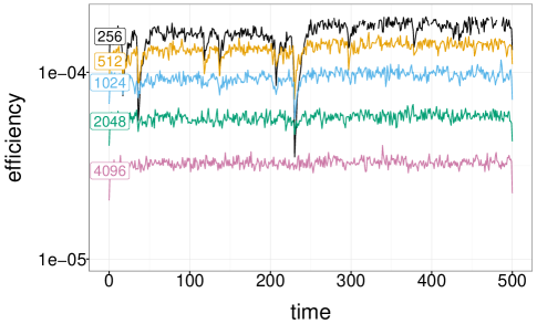
We now consider the estimators of each smoothing mean , for , i.e. we take to be the identity function. We compute the empirical variance of , for each , over the experiments. To take into account both variance and computational cost, we define the efficiency as and approximate this value for each , using the estimators. The results are shown in Figure 15.
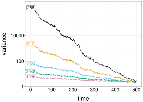
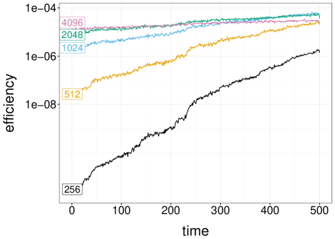
We see that the variance explodes exponentially when increases (for fixed and increasing ; see Section F.5 for the behaviour with ). From Figure 15a, the variance is reduced when larger values of are used. Secondly, the variance is most reduced for the estimators of the first smoothing means, i.e. for small . As such, the efficiency is maximized for the largest values of only when is small, as can be seen from Figure 15b. For values of closer to , the efficiency is higher for and than it is for .
F.3 Effect of the truncation variable
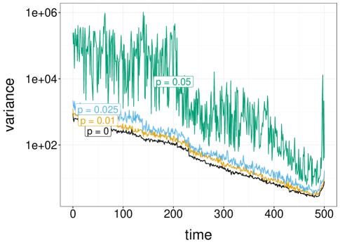
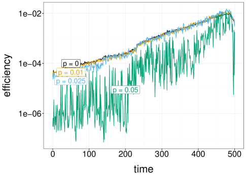
We now consider the use of Geometric truncation variables, as introduced in the Appendix C. We set and . We try a few values of the Geometric probability , in an attempt to reduce the computation cost per estimator. The value corresponds to the estimator proposed in Section 3.3. The average meeting times are shown in Table 3.
| meeting time | |
|---|---|
| p = 0 | 31.94 (31.26) |
| p = 0.025 | 17.66 (17.35) |
| p = 0.05 | 11.82 (11.68) |
We plot the variance of the estimator of the smoothing mean against on Figure 16a, for each . We plot the efficiency against on Figure 16b, for each . First, from Figure 16a, we see that increasing leads to a higher variance. In particular, the value leads to a much larger variance than the other values. This seems to be in agreement with Assumption 4, which states that has to be below a certain threshold related to the meeting probability.
On Figure 16b, we see that the increase of variance is compensated by a reduction of the computation cost, for the smaller values of . Therefore, the three smaller values lead to the same overall efficiency. On the other hand, the largest value leads to a significantly lower efficiency. Thus, there does not seem to be much benefit in using in this example.
F.4 Effect of ancestor sampling
We consider the use of ancestor sampling, which requires being able to evaluate the transition density, , for all and all . We set as before, and consider different values of . The average meeting times are displayed in Table 4. We see that the meeting times are significantly reduced by using ancestor sampling, especially for smaller numbers of particles.
| without ancestor sampling | with ancestor sampling | |
|---|---|---|
| N = 256 | 861.59 (944.62) | 8.79 (3.33) |
| N = 512 | 33.35 (34) | 5.99 (2.27) |
| N = 1024 | 7.28 (5.13) | 4.51 (1.88) |
| N = 2048 | 4.27 (2.39) | 3.76 (1.63) |
| N = 4096 | 3.5 (1.62) | 3.34 (1.51) |
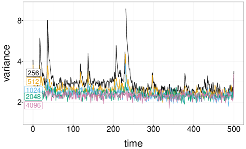
We consider variance and efficiency, here defined as . The results are shown in Figure 17. This is to be compared with Figure 15 obtained without ancestor sampling.
First we see that the variance is significantly reduced by ancestor sampling. The variance seems to increase only slowly as increases, for each value of . From Figure 17b, we see that the smallest value of now leads to the most efficient algorithm. In other words, for a fixed computational budget, it is more efficient to produce more estimators with than to increase the number of particles and to average over fewer estimators.
F.5 Effect of the time horizon
We investigate the effect of the time horizon , that is, the total length of the time series, on the performance of the smoother. We expect the conditional particle filter kernel to perform less and less well when increases. To compensate for this loss of efficiency, we increase the number of particles linearly with : for we use , for we use , and so forth up to and . With that scaling, the computational cost of each run of coupled conditional particle filter is quadratic in . A first question is whether the meeting time is then stable with . Table 5 reports the average meeting times obtained when scaling linearly with . We see that the meeting times occur in roughly the same number of steps, implying that the linear scaling of with is enough.
| without ancestor sampling | with ancestor sampling | |
|---|---|---|
| N = 128, T = 64 | 11.73 (10.87) | 6.54 (3.91) |
| N = 256, T = 128 | 9.51 (7.61) | 5.77 (2.8) |
| N = 512, T = 256 | 11.25 (9.33) | 5.66 (2.67) |
| N = 1024, T = 512 | 7.8 (6.05) | 4.51 (1.81) |
| N = 2048, T = 1024 | 9.07 (6.82) | 4.58 (1.9) |
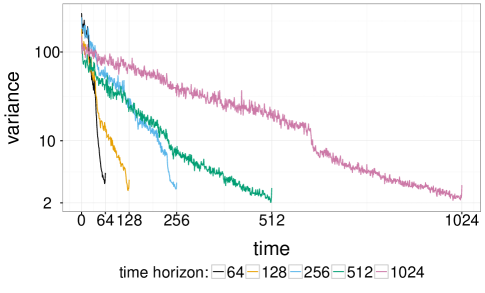
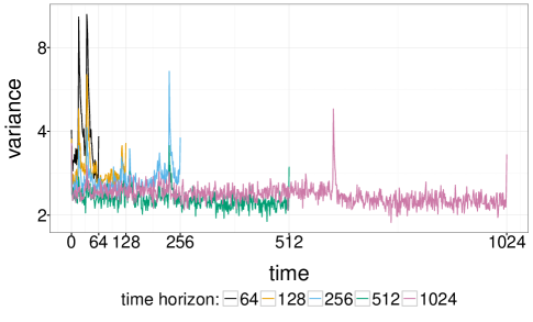
A second question is whether scaling linearly with is enough to ensure that the variance of the resulting estimator is stable. Results are shown in Figure 18, obtained without (Figure 18a) and with ancestor sampling (Figure 18b). The plots show the variance of the estimator of the smoothing means for all and various . We see that, for the values of that are less than all the time horizons, the variance of the estimators of seems stable with . The experiments thus indicate that, to estimate for all , one can scale linearly in and expect the meeting time and the variance of the Rhee–Glynn estimators to be stable. Overall, the computational cost is then quadratic in .
F.6 Effect of multimodality in the smoothing distribution
We switch to another model to investigate the behaviour of the Rhee–Glynn estimator when the smoothing distribution is multimodal. We consider the nonlinear growth model used by Gordon et al. (1993). We set , and, for ,
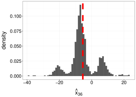
where and are independent normal variables, with variances and respectively. We generate observations using , following Gordon et al. (1993). Because the measurement distribution depends on through , the sign of is hard to identify, and as a result the smoothing distribution has multiple modes. We run a conditional particle filter with ancestor sampling, with particles for iterations, and discard the first iterations. We plot the histogram of the obtained sample for at time in Figure 19a. We notice at least two modes, located around and , with possibly an extra mode near zero.

We run the Rhee–Glynn smoother with and ancestor sampling. Each estimator took less than iterations of the coupled conditional particle filter to meet, with a median meeting time of iterations. The total number of calls to the coupled conditional particle filter to obtain estimators adds up to . We plot the histogram of the estimators , for , of the smoothing mean at time in Figure 19b. We see that the distribution of the estimator is itself multimodal. Indeed, the two initial reference trajectories might belong to the mode around , or to the mode around , or each trajectory might belong to a different mode. Each of these cases leads to a mode in the distribution of the Rhee–Glynn estimator.
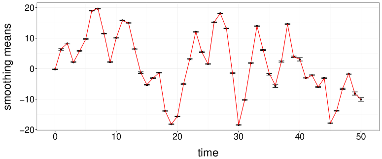
The resulting estimator of each smoothing mean is obtained by averaging the independent estimators . We compute the Monte Carlo standard deviation at each time , and represent the confidence intervals as error bars in Figure 20. The line represents the smoothing means obtained by conditional particle filter with ancestor sampling, taken as ground truth. The agreement shows that the proposed method is robust to multimodality in the smoothing distribution.
Appendix G Pseudo-code for particle filters
We provide pseudo-code for the bootstrap particle filter (Algorithm 3), the conditional particle filter (Algorithm 4), the coupled bootstrap particle filter (Algorithm 5), and the coupled conditional particle filter (Algorithm 6).
At step .
-
1.
Draw , for all .
This can also be written , for all . -
2.
Set , for all .
At step .
-
1.
Draw ancestors .
-
2.
Draw , for all .
This can also be written , for all . -
3.
Compute , for all , and normalize the weights.
Return the likelihood estimator .
At step .
-
1.
Draw , for , and set .
This can also be written , for all , and . -
2.
Set , for .
At step .
-
1.
Draw ancestors , and set .
-
2.
Draw , for all , and set .
This can also be written , for all , and . -
3.
Compute , for all , and normalize the weights.
Draw a trajectory.
-
1.
Draw from a discrete distribution on , with probabilities .
-
2.
For , set .
Return .
At step .
-
1.
Draw , and compute and , for all .
-
2.
Set and , for all .
At step .
-
1.
Compute a probability matrix , with marginals and . Sample from , for all .
-
2.
Draw , and compute and , for all .
-
3.
Compute and , for all , and normalize the weights.
Return and .
At step .
-
1.
Draw , compute and for .
-
2.
Set and .
-
3.
Set and , for .
At step .
-
1.
Compute a probability matrix , with marginals and . Sample from , for all . Set and .
-
2.
Draw , and compute and , for all . Set and .
-
3.
Compute and , for all , and normalize the weights.
Draw a pair of trajectories.
-
1.
Compute a probability matrix , with marginals and . Draw from .
-
2.
For , set and .
Return and .