THE BELIEF NOISY-OR MODEL APPLIED TO NETWORK RELIABILITY ANALYSIS

Abstract

One difficulty faced in knowledge engineering for Bayesian Network (BN) is the quantification step where the Conditional Probability Tables (CPTs) are determined. The number of parameters included in CPTs increases exponentially with the number of parent variables. The most common solution is the application of the so-called canonical gates. The Noisy-OR (NOR) gate, which takes advantage of the independence of causal interactions, provides a logarithmic reduction of the number of parameters required to specify a CPT. In this paper, an extension of NOR model based on the theory of belief functions, named Belief Noisy-OR (BNOR), is proposed. BNOR is capable of dealing with both aleatory and epistemic uncertainty of the network. Compared with NOR, more rich information which is of great value for making decisions can be got when the available knowledge is uncertain. Specially, when there is no epistemic uncertainty, BNOR degrades into NOR. Additionally, different structures of BNOR are presented in this paper in order to meet various needs of engineers. The application of BNOR model on the reliability evaluation problem of networked systems demonstrates its effectiveness.

1 Introduction

Bayesian Network (BN) is a probabilistic graphical model that represents a set of random variables and their conditional dependencies via a directed acyclic graph (DAG) ¹. BN can be used to learn causal relationships and gain understanding of a problem domain. It allows probabilistic beliefs to be updated automatically when new information becomes available. BN is also able to represent multi-attribute correlated variables and to perform relevant simulations or diagnoses. Owing these advantages, it has been widely applied on the problem of reliability or safety analysis for both static and dynamic systems ²; ³; ⁴; ⁵.

In BN, Conditional Probability Tables (CPTs) should be defined to measure the relationships between variables. However, it has been pointed out that it is usually difficult to quantify the CPTs due to the complexity ⁶. One of the most appropriate solutions to this problem is the Noisy-OR (NOR) gate, which can be attributed to Pearl ⁷. Traditional NOR can only deal with the binary variables. Srinivas ⁸ extended NOR for $n$-ary input and output variables, and arbitrary functions other than Boolean OR function can be used. But it has not taken into account the uncertainty on parameters and the state which often exists in practice. Considering such uncertainty, Fallet et al. ⁹ proposed the imprecise extensions of Noisy OR (ImNOR) thereafter. Nevertheless, there are still some problems for ImNOR which will be discussed in detail later.

The theory of belief functions, also called Dempster–Shafer Theory (DST), offers a mathematical framework for modeling uncertainty and imprecise information ¹⁰. Belief functions are widely employed in various fields, such as data classification ^{11; 12; 13}, data clustering ^{14; 15; 16; 17}, social network analysis ^{18; 19; 20; 21} and statistical estimation ^{22; 23; 24}. The concept of evidential networks, which is a combination of belief function theory and Bayesian network, is proposed to model system reliability with imprecise knowledge ^{25; 26}. Recently, Yaghlane and Mellouli ²⁷ presented another definition of evidential networks based on Transferable Belief Model (TBM) ²⁸, Dempster-Shafer rule of combination, and binary joint trees.

The objective of this work is to enrich the existing NOR structures by integrating several types of uncertainty. Under the framework of belief functions, the Belief Noisy-OR (BNOR) model is put forward. The uncertainty of variable states can be expressed by the power set of discernment frame. The uncertainty of parameters is described by probability intervals based on which the basic belief assignments are determined. The model can model causal connections among variables as well as taking random and epistemic uncertainty into account. The proposed BNOR model can be implemented in evidential networks ²⁶, and belief reasoning is proceeded through evoking junction tree inference algorithms ²⁵; ²⁶.

The remainder of this paper is organized as follows. In Section 2, the basic knowledge about Noisy-OR gate and Dempster–Shafer theory is briefly introduced. The BNOR model is presented in detail in Section 3. In order to show the effectiveness of BNOR in real practice, Section 4 discusses about how to apply BNOR on the problem of network reliability evaluation. Conclusions are drawn in the final section.

2 Background

In this section some related preliminary knowledge will be presented. The definition of Noisy-OR gate will be described first, then some basis of belief function theory will be recalled.

2.1 Noisy-OR model

The Noisy-OR structure was introduced by Pearl ⁷ to reduce the elicitation effort in building a Bayesian network. The general properties of the Noisy-OR function and its generalizations were captured by Heckerman and Breese ²⁹ in their definition of causal independence.

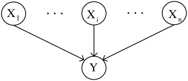
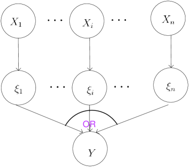
a. causal connections

b. Noisy-OR model

Figure 1: The causal connections network.

Let us consider a binary variable $Y$ with $n$ binary parent variables $X_{i}$ (see Figure 1-a). These variables can be either “True” $(T)$ or “False” $(F)$. Each $X_{i}$ exerts its influence on $Y$ independently. To build a Bayesian network, $X$ must be associated with a probability distribution $p(Y|X_{1},\cdots,X_{n})$. The number of independent parameters included in the complete specification of $p(Y|X_{1},\cdots,X_{n})$ is $2^{n}$. The Noisy-OR function is an attractive way where we can use fewer parameters to specify $p(Y|X_{1},\cdots,X_{n})$. The idea is to start with $n$ probability values $p_{i}$, which is the probability that $\{Y=T\}$ conditional on $\{X_{i}=T\}$ and $\{X_{j}=F\}$ for $j\neq i$, i.e.,

$$p_{i}=p\left\{Y=T\middle|X_{i}=T,\left\{X_{j}=F\right\}^{n}_{j=1,j\neq i}\right\}.$$ (1)

Probability $p_{i}$ is often called “link probability” and illustrates the fact that the causal dependency between $X_{i}$ and $Y$ can be inhibited. If the state of variable $X_{i}$ is $T$, then there is chance $1-p_{i}$ that it is flipped to $F$; If $X_{i}$ is $F$, then it stays with $F$. Denote the result of flipping (or not) $X_{i}$ by $\xi_{i},i=1,2,\cdots,n$ (see Figure 1-b), then

$$p(Y=\alpha|X_{1,}X_{2},\cdots,X_{n})=\sum_{\alpha_{1}\vee\cdots\vee\alpha_{n}=\alpha}p(\xi_{1}=\alpha_{1}|X_{1})\cdots p(\xi_{n}=\alpha_{n}|X_{n}),$$ (2)

where the values of $\alpha,\alpha_{i}$ are either $T$ or $F$. A Noisy-OR function is thus a disjunction of “noisy” versions of $X_{i}$ ³⁰. Let $\bm{X}_{T}$ be the set of $X_{i}$ whose state is “True”, and $\bm{X}_{F}$ be the set of $X_{i}$ which are “False”. The distribution of $Y$ conditional on $X_{1},X_{2},\cdots,X_{n}$ is

$$p\left(Y=T\middle|X_{1},X_{2},\cdots,X_{n}\right)=1-\prod_{i:X_{i}\in\bm{X}_{T}}(1-p_{i}).$$ (3)

We can see the number of independent parameters required for the conditional probability function is reduced from $2^{n}$ to $2n$ ³¹. The following example shows how to create CPTs by the use of NOR gate.

Example 1. Let us consider the Alarm System (see Figure 2). Both a burglar ($B$) and an earthquake ($E$) can set the alarm ($A$) off but neither always do so. The mechanism of the burglar and earthquake is different, thus they can be regarded as independent causes. Variable $B^{{}^{\prime}}$ (respectively, $E^{{}^{\prime}}$) describes the result after flipping (or not) of $B$ (respectively, $E$). Assume all variables are binary with values $\{T,F\}$, where $T$ represents the corresponding event happens, while $F$ means not.

Apparently, $A$ is $F$ only if both the occurrence of burglar and earthquake do not evoke the alarm due to inhibition. Using the Noisy-OR model, we can get,

$$p(A=F|B,E)=\prod_{i\in\bm{X}_{T}}(1-p_{i}),$$ (4)

The conditional probability on $\{A=T\}$ can be obtained easily:

$$p(A=T|B,E)=1-\prod_{i\in X_{T}}(1-p_{i}).$$ (5)

The following CPT can be got using Eqs. (4) and (5).

Table 1: The conditional probability table.

B	E	$A=T$	$A=F$
T	T	$1-(1-p_{1})(1-p_{2})$	$(1-p_{1})(1-p_{2})$
T	F	$p_{1}$	$1-p_{1}$
F	T	$p_{2}$	$1-p_{2}$
F	F	0	1

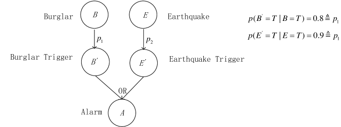
Figure 2: The alarm network.

2.2 Belief function theory

To apply the theory of belief functions, we consider a set of $q$ mutually exclusive & exhaustive elements, called the frame of discernment, defined by

$$\Theta=\{\theta_{1},\theta_{2},\cdots,\theta_{q}\}.$$ (6)

Let $X$ be a variable taking values in $\Theta$. The function $m:2^{\Theta}\rightarrow[0,1]$ is said to be the basic belief assignment (bba) on $\text{2}^{\Theta}$, if it satisfies:

$$\sum_{A\subseteq\Theta}m(A)=1,$$ (7)

and

$$m(\emptyset)=0.$$ (8)

The constraint on $\emptyset$ defined by Eq. (8) is not mandatory. It assumes that one and only one element in $\Theta$ is true (closed-world assumption). In the case where $m(\emptyset)\neq 0$, the model accepts that none of the elements could be true (open-world assumption) ²⁸. The closed-world assumption is accepted hereafter. Every $A\in 2^{\Theta}$ such that $m(A)>0$ is called a focal element. Uncertain and imprecision knowledge about the actual value of $X$ can be represented by a bba distributed on $2^{\Theta}$:

$$\bm{M}_{X}=\left[m\left(A_{1}\right),m\left(A_{2}\right),\cdots,m\left(A_{2^{q}-1}\right)\right],$$ (9)

where $A_{1},A_{2},\cdots,A_{2^{q}-1}$ are the elements of $2^{\Theta}$ arranged by natural order.

The credibility and plausibility functions are derived from a bba $m$ as in Eqs. (10) and (11).

$$Bel\text{(}A\text{)}=\sum_{B\subseteq A}m\text{(}B\text{)},~{}~{}\forall A\subseteq\Theta,$$ (10)

$$Pl\text{(}A\text{)}=\sum_{B\cap A\neq\emptyset}m\text{(}B\text{)},~{}~{}\forall A\subseteq\Theta.$$ (11)

$Bel(A)$ measures the minimal belief on $A$ justified by available information on $B(B\subseteq A)$ , while $Pl(A)$ is the maximal belief on $A$ justified by information on $B$ which are not contradictory with $A$ ($A\cap B\neq\emptyset$). The bba can be recovered from credibility functions through the fast Möbius transformations ³²:

$$m(A)=\sum_{B\subseteq A}(-1)^{|A-B|}Bel(B),\forall A\subseteq\Theta$$ (12)

The relations between $Bel$ and $Pl$ can be established as follows:

$$Bel…(A)=1-Pl(\overline{A})~{}~{},~{}~{}Pl(…A)=1-Bel…(\overline{A}),$$ (13)

where $\overline{A}$ denotes the complementary set of $A$. $Bel(\overline{A})$ is often called the doubt in $A$. Let $Pr(A)$ denote the probability of the hypothesis $A$, it is easy to get:

$$Bel(A)\leq Pr(A)\leq Pl(A).$$ (14)

Probability $Pr(A)$ belongs to the interval $[Bel(A),Pl(A)]$ but its exact value remains unknown. The bounding property (14) has been well defined in the work of Shafer ¹⁰.

Ferson et al. ³³ argued that each Dempster-Shafer structure specifies a unique probability-box (p-box), and that each p-box specifies an equivalent class of Dempster-Shafer structure ²⁶. P-boxes are sometimes considered as a granular approach of imprecise probabilities ³⁴, which are arbitrarily sets of probability distributions. Probability interval $[\underline{P}(A),\overline{P}(A)]$, which is the restricted case of p-box ²⁶, can also be used to describe the imprecision of a probability measure. The relation between a probability interval and a bba can be directly obtained ²⁶:

$$[\underline{P}(A),\overline{P}(A)]=[Bel(A),Pl(A)].$$ (15)

Belief functions can be transformed into probability distribution functions by Smets method ³⁶, where each mass of belief $m(A)$ is equally distributed among the elements of $A$. This leads to the concept of pignistic probability, $BetP$. For all $\theta_{i}\in\Theta$, we have

$$BetP(\theta_{i})=\sum_{A\subseteq\Theta|\theta_{i}\in A}\frac{m(A)}{|A|(1-m(\emptyset))},$$ (16)

where $|A|$ is the cardinality of set $A$ (number of elements of $\Theta$ in $A$). Pignistic probabilities can help us make a decision.

3 Belief Noisy-OR model

We start with the discussion of the uncertainty problem in NOR model. One of the existing approaches to express the uncertain information in NOR is the ImNOR model proposed by Fallet et al. ⁹. We will analyze the drawbacks of ImNOR and present a new NOR gate using the theory of belief functions.

3.1 The uncertainty problem in NOR structure

From an industrial point of view, it is classically accepted that observations made on the system are partially realized ³⁵. For example, it is difficult to determine whether an earthquake has happened, especially when the magnitude is small and the hypo-center is deep. In such a case, there is some uncertainty on the state of boolean parent variables and it is intuitive for experts to give a positive belief on the ignorant modality $\left\{T,F\right\}$. Simon and Weber ²⁶ have investigated a solution based on evidential network and the theory of belief functions to take into account the uncertainty on the state of binary parent variables in AND/OR gates. Simon et al. ²⁵ combined belief function theory with Bayesian reasoning to deal with this type of epistemic uncertainty. Based on Simon and Weber’s modelling formalization, Fallet et al. ⁹ proposed imprecise extensions of the Noisy-OR (ImNOR) structure to deal with the uncertainty on the state of variables and link probabilities.

ImNOR describes the uncertainty on variable state and link probabilities separately by calculating the lower bounds of the conditional probability $P\left(X\middle|\text{Pa}(X)\right)$, where $\text{Pa}(X)$ denotes the parent nodes of $X$. Consider the causal network shown in Figure 1-a. As before, the discernment frame of each variable is $\left\{T,F\right\}$, and each $X_{i}$ is interpreted as an independent “cause” of $Y$. We can express our epistemic uncertainty on variables’ state by assigning the basic belief to ignorant modality $\left\{T,F\right\}$. This modality indicates that the variable is exclusively in $\{T\}$ or $\{F\}$ state without distinguishing exactly in which state it is ⁹. Different from Noisy-OR model, in ImNOR, each active $X_{i}$ can evoke $Y$ with unknown probability $p_{i}\in[p_{iL},p_{iU}]$, where $p_{iU}-p_{iL}$ measures the degree of uncertainty on our knowledge of inhibition. Fallet provided us the formulas (see Eqs. (17)–(19)) to calculate the conditional belief mass functions:

$$m(Y=\{T\}|X_{1},X_{2},\cdots,X_{n})=1-\prod_{\{i:X_{i}=\{T\}\}}(1-p_{iL}),$$ (17)

$$m(Y=\{F\}|X_{1},X_{2},\cdots,X_{n})=\prod_{\{i:X_{i}=\{T\}\}}(1-p_{iU})\prod_{\{i:X_{i}=\text{$\left\{T,F\right\}$ }\}}(1-p_{iU}),$$ (18)

$$m(Y=\text{$\left\{T,F\right\}$ }|X_{1},X_{2},\cdots,X_{n})=\prod_{\{i:X_{i}=\{T\}\}}(1-p_{iL})-\prod_{\{i:X_{i}=\{T\}\}}(1-p_{iU})\prod_{\{i:X_{i}=\text{$\left\{T,F\right\}$ }\}}(1-p_{iU}).$$ (19)

From Eq. (17), we can get:

$$m\left(Y=\{T\}\middle|X_{1}\cdots X_{k}=\left\{T,F\right\}\cdots X_{n}\right)=1-\prod_{\{i:X_{i}=\{T\},i\in\{1,2,\cdots,k-1,k+1,\cdots,n\}\}}(1-p_{iL}),$$ (20)

and

$$m\left(Y=\{T\}\middle|X_{1}\cdots X_{k}=\left\{F\right\}\cdots X_{n}\right)=1-\prod_{\{i:X_{i}=\{T\},i\in\{1,2,\cdots,k-1,k+1,\cdots,n\}\}}(1-p_{iL}).$$ (21)

It can be seen that the belief on the proposition that “variable $Y$ is $\{T\}$” does not change when some prior precise information about the parent variables becomes available (The state of $X_{k}$ changes from $\{T,F\}$ to $\{T\}$):

$$m(Y=\{T\}|X_{1},\cdots,X_{i}=\{T,F\},\cdots X_{n})=m(Y=\{T\}|X_{1},\cdots,X_{i}=\{F\},\cdots,X_{n}).$$ (22)

Besides, there is another defect for the above method when calculating the belief mass on the conditional events where there is no working components $(X_{i}\neq T,i=1,2,\cdots,n)$. For example, when we want to know

$$m(Y|X_{i}=\{F\},i=1,2,\cdots,n-1,X_{n}=\left\{T,F\right\}),$$

the following conditional belief mass functions can be got by Eq. (18):

$$m(Y=\{F\}|X_{i}=\{F\},i=1,2,\cdots,n-1,X_{n}=\left\{T,F\right\})=1-P_{nU},$$ (23)

$$m(Y=\{F\}|X_{i}=\text{\{T,F\}},i=1,2,\cdots,n-1,X_{n}=\left\{T,F\right\})=P_{nU}.$$ (24)

As can be seen, the lower bound of probability $p_{n}$, $p_{nL}$, has no effect on the final results. That is to say, the conditional belief mass assignment remains unchanged once the upper bound of $p_{n}$ is fixed no matter how long the uncertain interval is. This is against our common sense. Since the length of the interval measures the degree of uncertainty on the available information, the longer the interval is, more mass value should be given to the ignorant state $\{T,F\}$.

3.2 Belief Noisy-OR structure

We introduce here the Belief Noisy-OR structure to express the epistemic uncertainty on the state of the variables and link probabilities at the same time. Consider the causal network where $X_{i},i=1,2,\cdots,n$ are the parents of $Y$ (Figure 1-a).

Let us first discuss the uncertainty on link probability $p_{i}$. This parametric uncertainty can be modeled by an interval $[p_{iL},p_{iU}]$, with $0\leq p_{iL}\leq p_{i}\leq p_{iU}\leq 1$. Thus the inhibition probability interval of $X_{i}$ is $[1-p_{iU},1-p_{iL}]$. In order to use evidential reasoning, the probability intervals should be transformed to belief function structures. For convenience, $n$ auxiliary variables, $X_{i}^{{}^{\prime}},i=1,2,\cdots,n$ are introduced to represent the result of flipping or not $X_{i}$. From the boundary property of belief functions (Eq. (14)), we can get

$$Bel(X_{i}^{{}^{\prime}}=\{T\}|X_{i}=\{T\})=p_{iL},$$ (25)

$$Pl(X_{i}^{{}^{\prime}}=\{T\}|X_{i}=\{T\})=p_{iU},$$ (26)

The associated belief mass distribution can be easily determined by Eq. (12). The corresponding conditional bba in $2^{\Theta}$ can be defined as:

$$m(X_{i}^{{}^{\prime}}=\{T\}|X_{i}=\{T\})=Bel(X_{i}^{{}^{\prime}}=\{T\}|X_{i}=\{T\})=p_{iL},$$ (27)

$$m(X_{i}^{{}^{\prime}}=\{F\}|X_{i}=\{T\}) =Bel(X_{i}^{{}^{\prime}}=\{F\}|X_{i}=\{T\})$$ (28)

$$=1-Pl(X_{i}^{{}^{\prime}}=\{T\}|X_{i}=\{T\})$$ (29)

$$=1-p_{iU},$$ (30)

and

$$m(X_{i}^{{}^{\prime}}=\text{$\left\{T,F\right\}$ }|X_{i}=\{T\})=p_{iU}-p_{iL},$$ (31)

where Eq. (29) is obtained by the relation between $Bel$ and $Pl$. Eqs. (27)–(31) express the uncertain knowledge of link probabilities and variable states together in the form of belief mass distributions.

When $X_{i}=\{F\}$, $Y$ is sure to stay in state $\{F\}$ . Thus the bba conditioned $X_{i}=\{F\}$ is easy to determine:

$$m(X_{i}^{{}^{\prime}}=\{T\}|X_{i}=\{F\})=0,$$ (32)

$$m(X_{i}^{{}^{\prime}}=\{F\}|X_{i}=\{F\})=1,$$ (33)

$$m(X_{i}^{{}^{\prime}}=\text{\{T,F\}}|X_{i}=\{F\})=0.$$ (34)

However, the bba on the condition $X_{i}=\text{\{T,F\}}$ is more complicated. The following equations with unknown parameters $\alpha,\beta,\gamma~{}(\alpha+\beta+\gamma=1)$ are first given, and then the methods for designing the three parameters will be discussed later.

$$m(X_{i}^{{}^{\prime}}=\text{$\{T\}$}|X_{i}=\text{$\left\{T,F\right\}$})=\alpha,$$ (35)

$$m(X_{i}^{{}^{\prime}}=\text{$\left\{F\right\}$}|X_{i}=\text{$\left\{T,F\right\}$})=\beta,$$ (36)

$$m(X_{i}^{{}^{\prime}}=\text{$\left\{T,F\right\}$}|X_{i}=\text{$\left\{T,F\right\}$})=\gamma.$$ (37)

Eqs. (35)–(37) show that in BNOR, the belief on the uncertain state $X_{i}=\{T,F\}$ may be flipped into all the possible states by different ratios. Parameters $\alpha,\beta,\gamma$ are adjustable.

Generally, the values of $\alpha,\beta,\gamma$ can be given by the proportions of belief mass on $X_{i}=\{T,F\}$ which may be transferred to $X_{i}=\{T\}$ (noted by $\lambda_{1}$, $0\leq\lambda_{1}\leq 1$), $X_{i}=\{F\}$ (noted by $\lambda_{2}$, $0\leq\lambda_{2}\leq 1$) and $X_{i}=\{T,F\}$ (noted by $\lambda_{3}$, $0\leq\lambda_{3}\leq 1$) ($\lambda_{1}+\lambda_{2}+\lambda_{3}=1$) respectively:

$$\alpha=\lambda_{1}m(X_{i}^{{}^{\prime}}=\text{$\{T\}$}|X_{i}=\text{$\{T\}$})=\lambda_{1}p_{iL},$$ (38)

$$\beta=\lambda_{1}m(X_{i}^{{}^{\prime}}=\text{$\{F\}$}|X_{i}=\text{$\{T\}$})+\lambda_{2}=\lambda_{1}(1-p_{iU})+\lambda_{2},$$ (39)

$$\gamma=\lambda_{1}m(X_{i}^{{}^{\prime}}=\text{$\left\{T,F\right\}$}|X_{i}=\text{$\{T\}$})+\lambda_{3}=\lambda_{1}(p_{iU}-p_{iL})+\lambda_{3}.$$ (40)

Parameter $\lambda_{3}$ in Eq. (40) indicates the uncertainty on the state of $X_{i}$, and it should be in direct proportion to $m(X_{i}=\{T,F\})\triangleq\eta$. It is easy to know that if $\eta\neq 0$, $\lambda_{3}\neq 0$. For simplicity, let $\lambda_{3}=\eta$ and $\lambda_{1}=\lambda$, $\lambda_{2}=1-\lambda-\eta$, then,

$$\alpha=\lambda m(X_{i}^{{}^{\prime}}=\text{$\{T\}$}|X_{i}=\text{$\{T\}$})=\lambda p_{iL},$$ (41)

$$\beta=\lambda m(X_{i}^{{}^{\prime}}=\text{$\{F\}$}|X_{i}=\text{$\{T\}$})+(1-\lambda-\eta)=\lambda(1-p_{iU})+(1-\lambda-\eta),$$ (42)

$$\gamma=\lambda m(X_{i}^{{}^{\prime}}=\text{$\left\{T,F\right\}$}|X_{i}=\text{$\{T\}$})+\eta=\lambda(p_{iU}-p_{iL})+\eta.$$ (43)

This is similar to the optimistic coefficient method in the decision theory. So we call this general approach Optimistic coefficient-BNOR (OCBNOR), where $\lambda~{}(0\leq\lambda\leq 1)$ is the optimistic coefficient.

Note that Eqs. (41)–(43) propagate the uncertainty on variable state and link probabilities simultaneously. The ignorant modality $\Theta=\{T,F\}$ represents the uncertainty on the state and the belief mass assignment $m(X_{i}^{{}^{\prime}}|X_{i})$ deals with the uncertain information of link probabilities.

Different $\lambda$ values can be set to obtain results under various requirements. For instance, if we want to make an optimistic decision, the belief to $X_{i}=\{T,F\}$ could transferred to $X_{i}^{{}^{\prime}}=\{T\}$ as most as possible. Let $\lambda=1$, then

$$\alpha=p_{iL},\beta=1-p_{iU}-\eta,\gamma=p_{iU}-p_{iL}+\eta.$$ (44)

This structure is called Optimistic Belief Noisy-OR (OBNOR). By contrary, when a pessimistic decision is required, all the belief on $X_{i}=\{T,F\}$ could transferred to the child state $X_{i}^{{}^{\prime}}=\{F\}$, thus

$$\alpha=0,\beta=1-\eta,\gamma=\eta,$$ (45)

we call this model Pessimistic Belief Noisy-OR (PBNOR).

The decision-makers can make a compromise between optimism and pessimism. According to the idea of pignistic probability transformation ³⁶, the belief on the subsets of the discernment framework should be given to the single elements equally. Then we can get:

$$\alpha=\frac{1}{2}m(X_{i}^{{}^{\prime}}=\text{$\{T\}$}|X_{i}=\text{$\{T\}$})=\frac{1}{2}p_{iL},$$ (46)

$$\beta=\frac{1}{2}m(X_{i}^{{}^{\prime}}=\text{$\{F\}$}|X_{i}=\text{$\{T\}$})+\frac{1}{2}-\eta=\frac{1}{2}(1-p_{iU})+\frac{1}{2}-\eta,$$ (47)

$$\gamma=\frac{1}{2}m(X_{i}^{{}^{\prime}}=\text{$\left\{T,F\right\}$}|X_{i}=\text{$\{T\}$})+\eta=\frac{1}{2}(p_{iU}-p_{iL})+\eta.$$ (48)

BNOR with the above $\alpha,\beta,\gamma$ is called Temperate Belief Noisy-OR (TBNOR) model. It is easy to see that OBNOR, PBNOR and TBNOR are special cases of OCBNOR.

Least Committed Belief Noisy-OR (LC-BNOR), just as the name implies, suggests us that the least committed belief mass function should be selected holding the view that one should never give more belief than justified. It satisfies a form of skepticism, of noncommitment, of conservatism in the allocation of the beliefs ³⁷. At this time,

$$\alpha=0,\beta=0,\gamma=1.$$ (49)

3.3 From Bayesian Networks to Evidential Networks

In order to apply BNOR structure, it is important to find a relevant model to encode and to propagate the causal relations included in BNOR. Here the evidential network model proposed by Simon and Weber ²⁶ is taken as a solution to implement BNOR. Similar to BN, evidential networks allow dealing with a lot of variables and modeling the dependencies between variables. From BNOR, the conditional mass distribution

$$m(Y=\{T\}|X_{i}),~{}~{}m(Y=\{F\}|X_{i}),~{}~{}m(Y=\{T,F\}|X_{i})$$

can be established, which plays a similar role as CPTs in Bayesian networks. If the prior belief mass values of the parent nodes $X_{1},\cdots,X_{n}$ are given, then the junction tree inference algorithm can be evoked to calculate the marginal mass distribution of the child node $Y$. Once the bba of $Y$ is got, the belief and plausibility functions of $Y$ can be obtained accordingly.

3.4 The Pignistic probability and decision making

The transferable belief model (TBM) ³⁶ is an interpretation of the Dempster-Shafer theory of evidence, where beliefs can be held at two levels — credal level and pignistic level. When an agent has to select an optimal action among an exhaustive set of actions, rationality principles lead to the use of a probability measure. Therefore, when a decision has to be made, the bba obtained by BNOR model must be transformed into a probability measure ³⁸. One of the most commonly used transformation approaches is Smets method shown in Eq. (16). In our cases, $\Theta=\{T,F\}$. If the following bba is got,

$$m(X=\{T\})=m_{1},m(X=\{F\})=m_{2},m(X=\text{\{T,F\}})=m_{3},$$ (50)

we can get the following pignistic probability:

$$BetP(X=T)=m_{1}+\frac{m_{3}}{2},~{}~{}BetP(X=F)=m_{2}+\frac{m_{3}}{2}.$$ (51)

If the conditional belief mass functions is obtained,

$$m(Y=\{T\}|X)=m_{1}^{X},m(Y=\{F\}|X)=m_{2}^{X},m(Y=\text{\{T,F\}}|X)=m_{3}^{X},$$ (52)

the conditional pignistic probability can be got as follows:

$$BetP(Y=T|X)=m_{1}^{X}+\frac{m_{3}^{X}}{2},~{}~{}BetP(Y=F|X)=m_{2}^{X}+\frac{m_{3}^{X}}{2}.$$ (53)

Example 2. Here we use the example of Alarm System again to illustrate the behavior of different BNOR models and ImNOR. The intervals of the link probabilities of burglar and earthquake are $p_{1}\in(0.6,0.8)$ and $p_{2}\in(0.7,0.9)$ respectively. The prior distribution of $B$ and $E$ are given:

$$m(B=\{T\})=0.4,m(B=\{F\})=0.6,m(B=\text{$\left\{T,F\right\}$})=0,$$

$$m(E=\{T\})=0.3,m(E=\{F\})=0.6,m(E=\text{$\left\{T,F\right\}$})=0.1.$$

The corresponding BNOR model is shown in Figure 3. The conditional mass function $m(A|B,E)$ based on different BNOR models and ImOR are displayed in Tables 2–4. Figure 4 illustrates the value of $m(A|B=\{T\},E=\text{\{T,F\}})$ by different schemes. It can be seen that, ImNOR provides a pessimistic decision for $m(A=\{T\}|\cdot)$, but an optimistic one for $m(A=\{F\}|\cdot)$. This is counter-intuitive as ImNOR holds opposite attitudes towards one event.

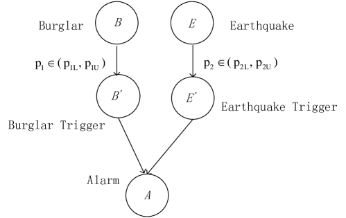
Figure 3: The Belief Noisy-OR structure for Alarm System.

From Table  2 we can see, by the use of ImNOR,

$$m(A=\{F\}|B=\{T\},E=\{T\})=m(A=\{F\}|B=\{T\},E=\{T,F\}),$$ (54)

but by BNOR,

$$m(A=\{F\}|B=\{T\},E=\{T\})<m(A=\{F\}|B=\{T\},E=\{T,F\}).$$ (55)

Eq. (55) fits with our common sense. As soon as we know the earthquake has happened for sure, the less belief should be holding for the proposition the alarm has not gone.

Let the link probability of earthquake be $p_{2}\in(0.7,0.9)$, while the link probability of burglar is set to be $p_{1}\in(\alpha,0.8)$. When $\alpha\rightarrow 0.8$, the uncertainty on $p_{1}$ becomes less. Consequently the uncertainty on the state of Alarm should also decrease. However, as shown in Figure 5, the values of $m(A=\{T,F\}|B=\{T,F\},E=\{F\})$ and $m(A=\{T,F\}|B=\{T,F\},E=\{T,F\})$ by ImNOR remain unchanged although the information for $p_{1}$ becomes more precise. The corresponding results using BNOR show that the belief mass assigned to the uncertainty state of $A$ decreases with the increasing precision of the information on $p_{1}$. Specially, if there is no epistemic uncertainty on $p_{2}$, and the uncertainty on $p_{1}$ declines to 0 ($\alpha=0.8$), the belief mass given to $A=\{T,F\}$ also becomes zero (see Figure 5-a).

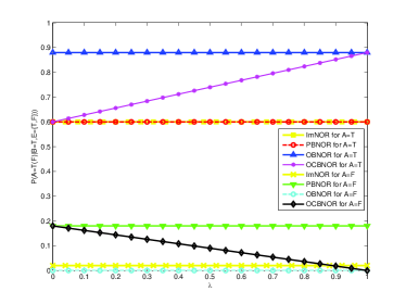
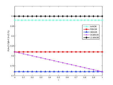
a. $m(A=\{T(F)\}|B=T,E=\{T,F\})$

b. $m(A=\{T,F\}|B=T,E=\{T,F\})$

Figure 4: The different BNOR structures for $m(A|B=T,E=\text{\{T,F\}})$.

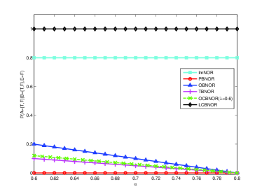
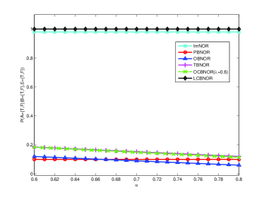
a. $m(A=\{T,F\}|B=\{T,F\},E=F)$

b. $m(A=\{T,F\}|B=\{T,F\},E=\{T,F\})$

Figure 5: The uncertainty of the state of the alarm.

Table 2: The conditional mass distribution for $P(A|B=T,E)$ by ImNOR and different BNORs.

$A$	($B$,$E$) of ImNOR				($B$,$E$) of LC-BNOR
	($T$,$T$)	($T$,$F$)	($T$,$\{T,F\}$)		($T$,$T$)	($T$,$F$)	($T$,$\{T,F\}$)
$T$	0.8800	0.6000	0.6000		0.8800	0.6000	0.6000
$F$	0.0200	0.2000	0.0200		0.0200	0.2000	0.0000
$\{T,F\}$	0.0200	0.2000	0.3800		0.0200	0.2000	0.4000
	($B$,$E$) of PBNOR				($B$,$E$) of OBNOR
	($T$,$T$)	($T$,$F$)	($T$,$\{T,F\}$)		($T$,$T$)	($T$,$F$)	($T$,$\{T,F\}$)
$T$	0.8800	0.6000	0.6000		0.8800	0.6000	0.8800
$F$	0.0200	0.2000	0.1800		0.0200	0.2000	0.0000
$\{T,F\}$	0.0200	0.2000	0.2200		0.0200	0.2000	0.1200
	($B$,$E$) of TBNOR				($B$,$E$) of OCBNOR($\lambda$=0.6)
	($T$,$T$)	($T$,$F$)	($T$,$\{T,F\}$)		($T$,$T$)	($T$,$F$)	($T$,$\{T,F\}$)
$T$	0.8800	0.6000	0.7400		0.8800	0.6000	0.7680
$F$	0.0200	0.2000	0.0900		0.0200	0.2000	0.0720
$\{T,F\}$	0.0200	0.2000	0.1700		0.0200	0.2000	0.1600

Table 3: The conditional mass distribution for $P(A|B=F,E)$ by ImNOR and different BNORs.

A	(B,E) of ImNOR				(B,E) of LC-BNOR
	($F$,$T$)	($F$,$F$)	($F$,{$T$,$F$})		($F$,$T$)	($F$,$F$)	($F$,{$T$,$F$})
$T$	0.7000	0.0000	0.0000		0.7000	0.0000	0.0000
$F$	0.1000	1.0000	0.1000		0.1000	1.0000	0.0000
{$T$,$F$}	0.1000	0.0000	0.9000		0.1000	0.0000	1.0000
	(B,E) of PBNOR				(B,E) of OBNOR
	($F$,$T$)	($F$,$F$)	($F$,{$T$,$F$})		($F$,$T$)	($F$,$F$)	($F$,{$T$,$F$})
$T$	0.7000	0.0000	0.0000		0.7000	0.0000	0.7000
$F$	0.1000	1.0000	0.9000		0.1000	1.0000	0.0000
{$T$,$F$}	0.1000	0.0000	0.1000		0.1000	0.0000	0.3000
	(B,E) of TBNOR				(B,E) of OCBNOR($\lambda$=0.6)
	($F$,$T$)	($F$,$F$)	($F$,{$T$,$F$})		($F$,$T$)	($F$,$F$)	($F$,{$T$,$F$})
$T$	0.7000	0.0000	0.3500		0.7000	0.0000	0.4200
$F$	0.1000	1.0000	0.4500		0.1000	1.0000	0.3600
{$T$,$F$}	0.1000	0.0000	0.2000		0.1000	0.0000	0.2200

Table 4: The conditional mass distribution for $P(A|B=\{T,F\}\triangleq\Theta,E)$ by ImNOR and different BNORs.

$A$	($B$,$E$) of ImNOR				($B$,$E$) of LC-BNOR
	($\Theta$,$T$)	($\Theta$,$F$)	($\Theta$,$\Theta$)		($\Theta$,$T$)	($\Theta$,$F$)	($\Theta$,$\Theta$)
$T$	0.7000	0.0000	0.0000		0.7000	0.0000	0.0000
$F$	0.0200	0.2000	0.0200		0.0000	0.0000	0.0000
{$T$,$F$}	0.0200	0.8000	0.9800		0.0000	1.0000	1.0000
	($B$,$E$) of PBNOR				($B$,$E$) of OBNOR
	($\Theta$,$T$)	($\Theta$,$F$)	($\Theta$,$\Theta$)		($\Theta$,$T$)	($\Theta$,$F$)	($\Theta$,$\Theta$)
$T$	0.7000	0.0000	0.0000		0.8800	0.6000	0.8800
$F$	0.1000	1.0000	0.9000		0.0200	0.2000	0.0000
{$T$,$F$}	0.1000	0.0000	0.1000		0.0200	0.2000	0.1200
	($B$,$E$) of TBNOR				($B$,$E$) of OCBNOR($\lambda$=0.6)
	($\Theta$,$T$)	($\Theta$,$F$)	($\Theta$,$\Theta$)		($\Theta$,$T$)	($\Theta$,$F$)	($\Theta$,$\Theta$)
$T$	0.7900	0.3000	0.5450		0.8080	0.3600	0.6288
$F$	0.0600	0.6000	0.2700		0.0520	0.5200	0.1872
{$T$,$F$}	0.0600	0.1000	0.1850		0.0520	0.1200	0.1840

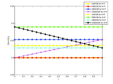
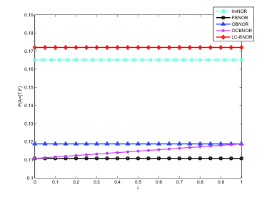
a. $m(A=\{T(F)\})$

b. $m(A=\{T,F\})$

Figure 6: The different BNOR structures for $m(A)$.

Marginal mass $m(A)$ can be obtained by ImNOR and different BNORs, and the results are shown in Table 5 and Figure 6. It is shown that OBNOR provides optimistic results while PBNOR produces a pessimistic one. In order to make a compromise, we can adjust the optimistic coefficient ($\lambda$). Also the contradiction attitudes of ImNOR can be found here. Thus the BNOR methods are more reasonable and informative.

Table 5: The belief mass distribution of the child node $A$.

$A$	ImNOR	LC-BNOR	PBNOR	OBNOR	TBNOR	OCBNOR($\lambda=0.6$)
$T$	0.3996	0.3996	0.3996	0.4528	0.4262	0.4315
$F$	0.4352	0.4284	0.4896	0.4284	0.4590	0.4529
{$T$,$F$}	0.1652	0.1720	0.1108	0.1188	0.1148	0.1156

Using Eqs. (51) and (53), the (conditional) belief mass functions can be transferred to (conditional) pignistic probabilities. The results of

$$BetP(A|B=\{T\},E=\text{\{T,F\}})$$

and $BetP(A)$ are displayed in Figure 7. It can be seen that BNOR can provide us abundant information for decisions with different special requirements. By comparison, ImNOR is more temperate. This is due to the fact that ImNOR assigns more mass values to the vague state $\{T,F\}$. However, if we want to hold the principle that more belief should be given to the uncertain state, LC-BNOR is a better choice (see Figures 4-b and 6-b).

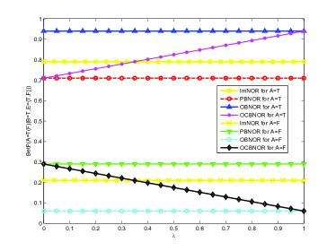
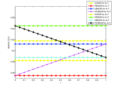
a. $BetP(A|B=T,E=\{T,F\})$

b. $BetP(A)$

Figure 7: The (conditional) pignistic probabilities.

4 Network reliability analysis

In this section we will discuss the application of BNOR on the problem of network reliability analysis. The definition of network reliability and the traditional Bayesian solution are first recalled. Then the reliability evaluation strategy using BNOR model will be described in detail.

4.1 Network reliability and Bayesian network solution

The network reliability considered here is two-terminal reliability, defined as the probability that there is an operative path between source nodes $n_{1}$ and sink nodes $n_{N}$ in the network. Nodes are assumed to be operational at all times, and edge failures are assume to be statistically independent.

Let graph $G(N,E)$ represent a network, where $N$ denotes the set of nodes and $E$ is the set of links. For the network shown in Figure 8-a, $N=\left\{n_{1},n_{2},n_{3},n_{4}\right\}$, $E=\left\{e_{1,}e_{2},e_{3},e_{4}\right\}$. Define $|N|$ new variables, $N_{i},i=1,2,\cdots,|N|$ , indicating whether the communication between $n_{1}$ and $n_{i}$ is successful. Let $N^{+}(n_{i})=\left\{n_{j}|<n_{j},n_{i}>\in E\right\}$, for every element of which sets, $n_{j}$, there is a path from $n_{j}$ to $n_{i}$. And let $E^{+}(n_{i})=\left\{e_{k}=<n_{j},n_{i}>|n_{j}\in N^{+}(n_{i})\right\}$ denote the sets of edges directed to node $n_{i}$.

Zhen et al. ³⁹ presented a method for reliability evaluating of networks based on BN. The nodes and edges of BN can be created according to $G(N,E)$:

1. The root nodes of BN are $N_{1}$ and the edges in $E$.

2. The non-root nodes of BN are $N_{i},i\neq 1$. And

   $$Pa(N_{i})=\left\{N_{j}|n_{j}\in N^{+}(n_{i})\right\}\cup\left\{e_{k}|e_{k}\in E^{+}(n_{i})\right\}.$$ (56)

Bayesian networks’ inference algorithms can be evoked then to calculate the network reliability $P(N_{s})$. The BN framework for the network described in Figure 8-a can be seen in Figure 8-b.

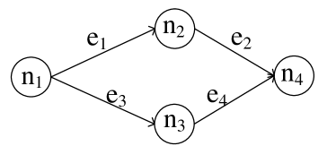
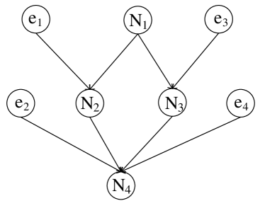
a. Directed network

b. BN solution

Figure 8: An example of directed network and its BN solution.

4.2 Reliability evaluation using BNOR

For the network shown in Figure 9, its reliability can be defined by the probability that there is a working path connected from $n_{1}$ to $n_{5}$. The network is operating if the two terminal nodes $n_{1}$ and $n_{5}$ are connected by operational edges. Let $S$ denote the state of the network. It has binary states with $T$ (working) or $F$ (fail). The values for failure rates of each edge are

$$\lambda_{e_{1}}=\lambda_{e_{3}}=\lambda_{e_{5}}=1.5*10^{-3}~{}\mathrm{h^{-1}},\lambda_{e_{2}}=\lambda_{e_{4}}=\lambda_{e_{6}}=1.8*10^{-3}~{}\mathrm{h}^{-1}.$$

Figure 9: The network with 5 nodes.

Consider the mission time $t=200~{}\mathrm{h}$. The probability distribution of each edge is given in Table  6.

Table 6: The probability distribution of each edge of the network

	$e_{1}$	$e_{2}$	$e_{3}$	$e_{4}$	$e_{5}$	$e_{6}$
$T$	0.8025	0.6977	0.8025	0.6977	0.8025	0.6977
$F$	0.1975	0.3023	0.1975	0.3023	0.1975	0.3023

The traditional Bayesian network approach is first adopted to calculate the reliability. Using the method described in Section 4.1, we can create a Bayesian network solution model (see Figure 10). By applying the Junction Tree (JT) inference algorithm, we can obtain the exact value of the network reliability $p(S=T)=0.9148$.

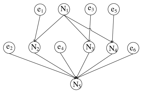
Figure 10: The BN network solution.

In the next two subsections, different BNOR structures (PBNOR, OBNOR, TBNOR, OCBNOR and LC-BNOR) will be applied to estimate the network reliability. The BNOR model for this network is shown in Figure 11. The fail of edge $e_{i}$ can be regarded as an inhibition. For example, in the network displayed in Figure 9, even if $N_{2}$ is in the working state $T$, $N_{5}$ may not in state $T$ due to the fail of $e_{2}$. The inhibition can be measured by link probabilities $p_{e_{i}},i=1,2,\cdots,5$.

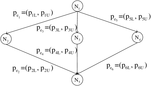
Figure 11: The BNOR model for network reliability.

4.3 BNOR model, case with no epistemic uncertainty

If there is no epistemic uncertainty, neither on the variable state or on link probabilities, i.e.,

$$m(N_{1}=\left\{T,F\right\})=0,$$

and

$$p_{iL}=p_{iU}=p(e_{i}=T),i=1,2,\cdots,6,$$

the same results can be obtained by the use of all BNORs and ImNOR:

$$m(S=\{T\})=0.9148,~{}m(S=\{F\})=0.0852,~{}m(S=\{T,F\})=0.$$

It can be seen that, if there is no epistemic uncertainty introduced, the reliability estimation results previously obtained by traditional BN method can be recovered. This fact indicates that BNOR is a general extension of Noisy-OR structure in the framework of belief functions, and it is entirely compatible with the probabilistic solution. The $Bel$ and $Pl$ measures can be obtained by Eqs. (10) and (11) respectively. The following results can be obtained:

$$Bel(S=\{T\})=0.9148,~{}p(S=T)=0.9148,~{}Pl(S=\{T\})=0.9148.$$ (57)

4.4 BNOR model, case with an epistemic uncertainty

In this test, the case with some epistemic uncertainty on link probabilities is considered. The lower and upper probability bounds of link probabilities $p_{e_{i}}$ are listed in Table 7. The results by five BNORs and ImNOR are illustrated in Table 8.

Table 7: The probability intervals of the inhibition parameters

	$p_{e_{1}}$	$p_{e_{2}}$	$p_{e_{3}}$	$p_{e_{4}}$	$p_{e_{5}}$	$p_{e_{6}}$
$P_{iL}$	0.7525	0.6477	0.8025	0.6977	0.8025	0.6977
$P_{iU}$	0.8525	0.7477	0.8025	0.6977	0.8025	0.6977

In Figures 12-a and 12-b, the results of the evaluation of the network system varying with the optimism coefficient $\lambda$ are demonstrated. It can be found that when $\lambda$ grows from 0 up to 1, the mass on “the system is working” (i.e., $m(S=\{T\})$) increases. On the contrary, $m(S=\{F\})$ decreases. This meets with our common sense of optimistic and pessimistic decisions. However, ImNOR provides opposite attitudes towards $m(S=\{T\})$ and $m(S=\{F\})$. The performance of ImNOR is similar to PBNOR for calculating $m(S=\{T\})$, while similar to OBNOR for calculating $m(S=\{F\})$.

Figure 12-c illustrates that the mass assigned to the uncertain state $\{T,F\}$ by LC-BNOR is larger than that by the other models. This is due to the principle LC-BNOR upholds is that one should never give more support than justified to any subset of the discernment frame.

Let the interval of link probability $p_{e_{1}}$ be $[0.7525,0.8525]$ and the corresponding interval of $p_{e_{2}}$ be $[0.6977,0.6977]-[\alpha,-\alpha]$. The length of the interval, $2\alpha$, reflects the degree of uncertainty to some extend. Figure 12-d depicts the mass assigned to the uncertain state $m(S=\{T,F\})$ varying with $\alpha$. It can be seen that the uncertainty on system’s state increases with the increasing of $\alpha$. LC-BNOR is the most sensitive to uncertainty variation among the six NOR models.

In this case, the credibility and plausibility measures on $S=\{T\}$ are not the same, and they bound the network reliability. For example, if we use OCBNOR ($\lambda=0.6$), from Table 8 we can see the belief mass assignment of the network state $S$:

$$m(S=\{T\})=0.9082,~{}m(S=\{F\})=0.0741,~{}m(S=\{T,F\})=0.0177.$$ (58)

The following results can be obtained:

$$Bel(S=\{T\})=0.9082,~{}p(S=T)=0.9148,~{}Pl(S=\{T\})=0.9259.$$ (59)

Further decisions can be made based on these uncertainty knowledge.

Table 8: The belief mass distribution of the network system.

S	ImNOR	LC-BNOR	PBNOR	OBNOR	TBNOR	OCBNOR($\lambda=0.6$)
$T$	0.9007	0.8818	0.9007	0.9133	0.9070	0.9082
$F$	0.0702	0.0540	0.0828	0.0683	0.0755	0.0741
{$T$,$F$}	0.0291	0.0642	0.0165	0.0184	0.0175	0.0177

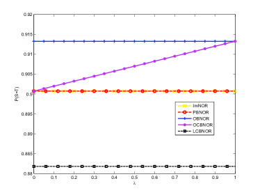
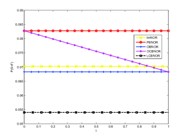
a. $m(S=\{T\})$

b. $m(S=\{F\})$

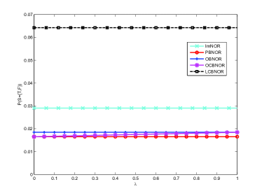
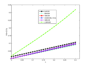
c. $m(S=\{T,F\})$ varying with $\lambda$

d. $m(S=\{T,F\})$ varying with $\alpha$

Figure 12: The different BNOR structures for $m(S)$.

The information on credal level can be transformed to the pignistic level by Eq. (51) where the decisions can be made more easily. The probability distributions by different models are listed in Table  9. As it can be observed in Figure 13, with the increasing of $\lambda$, the pignistic probability for $S=T$ increases, on the other hand decreases for $S=F$. For $S=T$, OBNOR gives a upper bound and PBNOR gives a lower bound. While for $S=F$, OBNOR gives a lower bound and PBNOR gives a upper bound. This is in accordance with the optimistic and pessimistic principles. However, the attitude of ImNOR is ambiguous.

Table 9: The probability distribution of the network system.

S	ImNOR	LC-BNOR	PBNOR	OBNOR	TBNOR	OCBNOR($\lambda=0.6$)
$T$	0.9152	0.9139	0.9090	0.9225	0.9157	0.9171
$F$	0.0848	0.0861	0.0910	0.0775	0.0843	0.0829

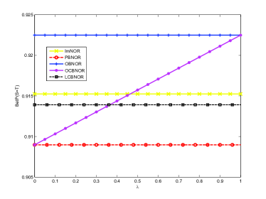
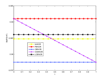
a. $BetP(S=T)$

b. $BetP(S=F)$

Figure 13: The different BNOR structures for $BetP(S)$.

4.5 Discussion

From the experimental results, it can be concluded that when there is no epistemic uncertainty in the network, BNOR degrades to the traditional Bayesian method. However, if there indeed exists imperfect knowledge, BNOR model can provide us more information in the form of lower bounds ($Bel$) and upper bounds ($Pl$). A pessimistic decision can be made according to the $Bel$ value, which provides us the worst value of the network reliability. On the contrary, $Pl$ is the maximum degree of belief that can support the connectivity of the network, from which an optimistic decision can be made. These measures are of great value when we have to make a compromise between risks and costs. Also these knowledge on the credal level can be transformed to the pignistic level through Smets method. Then common principles in decision theory such as the minimal expected cost (risk) criterion can be evoked.

5 Conclusion

In this paper, the BNOR model under the framework of belief functions, as an extension of the traditional NOR model, is developed to express several kinds of uncertainty in the independent causal interactions. It is proved that BNOR can be implemented to propagate uncertain information through employing the Bayesian networks tools. In practice, BNOR is more flexible than existing NOR models because it offers a general Bayesian framework that allows us to adopt the exact inference algorithm in their original form without modification, and then by adjusting necessary parameters to obtain results which satisfy the special requirements of engineers. Finally, the application on the reliability evaluation problem of networked systems demonstrates the effectiveness of BNOR model.

BNOR is applicable to systems with binary variables. An extension of BNOR suitable to multi-value variables should be regarded as a future development. Furthermore, the uncertainty on link probabilities may not be given in the form of intervals in practice. How to take advantage of the independence of causal interactions with different types of uncertain knowledge is another considerable problem to be investigated. This paper mainly focuses on theoretical work. Applications of BNOR on more complex situations will be considered in the future.

References

- Jensen 1996 F. V. Jensen, An introduction to Bayesian networks (UCL press, London, 1996).
- Marquez et al. 2010 D. Marquez, M. Neil, and N. Fenton, “Improved reliability modeling using bayesian networks and dynamic discretization,” Reliab. Eng. Syst. Safe., vol. 95, no. 4, pp. 412–425, 2010.
- Doguc and Ramirez-Marquez 2009 O. Doguc and J. E. Ramirez-Marquez, “A generic method for estimating system reliability using bayesian networks,” Reliab. Eng. Syst. Safe., vol. 94, no. 2, pp. 542–550, 2009.
- Portinale et al. 2010 L. Portinale, D. C. Raiteri, and S. Montani, “Supporting reliability engineers in exploiting the power of dynamic bayesian networks,” Int. J. Approx. Reason., vol. 51, no. 2, pp. 179–195, 2010.
- Neil and Marquez 2012 M. Neil and D. Marquez, “Availability modelling of repairable systems using bayesian networks,” Eng. Appl. Artif. Intell., vol. 25, no. 4, pp. 698–704, 2012.
- Antonucci 2011 A. Antonucci, “The imprecise noisy-or gate,” Proc. 14th International Conference on Information Fusion . IEEE, 2011, pp. 1–7.
- Pearl 1988 J. Pearl, Probabilistic Reasoning in Intelligent Systems: Networks of Plausble Inference (Morgan Kaufmann Pub, 1988).
- Srinivas 1993 S. Srinivas, “A generalization of the noisy-or model,” Proc. 9th International Conference on Uncertainty in Artificial Intelligence. Morgan Kaufmann Publishers Inc., 1993, pp. 208–215.
- Fallet et al. 2012 G. Fallet, P. Weber, C. Simon, B. Iung, and C. Duval, “Evidential network-based extension of leaky noisy-or structure for supporting risks analyses,” Proc. 8th International Symposium SAFEPROCESS, 2012, p. 00.
- Shafer 1976 G. Shafer, A mathematical theory of evidence (Princeton University Press, 1976).
- Denoeux 1995 T. Denoeux, “A -nearest neighbor classification rule based on dempster-shafer theory,” IEEE Trans. Syst. Man. Cybern., vol. 25, no. 5, pp. 804–813, 1995.
- Liu et al. 2014 Z.-g. Liu, Q. Pan, J. Dezert, and G. Mercier, “Credal classification rule for uncertain data based on belief functions,” Pattern. Recogn., vol. 47, no. 7, pp. 2532–2541, 2014.
- Liu et al. 2015 Z.-g. Liu, Q. Pan, G. Mercier, and J. Dezert, “A new incomplete pattern classification method based on evidential reasoning,” IEEE Trans. Cybern., vol. 45, no. 4, pp. 635–646, 2015.
- Masson and Denoeux 2008 M.-H. Masson and T. Denoeux, “ECM: An evidential version of the fuzzy -means algorithm,” Pattern. Recogn., vol. 41, no. 4, pp. 1384–1397, 2008.
- Denœux and Masson 2004 T. Denœux and M.-H. Masson, “EVCLUS: evidential clustering of proximity data,” IEEE Trans. Syst. Man Cybern. Part B Cybern., vol. 34, no. 1, pp. 95–109, 2004.
- Zhou et al. 2015a K. Zhou, A. Martin, Q. Pan, and Z.-G. Liu, “Evidential relational clustering using medoids,” Proc. 18th International Conference on Information Fusion (Fusion). IEEE, 2015, pp. 413–420.
- Zhou et al. 2015b K. Zhou, A. Martin, Q. Pan, and Z.-g. Liu, “ECMdd: Evidential c-medoids clustering with multiple prototypes,” Pattern. Recogn., doi: 10.1016/j.patcog.2016.05.005, 2016.
- Wei et al. 2013 D. Wei, X. Deng, X. Zhang, Y. Deng, and S. Mahadevan, “Identifying influential nodes in weighted networks based on evidence theory,” Physica A., vol. 392, no. 10, pp. 2564–2575, 2013.
- Zhou et al. 2014a K. Zhou, A. Martin, and Q. Pan, “Evidential communities for complex networks,” Proc. 15th International Conference on Information Processing and Management of Uncertainty in Knowledge-Based Systems. Springer, 2014, pp. 557–566.
- Zhou et al. 2015b K. Zhou, A. Martin, Q. Pan, and Z.-g. Liu, “Median evidential -means algorithm and its application to community detection,” Knowl.-based Syst., vol. 74, pp. 69–88, 2015.
- Zhou et al. 2015c K. Zhou, A. Martin, and Q. Pan, “A similarity-based community detection method with multiple prototype representation,” Physica A., vol. 438, pp. 519–531, 2015.
- Denoeux 2013 T. Denoeux, “Maximum likelihood estimation from uncertain data in the belief function framework,” IEEE Trans. Knowl. Data. En., vol. 25, no. 1, pp. 119–130, 2013.
- Côme et al. 2009 E. Côme, L. Oukhellou, T. Denoeux, and P. Aknin, “Learning from partially supervised data using mixture models and belief functions,” Pattern. Recogn., vol. 42, no. 3, pp. 334–348, 2009.
- Zhou et al. 2014b K. Zhou, A. Martin, and Q. Pan, “Evidential-EM algorithm applied to progressively censored observations,” Proc. 15th International Conference on Information Processing and Management of Uncertainty in Knowledge-Based Systems. Springer, 2014, pp. 180–189.
- Simon et al. 2008 C. Simon, P. Weber, and A. Evsukoff, “Bayesian networks inference algorithm to implement dempster shafer theory in reliability analysis,” Reliab. Eng. Syst. Safe., vol. 93, no. 7, pp. 950–963, 2008.
- Simon and Weber 2009 C. Simon and P. Weber, “Evidential networks for reliability analysis and performance evaluation of systems with imprecise knowledge,” IEEE Trans. Reliab., vol. 58, no. 1, pp. 69–87, 2009.
- Yaghlane and Mellouli 2008 B. B. Yaghlane and K. Mellouli, “Inference in directed evidential networks based on the transferable belief model,” Int. J. Approx. Reason., vol. 48, no. 2, pp. 399–418, 2008.
- Smets and Kennes 1994 P. Smets and R. Kennes, “The transferable belief model,” Artif. Intell., vol. 66, no. 2, pp. 191 – 234, 1994.
- Heckerman and Breese 1996 D. Heckerman and J. S. Breese, “Causal independence for probability assessment and inference using bayesian networks,” IEEE Trans. Syst. Man Cy. A., vol. 26, no. 6, pp. 826–831, 1996.
- Cozman 2004 F. G. Cozman, “Axiomatizing noisy-or,” Proc. 16th European Conference on Artificial Intelligence, 2004, pp. 979–980.
- Lian-wei and Hai-peng 2006 Z. Lian-wei and G. Hai-peng, Introduction to bayesian networks (Science Press, 2006).
- Smets 2002 P. Smets, “The application of the matrix calculus to belief functions,” Int. J. Approx. Reason., vol. 31, no. 1, pp. 1–30, 2002.
- Ferson et al. 2004 S. Ferson, R. B. Nelsen, J. Hajagos, D. J. Berleant, J. Zhang, W. T. Tucker, L. R. Ginzburg, and W. L. Oberkampf, “Dependence in probabilistic modeling, Dempster-Shafer theory, and probability bounds analysis,” Citeseer, 2004, vol. 3072.
- Walley 1991 P. Walley, Statistical reasoning with imprecise probabilities (Chapman and Hall, London, 1991).
- Utkin and Coolen 2007 L. V. Utkin and F. P. Coolen, “Imprecise reliability: an introductory overview,” Computational intelligence in reliability engineering (Springer, 2007).
- Smets 2005a P. Smets, “Decision making in the TBM: the necessity of the pignistic transformation,” Int. J. Approx. Reason., vol. 38, no. 2, pp. 133–147, 2005.
- Smets 2005b P. Smets, “Belief functions on real numbers,” Int. J. Approx. Reason., vol. 40, no. 3, pp. 181–223, 2005.
- Mercier et al. 2005 D. Mercier, G. Cron, T. Denœux, and M. Masson, “Fusion of multi-level decision systems using the transferable belief model,” Proc. 8th International Conference on Information Fusion, IEEE, 2005, pp. 885–892.
- Zhen et al. 2011 L. Zhen, S. Xin-li, G. xun Ji, and Z. yong Liu, “Reliability evaluating of networks with imperfect nodes based on bayes network,” Syst. Eng. Theory Pract., vol. 31, no. 10, pp. 1974–1984, 2011.