Optomechanical Self-Oscillations in an Anharmonic Potential:
Engineering a Nonclassical Steady State

Abstract

We study self-oscillations of an optomechanical system, where coherent mechanical oscillations are induced by a driven optical or microwave cavity, for the case of an anharmonic mechanical oscillator potential. A semiclassical analytical model is developed to characterize the limit cycle for large mechanical amplitudes corresponding to a weak nonlinearity. As a result, we predict conditions to achieve subpoissonian phonon statistics in the steady state, indicating classically forbidden behavior. We compare with numerical simulations and find very good agreement. Our model is quite general and can be applied to other physical systems such as trapped ions or superconducting circuits.

I Introduction

The state of individual physical systems is determined by the interaction to their environment. Most natural environments randomly couple the system to many degrees of freedom and bring about classical states Joos et al. (2003); Zurek (2003). But artificial environments can be specifically engineered Poyatos et al. (1996), typically by strongly coupling the system to a small set of well-controlled degrees of freedom, for the purpose of reaching a particular steady state that may have nonclassical features. Such states are a crucial resource for quantum information processing Nielsen and Chuang (2010); Mari and Eisert (2012), furthermore they are of fundamental interest for testing quantum mechanics in previously unexplored regimes Bassi et al. (2013).

Quantum reservoir engineering has been used to demonstrate nonclassical steady states on various platforms such as atomic clouds Krauter et al. (2011), superconducting qubits Murch et al. (2012); Shankar et al. (2013), and trapped ions Kienzler et al. (2015). In the context of optomechanics, driving the optical cavity on both sidebands can lead to highly nonclassical states. Steady-state mechanical squeezed states have been proposed Kronwald et al. (2013) and realized Wollman et al. (2015); Pirkkalainen et al. (2015); Lecocq et al. (2015) by driving dominantly on the red sideband. For dominant blue sideband driving, stabilization of mechanical Fock states has been proposed Rips et al. (2012), requiring in addition a strongly intrinsic mechanical anharmonicity, which has not been realized in mechanical oscillators.

For weaker anharmonicity, such a setup with dominant driving on the blue sideband leads to coherent excitation of mechanical self-oscillations and therefore laser-like mechanical states, which we investigate in this article. For the case in which the intrinsic anharmonicity is the system’s dominant nonlinearity, we derive a semiclassical analytical description to describe the system dynamics in terms of the amplitude. The description is valid for large mechanical amplitudes, where we compare to numerical simulations and find excellent agreement.

For such a setup we derive conditions on the system parameters for the steady states to show number squeezing, which is characterized by subpoissonian number statistics. This nonclassical feature is well-studied in the photon statistics of lasers and can be achieved e.g. by pumping the cavity with an ordered sequence of separated flying atoms Golubev and Sokolov (1984) or coupling to one-and-the-same fixed atom McKeever et al. (2003). The subpoissonian statistics in these system is in contrast to ordinary lasers, where the random pumping via a large number of atoms results in fully classical coherent or even superpoissonian states.

In the context of optomechanical self-oscillations Marquardt et al. (2006), recently several proposals have been made to achieve the analogous phenomenon for phonons, i.e. subpoissonian statistics for a phonon laser Rodrigues and Armour (2010); Qian et al. (2012); Armour and Rodrigues (2012); Nation (2013); Lörch et al. (2014); Lörch and Hammerer (2015). All of these proposals rely on the nonlinearity of the optomechanical interaction. In contrast, we consider a linearized optomechanical interaction and use the intrinsic nonlinearity of the mechanical oscillator to achieve subpoissonian statistics.

While we will employ optomechanical terminology throughout this article, the underlying model is quite general and can be applied to other implementations. For example, phonon lasing has been demonstrated with trapped ions Vahala et al. (2009); Knünz et al. (2010) and ion potentials can be engineered to have a large nonlinearity, so that the dynamics will be similar to the discussion in this paper. A further implementation could be done with superconducting circuits, which can have large effective Kerr nonlinearities.

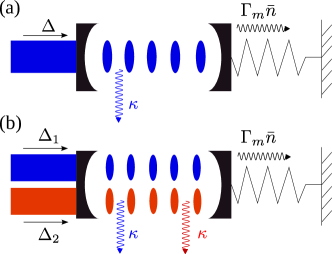
Figure 1: Illustration of the studied systems. (a) A standard optomechanical system, where an optical cavity mode with decay rate $\kappa$ is dispersively coupled to a mechanical mode of resonance frequency $\omega_{m}$, decay rate $\Gamma_{m}$ and bath occupation $\bar{n}$. The cavity is driven by a laser on the blue sideband $\Delta\approx\omega_{m}$ to excite coherent mechanical oscillations. (b) Another laser tone with detuning $\Delta_{2}=-\omega_{m}$ is added on the red side to reduce the effective temperature of the mechanical bath.

This article is structured as follows: In the following Section II we develop an analytical description for the system. For simplicity this is done for the case illustrated in Fig. 1 (a), where only one laser drives the cavity. In Section 3 we then generalize to the two-laser case depicted in Fig. 1 (b). Finally in Section IV we discuss these results and compare to numerical solutions of the quantum master equation.

II Analytical description

In this section we derive the main results for a system that is driven by only one laser and generalize later in Section 3 to the case of two lasers.

II.1 Model

We consider a bosonic mode $b$ of a mechanical oscillator with intrinsic Kerr anharmonicity that may be described by the Hamiltonian $H_{m}=\omega_{m}b^{\dagger}b+K(b^{\dagger}b)^{2}$ coupled to a driven optical cavity mode $a$ with Hamiltonian $H_{c}=\omega_{c}a^{\dagger}a+\Omega\left(ae^{i\omega_{L}t}+a^{\dagger}e^{-i\omega_{L}t}\right)$. Here $K$ is the Kerr anharmonicity parameter and $\omega_{m}$, $\omega_{c}$ and $\omega_{L}$ are the frequencies of the mechanical and the optical mode, as well as the optical drive of strength $\Omega$. The operators $a^{\dagger},a$ and $b^{\dagger},b$ denote the creation and annihilation operators for the optical cavity and the mechanical oscillator. The Kerr anharmonicity approximates an anharmonic Duffing term $\propto D(b+b^{\dagger})^{4}$ in the potential, the validity of this rotating wave approximation is discussed in Section IV.2.

The optomechanical interaction is described by $H_{\mathrm{int}}=-g_{0}a^{\dagger}a(b+b^{\dagger})$ with single-photon coupling $g_{0}$. Defining the detuning $\Delta=\omega_{L}-\omega_{c}$, we switch to a rotating frame for the laser to obtain a time-independent Hamiltonian $H_{c}=-\Delta a^{\dagger}a+\Omega(a+a^{\dagger})$, while $H_{m}$ and $H_{\mathrm{int}}$ are unchanged. In the limit of small $g_{0}$ and large number of photons $n_{c}$ in the cavity, we further simplify the Hamiltonian and linearize Aspelmeyer et al. (2014) the interaction to $H_{I}=-g(a+a^{\dagger})(b+b^{\dagger})$, where $g=g_{0}\sqrt{n_{c}}$ is the linearized coupling, so that in total $H=H_{m}+H_{c}+H_{I}$ is

$$H=\omega_{m}b^{\dagger}b+K(b^{\dagger}b)^{2}-\Delta a^{\dagger}a+\Omega\left(a+a^{\dagger}\right)-g(a+a^{\dagger})(b+b^{\dagger})\>.$$ (1)

Note that we already neglected a constant force $\propto g_{0}\langle a^{\dagger}a\rangle$ which results in a small shift of the mean position of the oscillator.

The incoherent coupling of the system to its environment can be modeled Aspelmeyer et al. (2014) with the Lindblad operators

$$\mathcal{L}_{m}\rho= -\Gamma_{m}(n_{\mathrm{th}}+1)(b^{\dagger}b\rho+\rho b^{\dagger}b-2b\rho b^{\dagger})$$

$$-\Gamma_{m}n_{\mathrm{th}}(bb^{\dagger}\rho+\rho bb^{\dagger}-2b^{\dagger}\rho b)\>,$$

$$\mathcal{L}_{c}\rho= -\kappa(a^{\dagger}a\rho+\rho a^{\dagger}a-2a\rho a^{\dagger})\>,$$ (2)

where $\kappa$ and $\Gamma$ are the amplitude decay rates of the cavity and the mechanical oscillator. We assumed here a zero-temperature bath for the optical cavity and a thermal occupation $n_{\mathrm{th}}$ of the mechanical bath. Including these Lindblad operators, the full quantum master equation for this system reads

$$\dot{\rho}=-i[H,\rho]+\mathcal{L}_{m}\rho+\mathcal{L}_{c}\rho\>.$$ (3)

To obtain a semiclassical description we transform the quantum master equation (3) into a partial differential equation for the Wigner distribution $W(\beta,\beta^{*})$ using the translation rules Gardiner and Zoller (2004) $b\rho\rightarrow(\beta+q\partial_{\beta^{*}})W$, $b^{\dagger}\rho\rightarrow(\beta^{*}-p\partial_{\beta})W$ and their complex conjugates to obtain

$$\begin{split}\partial_{t}W=&\big{[}-i{\Delta}\partial_{\alpha}\alpha+i\omega_{m}\partial_{\beta}\beta-ig\big{(}\partial_{\alpha}(\beta+\beta^{*})+\partial_{\beta}(\alpha+\alpha^{*})\big{)}\\ &+\Gamma_{m}(\partial_{\beta}\beta+\tfrac{1}{2}(2\bar{n}+1)\partial_{\beta}\partial_{\beta^{*}})+\kappa(\partial_{\alpha}\alpha+\tfrac{1}{2}\partial_{\alpha}\partial_{\alpha^{*}})\\ &+iK\partial_{\beta}(2|\beta|^{2}\beta-\beta-\tfrac{1}{8}\partial_{\beta}^{2}\partial_{\beta^{*}}\beta)\big{]}W+\mathrm{h.c.}\>.\end{split}$$ (4)

Assuming large mechanical amplitudes we neglect third-order derivatives in a truncated Kramers-Moyal expansion Carmichael (1999) so that Eq. (4) becomes a Fokker-Planck equation. Its corresponding Langevin equations are

$$\dot{\alpha}=(i{\Delta}-\kappa)\alpha+ig(\beta+\beta^{*})+\eta_{\alpha},$$ (5)

$$\dot{\beta}=\big{(}-i\omega_{m}-iK(2|\beta|^{2}-1)-\Gamma_{m}\big{)}\beta+ig(\alpha+\alpha^{*})+\eta_{\beta}\>,$$ (6)

where $\eta_{\alpha},\eta_{\beta}$ are zero-mean complex white noise processes with the correlators $\braket{\eta_{\alpha}(t)\eta_{\alpha^{*}}(t^{\prime})}=\kappa\delta(t-t^{\prime})$, $\braket{\eta_{\beta}(t)\eta_{\beta^{*}}(t^{\prime})}=\Gamma_{m}(2\bar{n}+1)\delta(t-t^{\prime})$, and $\braket{\eta_{i}(t)\eta_{i}(t^{\prime})}=\braket{\eta_{i}(t)\eta_{j^{*}}(t^{\prime})}=0$ for $i,j\in\{\alpha,\beta\}$ and $i\neq j$.

II.2 Adiabatic Elimination of the Cavity

To eliminate the optical amplitude $\alpha$, we assume the cavity decay rate to be much greater than the interaction strength and the mechanical damping, i.e. $\kappa\gg g,\Gamma_{m}$, and furthermore we assume that the mechanical frequency is much larger than the interaction strength $\omega_{m}\gg g$. These are realistic assumptions that can be achieved in typical optomechanical experiments. For the mechanical amplitude we choose the ansatz $\beta=Be^{-i\phi}e^{-i\omega_{m}(B)t}$, with

$$\omega_{m}(B)=\omega_{m}+2KB^{2}-K\>,$$ (7)

where $\phi(t)$ and $B(t)$ are real-valued numbers describing the phase and amplitude of the oscillator. According to our assumptions they are slowly varying on the time scale of $\kappa^{-1}$. In contrast to the otherwise quite analogous treatment of optomechanical limit cycles given in Marquardt et al. (2006); Rodrigues and Armour (2010); Armour and Rodrigues (2012), we have to choose here an amplitude-dependent frequency $\omega_{m}(B)$ because of the factor $-iK(2|\beta|^{2}-1)$ in the equation of motion (6). Defining the Fourier transform as $\mathcal{F}[f(t)]=\int\mathrm{d}te^{-i\omega t}f(t),\quad\mathcal{F}^{-1}[g(\omega)]=\frac{1}{2\pi}\int\mathrm{d}\omega e^{i\omega t}g(\omega),$ we can solve Eq. (5) for $\alpha=\braket{\alpha}+\delta\alpha$ by adiabatic elimination to obtain

$$\braket{\alpha}(t)=ig\left(\frac{\beta(t)}{-i\omega_{m}(B)-i\Delta+\kappa}+\frac{\beta^{*}(t)}{i\omega_{m}(B)-i\Delta+\kappa}\right),$$ (8)

$$\delta\alpha(t)=\mathcal{F}^{-1}\left[\frac{\eta_{\alpha}(\omega)}{i\omega-i\Delta+\kappa}\right].$$ (9)

Inserting Eq. (8) into Eq. (6) but neglecting the terms $\sim\beta^{*}$ in a rotating-wave approximation Walls and Milburn (2008), since they will rotate at a frequency $2\omega_{m}(B)$ with respect to $\beta$, we find the equation of motion

$$\begin{split}\dot{\beta}=&-(i\omega_{m}(B)+i\delta\omega+\Gamma_{m}+\Gamma_{\mathrm{opt}})\beta+\eta_{\beta}+ig\left(\delta\alpha+\delta\alpha^{*}\right)\>.\end{split}$$ (10)

Here, we defined the optically induced damping and frequency shift

$$\Gamma_{\mathrm{opt}}(\Delta,B)=g^{2}\left(\frac{\kappa}{({\Delta}+\omega_{m}(B))^{2}+\kappa^{2}}-\frac{\kappa}{({\Delta}-\omega_{m}(B))^{2}+\kappa^{2}}\right),$$ (11)

$$\delta\omega(\Delta,B)=g^{2}\left(\frac{\omega_{m}(B)+\Delta}{(\Delta+\omega_{m}(B))^{2}+\kappa^{2}}+\frac{\Delta-\omega_{m}(B)}{(\Delta-\omega_{m}(B))^{2}+\kappa^{2}}\right).$$ (12)

These results are analogous to the standard linearized optomechanical Hamiltonian Aspelmeyer et al. (2014), but with amplitude-dependent frequency. Next we switch to polar coordinates and focus on the equation of motion for the amplitude

$$\dot{B}=-(\Gamma_{m}+\Gamma_{\mathrm{opt}})B+\eta_{T}^{-},$$ (13)

$$\eta_{T}^{-}=\tfrac{1}{2}\eta_{\beta}e^{i\varphi}e^{i\omega_{m}(B)t}-{g}\sin\left({\varphi}+{\omega_{m}(B)t}\right)\delta\alpha+\mathrm{h.c.},$$ (14)

where $B=|\beta|$ and $\eta_{T}^{-}$ refers to the noise in radial direction.

Following Balanov et al. (2008) we evaluate the diffusion constant $D_{B}=2\int\mathrm{d}\tau\braket{\eta_{T}^{-}(t),\eta_{T}^{-}(t+\tau)}$ to convert Eq. (13) into an effective Langevin equation $\dot{B}=-(\Gamma_{m}+\Gamma_{\mathrm{opt}})B+\sqrt{D_{B}}\eta_{B},$ where $\eta_{B}$ is a Gaussian white-noise process. Since this equation is independent of the phase $\varphi$ we can also write down a Fokker-Planck equation for the amplitude probability distribution $W_{B}$

$$\partial_{t}W(B)=-\partial_{B}A_{B}W(B)+\frac{1}{2}\partial_{B}^{2}D_{B}W(B)$$ (15)

with drift $A_{B}=-(\Gamma_{m}+\Gamma_{\mathrm{opt}})B$ for the radial coordinate. In total we have $D_{B}=\frac{1}{2}(D_{m}+D_{\mathrm{opt}})$, where $D_{m}=\Gamma_{m}(2\bar{n}+1)$ refers to the intrinsic mechanical part. After integration we find the optically induced part of the amplitude diffusion

$$D_{\mathrm{opt}}(\Delta,B)=g^{2}\left(\frac{\kappa}{(\Delta+\omega_{m}(B))^{2}+\kappa^{2}}+\frac{\kappa}{(\Delta-\omega_{m}(B))^{2}+\kappa^{2}}\right),$$ (16)

again deviating from the well-known results in linearized optomechanics only by the amplitude dependence of $\omega_{m}(B)$. Both optically induced damping (11) and diffusion (16) are given by the same Lorentzian as illustrated in Fig. 2.

II.3 Steady-State Solution and Fano Factor

We have derived an effective equation of motion in the form of a Fokker-Planck equation for the amplitude $B$. We will now calculate its steady-state solution. The analytical solution of the Fokker-Planck equation (15) is given by Carmichael (1999)

$$W_{B}=\mathcal{N}\frac{1}{D_{B}}\mathrm{exp}\left(2\int\limits_{0}^{B}\frac{A_{B^{\prime}}}{D_{{B^{\prime}}}}\mathrm{d}B^{\prime}\right),$$ (17)

where $\mathcal{N}$ is a normalization constant. Rather than calculating the full solution, it is more instructive to analyze the solution after the following approximations. The center $B_{0}$ of the amplitude distribution obeys the fourth-order equation

$$A_{B}(B_{0})=-\left[\Gamma_{m}+\Gamma_{\mathrm{opt}}(B_{0})\right]B_{0}=0\>,$$ (18)

see the definition of the optical damping in Eq. (11). This can be simplified by assuming $(\omega_{m}(B_{0})-\Delta)^{2}\ll(\omega_{m}(B_{0})+\Delta)^{2}$ and approximating $\Gamma_{\mathrm{opt}}\approx-\frac{g^{2}\kappa}{(\omega_{m}(B)-\Delta)^{2}+\kappa^{2}}$ by dropping the non-resonant term. With this simplification the average amplitude in the steady state reads

$$\begin{split}B_{0}=\sqrt{\frac{1}{2K}\left(\Delta-\omega_{m}+K+\kappa\sqrt{C-1}\right)}\>,\end{split}$$ (19)

where $C\equiv{g^{2}}/{\kappa\Gamma_{m}}$ is the cooperativity and we used the conditions $C\geq 1$ and $\Delta>-\omega_{m}+K+\kappa\sqrt{C-1}$. Equation (19) is a good approximation for the parameter regime considered here ($\omega_{m}\gg\kappa\gg g,K\gg\Gamma_{m}$), as long as the mechanical damping $\Gamma_{m}$ is not too small. The amplitude $B_{0}$ scales inversely with $K$, i.e. $B_{0}$ is larger for small nonlinearities as was expected. Note that for very large detunings this expression is not valid as the limit cycle will not start.

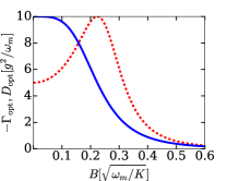
Figure 2: Optically induced damping $\Gamma_{\mathrm{opt}}$ and diffusion $D_{\mathrm{opt}}$ as a function of the amplitude $B$ for the setup with one cavity. The damping is equal to the negative diffusion, as we neglected the off-resonant terms in Eqs. (11), (16). The parameters in this plot are $\kappa/\omega_{m}=0.1$, $K/\omega_{m}\to 0$, $\Delta=\omega_{m}$ (blue solid line), $\Delta=1.1\omega_{m}$ (red dashed line).

Since we expect only small fluctuations around the mean of the amplitude distribution, we linearize the drift around $B_{0}$. Using $\Gamma_{m}+\Gamma_{\mathrm{opt}}(B_{0})=0$ we find

$$A_{B}(B)\approx A_{B}(B_{0})+\left.\frac{\mathrm{d}A_{B}}{\mathrm{d}B}\right|_{B=B_{0}}\delta B=-\Gamma_{L}\delta B\>,$$ (20)

where we defined the amplitude fluctuation $\delta B=B-B_{0}$ and the linearized damping $\Gamma_{L}=B_{0}\left.\frac{\mathrm{d}\Gamma_{\mathrm{opt}}}{\mathrm{d}B}\right|_{B=B_{0}}$. The steady-state solution Eq. (17) is then the Gaussian distribution Rodrigues and Armour (2010) $W_{B}\sim\mathrm{exp}\left(-\frac{1}{2}\frac{(\delta B)^{2}}{\sigma^{2}}\right)$ with mean $B_{0}$ and variance

$$\sigma^{2}=\frac{D(B_{0})}{2\Gamma_{L}}\>.$$ (21)

Based on this approximate solution we derive conditions under which the oscillator shows number squeezing and is therefore in a nonclassical steady state. This can be quantified by the Fano factor

$$F=\frac{\braket{n^{2}}-\braket{n}^{2}}{\braket{n}}\;,$$ (22)

the variance divided by the mean of the phonon number $n=b^{\dagger}b$. A Fano factor smaller than $1$ implies subpoissonian phonon statistics, i.e. number-state squeezing.

To derive the mechanical Fano factor, we make use of the Wigner function to calculate expectation values of symmetrically ordered products of annihilation and creation operators $b,b^{\dagger}$, e.g. $\braket{B^{2}}_{W}=\braket{n}+\frac{1}{2}$ and $\braket{B^{4}}_{W}=\braket{n^{2}}+\braket{n}+\frac{1}{2}$, where the expectation values of the operators $n$, $n^{2}$ are taken with respect to the steady-state density matrix and the expectation values of $B,B^{2}$ are with respect to the corresponding Wigner function. In the large-amplitude limit the Fano factor can then be rewritten in terms of the amplitude $B$ as $F\approx 4\sigma^{2}$.

For blue detuning we drop the non-resonant term in $D_{\mathrm{opt}}(B_{0})$ and approximate $D_{\mathrm{opt}}\approx\frac{g^{2}\kappa}{(\omega_{m}(B_{0})-\Delta)^{2}+\kappa^{2}}$. With this simplified optical diffusion we can find the steady-state variance using Eq. (21) and obtain the approximate Fano factor

$$F=\frac{(\bar{n}+1)}{2}\left(1-\frac{1}{C}+\frac{\Delta-\omega_{m}+K}{\kappa}\sqrt{\frac{1}{C}-\frac{1}{C^{2}}}\right)^{-1}\>,$$ (23)

which for large cooperativity $C\gg 1$ is limited by $F\leq\frac{(\bar{n}+1)}{2}$.

We find that squeezed number states can be achieved for bath occupation $\bar{n}<1$. Such small temperatures can be achieved with cryogenic cooling for high mechanical frequencies, but also optomechanical sideband cooling via radiation pressure. This motivates to investigate the case where the oscillator is driven by two lasers, one blue-detuned like here and one red-detuned for additional cooling, in the following Section 3.

III Two cavities

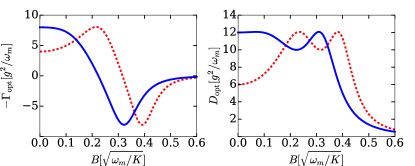
Figure 3: Optically induced damping $\Gamma_{\mathrm{opt}}$ and diffusion $D_{\mathrm{opt}}$ as a function of the amplitude $B$ for the setup with two lasers fulfilling $\Delta_{2}+\Delta_{1}=-2\kappa$. As in Fig. 2, the off-resonant terms have been neglected. The parameters in this plot are $\kappa/\omega_{m}=0.1$, $K/\omega_{m}\to 0$, $\Delta_{1}=\omega_{m}$ (blue solid line), $\Delta_{1}=1.1\omega_{m}$ (red dashed line).

We now consider the setup depicted in Fig.  1 (b), where a mechanical mode coupled to two cavity modes $a_{1},a_{2}$. For simplicity, we will here assume these modes to be in separate cavities and discuss the corrections arising for the case of a single cavity driven by two independent lasers in Section IV.2. The laser drive in the first cavity is assumed to be blue-detuned and the laser in the second cavity red-detuned, i.e. $\Delta_{1}>0>\Delta_{2}$. The second cavity will then induce (positive) optical damping and the first cavity anti-damping. The adiabatic elimination is done in analogy to the procedure above and one finds that both optically induced drift and diffusion are given by the sum of the individual contributions from Eqs. (11) and (16), i.e., $\Gamma_{\mathrm{opt}}=\Gamma_{\mathrm{opt}}(\Delta_{1},B)+\Gamma_{\mathrm{opt}}(\Delta_{2},B)$ and $D_{\mathrm{opt}}=D_{\mathrm{opt}}(\Delta_{1},B)+D_{\mathrm{opt}}(\Delta_{2},B)$. For simplicity, we assume here identical $g$ and $\kappa$ in both cavities. The resulting damping and diffusion are illustrated in Figure 3.

We are interested in the limit cycle where the average amplitude $B_{0}$ is the stable solution to $A_{B}(B_{0})=-(\Gamma_{m}+\Gamma_{\mathrm{opt}}(B_{0}))B_{0}=0$. We approximate the optically induced damping by dropping the non-resonant terms, i.e. $\Gamma_{\mathrm{opt}}(B_{0})\approx g^{2}\kappa\left(\frac{1}{(\omega_{m}(B_{0})+\Delta_{2})^{2}+\kappa^{2}}-\frac{1}{(\omega_{m}(B_{0})-\Delta_{1})^{2}+\kappa^{2}}\right)$. Assuming a large cooperativity $C\gg 1$, we can neglect the mechanical damping and obtain the average amplitude

$$B_{0}=\frac{1}{2}\sqrt{\frac{\Delta_{1}-\Delta_{2}-2\omega_{m}+2K}{K}}\>,$$ (24)

valid for $\Delta_{1}-\Delta_{2}-2\omega_{m}+2K>0$. The attractor at $B_{0}$ is only stable if $|\Delta_{1}|<|\Delta_{2}|$ and therefore only then a limit cycle will form. In the following we assume this condition to be satisfied.

In analogy to the last section, we approximate the steady-state solution of the amplitude distribution to be a Gaussian centered at $B_{0}$. Assuming a large thermal cooperativity, we neglect the mechanically induced diffusion term $\propto\Gamma_{m}(2\bar{n}+1)$. We also drop the non-resonant terms in the optically induced diffusion so that $D_{\mathrm{opt}}(B_{0})={g^{2}\kappa}\left(\frac{1}{(\omega_{m}(B_{0})-\Delta_{1})^{2}+\kappa^{2}}+\frac{1}{(\omega_{m}(B_{0})+\Delta_{2})^{2}+\kappa^{2}}\right)$. In coordinates $\Delta_{+}=\Delta_{1}+\Delta_{2}$ and $\Delta_{-}=\Delta_{1}-\Delta_{2}-2\omega_{m}+2K$, the Fano factor is then given by

$$\begin{split}F=\frac{D_{\mathrm{opt}}(B_{0})}{B_{0}\left.\frac{d\Gamma_{\mathrm{opt}}}{dB}\right|_{B=B_{0}}}=-\frac{1}{4}\frac{\Delta_{+}^{2}+4\kappa^{2}}{\Delta_{+}\Delta_{-}}\>.\end{split}$$ (25)

We optimize the detunings to achieve a minimal Fano factor: With respect to $\Delta_{+}$ it is minimal at $\frac{\mathrm{d}\sigma^{2}}{\mathrm{d}\Delta_{+}}=0$, resulting in $\Delta_{1}+\Delta_{2}=\pm 2\kappa$. Note that $\Delta_{-}$ is always positive since this is the condition to find the attractor $B_{0}$. Thus, $\Delta_{+}$ must be negative, otherwise we would get a negative variance. We therefore choose the solution with the negative sign, i.e., $\Delta_{1}+\Delta_{2}=-2\kappa.$ We find the minimal Fano Factor with respect to $\Delta_{+}$ as

$$F=\frac{\kappa}{2(\Delta_{1}-\omega_{m}+\kappa+K)}\>.$$ (26)

Subpoissonian states ($F<1$) are achieved for a wide set of parameters. In particular for $\Delta_{1}\geq\omega_{m}$ we find non-classical states for any value of $\kappa$, as long as the sidebands are resolved. In case of small nonlinearities $K\ll\kappa$ the Fano factor is independent of $K$ in both (23) and (26).

For the system with one laser in Eq. (23) we found $F=\frac{1}{2}$ for zero temperature and large cooperativity. In the system with two lasers we can achieve even smaller Fano factors by increasing the detuning, but note that the self-oscillation will not start for too large $\Delta_{1}$. In both systems the steady state amplitude scales as $B_{0}^{2}\propto 1/K$.

IV Discussion

IV.1 Comparison to Numerical Results

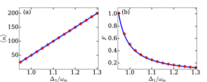
Figure 4: Comparison of analytical approximation from Eqs.  (24) and (26) to numerical results of (a) mean $\langle n\rangle=\langle b^{\dagger}b\rangle$ and (b) Fano factor $F=\Delta^{2}n/\langle n\rangle$ of the mechanical oscillator in steady state for the setup with two lasers. Here the second laser is tuned to the optimal value $\Delta_{2}=-\Delta_{1}-2\kappa$ to achieve a small Fano factor. The other parameters in this plot are $n_{\mathrm{th}}=0$ and $(K,g,\kappa,\Gamma_{m})/\omega_{m}=(0.001,0.001,0.1,0)$.

In Fig. 4 we compare our analytical findings of the mean squared amplitude and variance with an exact numerical solution of the quantum master equation for the setup with two cavities. We used three states for each cavity and 60 states for the mechanical oscillator in the steady-state solver of QuTiP Johansson et al. (2011, 2013). The results are plotted as a function of the cavity decay rate ${\kappa}/{\omega_{m}}$ and detuning of the first laser ${\Delta_{1}}/{\omega_{m}}$. The detuning of the second laser is chosen at the optimal value $\Delta_{2}=-\Delta_{1}-2\kappa$. We assumed a high-$Q$ oscillator, so that the intrinsic damping is weak compared to the optically induced damping. The effective optomechanical coupling was chosen as ${g}/{\omega_{m}}=0.001$ so that the condition for adiabatic elimination is approximately fulfilled. While we are interested here in the limit of small Kerr nonlinearities, we choose ${K}/{\omega_{m}}=0.001$ not too small to keep the Hilbert space small, cf. Eq. (24). Our analytical expression leads to values for the Fano factor that are in excellent agreement with the numerical results.

IV.2 Possible Implementations

In this article we described an ideal system, which yields the simplest analytical description. Depending on the concrete experimental implementation, one has to take into account further corrections, which we discuss in this section.

Intrinsic Nonlinearity.- We assumed a nonlinearity of Kerr type yielding a term $K(b^{\dagger}b)^{2}$ in the Hamiltonian. For mechanical oscillators, including also trapped-ion potentials, this stems from a Duffing potential $D(b+b^{\dagger})^{4}$ after a rotating-wave approximation. The rotating-wave approximation is valid for $K\ll\omega_{m}$ and $2K\braket{b^{\dagger}b}\ll\omega_{m}$, where $K=6D$. For the system in Section II, i.e. a mechanical oscillator coupled to a driven cavity, we find the condition in the steady state $2K\braket{b^{\dagger}b}\approx\Delta-\omega_{m}+K+\kappa\sqrt{C-1}\ll\omega_{m}.$ For the two-laser system with optimal detuning relation $\Delta_{1}+\Delta_{2}=-2\kappa$ we analogously derive the condition $\Delta_{1}-\omega_{m}+K+\kappa\ll\omega_{m}$. Note that we found in Eqs. (23) and (26) the smallest Fano factor for large detuning $\Delta$ or $\Delta_{1}$, but the rotating-wave approximation is only valid for detuning not much larger than $\omega_{m}$. Outside the regime of validity for the rotating wave approximation the Fano factor will significantly larger for a Duffing oscillator than expected from the Kerr-approximation.

Single Cavity.- Instead of driving two separate cavities as proposed in Section 3, it may be experimentally simpler to drive a single cavity with two laser tones. The beat between these two frequencies results in additional drift and diffusion terms, which interestingly are phase-dependent. The new terms are of the same magnitude as the terms stemming from the individual lasers, but they rotate at a frequency $\delta=\Delta_{1}-\Delta_{2}-2\omega_{m}(B)$. Therefore we may neglect these terms in a rotating-wave approximation if $\delta$ is much larger than the optically induced damping and diffusion, corresponding to $\delta\gg g^{2}/\kappa$. On the other hand, tuning $\delta=0$ can lead to rich dynamics in the limit cycle such as a phase-dependent diffusion and damping and therefore phase-dependent squeezing.

Excitation via Two-Level-Systems.- Self-oscillators can also be driven by a two-level system instead of a bosonic mode. In the Hamiltonian this corresponds to a replacement of the annihilation operator $a$ by the Pauli lowering operator $\sigma_{-}$. For example, mechanical oscillations of ions can be excited via a cycling transition Vahala et al. (2009). The results presented above can be transferred to this situation: As we used in the adiabatic elimination only the lowest-order terms in perturbation theory $\propto g^{2}$, this model is restricted to the lowest two Fock levels of the fast-decaying mode $a$. Therefore adiabatically eliminating a two-level system yields identical analytical results.

Anharmonic Mechanical Oscillators.- The most important property of our proposal is the intrinsic mechanical Duffing nonlinearity. Such nonlinearities can be engineered for example in oscillators made from graphene and carbon nanotubes Eichler et al. (2011); Singh et al. (2014). Coupling the oscillator to an auxiliary highly nonlinear system, there have been several proposals to achieve extremely large mechanical nonlinearities Jacobs and Landahl (2009); Rips et al. (2014); Lü et al. (2015), even on the order of $K/\omega_{m}\approx 0.01-0.1$. On this frontier a Duffing nonlinearity tunable by a SQUID was demonstrated in a recent experiment Ella et al. (2015). For the motion of trapped ions such high anharmonicities of the trapping potential can already be achieved with current systems Home et al. (2011).

IV.3 Conclusion and Outlook

We derived a semiclassical analytical model to characterize self-oscillations for the standard linear optomechanical system with an additional anharmonicity of the mechanical potential. We find excellent agreement with numerical simulations of the system. The main result is the prediction of a Fano factor $F=\tfrac{1}{2}{\kappa}/{(\Delta_{1}-\omega_{m}+\kappa+K)}$ for a setup using two laser tones at detunings $\Delta_{1}\approx\omega_{m}$ and $\Delta_{2}=-\Delta_{1}-2\kappa$ in the vicinity of the sidebands. For such parameters the Fano factor is nonclassical.

The model derived here can be generalized to other self-oscillators with Duffing nonlinearity such as trapped-ion systems or superconducting circuits. While we have focused on the amplitude and in particular its steady-state distribution, it will be interesting to describe the phase dynamics in future studies to examine synchronization in the quantum regime.

V Acknowledgments

We would like to acknowledge helpful discussions with E. Amitai, G. Hegi, A. Mokhberi, A. Nunnenkamp, S. Willitsch, and H. Zoubi. This work was financially supported by the Swiss SNF and the NCCR Quantum Science and Technology.

References

- Joos et al. (2003) E. Joos, H. D. Zeh, C. Kiefer, D. J. W. Giulini, J. Kupsch, and I.-O. Stamatescu, Decoherence and the Appearance of a Classical World in Quantum Theory (Springer, 2003).
- Zurek (2003) W. H. Zurek, Reviews of Modern Physics 75, 715 (2003).
- Poyatos et al. (1996) J. Poyatos, J. Cirac, and P. Zoller, Physical Review Letters 77, 4728 (1996).
- Nielsen and Chuang (2010) M. A. Nielsen and I. L. Chuang, Quantum Computation and Quantum Information (Cambridge University Press, 2010).
- Mari and Eisert (2012) A. Mari and J. Eisert, Physical review letters 109, 230503 (2012).
- Bassi et al. (2013) A. Bassi, K. Lochan, S. Satin, T. P. Singh, and H. Ulbricht, Reviews of Modern Physics 85, 471 (2013).
- Krauter et al. (2011) H. Krauter, C. A. Muschik, K. Jensen, W. Wasilewski, J. M. Petersen, J. I. Cirac, and E. S. Polzik, Physical review letters 107, 080503 (2011).
- Murch et al. (2012) K. W. Murch, U. Vool, D. Zhou, S. J. Weber, S. M. Girvin, and I. Siddiqi, Physical Review Letters 109, 183602 (2012).
- Shankar et al. (2013) S. Shankar, M. Hatridge, Z. Leghtas, K. M. Sliwa, A. Narla, U. Vool, S. M. Girvin, L. Frunzio, M. Mirrahimi, and M. H. Devoret, Nature 504, 419 (2013).
- Kienzler et al. (2015) D. Kienzler, H.-Y. Lo, B. Keitch, L. de Clercq, F. Leupold, F. Lindenfelser, M. Marinelli, V. Negnevitsky, and J. P. Home, Science (New York, N.Y.) 347, 53 (2015).
- Kronwald et al. (2013) A. Kronwald, F. Marquardt, and A. A. Clerk, Physical Review A 88, 063833 (2013).
- Wollman et al. (2015) E. E. Wollman, C. U. Lei, A. J. Weinstein, J. Suh, A. Kronwald, F. Marquardt, A. A. Clerk, and K. C. Schwab, Science 349, 952 (2015).
- Pirkkalainen et al. (2015) J.-M. Pirkkalainen, E. Damskägg, M. Brandt, F. Massel, and M. A. Sillanpää, Physical Review Letters 115, 243601 (2015).
- Lecocq et al. (2015) F. Lecocq, J. Clark, R. Simmonds, J. Aumentado, and J. Teufel, Physical Review X 5, 041037 (2015).
- Rips et al. (2012) S. Rips, M. Kiffner, I. Wilson-Rae, and M. J. Hartmann, New Journal of Physics 14, 023042 (2012).
- Golubev and Sokolov (1984) Y. M. Golubev and I. V. Sokolov, Journal of Experimental and Theoretical Physics 60, 234 (1984).
- McKeever et al. (2003) J. McKeever, A. Boca, A. D. Boozer, J. R. Buck, and H. J. Kimble, Nature 425, 268 (2003).
- Marquardt et al. (2006) F. Marquardt, J. Harris, and S. Girvin, Physical Review Letters 96, 103901 (2006).
- Rodrigues and Armour (2010) D. A. Rodrigues and A. D. Armour, Phys. Rev. Lett. 104, 053601 (2010).
- Qian et al. (2012) J. Qian, A. A. Clerk, K. Hammerer, and F. Marquardt, Physical Review Letters 109, 253601 (2012).
- Armour and Rodrigues (2012) A. D. Armour and D. A. Rodrigues, Comptes Rendus Physique 13, 440 (2012).
- Nation (2013) P. D. Nation, Physical Review A 88 (2013).
- Lörch et al. (2014) N. Lörch, J. Qian, A. Clerk, F. Marquardt, and K. Hammerer, Physical Review X 4, 011015 (2014).
- Lörch and Hammerer (2015) N. Lörch and K. Hammerer, Physical Review A 91, 061803 (2015).
- Vahala et al. (2009) K. Vahala, M. Herrmann, S. Knünz, V. Batteiger, G. Saathoff, T. W. Hänsch, and T. Udem, Nature Physics 5, 682 (2009).
- Knünz et al. (2010) S. Knünz, M. Herrmann, V. Batteiger, G. Saathoff, T. W. Hänsch, K. Vahala, and T. Udem, Physical review letters 105, 013004 (2010).
- Aspelmeyer et al. (2014) M. Aspelmeyer, T. J. Kippenberg, and F. Marquardt, Reviews of Modern Physics 86, 1391 (2014).
- Gardiner and Zoller (2004) C. Gardiner and P. Zoller, Quantum Noise (Springer, 2004).
- Carmichael (1999) H. J. Carmichael, Statistical Methods in Quantum Optics 1 (Springer, 1999).
- Walls and Milburn (2008) D. F. Walls and G. J. Milburn, Quantum Optics (Springer, 2008).
- Balanov et al. (2008) A. Balanov, N. Janson, D. Postnov, and O. Sosnovtseva, Synchronization: From Simple to Complex (Springer, 2008) p. 426.
- Johansson et al. (2011) J. R. Johansson, P. D. Nation, and F. Nori, Computer Physics Communications 183, 16 (2011).
- Johansson et al. (2013) J. Johansson, P. Nation, and F. Nori, Computer Physics Communications 184, 1234 (2013).
- Eichler et al. (2011) A. Eichler, J. Moser, J. Chaste, M. Zdrojek, I. Wilson-Rae, and A. Bachtold, Nature nanotechnology 6, 339 (2011).
- Singh et al. (2014) V. Singh, S. J. Bosman, B. H. Schneider, Y. M. Blanter, A. Castellanos-Gomez, and G. A. Steele, Nature nanotechnology 9, 820 (2014).
- Jacobs and Landahl (2009) K. Jacobs and A. J. Landahl, Physical review letters 103, 067201 (2009).
- Rips et al. (2014) S. Rips, I. Wilson-Rae, and M. J. Hartmann, Physical Review A 89, 013854 (2014).
- Lü et al. (2015) X.-Y. Lü, J.-Q. Liao, L. Tian, and F. Nori, Physical Review A 91, 013834 (2015).
- Ella et al. (2015) L. Ella, D. Yuvaraj, O. Suchoi, O. Shtempluk, and E. Buks, Journal of Applied Physics 117, 014309 (2015).
- Home et al. (2011) J. P. Home, D. Hanneke, J. D. Jost, D. Leibfried, and D. J. Wineland, New Journal of Physics 13, 073026 (2011).