The algebraic properties of the space- and time-dependent one-factor model of commodities

Abstract

We consider the one-factor model of commodities for which the parameters of the model depend upon the stock price or on the time. For that model we study the existence of group-invariant transformations. When the parameters are constant, the one-factor model is maximally symmetric. That also holds for the time-dependent problem. However, in the case for which the parameters depend upon the stock price (space) the one-factor model looses the group invariants. For specific functional forms of the parameters the model admits other possible Lie algebras. In each case we determine the conditions which the parameters should satisfy in order for the equation to admit Lie point symmetries. Some applications are given and we show which should be the precise relation amongst the parameters of the model in order for the equation to be maximally symmetric. Finally we discuss some modifications of the initial conditions in the case of the space-dependent model. We do that by using geometric techniques.

Keywords: Lie point symmetries; one-factor model; prices of commodities
MSC 2010: 22E60; 35Q91

1 Introduction

Three models which study the stochastic behaviour of the prices of commodities that take into account several aspects of possible influences on the prices were proposed by E Schwartz [1] in the late nineties. In the simplest model (the so-called one-factor model) Schwartz assumed that the logarithm of the spot price followed a mean-reversion process of Ornstein–Uhlenbeck type.  The one-factor model is expressed by the following $(1+1)$ evolution equation

$$\frac{1}{2}\sigma^{2}S^{2}F_{,SS}+\kappa\left(\mu-\lambda-\log S\right)SF_{,S}-F_{,t}=0,$$ (1)

where $\kappa>0$ measures the degree of mean reversion to the long-run mean log price, $\lambda$ is the market price of risk, $\sigma$ is the standard deviation of the return on the stock, $S$ is the stock price, $\mu$ is the drift rate of $S$ and $t$ is the time. $F$ is the current value of the futures contract which depends upon the parameters $t,~{}S,$, i.e., $F=F\left(t,S\right)$.

Generally $\kappa$, $\lambda$, $\sigma$ and $\mu$ are assumed to be constants. In such a case the closed-form solution of equation (1) which satisfies the initial condition

$$F\left(0,S\right)=S$$ (2)

was given in [1]. It is

$$\ln F\left(t,S\right)=e^{-\kappa t}\ln S+\left(1-e^{-\kappa t}\right)a^{\ast}+\frac{\sigma^{2}}{4\kappa}\left(1-e^{-2\kappa t}\right)$$ (3)

with $a^{\ast}=\mu-\lambda-\frac{1}{2}\frac{\sigma^{2}}{\kappa}$.

It has been shown that the closed-form solution (3) follows from the application of Lie point symmetries. In particular it has been shown that equation (1) is of maximal symmetry, which means that it is invariant under the same group of invariance transformations (of dimension $5+1+\infty$) as that of the Black-Scholes and the Heat Conduction Equation [2]. The detailed analysis for the Lie symmetries of the three models, which were proposed by Schwartz, and the generalisation to the $n$-factor model can be found in [3]. Other Financial models which have been studied with the use of group invariants can be found in [4, 5, 6, 7, 8, 9, 10, 11, 12] and references therein.

Solution (3) is that which arises from the application of the invariant functions of the Lie symmetry vector

$$X_{sol}=\mbox{\rm e}^{\kappa t}S\partial_{S}+F\partial_{F}$$ (4)

and also leaves the initial condition invariant.

In a realistic World parameters are not constants, but vary in time and depend upon the stock price, that is, the parameters have time and “space” dependence [13, 14], where as space we mean the stock price parameters as an analogue to Physics. In this work we are interested in the case for which the parameters $\kappa$, $\lambda$, $\sigma$ and $\mu$ are space dependent, ie, are functions of $S$. We study the Lie point symmetries of the space-dependent equation (1). As we see in that case, when $\sigma_{,S}\neq 0$, there does not exist any Lie point symmetry which satisfies the initial condition (2). The Lie symmetry analysis of the time-dependent Black-Scholes-Merton equations was carried out recently in [15], it has been shown that the autonomous, and the nonautonomous Black-Scholes-Merton equation are invariant under the same group of invariant transformations, and they are maximal symmetric. The plan of the paper is as follows.

The Lie point symmetries of differential equations are presented in Section 2. In addition we prove a theorem which relates the Lie point symmetries of space-dependent linear evolution equations with the Homothetic Algebra of the underlying space which defines the Laplace operator. In Section 3 we use these results in order to study the existence of Lie symmetries of for the space-dependent one-factor model (1) and we show that the space-dependent problem is not necessarily maximally symmetric. The generic symmetry vector and the constraint conditions are given and we prove a corollary in with the space-dependent linear evolution equation is always maximally symmetric when we demand that there exist at least one symmetry of the form (4) which satisfies the Schwartz condition (2). Furthermore in section 4 we consider the time-dependence problem and we show that the model is always maximally symmetric. Finally in section 5 we discuss our results and we draw our conclusions. AppendixA completes our analysis.

2 Preliminaries

Below we give the basic definitions and properties of Lie point symmetries for differential equations and also two theorems for linear evolution equations.

2.1 Point symmetries of differential equations

By definition a Lie point symmetry, $X,$ of a differential equation

$$\Theta\left(x^{k},u,u_{,i},u_{,ij}\right)=0,$$

where the $x^{k}$ are the independent variables, $u=u\left(x^{k}\right)$ is the dependent variable and

$$u_{,i}=\frac{\partial u}{\partial x^{i}}$$

is the generator of a one-parameter point transformation under which the differential equation $\Theta$ is invariant.

Let $\left(x^{i},u\right)\rightarrow\left(\bar{x}^{i}\left(x^{k},u,\varepsilon\right),\bar{u}\left(x^{k},u,\varepsilon\right)\right)$ be a one-parameter point transformation of the independent and dependent variables with the generator of infinitesimal transformations being

$$X=\xi^{i}\left(x^{k},u\right)\partial_{i}+\eta\left(x^{k},u\right)\partial_{u}.$$ (5)

The differential equation $\Theta$ can be seen as a geometric object on the jet space $J=J\left(x^{k},u,u_{,i},u_{,ij}\right)$. Therefore we say that $\Theta$ is invariant under the one-parameter point transformation with generator, $X$, if [16]

$$\mathcal{L}_{X^{\left[2\right]}}\Theta=0.$$ (6)

or equivalently

$$\mathcal{L}_{X^{\left[2\right]}}\Theta=\lambda\Theta~{},~{}{mod}\Theta=0,$$ (7)

where $X^{\left[2\right]}$ is the second prolongation of $X$ in the space $J$. It is given by the formula

$$X^{\left[2\right]}=X+\eta_{i}\partial_{u_{,i}}+\eta_{ij}\partial_{u_{,ij}},$$ (8)

where $\eta_{i}=D_{i}\left(\eta\right)-\Psi_{,k}D_{i}\left(\xi^{k}\right)$, $\eta_{ij}=D_{j}\left(\eta_{i}\right)-u_{ki}D_{j}\xi^{k}$ and $D_{i}$ is the operator of total differentiation, ie, $D_{i}=\frac{\partial}{\partial x^{i}}+u_{,i}\frac{\partial}{\partial u}+u_{,ij}\frac{\partial}{\partial u_{,j}}+...~{}$[16]. Moreover, if condition (6) is satisfied (equivalently condition (7)), the vector field $X$ is called a Lie point symmetry of the differential equation $\Theta$.

2.2 Symmetries of linear evolution equations

A geometric method which relates the Lie and the Noether point symmetries of a class of second-order differential equations has been proposed in [18, 19]. Specifically, the point symmetries of second-order partial differential equations are related with the elements of the conformal algebra of the underlying space which defines the Laplace operator.

Similarly, for the Lie symmetries of the second-order partial differential equation,

$$\Delta u-C^{\alpha}u_{,\beta}-u_{,t}=0,$$ (9)

where

$$\Delta=\frac{1}{\sqrt{\left|g\right|}}\frac{\partial}{\partial x^{\alpha}}\left(\sqrt{\left|g\right|}g^{\alpha\beta}\frac{\partial}{\partial x^{\beta}}\right)$$

is the Laplace operator, $g_{\alpha\beta}=g\left(x^{\beta}\right)$ is a nondegenerate tensor (we call it a metric tensor)  and $C^{\alpha}=C^{\alpha}\left(x^{\beta}\right)$, the following theorem arises.

Theorem 1

The Lie point symmetries of (9) are generated by the Homothetic Group of the metric tensor $g_{\alpha\beta},~{}G_{H}$ which defines the Laplace operator $\Delta$. The general form of the Lie symmetry vector is

$$X_{L}=\left(c_{1}+2\psi_{I}\int T^{I}\left(t\right)dt\right)+\left(T^{I}\left(t\right)Y_{I}^{\alpha}\left(x^{\beta}\right)\right)\partial_{\alpha}+\left(a\left(x^{\beta},t\right)u+b\left(x^{\beta},t\right)+c_{2}u\right)\partial_{u},$$ (10)

where $\psi_{I}$ is the homothetic factor of $Y_{I}^{a}$, $\psi_{I}=0$ for the Killing vector (KV, $\psi_{I}=1$ for Homothetic vector (HV), $a\left(x^{\beta},t\right)$ and $b\left(x^{\beta},t\right)$ are solutions of (10), $Y_{I}^{\alpha}\left(x^{\beta}\right)$ is a KV/HV of $g_{\alpha\beta}$ and the following condition holds, namely,

$$T^{I}L_{Y_{I}}C_{\alpha}-T_{,t}^{I}Y_{I\alpha}-2a_{,\alpha}=0.$$ (11)

Note that $I=1,2,...,\dim G_{H}$.

Another important result for the $(1+1)$ linear evolution equation of the form of (9) is the following theorem which gives the dimension of the possible admitted algebra.

Theorem 2

The one-dimensional linear evolution equation can admits 0, 1, 3 and 5 Lie point symmetries plus the homogenous and the infinity symmetries [17].

However, as equation (9) is time independent, it admits always the autonomous symmetry $\partial_{t}$. In the following we apply theorems 1 and 2 in order to study the Lie symmetries of the space-dependent one-factor model.

3 Space dependence of the one-factor model

The space-dependent one-factor model of commodity pricing is defined by the equation

$$\frac{1}{2}\sigma\left(S\right)^{2}S^{2}F_{,SS}+\kappa\left(S\right)\left(\mu\left(S\right)-\lambda\left(S\right)-\log S\right)SF_{,S}-F_{,t}=0.$$ (12)

The parameters, $\sigma$, $\kappa$, $\mu$ and $\lambda$, depend upon the stock price, $S$.  In order to simplify equation (12) we perform the coordinate transformation $S=\mbox{\rm e}^{x}$, that is, equation (12) becomes

$$\frac{1}{2}\sigma^{2}\left(x\right)F_{,xx}+\left(\kappa\left(x\right)\left(\mu\left(x\right)-\lambda\left(x\right)-x\right)-\frac{1}{2}\sigma^{2}\left(x\right)\right)F_{,x}-F_{,t}=0$$ (13)

or

$$\Delta F+\left(\kappa\left(\mu-\lambda-x\right)-\frac{1}{2}\sigma^{2}-\frac{1}{2}\sigma\sigma_{,x}\right)F_{,x}-F_{,t}=0,$$ (14)

where $\Delta$ is the Laplace operator in the one-dimensional space with fundamental line element

$$dx^{2}=\frac{2}{\sigma^{2}\left(x\right)}dx^{2}$$ (15)

and admits a two-dimensional homothetic algebra. The gradient KV is $K^{1}=\sigma\left(x\right)\partial_{x}~{}$ and the gradient HV is $H^{2}=\sigma\left(x\right)\int\frac{1}{\sigma\left(x\right)}dx\$with homothetic factor$~{}\psi_{H}=1.$

Equation (14) is of the form of (9) where now

$$C^{x}\left(x\right)=-\left(\kappa\left(\mu-\lambda-x\right)-\frac{1}{2}\sigma^{2}-\frac{1}{2}\sigma\sigma_{,x}\right)$$ (16)

and

$$C_{x}\left(x\right)=-\frac{2\left(\kappa\left(\mu-\lambda-x\right)-\frac{1}{2}\sigma^{2}-\frac{1}{2}\sigma\sigma_{,x}\right)}{\sigma^{2}\left(x\right)}.$$ (17)

Without performing any symmetry analysis we observe that, when $C^{x}\left(x\right)=0$, (14) is in the form of the heat conduction equation and it is maximally symmetric, ie, it admits $5+1+\infty$ symmetries. In the case for which $\sigma_{,x}\neq 0$ from (16) we have that

$$\sigma^{2}\left(x\right)=\left(4\int e^{2x}K\left(x\right)\mbox{\rm d}x+c_{1}\right)e^{-2x},$$ (18)

where $K\left(x\right)=\kappa\left(x\right)\left(\mu\left(x\right)-\lambda\left(x\right)-x\right)$. However, this is only a particular case whereas new cases can arise from the symmetry analysis.

3.1 Symmetry analysis

Let $Y_{I}\left(x\right),~{}I=1,2$ be the two HVs of the space (15) with homothetic factors $\psi_{I}$. As (14) is autonomous and linear, it admits the Lie symmetries $\partial_{t},~{}F\partial_{F},~{}b\left(t,x\right)\partial_{F}$, where $b\left(t,x\right)$ is a solution of (14), Therefore from theorem 1 we have that the possible additional Lie symmetry vector is

$$X=\left(2\psi_{I}\int T^{I}\left(t\right)dt\right)+T^{I}\left(t\right)Y_{I}\partial_{x}+\left(a\left(x,t\right)F\right)\partial_{F}$$ (19)

for which the following conditions hold

$$T_{1}L_{Y_{1}}C_{x}+T_{2}L_{Y_{2}}C_{x}-T_{1,t}Y_{1}-T_{2,t}Y_{2}-2a_{,x}=0\quad\mbox{\rm and}$$ (20)

$$\Delta a-C^{x}a_{,x}-a_{,t}=0.$$ (21)

We study two cases: A) $a\left(t,x\right)=0$ and B) $a\left(t,x\right)\neq 0.$

3.1.1 Case A

Let $a\left(t,x\right)=0$. Then (21) is satisfied. Hence from (20) we have the system

$$L_{Y_{I}}C_{x}-mY_{I}=0,$$ (22)

where $T_{I,t}=mT$, ie, $T_{I}\left(t\right)=T_{01}e^{mt}$. This means that from any vector field $Y_{I}$ we have only one symmetry. Hence from Theorem 2 condition (22) should hold for $I=1$ and $I=2.$ In this case the space-dependent one-factor model admits $3+1+\infty$ Lie point symmetries.

3.1.2 Case B

Consider that $a\left(t,x\right)\neq 0$. From (20) we have that

$$a\left(t,x\right)=-\frac{1}{2}\int\left(T_{1}L_{Y_{1}}C_{x}+T_{2}L_{Y_{2}}C_{x}-T_{1,t}Y_{1}-T_{2,t}Y_{2}\right)dx+f\left(t\right)$$ (23)

and then (21) gives

$$0 = \frac{1}{2}\sigma^{2}\left(T_{1}L_{Y_{1}}C_{x}+T_{2}L_{Y_{2}}C_{x}-T_{1,t}Y_{1}-T_{2,t}Y_{2,x}\right)_{,x}+C^{x}\left(T_{1}L_{Y_{1}}C_{x}+T_{2}L_{Y_{2}}C_{x}-T_{1,t}Y_{1}-T_{2,t}Y_{2}\right)+$$ (24)

$$-\int\left(T_{1,t}L_{Y_{1}}C_{x}+T_{2,t}L_{Y_{2}}C_{x}-T_{1,tt}Y_{1}-T_{2,tt}Y_{2}\right)dx+2f\left(t\right).$$

Consider the case for which $T_{1}\neq T_{2}$. Recall that for the space (15), $Y_{I,x}=2\psi_{I},$ that is, from (24) we have the conditions

$$0 = \frac{1}{2}\sigma^{2}\left(L_{Y_{1}}C_{x}\right)_{,x}+C^{x}L_{Y_{1}}C_{x}-\frac{T_{1,t}}{T_{1}}\left(\frac{1}{2}\int L_{Y_{1}}C_{x}dx+C^{x}Y_{1}+2\psi_{1}\right)+$$ (25)

$$+\frac{1}{2}\frac{T_{1,tt}}{T_{1}}\int Y_{1}dx+2f_{1,t}\quad\mbox{\rm and}$$

$$0 = \frac{1}{2}\sigma^{2}\left(L_{Y_{2}}C_{x}\right)_{,x}+C^{x}L_{Y_{2}}C_{x}-\frac{T_{2,t}}{T_{2}}\left(\frac{1}{2}\int L_{Y_{2}}C_{x}dx+C^{x}Y_{2}+2\psi_{2}\right)+$$ (26)

$$+\frac{1}{2}\frac{T_{2,tt}}{T_{2}}\int Y_{2}dx+2f_{2,t},$$

where $f\left(t\right)=f_{1}\left(t\right)+f_{2}\left(t\right)$. We continue with the subcases:

Subcase B1

Let $T_{I,tt}=T_{I}^{0}T_{I,t}~{},~{}T_{I,t}\neq 0,$ that is, $T_{I}\left(t\right)=T_{I}^{1}+T_{I}^{2}e^{T_{I}^{0}t}$. In this case the symmetry conditions are:

$$0=\left(\frac{1}{2}\sigma^{2}\left(L_{Y_{I}}C_{x}\right)_{,x}+C^{x}L_{Y_{I}}C_{x}\right)-\frac{T_{I,t}}{T_{I}}\left(\frac{1}{2}\int L_{Y_{I}}C_{x}+C^{x}Y_{I}+2\psi_{I}+\frac{1}{2}\int Y_{I}\mbox{\rm d}x\right)+2f_{I,t}.$$ (27)

Hence we have the following system

$$\frac{1}{2}\sigma^{2}\left(L_{Y_{I}}C_{x}\right)_{,x}+C^{x}L_{Y_{I}}C_{x} = c$$ (28)

$$\frac{1}{2}\int L_{Y_{I}}C_{x}+C^{x}Y_{I}+2\psi_{I}+\frac{1}{2}\int Y_{I}\mbox{\rm d}x = m$$ (29)

$$2f_{I,t}-m\frac{T_{I,t}}{T_{I}}+c = 0.$$ (30)

If system (28)-(30) holds for $I=1$ or $I=2$, then equation (14) admits $3+1+\infty$    Lie symmetries and in the case for which conditions (28)-(30) hold, ie, admits $5+1+\infty$ Lie symmetries which is the maximum for a $(1+1)$ evolution equation.

Subcase B2

In the second subcase we consider that $T_{I,tt}\neq T_{I,t}$.

Hence, if B2.a) $T_{I,tt}=0$, then from (25) and (26) it follows that

$$\frac{1}{2}\int L_{Y_{I}}C_{x}dx+C^{x}Y_{I}+2\psi_{I}=0$$ (31)

$$\frac{1}{2}\sigma^{2}\left(L_{Y_{I}}C_{x}\right)_{,x}+C^{x}L_{Y_{I}}C_{x}=c\quad\mbox{\rm and}$$ (32)

$$2f_{I,t}+c=0,$$ (33)

where from Theorem 2 these conditions must hold for $I=1$ and $I=2$ and equation (14) is maximally symmetric.

B2.b) Let $T_{,tt}\neq 0$. Then it follows that

$$\frac{1}{2}\int L_{Y_{I}}C_{x}dx+C^{x}Y_{I}+2\psi_{I}=0,$$ (34)

$$\frac{1}{2}\sigma^{2}\left(L_{Y_{I}}C_{x}\right)_{,x}+C^{x}L_{Y_{I}}C_{x}+\frac{1}{2}m\int Y_{I}dx=c\quad\mbox{\rm and}$$ (35)

$$\frac{T_{I,tt}}{T_{I}}=m_{I}~{},~{}2f_{I,c}+c-m_{I}=0.$$ (36)

These conditions hold for $I=1$ or $I=2$. If these conditions hold for both $I=1$ and $2$, then equation (14) is maximally symmetric.

We collect the results in the following theorem.

Theorem 3

The autonomous $(1+1)$ linear equation (14), apart from the symmetry of autonomy, the linear symmetry and the infinity symmetry, can admit:

A) The two Lie symmetries $X_{I}=2\frac{\psi_{I}}{m}e^{mt}\partial_{t}+e^{mt}Y_{I}\partial_{I}$, where $Y_{I}$ is a HV of the one-dimensional flat space with $I=`1,2$ if and only if condition (22) holds for $I=1$ and $I=2$.

B1) The two or four Lie symmetries

$$X_{I}=2\psi_{I}\int T_{I}\left(t\right)dt~{}\partial_{t}+T_{I}\left(t\right)Y_{I}+\alpha\left(t,x\right)F\partial_{F}$$ (37)

if conditions (28)-(30) hold for $I=1$ or $2,$ and $I=1$ and $2$, respectively, where $T_{I}\left(t\right)=T_{I}^{1}+T_{I}^{2}e^{T_{I}^{0}t}$ and

$$a\left(t,x\right)=-\frac{1}{2}\int\left(T_{I}L_{Y_{I}}C_{x}-T_{I,t}Y_{1}\right)dx+f_{I}\left(t\right).$$ (38)

B2.a) The four Lie symmetries (37) if conditions (31)–(33) hold for $I=1$ and $2$, where $T_{I}=T_{I0}+T_{I1}t$ and $a\left(t,x\right)$ is given by (38).

B2.b) The two or four Lie symmetries (37) if and only if conditions (34)–(36) hold for $I=1$ or $2,$ and $I=1$ and $2$, respectively, where $T_{I,tt}=m_{I}T.$

Furthermore, we comment that theorem (3) holds for all linear autonomous equations of the form of (9).

Here we discuss the relation among the Lie symmetries and the initial condition (2). In the case of constant parameters, ie, in equation (1) the Lie symmetry vector (4) is the linear combination among the linear symmetry $F\partial_{F}$ and the symmetry which is generated by the KV of the underlying space, which is $K^{1}=\sigma_{0}\partial_{x},~{}$for $\sigma\left(x\right)=\sigma_{0}$. However, for a general function, $\sigma\left(S\right)$, in order for the symmetry which is generated by the KV $K^{1}$ to satisfy the initial condition $\sigma\left(S\right)=\sigma_{0}$ or the initial condition has to change.

Consider now that $Y^{1}=K^{1}$ and satisfies the conditions

$$L_{K_{1}}C_{x}=0~{},~{}C^{x}Y_{1}=0.$$ (39)

Then from theorem 3, B2.a, we have that $\sigma\left(x\right)$ is given by (18) and at the same time $Y^{2}=H$ generates two Lie point symmetries for equation (14). The Lie point symmetries are

$$X_{t}=\partial_{t},~{}X_{F}=F\partial_{F},~{}X_{1}=\sigma\left(x\right)\partial_{x},~{}X_{2}=t\sigma\left(x\right)\partial_{x}-\sigma\left(x\right)F\partial_{F},~{}$$

$$X_{3}=2t\partial_{t}+\sigma\left(x\right)\int\frac{1}{\sigma\left(x\right)}dx~{}\partial_{x}\mbox{\rm and}$$

$$X_{4}=t^{2}\partial_{t}+t\sigma\left(x\right)\int\frac{1}{\sigma\left(x\right)}dx~{}\partial_{x}-\left(\frac{1}{2}t+\left(\int\frac{1}{\sigma\left(x\right)}dx\right)^{2}\right)F\partial_{F}$$

plus the autonomous and trivial symmetries. The symmetry vector field $X_{1}$ is the KV of the one-dimensional space. Therefore, if we wish the field $\bar{X}=X_{1}+\mu X_{F}$ to satisfy an initial condition such as $F\left(0,x\right)=g\left(x\right)$, then it should be $X_{1}\left(g\left(x\right)\right)=g\left(x\right)$ which gives $g\left(x\right)=e^{\int\sigma\left(x\right)dx}$.  From this we can see that, when $\sigma\left(x\right)=\sigma_{0}$, we have the initial condition (2).

Let $\kappa$, $\lambda$ and $\mu$ be constants. Hence from (18) we have that

$$\sigma^{2}\left(x\right)=2\kappa\left(\left(\mu-\lambda\right)-x\right)+\kappa+c_{1}e^{-2x},$$ (40)

where for $c_{1}=0$ we have

$$\ln g\left(x\right)=\mp\kappa\frac{\left(2\left(\mu-\lambda-x\right)+1\right)}{3}\sigma$$ (41)

and the solution for position $\sigma\left(x\right)>0$

$$\ln F\left(t,x\right)=\frac{\mu}{2}\left(\mu\kappa t-2\sqrt{2\left(\mu-\lambda-x\right)+1}\right).$$ (42)

Let now $\sigma\left(x\right)=x$ and consider that the KV $K^{1}=x\partial_{x}$ generates a Lie point symmetry of equation (14) from Case A of theorem 3. Then from condition (22) we have that

$$xC_{,x}^{x}-C^{x}+mx=0,$$ (43)

that is,

$$C^{x}=-m\ln x+c_{1}x.$$ (44)

However, in that case, equation (14) is maximally symmetric and admits $5+1+\infty~{}$Lie point symmetries. Consider reduction with the Lie symmetry $\bar{X}=e^{mt}x\partial_{x}+F\partial_{F}$ which keeps invariant the initial condition

$$F\left(0,x\right)=\frac{1}{x}.$$ (45)

The application of $\bar{X}$ in (14) gives

$$F\left(t,x\right)=x^{\exp\left(-mt\right)}\exp\left(-\frac{1}{4m}e^{-2mt}-\frac{c_{1}}{m}e^{-mt}\right)~{},~{}m\neq 0$$ (46)

$$F\left(t,x\right)=x\exp\left(\left(c_{1}+\frac{1}{2}\right)t\right)~{},~{}m=0.$$ (47)

As another application of theorem 3 we select $\sigma\left(x\right)=e^{x}$. Then the KV $K^{1}$ is $K^{1}=e^{x}\partial_{x}$. Let this generate a Lie point symmetry for equation (14) from the case A of theorem 3, that is, conditions (22) give

$$C^{x}=-m+c_{1}e^{-x},$$ (48)

where now we can see that equation (14) is maximally symmetric and admits $5+1+\infty$ point symmetries. Consider the Lie symmetry $\bar{X}=e^{mt+x}\partial_{x}+F\partial_{F}$, which leaves invariant the modified initial condition $F\left(0,x\right)=x$. The invariant solution which follows is

$$\ln\left(F,x\right)=-\frac{e^{-mt}}{4m}\left(4me^{-x}-4c+e^{-mt}\right).$$

We observe that, when $K^{1}$ generates a Lie point symmetry for equation (14), the functional form of $C^{x}$, which includes $\kappa\left(x\right),\lambda\left(x\right)$ and $\mu\left(x\right)$ has a specific form, such that equation (14) is maximally symmetric and equivalent with the Black-Scholes and the Heat equations. In general, for unknown function $\sigma\left(x\right)$, from theorem 1 we have the following corollary.

Corollary 4

When the KV of the underlying space which defines the Laplace operator in equation (14) generates a Lie point symmetry, the functional form of $C^{x}$ is

$$C^{x}\left(x\right)=\sigma\left(x\right)\int\frac{m}{\sigma\left(x\right)}dx+c\sigma\left(x\right)$$ (49)

and equation (14) is maximally symmetric. The symmetry vectors, among the autonomous, the homogeneous and the infinity symmetries, are:

$$Z^{1}=e^{mt}K^{1}~{},~{}Z^{2}=e^{-mt}\left(K^{1}+m\int\frac{dx}{\sigma\left(x\right)}F\partial_{F}\right)$$ (50)

$$Z^{3}=e^{2mt}\left(\partial_{t}+H\right)$$ (51)

$$Z^{4}=e^{-2mt}\left(\partial_{t}-H-m\left(2m\left(\int\frac{dx}{\sigma\left(x\right)}\right)^{2}-1\right)F\partial_{F}\right)$$ (52)

for $m\neq 0$, $c=0$,

$$Z^{1}=e^{mt}K_{1}~{},~{}Z^{2}=e^{-mt}\left(K^{1}+\left(m\int\frac{dx}{\sigma\left(x\right)}+c\right)F\partial_{F}\right)$$ (53)

$$Z^{3}=e^{2mt}\left(\partial_{t}+H+cK^{1}\right)$$ (54)

$$Z^{4}=e^{-2mt}\left(\partial_{t}-H-cK^{1}+\left(2m^{2}\left(\int\frac{dx}{\sigma\left(x\right)}\right)^{2}+4mc\left(\int\frac{dx}{\sigma\left(x\right)}\right)+2c^{2}-m\right)F\partial_{F}\right)$$ (55)

for $m\neq 0$, $c\neq 0,$ and

$$Z^{1}=K^{1}~{},~{}Z^{2}=tK^{1}-\left(\int\frac{dx}{\sigma\left(x\right)}F-t\right)F\partial_{F}$$ (56)

$$Z^{3}=2t\partial_{t}+H+ctK^{1}$$ (57)

$$Z^{4}=t^{2}\partial_{t}+H+\frac{t}{2c}K^{1}-\left(\frac{1}{2}\int\frac{dx}{\sigma\left(x\right)}^{2}+\frac{1}{2c}\int\frac{dx}{\sigma\left(x\right)}-ct\int\frac{dx}{\sigma\left(x\right)}+\frac{c^{2}}{2}t^{2}\right)F\partial_{F}$$ (58)

for $m=0$, $c\neq 0$, where $K_{1}=\sigma\left(x\right)\partial_{x}$ and $H=\sigma\left(x\right)\int\frac{dx}{\sigma\left(x\right)}\partial_{x}$ are the elements of the Homothetic algebra of the underlying space.

We note that corollary 4 holds for all autonomous linear 1+1 evolution equations. In the following section we discuss the group invariants of the time-dependent problem.

4 Time-dependent one-factor model

When the parameters $\sigma,~{}\kappa,\lambda$ of equation (1) depend upon time, the one-factor model can be written as

$$\frac{1}{2}\sigma^{2}(t)(F_{xx}-F_{x})+(p(t)-xq(t))F_{x}-F_{t}=0,$$ (59)

where

$$p\left(t\right)=q\left(t\right)\left(\mu\left(t\right)-\lambda\left(t\right)\right)~{},~{}q\left(t\right)=\kappa\left(t\right).$$

Without loss of generality we can select $\sigma\left(t\right)=1$.  By analysing the determining equations as provided by the Sym package [20, 21, 22] we find that the general form of the Lie symmetry vector is

$$X = a(t)\partial_{t}+\left[b(t)+\frac{a^{\prime}x}{2}\right]\partial_{x}$$ (60)

$$+\left[f(t)+\frac{1}{4}\left(4xbq+x(1-2p)a^{\prime 2}qa^{\prime}-4x(b^{\prime}+ap^{\prime})\right.\right.$$

$$\left.\left.-x^{2}(-2aq^{\prime}+a^{\prime\prime})\right)\right]F\partial_{F},$$

where functions $a\left(t\right),b\left(t\right)\,,~{}f\left(t\right)$ are given by the system of ordinary differential equations,

$$0 = -bq+2bpq-\frac{a^{\prime}}{4}+pa^{\prime 2}a^{\prime}+qa^{\prime}+$$ (61)

$$+b^{\prime}-2pb^{\prime}-2f^{\prime}+ap^{\prime}-2app^{\prime}+aq^{\prime}-\frac{a^{\prime\prime}}{2},$$

$$0 = -2bq^{2}-\frac{3}{2}qa^{\prime}+3pqa^{\prime}+2aqp^{\prime}+$$ (62)

$$+3a^{\prime}p^{\prime}-aq^{\prime}-2bq^{\prime}+2apq^{\prime}+2b^{\prime\prime}+2ap^{\prime\prime}$$

and

$$0=-2q^{2}a^{\prime}-2aqq^{\prime}-2a^{\prime}q^{\prime}-aq^{\prime\prime}+\frac{a^{\prime\prime\prime}}{2}$$

in addition to the infinite number of solution symmetries. Consequently the algebra is $\{sl(2,\Re)\oplus_{s}W_{3}\}\oplus_{s}\infty A_{1}$ so that it is related to the classical Heat Equation by means of a point transformation. In the following we discuss our results.

5 Conclusions

In the models of financial mathematics the parameters of the models are assumed to be constants. However, in real problems these parameters can depend upon the stock prices and upon time. In this work we considered the one-factor model of Schwartz and we studied the Lie symmetries in the case for which the parameters of the problem are space-dependent. In terms of Lie symmetries, the one-factor model it is maximally symmetric and it is equivalent with the Heat equation, but in the case where the parameters are space dependent, that is not necessary true, and we show that the model can admit 1, 3 or 5 Lie point symmetries (except the trivial ones). To perform this analysis we studied the Lie symmetries of the autonomous linear evolution equation and we found that there exist a unique relation among the Lie symmetries and the collineations of the underlying geometry, where as geometry we define the “space” of the second derivatives. However, for a specific relation among the parameters of the model the system is always maximally symmetric.  In particular, that holds when $\sigma\left(x\right)$ is an arbitrary function and

$$\left(\kappa\left(\mu-\lambda-x\right)-\frac{1}{2}\sigma^{2}-\frac{1}{2}\sigma\sigma_{,x}\right)=\sigma\int\frac{m}{\sigma}dx+c\sigma,$$ (63)

where $m,c$ are constants. In that case, the correspoding symmetry (4) becomes $\bar{Z}=e^{mt}\sigma\left(x\right)\partial_{x}+F\partial_{x}$.

Consider that $\sigma\left(x\right)=1+\varepsilon e^{x-x_{0}}$, and (63) holds. Then the application of the Lie symmetry $\bar{Z}$ in (14) gives the solution

$$\ln F\left(t,x\right)=-e^{-mt}\ln\left(1+\varepsilon e^{x-x_{0}}\right)+e^{-mt}\left(x-x_{0}\right)+\frac{c}{m}e^{-mt}-\frac{1}{4m}e^{-2mt},$$ (64)

where in the limit $\varepsilon\rightarrow 0$, solution (64) becomes

$$\ln F\left(t,x\right)=e^{-mt}\left(x-x_{0}\right)+\frac{c}{m}e^{-mt}-\frac{1}{4m}e^{-2mt}$$ (65)

which can compared with solution (3).

Consider now that $\sigma\left(x\right)$ is periodic around the line $\sigma_{0}=1$. Let $\sigma\left(x\right)=1+\varepsilon\sin\left(\omega x\right)$ that and (63) holds. Hence the solution of the space-dependent one-factor model (14) which follows from the Lie symmetry $\bar{Z}$ is

$$\ln F\left(t,x\right)=\frac{2e^{-mt}}{\sqrt{1+\varepsilon^{2}}}i\arctan\left(\frac{\tan\left(\frac{x}{2}\right)+\varepsilon}{\sqrt{1-\varepsilon^{2}}}\right)+\frac{c}{m}e^{-mt}-\frac{1}{4m}e^{-2mt}$$ (66)

which is a periodic function of the stock price $x$.  For $\varepsilon<<1$ the Taylor expansion of the static solution (66) around the point $\varepsilon=0$, is

$$\ln F\left(t_{0},x\right)\simeq ix+\varepsilon\cos x+O\left(\varepsilon^{2}\right).$$ (67)

In Figure 1 we give the static evolution of the solutions, (65) and (66), for various values of the constant $\varepsilon$.

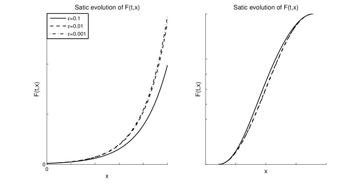
Figure 1: Evolution of the static solution (64) (left figures) and solution (66) (right. figure) for various values of the constant $\varepsilon$. Solid line is for $\varepsilon=0.1$, dash dash line is for $\varepsilon=0.1$, and the dash dot line is for $\varepsilon=0.01$.

On the other hand, in Section 4 we studied the case for which the parameters of the one-factor model are time-dependent and we showed that the model is always maximally symmetric and equivalent with the Heat Equation, that is, the time-depedence does not change the admitted group invariants of the one-factor model (1).

A more general consideration will be to extend this analysis to the two-factor and three-factor models and also to study the cases for which the parameters are dependent upon the stock price and upon the time, ie, the parameters are space and time dependent. This work is in progress.

Finally we remark how useful are the methods which are applied in Physics and especially in General Relativity for the study of space-dependent problems in financial mathematics. The reason for this is that from the second derivatives a (pseudo)Riemannian manifold can be defined. This makes the use of the methods of General Relativity and Differential Geometry essential.

Acknowledgements

The research of AP was supported by FONDECYT postdoctoral grant no. 3160121. RMM thanks the National Research Foundation of the Republic of South Africa for the granting of a postdoctoral fellowship with grant number 93183 while this work was being undertaken.

Appendix A Proof of Theorem 1

In [18] it has been shown that for a second-order PDE of the form,

$$A^{ij}\left(x^{k}\right)u_{,ij}-B^{k}(x)u_{k}=0,$$ (68)

the Lie symmetries are generated by the conformal algebra of the tensor $A^{ij}$.  Specifically the Lie symmetry conditions for equation (68) are

$$A^{ij}(a_{ij}u+b_{ij})-(a_{,i}u+b_{,i})B^{i}=0,$$ (69)

$$A^{ij}\xi_{,ij}^{k}-2A^{ik}a_{,i}+aB^{k}-\xi_{,i}^{k}B^{i}+\xi^{i}B_{,i}^{k}-\lambda B^{k}=0\quad\mbox{\rm and}$$ (70)

$$L_{\xi^{i}}A^{ij}=(\lambda-a)A^{ij},$$ (71)

where

$$\eta=a(x^{i})u+b(x^{i})~{}~{},~{}\xi^{k}=\xi^{k}(x^{i}).$$ (72)

By comparison of equations (9) and (68) we have that $x^{i}=\left(x^{\alpha},t\right),~{}A^{ij}=g^{\alpha\beta}\left(x^{\beta}\right)$, ie, $A^{tt}=A^{it}=0~{}$ and

$$B^{t}=1~{},~{}B^{\alpha}=\Gamma^{\alpha}+C^{\alpha},$$ (73)

where $\Gamma^{\alpha}=\Gamma_{\beta\gamma}^{\alpha}g^{\beta\gamma}$. Therefore the symmetry vector $X$ for equation (9) has the form

$$X=\xi^{t}\left(t\right)\partial_{t}+\xi^{\alpha}\left(t,x^{\beta}\right)\partial_{\alpha}+\left(a(x^{\alpha},t)u+b(x^{a},t)\right)\partial_{u}.$$ (74)

We continue with the solution of the symmetry conditions.

When we replace $~{}A^{ij}=g^{\alpha\beta}\left(x^{\beta}\right)$  in (71), it follows that $L_{\xi^{\alpha}}g_{\alpha\beta}=\left(\alpha-\lambda\right)g_{\alpha\beta}~{}$ which means that $\xi^{\alpha}=T^{I}\left(t\right)Y_{I}^{\alpha}\left(x^{\beta}\right)$, where $Y_{I}^{\alpha}$ is a CKV of the metric, $g_{\alpha\beta}$, with conformal factor $\psi_{I}$,  ie,$~{}\psi_{I}=\frac{1}{n}Y_{;\alpha}^{\alpha}$ and $\alpha-\lambda=2T^{I}\psi_{I}.~{}$ Furthermore, from (70) the following system follows (recall that $B_{,i}^{t}=0$ and $\xi_{,\beta}^{t}=0\,$)

$$g^{ij}\xi_{,ij}^{\alpha}-2g^{i\alpha}a_{,i}+aB^{\alpha}-\xi_{,i}^{\alpha}B^{i}+\xi^{i}B_{,i}^{\alpha}-\lambda B^{\alpha}=0\quad\mbox{\rm and}$$ (75)

$$\left(a-\lambda\right)B^{t}-\xi_{,t}^{t}B^{t}=0.$$ (76)

Moreover we observe that $\psi\left(x^{k}\right)=\psi_{I}$, where $\psi_{I}$ is a constant; that is, $Y_{I}^{\alpha}\left(x^{\beta}\right)$ is a KV/HV of $g_{\alpha\beta}$.  Finally for the function, $\xi^{t}\left(t\right),$ it holds that $\xi^{t}\left(t\right)=2\psi_{I}\int T^{I}\left(t\right)dt.~{}$

The symmetry condition (75) gives

$$g^{\beta\gamma}\xi_{,\beta\gamma}^{\alpha}-\xi_{,\gamma}^{\alpha}\Gamma^{\gamma}+\xi^{\gamma}\Gamma_{,\gamma}^{\alpha}-\xi_{,\gamma}^{\alpha}C^{\gamma}+\xi^{\gamma}C_{,\gamma}^{\alpha}-2g^{\beta\alpha}a_{,\beta}+\left(a-\lambda\right)\Gamma^{\alpha}+\left(a-\lambda\right)C^{\alpha}-\xi_{,t}^{\alpha}=0.$$ (77)

It is well known that

$$g^{\beta\gamma}\xi_{,\beta\gamma}^{\alpha}+\xi^{\gamma}\Gamma_{,\gamma}^{\alpha}-\xi_{,\gamma}^{\alpha}\Gamma^{\gamma}+\left(a-\lambda\right)\Gamma^{\alpha}=g^{\beta\gamma}\left(L_{\xi^{\alpha}}\Gamma_{\beta\gamma}^{\alpha}\right)$$ (78)

and, as $\xi^{\alpha}$ is a HV of $g_{\alpha\beta}$, $\left(L_{\xi^{\alpha}}\Gamma_{\beta\gamma}^{\alpha}\right)=0$ holds. Therefore (77) becomes

$$T^{I}\left(L_{Y_{I}^{\alpha}}C^{\alpha}+2\psi_{I}C^{\alpha}\right)-T_{,t}^{I}Y_{I}^{\alpha}-2g^{\beta\alpha}a_{,\beta}=0.$$ (79)

However, because $g_{\alpha\gamma}L_{\xi}C^{\alpha}=\delta_{\gamma}^{\beta}L_{\xi}C_{\beta}-2\psi C_{\gamma},$ condition (79) can be written as

$$T^{I}L_{Y_{I}}C_{a}-T_{,t}^{I}Y_{I\alpha}-2a_{,\beta}=0.$$ (80)

Finally from condition (69) we have the system

$$\Delta a-C^{\alpha}a_{,a}-a_{,t} = 0\quad\mbox{\rm and}$$ (81)

$$\Delta b_{\alpha\beta}-C^{\alpha}b_{,a}-b_{,t} = 0$$ (82)

which means that $a\left(x^{k},t\right)$ and $b\left(x^{k},t\right)$ are solutions of (9). We continue with the study of some special cases:

Case I: Let $T^{I}\left(t\right)=0$. Then from (11) $a_{,\beta}=0$ which means that $\alpha=a\left(t\right)$. However, from (81) we have that $\alpha\left(t\right)=a_{0}$ which gives the linear symmetry $a_{0}u\partial_{u}$. In that case from the form of $\xi^{t}$ the autonomous symmetry $\partial_{t}~{}$ arises.

Case II: For $T^{I}\left(t\right)\neq 0~{}$ the generic symmetry vector is

$$X=2\psi_{I}\int T^{I}\left(t\right)\partial_{t}+T^{I}Y_{I}^{\alpha}\partial_{\alpha}+\left(a\left(x^{\beta},t\right)\right)u\partial_{u},$$ (83)

where conditions (80) and (81) hold.

References

- [1] Schwartz ES (1997) The stochastic behaviour of commodity prices: implications for valuation and hedging The Journal of Finance 52 923-973
- [2] Gazizov RK & Ibragimov NH (1997), Lie symmetry analysis of Differential equations in Finance, Nonlinear Dynamics 17 387-407
- [3] Sophocleuous C, Leach PGL and Andriopoulos K (2008) Algebraic properties of evolution partial differential equations modelling prices of commodities Mathematical Methods in the Applied Sciences 31 679-694
- [4] Leach PGL & Andriopoulos K Newtonian economics Group Analysis of Differential Equations Ibragimov NH, Sophocleous C & Damianou PA (eds) (University of Cyprus, Nicosia, Cyprus, 2005) 134-142
- [5] Leach PGL, O’Hara JG & Sinkala W (2006) Symmetry-based solution of a model for a combination of a risky investment and a riskless investment Journal of Mathematical Analysis and Application 334 368-381
- [6] Naicker V, Andriopoulos K & Leach PGL (2005) Symmetry reductions of a Hamilton-Jacobi-Bellman Equation arising in Financial Mathematics Journal of Nonlinear Mathematical Physics 12 268-283
- [7] Sinkala W, Leach PGL & O’Hara JG (2008) Invariant properties of a general bond-pricing equation Applied Mathematics and Computation 201 95-107 (DOI: 10.1016/j.amc.207.12.008)
- [8] Sinkala W, Leach PGL & O’Hara JG (2008) Optimal system and group-invariant solutions of the Cox-Ingersoll-Ross Pricing Equation Mathematical Methods in the Applied Sciences 31 679-694 (DOI: 10.1002/maa.935)
- [9] Ibragimov NH & Soh CW (1997) Solution of the Cauchy problem for the Black-Scholes equation using its symmetries, Proceedings of the International Conference on Modern Group Analysis. MARS, Nordfjordeid, Norway.
- [10] Cimpoiasu R & Constantinescu R, (2012) New Symmetries and Particular Solutions for 2D Black-Scholes Model, Proceedings of the 7th Mathematical Physics Meeting: Summer School and Conference on Modern Mathematical Physics, Belgrade, Serbia
- [11] Lescot P (2012) Symmetries of the Black-Scholes equation, Methods Appl. Anal. 19 2 147-160
- [12] Bozhkov Y & Dimas S (2014) Group classification of a generalized Black–Scholes–Merton equation, Communications in Nonlinear Science and Numerical Simulation, 19 2200-2211
- [13] Achdou Y & Pironneau O (2005) Computational Methods for Option Pricing , Frontiers in Applied Mathematics (SIAM USA Philadelphia)
- [14] Fouque JP, Papanicolaou G & Sircar KR (2000) Derivatives in Financial Markets with Stochastic Volatility, Cambridge University Press, Cambridge
- [15] Tamizhmani KM, Krishnakumar K & Leach PGL (2014) Algebraic resolution of equations of the Black–Scholes type with arbitrary time-dependent parameters, Applied Mathematics and Computations 247 115-124
- [16] Olver PJ (1993) Applications of Lie Groups to Differential Equations, Graduate Texts in Mathematics, Volume 107, Springer-Verlag, New York
- [17] Lie S (1891) Lectures on differential equations with known infinitesimal transformations, (in German, written with the help of G Scheffers), Teubner BG, Leipzig
- [18] Paliathanasis A & Tsamparlis M (2012) Lie point symmetries of a general class of PDEs: The heat equation, Journal of Geometry and Physics 62 2443-2456
- [19] Paliathanasis A & Tsamparlis M (2014) The geometric origin of Lie point symmetries of the Schrodinger and the Klein-Gordon equations, International Journal of Geometric Methods in Modern Physics 11 1450037
- [20] Dimas S & Tsoubelis D (2005) SYM: A new symmetry-finding package for Mathematica Group Analysis of Differential Equations Ibragimov NH, Sophocleous C & Damianou PA edd (University of Cyprus, Nicosia) 64-70
- [21] Dimas S & Tsoubelis D (2006) A new Mathematica-based program for solving overdetermined systems of PDEs 8th International Mathematica Symposium (Avignon, France)
- [22] Dimas S (2008)Partial Differential Equations, Algebraic Computing and Nonlinear Systems (Thesis: University of Patras, Patras, Greece)