Whittaker-Kotel’nikov-Shannon approximation of $\varphi$-sub-Gaussian random processes
Short title: WKS approximation of $Sub_{\varphi}(\Omega)$ processes

Abstract

The article starts with generalizations of some classical results and new truncation error upper bounds in the sampling theorem for bandlimited stochastic processes. Then, it investigates $L_{p}([0,T])$ and uniform approximations of $\varphi$-sub-Gaussian random processes by finite time sampling sums. Explicit truncation error upper bounds are established. Some specifications of the general results for which the assumptions can be easily verified are given. Direct analytical methods are employed to obtain the results.

1 Introduction

Recovering a continuous function from discrete samples and assessing the information lost are the fundamental problems in sampling theory and signal processing. Whittaker-Kotel’nikov-Shannon (WKS) theorems allow the coding of a continuous band-limited signal by a sequence of its discrete samples without the loss of information. On the other hand sampling results are important not only because of signal processing applications. WKS theorems are equivalent to various fundamental results in mathematics, see, e.g., [4, 17, 35]. Therefore, they are also valuable for theoretical studies. In spite of the substantial progress in modern approximation methods (especially wavelets) WKS type expansions are still of great importance and numerous new refine results are published regularly by engineering and mathematics researchers, see, e.g., the recent volumes [18, 29, 41] in Birkhäuser’s Applied and Numerical Harmonic Analysis series.

Despite extensive investigations of sampling expansions of deterministic signals there has been remarkably little fundamental theoretical study for the case of stochastic signals. The publications [16, 32, 34], and references therein present an almost exhaustive survey of key results and approaches in stochastic sampling theory.

The development of stochastic sampling theory began with the truncation error upper bounds given by [1, 6, 33]. Using their pioneering approaches the majority of recent stochastic sampling results were obtained for harmonizable stochastic processes. Spectral representations of these stochastic processes and an inner product preserving isomorphism were used to employ deterministic sampling results and error bounds for finding mean square approximation errors for harmonizable stochastic processes, see, e.g., [1, 16, 30, 32, 33, 34] and references therein.

However, this approach is not applicable for other classes of stochastic processes or other measures of deviation. For example, for various practical applications one needs to require uniform convergence instead of the mean-square one. Also, from a practical point of view, measures of the closeness of trajectories are often more appropriate than estimates of mean-square errors in each time point. Controlling signal distortions in the mean-square sense may result in situations where relevant signal features are substantially locally distorted. Instead of small mean-square errors one may need to guarantee that the signal values have not been changed more than a certain tolerance. For example, near-lossless compression requires small user-defined tolerance levels, see [7, 15]. Also, it is often required to give an adequate description of the performance of approximations in both cases, for points where signals are relatively smooth and points where spikes occur. The uniform measure of closeness of trajectories maintains equal precision throughout the entire signal support. It indicates the necessity of elaborating special techniques. Recently a considerable attention was given to wavelet orthonormal series representations of stochastic processes. Some new results and references on convergence of wavelet expansions of random processes can be found in [22, 23]. WKS sampling is an important example of such expansions and requires specific methods and techniques.

The analysis and the approach presented in the paper contribute to these investigations in the former sampling literature. Sampling truncation errors for new classes of stochastic processes and probability metrics are given. Novel techniques to approximate sub-Gaussian random processes with given accuracy and reliability are developed. Finally, it should be mentioned that the analysis of the rate of convergence gives a constructive algorithm for determining the number of terms in the WKS expansions to ensure the uniform approximation of stochastic processes with given accuracy.

The article derives sampling results for two classes of the so-called $\varphi$-sub-Gaussian random processes. These classes play an important role in extensions of various properties of Gaussian processes to more general settings. To the best of our knowledge, the WKS expansions have never been studied for sub-Gaussian random processes and using $L_{p}([0,T])$ and uniform probability metrics. This work was intended as an attempt to obtain first results in this direction.

Note that even for the case of Gaussian processes the obtained sampling results and methodology are new. There are no known results on $L_{p}([0,T])$ and uniform sampling approximations of Gaussian processes in the literature.

The article is organized as follows. First, it generalizes some Belyaev’s results. Then, Section 3 introduces two classes of $\varphi$-sub-Gaussian random processes. Section 4 presents results on the approximation of $\varphi$-sub-Gaussian random processes in $L_{p}([0,T])$ with a given accuracy and reliability. Section 5 establishes explicit truncation error upper bounds in uniform sampling approximations of $\varphi$-sub-Gaussian random processes. Finally, short conclusions and some problems for further investigation are presented in Section 6.

We use direct analytical and probability methods to obtain all results. Some computations and plotting in Example 8 were performed by using Maple 17.0 of Waterloo Maple Inc.

In what follows $C$ denotes constants which are not important for our exposition. Moreover, the same symbol may be used for different constants appearing in the same proof.

2 Kotel’nikov-Shannon stochastic sampling

Known deterministic sampling methods often may not be appropriate to approximate stochastic processes and to estimate stochastic reconstruction errors. Since random signals play a key role in modern signal processing new refined sampling results for stochastic processes are required.

This section generalizes some results in [1] and obtains new truncation error upper bounds in the WKS sampling theorem for bandlimited stochastic processes.

Let $\mathbf{X}(t),$ $t\in\mathbf{R},$ be a stationary random process with $\mathbf{E}\mathbf{\mathbf{missing}}X(t)=0$ whose spectrum is bandlimited to $[-\Lambda,\Lambda),$ that is

$$\mathbf{B}(\tau):=\mathbf{E}\mathbf{X}(t+\tau)\mathbf{X}(t)=\int_{-\Lambda}^{\Lambda}e^{i\tau\lambda}dF(\lambda),$$

where $F(\cdot)$ is the spectral function of $\mathbf{X}(t).$ The process $\mathbf{X}(t)$ can be represented as

$$\mathbf{X}(t)=\int_{-\Lambda}^{\Lambda}e^{it\lambda}d\Phi(\lambda),$$ (1)

where $\Phi(\cdot)$ is a random measure on $\mathbb{R}$ such that $\mathbf{E}\left[\Phi(\Delta_{1})\Phi(\Delta_{2})\right]=F(\Delta_{1}\cap\Delta_{2})$ for any measurable sets $\Delta_{1},\Delta_{2}\subset\mathbb{R}.$

Then, for all $\omega>\Lambda$ there holds

$$\mathbf{X}(t)=\sum_{k=-\infty}^{\infty}\frac{\sin\left(\omega\left(t-\frac{k\pi}{\omega}\right)\right)}{\omega\left(t-\frac{k\pi}{\omega}\right)}\,\mathbf{X}\left(\frac{k\pi}{\omega}\right),$$ (2)

and the series (2) converges uniformly in mean square, see, for example, [1].

Let us consider the truncation version of (2) given by the formula

$$\mathbf{X}_{n}(t):=\sum_{k=-n}^{n}\frac{\sin\left(\omega\left(t-\frac{k\pi}{\omega}\right)\right)}{\omega\left(t-\frac{k\pi}{\omega}\right)}\,\mathbf{X}\left(\frac{k\pi}{\omega}\right).$$ (3)

In his classical paper [1] Belyaev proved a sampling theorem for random processes with bounded spectra. The key ingredient in obtaining the main result was an explicit upper bound of the reconstruction error. In the above notations, the bound can be written as

$$\mathbf{E}\left|\mathbf{X}(t)-\mathbf{X}_{n}(t)\right|^{2}\leq\frac{\mathbf{1}6\omega^{2}(2\pi+t\omega)^{2}B(0)}{\pi^{4}n^{2}\left(1-\frac{\Lambda}{\omega}\right)^{2}}.$$

Part 1 of Theorem 1 below generalizes this result, while part 2 obtains novel bounds for increments of the stochastic process $\mathbf{X}(t)-\mathbf{X}_{n}(t).$ Note that [1] has no results for increments analogous to those reported in part 2.

Theorem 1.

Let $z\in(0,1),$ $t>0,$ $s>0.$ Then

1. for $n\geq\frac{\omega t}{\pi\sqrt{z}}$ it holds that

   $$\mathbf{E}\left|\mathbf{X}(t)-\mathbf{X}_{n}(t)\right|^{2}\leq n^{-2}\,C_{n}(t),$$

   where

   $$C_{n}(t):=\mathbf{B}(0)\cdot\left(\frac{4\omega t}{\pi^{2}(1-z)}+\frac{4\left(z+1+\frac{1}{n}\right)}{\pi(1-z)^{2}\left(1-\frac{\Lambda}{\omega}\right)}\right)^{2};$$ (4)

2. for $n\geq\frac{\omega}{\pi\sqrt{z}}\max(t,s)$ it holds that

   $$\mathbf{E}\left(\mathbf{Y}_{n}(t)-\mathbf{Y}_{n}(s)\right)^{2}\leq\left(\frac{t-s}{n}\right)^{2}b_{n}(t,s),$$

   where $\mathbf{Y}_{n}(t):=\mathbf{X}(t)-\mathbf{X}_{n}(t),$

   $$b_{n}(t,s) := \mathbf{B}(0)\cdot\left(W_{n}(t,s)+\frac{Q_{n}(t,s)}{\left(1-\frac{\Lambda}{\omega}\right)}\right)^{2},$$ (5)

   $$W_{n}(t,s) := \frac{4\omega}{\pi^{2}(1-z)}\left(\omega s+1+\frac{\omega^{2}(s+t)s}{\pi^{2}n^{2}(1-z)}\right),$$

   $$Q_{n}(t,s) := \frac{2\omega}{\pi(1-z)^{2}}\left({z+1+n^{-1}}+\frac{2\omega(s+t)}{n\pi^{2}}\right).$$

Remark 1.

The parameter $z$ was introduced to provide simple expressions for the upper bounds. To guarantee a specified reconstruction accuracy the number of terms in parts 1 and 2 of Theorem 1 can be selected as $n=\lceil\frac{\omega t}{\pi\sqrt{z}}\rceil$ and $n=\lceil\frac{\omega}{\pi\sqrt{z}}\max(t,s)\rceil,$ respectively, where $\lceil x\rceil$ denotes the smallest integer not less than $x.$

To prove Theorem 1 we need two lemmata.

Lemma 1.

If $0\leq n<m$ and $\nu\in(0,1],$ then

$$\left|\sum_{k=n}^{m}\sin(k\pi\nu)\right|\leq\frac{1}{\nu}.$$

Proof.

Notice that

$$\left|\sum_{k=n}^{m}\sin(k\pi\nu)\right|=\left|\Im\left(\sum_{k=n}^{m}e^{ik\pi\nu}\right)\right|\leq\left|\sum_{k=n}^{m}e^{ik\pi\nu}\right|$$

$$=\left|\frac{e^{i(m+1)\pi\nu}-e^{in\pi\nu}}{e^{i\pi\nu}-1}\right|\leq\frac{2}{\left|e^{i\pi\nu}-1\right|}=\frac{1}{\sin\left(\frac{\pi\nu}{2}\right)}.$$

The statement of the lemma follows from the inequality $\sin(x)>\frac{2}{\pi}x,$ where $0<x<\pi/2.$ ∎

Lemma 2.

If $\{a_{k},k\in\mathbb{N}\}$ is a sequence of real numbers, $0\leq n<m,$ and $\nu\in(0,1],$ then

$$\left|\sum_{k=n}^{m}a_{k}\sin(k\pi\nu)\right|\leq\frac{1}{\nu}\left(\sum_{k=n}^{m}\left|a_{k+1}-a_{k}\right|+|a_{m+1}|\right).$$

Proof.

By the Abel transformation

$$\sum_{k=n}^{m}a_{k}\sin(k\pi\nu)=B_{m}a_{m+1}-\sum_{k=n}^{m}B_{k}\left(a_{k+1}-a_{k}\right),$$

where $B_{k}:=\sum_{l=n}^{k}\sin(l\pi\nu).$

Now, Lemma 2 follows from Lemma 1. ∎

Proof.

To prove Theorem 1 we note that it follows from the spectral representation (1) and

$$e^{it\lambda}=\sum_{k=-\infty}^{\infty}e^{ik\pi\lambda/\omega}\,\frac{\sin\left(\omega\left(t-\frac{k\pi}{\omega}\right)\right)}{\omega\left(t-\frac{k\pi}{\omega}\right)}$$

that

$$\mathbf{X}(t)-\mathbf{X}_{n}(t)=\int_{-\omega}^{\omega}\sum_{|k|>n}R_{k}(t,\lambda)d\Phi(\lambda),$$

where

$$R_{k}(t,\lambda):=e^{ik\pi\lambda/\omega}\,\frac{\sin\left(\omega\left(t-\frac{k\pi}{\omega}\right)\right)}{\omega\left(t-\frac{k\pi}{\omega}\right)}+e^{-ik\pi\lambda/\omega}\,\frac{\sin\left(\omega\left(t+\frac{k\pi}{\omega}\right)\right)}{\omega\left(t+\frac{k\pi}{\omega}\right)}$$

$$=\frac{\sin(\omega t)}{(\omega t)^{2}-(k\pi)^{2}}\left[2\omega t\cos\left(k\pi\left(1-\frac{\lambda}{\omega}\right)\right)-2ik\pi\sin\left(k\pi\left(1-\frac{\lambda}{\omega}\right)\right)\right]$$ (6)

and

$$\mathbf{E}\left|\mathbf{X}(t)-\mathbf{X}_{n}(t)\right|^{2}=\int_{-\omega}^{\omega}\left(\sum_{|k|>n}R_{k}(t,\lambda)\right)^{2}dF(\lambda).$$ (7)

Let $\lambda>0$ and $(\omega t)^{2}\leq z(n\pi)^{2},$ $z\in(0,1).$ Notice, that by (6) we obtain

$$\Im\left(\sum_{|k|>n}R_{k}(t,\lambda)\right)=-\sum_{|k|>n}\frac{2k\pi\sin(\omega t)}{(\omega t)^{2}-(k\pi)^{2}}\sin\left(k\pi\left(1-\frac{\lambda}{\omega}\right)\right).$$

Let $a_{k}:=\frac{2k\pi\sin(\omega t)}{(\omega t)^{2}-(k\pi)^{2}}.$ As $a_{k}\to 0$ when $k\to\infty,$ then it follows from Lemma 2 that

$$\left|\Im\left(\sum_{|k|>n}R_{k}(t,\lambda)\right)\right|\leq\frac{1}{1-\frac{\lambda}{\omega}}\cdot\sum_{|k|>n}|a_{k+1}-a_{k}|.$$ (8)

It follows from $(\omega t)^{2}\leq z(n\pi)^{2},$ $z\in(0,1),$ that for $k>n:$

$$|a_{k+1}-a_{k}|\leq 2\pi\left|\frac{k}{(\omega t)^{2}-(k\pi)^{2}}-\frac{k+1}{(\omega t)^{2}-((k+1)\pi)^{2}}\right|$$

$$=\frac{2\pi\left((\omega t)^{2}+k(k+1)\pi^{2}\right)}{\left((k\pi)^{2}-(\omega t)^{2}\right)\left(((k+1)\pi)^{2}-(\omega t)^{2}\right)}\leq\frac{2\pi^{3}\left(zk^{2}+k(k+1)\right)}{(k\pi)^{4}(1-z)^{2}}$$

$$\leq\frac{2\left(z+1+n^{-1}\right)}{\pi k^{2}(1-z)^{2}}.$$ (9)

Analogously one can obtain that (9) also holds for $k<-n.$

By (8) and (9) we get

$$\left|\Im\left(\sum_{|k|>n}R_{k}(t,\lambda)\right)\right|\leq\frac{1}{1-\frac{\lambda}{\omega}}\cdot\frac{4\left(z+1+n^{-1}\right)}{\pi(1-z)^{2}}\sum_{k=n+1}^{+\infty}\frac{1}{k^{2}}$$

$$\leq\frac{1}{1-\frac{\Lambda}{\omega}}\cdot\frac{4\left(z+1+n^{-1}\right)}{\pi(1-z)^{2}}\cdot\frac{1}{n}.$$ (10)

It follows from (6) that

$$\left|\Re\left(\sum_{|k|>n}R_{k}(t,\lambda)\right)\right|=\left|\sum_{|k|>n}\frac{2\omega t\sin(\omega t)}{(\omega t)^{2}-(k\pi)^{2}}\cos\left(k\pi\left(1-\frac{\lambda}{\omega}\right)\right)\right|$$

$$\leq\sum_{|k|>n}\frac{2\omega t}{(k\pi)^{2}-(\omega t)^{2}}\leq\frac{4\omega t}{\pi^{2}(1-z)}\sum_{k=n+1}^{+\infty}\frac{1}{k^{2}}\leq\frac{4\omega t}{\pi^{2}(1-z)}\cdot\frac{1}{n}.$$ (11)

Combining (10) and (11) we obtain

$$\left|\sum_{|k|>n}R_{k}(t,\lambda)\right|\leq\frac{S_{n}(t)}{n},$$

where

$$S_{n}(t):=\frac{4\omega t}{\pi^{2}(1-z)}+\frac{4\left(z+1+\frac{1}{n}\right)}{\pi(1-z)^{2}\left(1-\frac{\Lambda}{\omega}\right)}.$$

For the case $\lambda<0$ the proof is analogous.

Finally, item 1 of the theorem follows from (7) and the estimate

$$\mathbf{E}\left|\mathbf{X}(t)-\mathbf{X}_{n}(t)\right|^{2}\leq\int_{\omega}^{\omega}\frac{S_{n}^{2}(t)}{n^{2}}dF(\lambda)=\frac{S_{n}^{2}(t)}{n^{2}}\mathbf{B}(0)=\frac{C_{n}(t)}{n^{2}}.$$ (12)

Now we prove item 2 of the theorem. Similarly to (7) it holds true that

$$\mathbf{Y}_{n}(t)-\mathbf{Y}_{n}(s)=\int_{-\omega}^{\omega}\sum_{|k|>n}\left(R_{k}(t,\lambda)-R_{k}(s,\lambda)\right)d\Phi(\lambda),$$

$$\mathbf{E}\left|\mathbf{Y}_{n}(t)-\mathbf{Y}_{n}(s)\right|^{2}=\int_{-\omega}^{\omega}\left(\sum_{|k|>n}\left(R_{k}(t,\lambda)-R_{k}(s,\lambda)\right)\right)^{2}dF(\lambda).$$ (13)

Let $\lambda>0$ and $(\omega\max(t,s))^{2}\leq z(n\pi)^{2},$ $z\in(0,1).$

It follows from Lemma 2 that

$$\left|\Im\left(\sum_{|k|>n}\left(R_{k}(t,\lambda)-R_{k}(s,\lambda)\right)\right)\right|\leq\frac{1}{1-\frac{\lambda}{\omega}}\cdot\sum_{|k|>n}D_{k},$$ (14)

where

$$D_{k}:=2\pi\left|\frac{k\sin(\omega t)}{(\omega t)^{2}-(k\pi)^{2}}-\frac{k\sin(\omega s)}{(\omega s)^{2}-(k\pi)^{2}}-\frac{(k+1)\sin(\omega t)}{(\omega t)^{2}-((k+1)\pi)^{2}}+\frac{(k+1)\sin(\omega s)}{(\omega s)^{2}-((k+1)\pi)^{2}}\right|.$$

We can estimate $D_{k}$ as follows

$$D_{k}\leq 2\pi\left(\left|\sin(\omega t)-\sin(\omega s)\right|\left|\frac{k}{(\omega t)^{2}-(k\pi)^{2}}-\frac{k+1}{(\omega t)^{2}-((k+1)\pi)^{2}}\right|+|\sin(\omega s)|\right.$$

$$\left.\times\left|\frac{k}{(\omega t)^{2}-(k\pi)^{2}}-\frac{k+1}{(\omega t)^{2}-((k+1)\pi)^{2}}-\frac{k}{(\omega s)^{2}-(k\pi)^{2}}+\frac{k+1}{(\omega s)^{2}-((k+1)\pi)^{2}}\right|\right).$$

By the estimate

$$\left|\frac{(\omega s)^{2}-(\omega t)^{2}}{\left((\omega t)^{2}-(k\pi)^{2}\right)\left((\omega s)^{2}-(k\pi)^{2}\right)}\right|\leq\frac{\omega^{2}(s+t)|t-s|}{(k\pi)^{4}(1-z)^{2}}$$

we obtain

$$\left|\frac{k}{(\omega t)^{2}-(k\pi)^{2}}-\frac{k+1}{(\omega t)^{2}-((k+1)\pi)^{2}}-\frac{k}{(\omega s)^{2}-(k\pi)^{2}}+\frac{k+1}{(\omega s)^{2}-((k+1)\pi)^{2}}\right|$$

$$\leq(k+1)\left|\frac{(\omega s)^{2}-(\omega t)^{2}}{\left((\omega t)^{2}-((k+1)\pi)^{2}\right)\left((\omega s)^{2}-((k+1)\pi)^{2}\right)}\right|$$

$$+k\left|\frac{(\omega s)^{2}-(\omega t)^{2}}{\left((\omega t)^{2}-(k\pi)^{2}\right)\left((\omega s)^{2}-(k\pi)^{2}\right)}\right|\leq\frac{2\,\omega^{2}(s+t)|t-s|}{k^{3}\pi^{4}(1-z)^{2}}.$$ (15)

Therefore, by (9), (15), and the inequality

$$\left|\sin(\omega t)-\sin(\omega s)\right|\leq 2\left|\sin\left(\frac{\omega(t-s)}{2}\right)\right|\leq|t-s|\cdot\omega$$ (16)

we get

$$D_{k}\leq{}\left(\frac{2\omega|t-s|\left(z+1+n^{-1}\right)}{\pi k^{2}(1-z)^{2}}+\frac{4\omega^{2}(s+t)|t-s|}{\pi^{3}k^{3}(1-z)^{2}}\right)$$

$$=|t-s|\cdot\frac{2\omega}{\pi(1-z)^{2}}\left({z+1+n^{-1}}+\frac{2\omega(s+t)}{k\pi^{2}}\right)\cdot\frac{1}{k^{2}}.$$

Hence, it follows from (14) that

$$\left|\Im\left(\sum_{|k|>n}\left(R_{k}(t,\lambda)-R_{k}(s,\lambda)\right)\right)\right|\leq\frac{1}{1-\frac{\Lambda}{\omega}}\cdot|t-s|\cdot\frac{Q_{n}(t,s)}{n}.$$ (17)

Notice that

$$\left|\Re\left(\sum_{|k|>n}\left(R_{k}(t,\lambda)-R_{k}(s,\lambda)\right)\right)\right|=\left|\sum_{|k|>n}\left(\frac{2\omega t\sin(\omega t)}{(\omega t)^{2}-(k\pi)^{2}}-\frac{2\omega s\sin(\omega s)}{(\omega s)^{2}-(k\pi)^{2}}\right)\right.$$

$$\left.\times\cos\left(k\pi\left(1-\frac{\lambda}{\omega}\right)\right)\right|\leq 4\omega\sum_{k=n+1}^{+\infty}\Delta_{k},$$

where

$$\Delta_{k}:=\left|\frac{t\sin(\omega t)}{(\omega t)^{2}-(k\pi)^{2}}-\frac{s\sin(\omega s)}{(\omega s)^{2}-(k\pi)^{2}}\right|.$$

By (16) we estimate $\Delta_{k}$ as follows

$$\Delta_{k} \leq \left|\frac{t\sin(\omega t)-s\sin(\omega s)}{(\omega t)^{2}-(k\pi)^{2}}\right|+s\left|\frac{1}{(\omega t)^{2}-(k\pi)^{2}}-\frac{1}{(\omega s)^{2}-(k\pi)^{2}}\right|$$

$$\leq \frac{\omega^{2}s(s+t)|t-s|}{k^{4}\pi^{4}(1-z)^{2}}+\frac{|t-s|\cdot|\sin(\omega t)|+s|\sin(\omega t)-\sin(\omega s)|}{(1-z)(k\pi)^{2}}$$

$$\leq \frac{\omega^{2}s(s+t)|t-s|}{k^{4}\pi^{4}(1-z)^{2}}+|t-s|\,\frac{\omega s+1}{(1-z)(k\pi)^{2}}\leq\frac{|t-s|}{4\omega k^{2}}\,W_{n}(t,s).$$

Hence, we get

$$\left|\Re\left(\sum_{|k|>n}\left(R_{k}(t,\lambda)-R_{k}(s,\lambda)\right)\right)\right|\leq\frac{|t-s|}{n}\,W_{n}(t,s).$$ (19)

Combining (17) and (19) we obtain

$$\left|\sum_{|k|>n}\left(R_{k}(t,\lambda)-R_{k}(s,\lambda)\right)\right|\leq\frac{|t-s|}{n}\left(W_{n}(t,s)+\frac{Q_{n}(t,s)}{\left(1-\frac{\Lambda}{\omega}\right)}\right).$$

For the case $\lambda<0$ the proof is similar.

Finally, analogously to the derivations in (12), one can deduce statement 2 of the theorem from (13). ∎

3 $\varphi$-sub-Gaussian random processes

In their pioneering papers [1, 33] Belyaev and Piranashvili extended the deterministic sampling theory to classes of analytic stochastic processes. Almost all trajectories of these processes can be analytically continued. Recently, there have been considerable efforts to develop the WKS sampling theory to new classes of stochastic processes.

This section reviews the definition of $\varphi$-sub-Gaussian random processes and their relevant properties.

Tail distributions of sub-Gaussian random variables behave similarly to the Gaussian ones so that sample path properties of sub-Gaussian processes rely on their mean square regularity. One of the main classical tools to study the boundedness of sub-Gaussian processes was metric entropy integral estimates by Dudley [9]. These results were extended by Fernique [13] and Ledoux and Talagrand [28] using the generic chaining (majorizing measures) method. There is a rich and well-developed theory on bounding sub-Gaussian random variables and processes, therefore below we cite only some key publications related to our approach. Good introductions on bounding stochastic processes can be found in the classical monographs [10, 27, 28, 36, 37] and references therein. Regularity estimates under non-Gaussian assumptions were derived in [8]. A novel approach based on Malliavin derivatives was proposed in [38].

Some of these results can also be used to obtain bounds for Gaussian or sub-Gaussian random processes which are similar to the ones derived in this article. However, we employ specific results and methods for the $\varphi$-sub-Gaussian case. These methods are often simpler than the generic chaining or Malliavin-derivative-based concentration results. Moreover, they are in ready-to-use forms for the considered sampling problems.

The space of $\varphi$-sub-Gaussian random variables was introduced in the paper [24] to generalize the class of sub-Gaussian random variables defined in [19]. Various properties of the space of $\varphi$-sub-Gaussian random variables were studied in the book [5] and the article [11]. More information on sub-Gaussian and $\varphi$-sub-Gaussian random processes and their applications can be found in the publications [2, 5, 12, 14, 25, 40].

Definition 1.

[26] A continuous even convex function $\varphi(x),$ $x\in{\mathbb{R}},$ is called an Orlicz N-function, if it is monotonically increasing for $x>0$, $\varphi(0)=0,$ ${{\varphi(x)}/{x}}\to 0,$ when $x\to 0,$ and ${{\varphi(x)}/{x}}\to\infty,$ when $x\to\infty.$

Definition 2.

[26] Let $\varphi(x),x\in{\mathbb{R}},$ be an Orlicz N-function. The function $\varphi^{*}(x):=\sup_{y\in{\mathbb{R}}}(xy-\varphi(y)),$ $x\in{\mathbb{R}},$ is called the Young-Fenchel transform (also known as the Legendre transform) of $\varphi(\cdot).$

The function $\varphi^{*}(\cdot)$ is also an Orlicz N-function.

Definition 3.

[26] An Orlicz N-function $\varphi(\cdot)$ satisfies Condition Q if

$$\lim\limits_{x\rightarrow 0}{\varphi(x)}/{x^{2}}=C>0,$$

where the constant $C$ can be equal to $+\infty.$

Example 1.

The following functions are N-functions that satisfy Condition Q:

$$\varphi(x)=C{|x|^{\alpha}},\ 1<\alpha\leq 2;\quad\varphi(x)=\exp\{Cx^{2}\}-1;$$

$$\varphi(x)=\begin{cases}Cx^{2},&\mbox{if }|x|\leq 1,\\ C|x|^{\alpha},&\mbox{if }|x|>1,\end{cases}\quad\alpha>2,$$

where $C>0.$

Lemma 3.

[26] Let $\varphi(\cdot)$ be an Orlicz N-function. Then it can be represented as $\varphi(u)=\int_{0}^{|u|}f(v)\,dv,$ where $f(\cdot)$ is a monotonically non-decreasing, right-continuous function, such that $f(0)=0$ and $f(x)\to+\infty,$ when $x\to+\infty.$

Let $\{\Omega,\cal{B},\mathbf{P}\}$ be a standard probability space and $L_{p}(\Omega)$ denote a space of random variables having finite $p$-th absolute moments.

Definition 4.

[11, 24] Let $\varphi(\cdot)$ be an Orlicz N-function satisfying the Condition Q. A zero mean random variable $\xi$ belongs to the space $Sub_{\varphi}(\Omega)$ (the space of $\varphi$-sub-Gaussian random variables), if there exists a constant $a_{\xi}\geq 0$ such that the inequality $\mathbf{E}\exp\left(\lambda\xi\right)\leq\exp\left(\varphi(a_{\xi}\lambda)\right)$ holds for all $\lambda\in{\mathbb{R}}.$

The space $Sub_{\varphi}(\Omega)$ is a Banach space with respect to the norm (see [5])

$$\tau_{\varphi}\left(\xi\right):=\mathop{\sup}\limits_{\lambda\neq 0}\frac{\varphi^{\left({-1}\right)}\left({\ln\mathbf{E}\exp\left\{{\lambda\xi}\right\}}\right)}{\left|\lambda\right|},$$

where $\varphi^{\left({-1}\right)}(\cdot)$ denotes the inverse function of $\varphi(\cdot).$

If $\varphi(x)={x^{2}}/2$ then $Sub_{\varphi}(\Omega)$ is called a space of subgaussian random variables. This space was introduced in the article [19].

Definition 5.

[5] Let $\mathbf{T}$ be a parametric space. A random process $\mathbf{X}(t),$ $t\in\mathbf{T},$ belongs to the space $Sub_{\varphi}(\Omega)$ if $\mathbf{X}(t)\in Sub_{\varphi}(\Omega)$ for all $t\in\mathbf{T}.$

A Gaussian centered random process $\mathbf{X}(t),$ $t\in\mathbf{T},$ belongs to the space $Sub_{\varphi}(\Omega),$ where $\varphi(x)={x^{2}}/2$ and $\tau_{\varphi}(\mathbf{X}(t))=\left(\mathbf{E}\left|\mathbf{X}(t)\right|^{2}\right)^{1/2}.$

Definition 6.

[21] A family $\Xi$ of random variables $\xi\in Sub_{\varphi}(\Omega)$ is called strictly $Sub_{\varphi}(\Omega)$ if there exists a constant $C_{\Xi}>0$ such that for any finite set $I,$ $\xi_{i}\in\Xi,$ $i\in I,$ and for arbitrary $\lambda_{i}\in{\mathbb{R}},$ $i\in I:$

$$\tau_{\varphi}\left(\sum\limits_{i\in I}\lambda_{i}\xi_{i}\right)\leq C_{\Xi}\left(\mathbf{E}\left(\sum\limits_{i\in I}\lambda_{i}\xi_{i}\right)^{2}\right)^{1/2}.$$

$C_{\Xi}$ is called a determinative constant. The strictly $Sub_{\varphi}(\Omega)$ family will be denoted by $SSub_{\varphi}(\Omega).$

Definition 7.

[21] A $\varphi$-sub-Gaussian random process $\mathbf{X}(t),$ $t\in\mathbf{T},$ is called strictly $Sub_{\varphi}(\Omega)$ if the family of random variables $\{\mathbf{X}(t),t\in\mathbf{T}\}$ is strictly $Sub_{\varphi}(\Omega).$ The determinative constant of this family is called a determinative constant of the process and denoted by $C_{\mathbf{X}}$.

A Gaussian centered random process $\mathbf{X}(t),$ $t\in\mathbf{T},$ is a $SSub_{\varphi}(\Omega)$ process, where $\varphi(x)={x^{2}}/2$ and the determinative constant $C_{\mathbf{X}}=1.$

4 Approximation in $L_{p}([0,T])$

This section presents results on the WKS approximation of $Sub_{\varphi}(\Omega)$ and $SSub_{\varphi}(\Omega)$ random processes in $L_{p}([0,T])$ with a given accuracy and reliability. Various specifications of the general results are obtained for important scenarios. Notice, that the approximation in $L_{p}([0,T])$ investigates the closeness of trajectories of $\mathbf{X}(t)$ and $\mathbf{X}_{n}(t),$ see, e.g., [20, 22, 23]. It is different from the known $L_{p}$-norm results which give the closeness of $\mathbf{X}(t)$ and $\mathbf{X}_{n}(t)$ distributions for each $t,$ see, e.g., [16, 30, 31].

First, we state some auxiliary results that we need for Theorems 3 and 4.

Let $\{\mathbf{T},\mathfrak{S},\mu\}$ be a measurable space and $\mathbf{X}(t),$ $t\in\mathbf{T},$ be a random process from the space $Sub_{\varphi}(\Omega).$ We will use the following notation $\tau_{\varphi}(t):=\tau_{\varphi}\left(\mathbf{X}(t)\right)$ for the norm of $\mathbf{X}(t)$ in the space $Sub_{\varphi}(\Omega).$

There are some general results in the literature which can be used to obtain asymptotics of the tail of power functionals of sub-Gaussian processes, see, for example, [3]. In contrast to these asymptotic results, numerical sampling applications require non-asymptotic bounds with an explicit range over which they can be used. The following theorem provides such bounds for the case of $\varphi$-sub-Gaussian processes.

Theorem 2.

[20] Let $p\geq 1$ and

$$c:=\int_{\mathbf{T}}\left(\tau_{\varphi}(t)\right)^{p}\,d\mu(t)<\infty.$$

Then the integral $\int_{\mathbf{T}}\left|\mathbf{X}(t)\right|^{p}\,d\mu(t)$ exists with probability 1 and the following inequality holds

$$\mathbf{P}\left\{\int_{\mathbf{T}}\left|\mathbf{X}(t)\right|^{p}\,d\mu(t)>\varepsilon\right\}\leq 2\exp\left\{-\varphi^{*}\left(\left({\varepsilon}/c\right)^{1/p}\right)\right\}$$ (20)

for each non-negative

$$\varepsilon>c\cdot\left(f\left(p(c/\varepsilon)^{1/p}\right)\right)^{p},$$ (21)

where $f(\cdot)$ is a density of $\varphi(\cdot)$ defined in Lemma 3.

Example 2.

Let $\varphi(x)={|x|^{\alpha}}/\alpha,$ $1<\alpha\leq 2.$ Then $f(x)=x^{\alpha-1}$ and $\varphi^{*}(x)={|x|^{\gamma}}/\gamma,$ where $\gamma\geq 2$ and $1/{\alpha}+1/{\gamma}=1.$ Hence, inequality (21) can be rewritten as

$$\varepsilon>c\cdot\left(f\left(p(c/\varepsilon)^{1/p}\right)\right)^{p}=c^{\alpha}p^{(\alpha-1)p}\varepsilon^{1-\alpha}.$$

Therefore, it holds

$$\mathbf{P}\left\{\int_{\mathbf{T}}\left|\mathbf{X}(t)\right|^{p}\,d\mu(t)>\varepsilon\right\}\leq 2\exp\left\{-\frac{1}{\gamma}\left(\frac{\varepsilon}{c}\right)^{\gamma/p}\right\},$$ (22)

when $\varepsilon>c\cdot p^{\frac{\alpha-1}{\alpha}p}.$

Example 3.

If $\mathbf{X}(t),$ $t\in\mathbf{T},$ is a Gaussian centered random process, then the inequality

$$\mathbf{P}\left\{\int_{\mathbf{T}}\left|\mathbf{X}(t)\right|^{p}\,d\mu(t)>\varepsilon\right\}\leq 2\exp\left\{-\frac{1}{2}\left(\frac{\varepsilon}{\tilde{c}}\right)^{2/p}\right\}$$ (23)

holds true for $\varepsilon>\hat{c}\cdot p^{\frac{p}{2}},$ where $\hat{c}:=\int_{\mathbf{T}}\left(\mathbf{E}\left(\mathbf{X}(t)\right)^{2}\right)^{p/2}\,d\mu(t).$

Example 4.

Let $\mathbf{X}(t)$ be a centered bounded random variable for all $t\in\mathbf{T}.$ Then the process $\mathbf{X}(t),$ $t\in\mathbf{T},$ belongs to all spaces $Sub_{\varphi}(\Omega)$ and satisfies (20), (22), and (23).

Example 5.

Let $\alpha\geq 2$ and

$$\varphi(x)=\begin{cases}x^{2}/\alpha,&\mbox{if }|x|\leq 1,\\ |x|^{\alpha}/\alpha,&\mbox{if }|x|>1.\end{cases}$$

Then $\varphi(x)$ is an Orlicz N-function satisfying the Condition Q.

Let, for each $t\in\mathbf{T},$ $\mathbf{X}(t)$ be a two-sided Weibull random variable, i.e.

$$\mathbf{P}\left\{\mathbf{X}(t)\geq x\right\}=\mathbf{P}\left\{\mathbf{X}(t)\leq-x\right\}=\frac{1}{2}\exp\left\{-\frac{x^{\alpha}}{\alpha}\right\},\quad x>0.$$

Then $\mathbf{X}(t),$ $t\in\mathbf{T},$ is a random process from the space $Sub_{\varphi}(\Omega)$ and Theorem 2 holds true for

$$f(v)=\begin{cases}2v/\alpha,&\mbox{if }|v|<1,\\ |v|^{\alpha-1},&\mbox{if }|v|\geq 1,\end{cases}\quad\mbox{and}\quad\varphi^{*}(x)=\begin{cases}\alpha x^{2}/4,&\mbox{if }0\leq|x|\leq{2}/{\alpha},\\ |x|-{1}/{\alpha},&\mbox{if }{2}/{\alpha}<|x|\leq 1,\\ |x|^{\gamma}/\gamma,&\mbox{if }|x|>1,\end{cases}$$

where $\gamma\in(1,2]$ and $1/\alpha+1/\gamma=1.$

Theorem 3.

Let $\omega>\Lambda>0,$ $n\geq\frac{\omega t}{\pi\sqrt{z}},$ $z\in(0,1).$ Let $\mathbf{X}(t),$ $t\in\mathbf{R},$ be a stationary $SSub_{\varphi}(\Omega)$ process which spectrum is bandlimited to $[-\Lambda,\Lambda),$ $\mathbf{X}_{n}(t)$ be defined by (3), and

$$S_{n,p}:=\left(\frac{C_{\mathbf{X}}}{n}\right)^{p}\int_{0}^{T}C_{n}^{p/2}(t)\,dt,$$

where $C_{\mathbf{X}}$ is a determinative constant of the process $\mathbf{X}(t),$ $C_{n}(t)$ is given by (4).

Then, $\int_{0}^{T}\left|\mathbf{X}(t)-\mathbf{X}_{n}(t)\right|^{p}\,dt$ exists with probability 1 and the following inequality holds true for $\varepsilon>S_{n,p}\cdot\left(f\left(p\,(S_{n,p}/\varepsilon)^{1/p}\right)\right)^{p}:$

$$\mathbf{P}\left\{\int_{0}^{T}\left|\mathbf{X}(t)-\mathbf{X}_{n}(t)\right|^{p}\,dt>\varepsilon\right\}\leq 2\exp\left\{-\varphi^{*}\left(\left({\varepsilon}/S_{n,p}\right)^{1/p}\right)\right\}.$$

Proof.

It follows from (3) and Definition 6 that $\mathbf{X}(t)-\mathbf{X}_{n}(t)$ is a $SSub_{\varphi}(\Omega)$ random process with the determinative constant $C_{\mathbf{X}}.$

Applying Theorem 2 to $\mathbf{X}(t)-\mathbf{X}_{n}(t)$ for the case $\mathbf{T}=[0,T]$ and the Lebesgue measure $\mu$ on $[0,T]$ we obtain that $\int_{0}^{T}\left|\mathbf{X}(t)-\mathbf{X}_{n}(t)\right|^{p}\,dt$ exists with probability 1 and

$$\mathbf{P}\left\{\int_{0}^{T}\left|\mathbf{X}(t)-\mathbf{X}_{n}(t)\right|^{p}\,dt>\varepsilon\right\}\leq 2\exp\left\{-\varphi^{*}\left(\left({\varepsilon}/c\right)^{1/p}\right)\right\},$$

where $c:=\int_{0}^{T}\left(\tau_{\varphi}(\mathbf{X}(t)-\mathbf{X}_{n}(t))\right)^{p}\,dt.$

Notice that $\varphi^{*}\left(\cdot\right)$ and $f(\cdot)$ are monotonically non-decreasing. Therefore, for any $\tilde{c}\geq c$ we obtain

$$\tilde{c}\cdot\left(f\left(p(\tilde{c}/\varepsilon)^{1/p}\right)\right)^{p}\geq c\cdot\left(f\left(p(c/\varepsilon)^{1/p}\right)\right)^{p},$$

$$\exp\left\{-\varphi^{*}\left(\left({\varepsilon}/c\right)^{1/p}\right)\right\}\leq\exp\left\{-\varphi^{*}\left(\left({\varepsilon}/\tilde{c}\right)^{1/p}\right)\right\}.$$

Hence, the statement of Theorem 2 holds true if the constant $c$ in (20) and (21) is replaced by some $\tilde{c},$ $\tilde{c}\geq c.$ Now, by Definition 6 and part 1 of Theorem 1 one can choose $\tilde{c}=S_{n,p}$ which finishes the proof of the theorem. ∎

Example 6.

Recalling that in the Gaussian case $\varphi^{*}(x)=|x|^{2}/2$ we obtain the following specification of the above theorem.

If $\mathbf{X}(t),$ $t\in\mathbf{R},$ is a Gaussian process, then for $\varepsilon>\hat{S}_{n,p}\cdot p^{p/2}$ it holds

$$\mathbf{P}\left\{\int_{0}^{T}\left|\mathbf{X}(t)-\mathbf{X}_{n}(t)\right|^{p}\,dt>\varepsilon\right\}\leq 2\exp\left\{-\frac{1}{2}\left(\frac{\varepsilon}{\hat{S}_{n,p}}\right)^{2/p}\right\},$$

where

$$\hat{S}_{n,p}:=n^{-p}\int_{0}^{T}C_{n}^{p/2}(t)\,dt.$$

Example 7.

Let $\mathbf{B}(\tau)$ be a covariance function that corresponds to a bandlimited spectrum and has the following Mercer’s representation

$$\mathbf{B}(t-s)=\mathbf{E}\mathbf{X}(t)\mathbf{X}(s)=\sum_{j=1}^{\infty}\lambda_{j}\,e_{j}(s)\,e_{j}(t),\quad t,s\in\mathbf{R},$$

where $\lambda_{j}$ and $e_{j}(s)$ are eigenvalues and eigenfunctions, respectively, associated to $\mathbf{B}(t,s).$

Let us define the corresponding stochastic process $\mathbf{X}(t),$ $t\in\mathbf{R},$ using the Karhunen-Loéve type expansion

$$\mathbf{X}(t)=\sum_{j=1}^{\infty}\xi_{j}e_{j}(t),$$

where $\xi_{j},j\geq 1,$ are independent identically distributed random variables from the space $Sub_{\varphi}(\Omega).$ If $\varphi(\sqrt{x})$ is a convex function, then $\mathbf{X}(t),$ $t\in\mathbf{R},$ is a $SSub_{\varphi}(\Omega)$ stochastic process, see [21].

For example, let $\xi_{j},j\geq 1,$ be two-sided Weibull random variables defined in Example 5. Then Theorem 3 holds true provided that the functions $f(v)$ and $\varphi^{*}(x)$ are selected as in Example 5.

Definition 8.

We say that $\mathbf{X}_{n}$ approximates $\mathbf{X}$ in $L_{p}([0,T])$ with accuracy $\varepsilon>0$ and reliability $1-\delta,$ $0<\delta<1,$ if

$$\mathbf{P}\left\{\int_{0}^{T}\left|\mathbf{X}(t)-\mathbf{X}_{n}(t)\right|^{p}\,dt>\varepsilon\right\}\leq\delta.$$

Using Definition 8 and Theorem 3 we get the following result.

Theorem 4.

Let $\mathbf{X}(t),$ $t\in\mathbf{R},$ be a stationary $SSub_{\varphi}(\Omega)$ process with a bounded spectrum. Then $\mathbf{X}_{n}$ approximates $\mathbf{X}$ in $L_{p}([0,T])$ with accuracy $\varepsilon$ and reliability $1-\delta$ if the following inequalities hold true

$$\varepsilon>S_{n,p}\cdot\left(f\left(p\,(S_{n,p}/\varepsilon)^{1/p}\right)\right)^{p},$$

$$\exp\left\{-\varphi^{*}\left(\left({\varepsilon}/S_{n,p}\right)^{1/p}\right)\right\}\leq\delta/2.$$

Corollary 1.

If $\mathbf{X}(t),$ $t\in\mathbf{R},$ is a Gaussian process, $\mathbf{X}_{n}$ approximates $\mathbf{X}$ in $L_{p}([0,T])$ with accuracy $\varepsilon$ and reliability $1-\delta$ if

$$\hat{S}_{n,p}<\frac{\varepsilon}{\max\left(p^{p/2},\left(2\ln(2/\delta)\right)^{p/2}\right)}.$$ (24)

The next example illustrates an application of the above results for determining the number of terms in the WKS expansions to ensure the approximation of $\varphi$-sub-Gaussian processes with given accuracy and reliability.

Example 8.

Let $p\geq 1$ in Corollary 1. Then by part 1 of Theorem 1, for arbitrary $z\in(0,1)$ and $n\geq\frac{\omega T}{\pi\sqrt{z}},$ we get the following estimate

$$\hat{S}_{n,p}\leq\left(\frac{\sqrt{\mathbf{B}(0)}}{n}\right)^{p}\int_{0}^{T}\left(A_{1}t+A_{0}\right)^{p}dt\leq\frac{\left(\mathbf{B}(0)\right)^{p/2}T\left(A_{1}T+A_{0}\right)^{p}}{n^{p}}.$$

where $A_{1}:=\frac{4\omega}{\pi^{2}(1-z)}$ and $A_{0}:=\frac{4(z+2)}{\pi(1-z)^{2}(1-\Lambda/\omega)}.$

Hence, to guarantee (24) for given $p,$ $\varepsilon$ and $\delta$ it is enough to choose an $n$ such that the following inequality holds true

$$\frac{\left(\mathbf{B}(0)\right)^{p/2}T\left(A_{1}T+A_{0}\right)^{p}}{n^{p}}\leq\frac{\varepsilon}{\max\left(p^{p/2},\left(2\ln(2/\delta)\right)^{p/2}\right)}$$

for $z=\frac{\omega^{2}T^{2}}{\pi^{2}n^{2}}<1.$

For example, for $p=2,$ $T=B(0)=\omega=1,$ and $\Lambda=3/4$ the number of terms $n$ as a function of $\varepsilon$ and $\delta$ is shown in Figure 1. It is clear that $n$ increases when $\varepsilon$ and $\delta$ approach 0. However, for reasonably small $\varepsilon$ and $\delta$ we do not need too many sampled values.

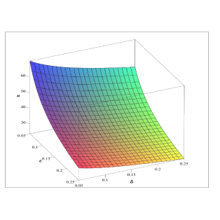
Figure 1: The number of terms to ensure specified accuracy and reliability

Now, for fixed $\varepsilon$ and $\delta$ Figure 2 illustrates the behaviour of the number of terms $n$ as a function of the parameter $p\in[1,2].$ The plot was produced using the values $T=B(0)=\omega=1,$ $\Lambda=3/4,$ and $\varepsilon=\delta=0.1.$

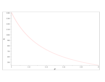
Figure 2: The number of terms as a function of $p$

5 Uniform approximation

Most of stochastic sampling results commonly seen in the literature concern the mean-square convergence, but various practical applications require uniform convergence. To give an adequate description of the performance of sampling approximations in both cases, for points where the processes are relatively smooth and points where spikes occur, one can use the uniform distance instead of the mean-square one. The development of uniform stochastic approximation methods is one of frontiers in applications of stochastic sampling theory to modern functional data analysis.

In this section we present results on uniform truncation error upper bounds appearing in the approximation $\mathbf{X}(t)\approx\mathbf{X}_{n}(t)$ of $Sub_{\varphi}(\Omega)$ and $SSub_{\varphi}(\Omega)$ random processes. We also give some specifications of the general results for which the assumptions can be easily verified.

Let $\mathbf{X}(t),$ $t\in\mathbf{T},$ be a $\varphi$-subgaussian random process. It generates the pseudometrics $\rho_{\mathbf{X}}(t,s)=\tau_{\varphi}(\mathbf{X}(t)-\mathbf{X}(s))$ on $\mathbf{T}.$ Let the pseudometric space $(\mathbf{T},\rho_{\mathbf{X}})$ be separable, $\mathbf{X}$ be a separable process, and $\varepsilon_{0}:=\sup_{t\in\mathbf{T}}\tau_{\varphi}(t)<+\infty.$

Definition 9.

[5] Let $N(v)$ denote the smallest number of elements in an $v$-covering of $\mathbf{T},$ i.e. the smallest number of closed balls $B_{i},$ $i\in I,$ of diameters at most $2v$ and such that $\cup_{i\in I}B_{i}=\mathbf{T}.$ The function $N(v),$ $v>0,$ is called the metric massiveness of the space $\mathbf{T}$ with respect to the pseudometric $\rho_{\mathbf{X}}.$ The function $H(v):=\ln N(v)$ is called the metric entropy of the space $\mathbf{T}$ with respect to the pseudometric $\rho_{\mathbf{X}}.$

Note that the function $N(v)$ coincides with the number of point in a minimal $v$ net covering the space $\mathbf{T}$ and can be equal $+\infty.$

Entropy methods to study the metric massiveness of function calsses and spaces play an important role in modern approximation theory. Various properties and numerous examples of the metric massiveness and the metric entropy can be found in [5, §3.2].

Theorem 5.

[5] Let $r(x),$ $x\geq 1,$ be a non-negative, monotone increasing function such that the function $r\left(e^{x}\right),$ $x\geq 1,$ is convex and

$$I_{r}(v):=\int_{0}^{v}r(N(v))dv<+\infty,$$

where $N(v)$ is the massiveness of the pseudometric space $(\mathbf{T},\rho_{\mathbf{X}}).$

Then, for all $\lambda>0,$ $0<\theta<1,$ it holds

$$\mathbf{E}\exp\left\{\lambda\sup_{t\in\mathbf{T}}|\mathbf{X}(t)|\right\}\leq 2Q(\lambda,\theta)$$ (25)

and

$$\mathbf{P}\left\{\sup_{t\in\mathbf{T}}|\mathbf{X}(t)|\geq u\right\}\leq 2A(\theta,u),$$ (26)

where

$$Q(\lambda,\theta):=\exp\left\{\varphi\left(\frac{\lambda\varepsilon_{0}}{1-\theta}\right)\right\}\,r^{(-1)}\left(\frac{I_{r}(\theta\varepsilon_{0})}{\theta\varepsilon_{0}}\right),$$

$$A(\theta,u):=\exp\left\{-\varphi^{*}\left(\frac{u(1-\theta)}{\varepsilon_{0}}\right)\right\}\,r^{(-1)}\left(\frac{I_{r}(\theta\varepsilon_{0})}{\theta\varepsilon_{0}}\right).$$

Below we give a proof of Theorem 5 which corrects the version with mistakes and the missing proof which appeared in [5, page 107].

Proof.

We will use the following inequality from [5, page 103]

$$\mathbf{E}\exp\left\{\lambda\sup_{t\in\mathbf{T}}|\mathbf{X}(t)|\right\}\leq\prod_{k=1}^{\infty}\left[2N(\theta^{k}\varepsilon_{0})\cdot\exp\left\{\varphi\left(\lambda q_{k}\theta^{k-1}\varepsilon_{0}\right)\right\}\right]^{1/q_{k}},$$

where $(q_{k})_{k=1}^{\infty}$ is a sequence satisfying the inequality $\sum_{k=1}^{\infty}q_{k}^{-1}\leq 1.$

It is easily seen that

$$\mathbf{E}\exp\left\{\lambda\sup_{t\in\mathbf{T}}|\mathbf{X}(t)|\right\}\leq 2^{\sum_{k=1}^{\infty}q_{k}^{-1}}\exp\left\{\sum_{k=1}^{\infty}\frac{H(\theta^{k}\varepsilon_{0})}{q_{k}}+\frac{\varphi\left(\lambda q_{k}\theta^{k-1}\varepsilon_{0}\right)}{q_{k}}\right\},$$

where $H(v)$ is the metric entropy of the pseudometric space $(\mathbf{T},\rho_{\mathbf{X}}).$

Let $q_{k}={1}/{\theta^{k-1}(1-\theta)}.$ Then it follows from the convexity of $r(e^{x})$ that

$$\mathbf{E}\exp\left\{\lambda\sup_{t\in\mathbf{T}}|\mathbf{X}(t)|\right\}\leq 2\exp\left\{\sum_{k=1}^{\infty}\theta^{k-1}(1-\theta)H(\theta^{k}\varepsilon_{0})+\varphi\left(\frac{\lambda\varepsilon_{0}}{1-\theta}\right)\sum_{k=1}^{\infty}\theta^{k-1}(1-\theta)\right\}$$

$$=2\exp\left\{\varphi\left(\frac{\lambda\varepsilon_{0}}{1-\theta}\right)\right\}\cdot r^{(-1)}\left(r\left(\exp\left\{\sum_{k=1}^{\infty}\theta^{k-1}(1-\theta)H(\theta^{k}\varepsilon_{0})\right\}\right)\right)$$

$$\leq 2\exp\left\{\varphi\left(\frac{\lambda\varepsilon_{0}}{1-\theta}\right)\right\}\cdot r^{(-1)}\left(\sum_{k=1}^{\infty}\theta^{k-1}(1-\theta)\cdot r\left(N(\theta^{k}\varepsilon_{0})\right)\right).$$

From the estimate

$$r\left(N(\theta^{k}\varepsilon_{0})\right)\leq\frac{1}{\varepsilon_{0}\theta^{k}(1-\theta)}\int_{\theta^{k+1}\varepsilon_{0}}^{\theta^{k}\varepsilon_{0}}r(N(v))dv$$

we deduce that

$$\sum_{k=1}^{\infty}\theta^{k-1}(1-\theta)\cdot r\left(N(\theta^{k}\varepsilon_{0})\right)\leq\frac{1}{\theta\varepsilon_{0}}\int_{0}^{\theta\varepsilon_{0}}r(N(v))dv.$$

The above estimates imply the inequality (25).

To prove the inequality (26) we note that by (25) for all $\lambda>0$

$$\mathbf{P}\left\{\sup_{t\in\mathbf{T}}|\mathbf{X}(t)|\geq u\right\} \leq \frac{\mathbf{E}\exp\left\{\lambda\sup_{t\in\mathbf{T}}|\mathbf{X}(t)|\right\}}{\exp(\lambda u)}\leq 2\,r^{(-1)}\left(\frac{I_{r}(\theta\varepsilon_{0})}{\theta\varepsilon_{0}}\right)$$

$$\times \exp\left\{-\lambda u+\varphi\left(\frac{\lambda\varepsilon_{0}}{1-\theta}\right)\right\}.$$

By the definition of the Young-Fenchel transform we get

$$\inf_{\lambda\geq 0}\left(-\lambda u+\varphi\left(\frac{\lambda\varepsilon_{0}}{1-\theta}\right)\right)=-\sup_{\lambda\geq 0}\left(\frac{\lambda\varepsilon_{0}}{1-\theta}\cdot\frac{u(1-\theta)}{\varepsilon_{0}}-\varphi\left(\frac{\lambda\varepsilon_{0}}{1-\theta}\right)\right)=-\varphi^{*}\left(\frac{u(1-\theta)}{\varepsilon_{0}}\right).$$

This proves the inequality (26). ∎

Theorem 6.

Let $\mathbf{X}(t),$ $t\in[0,T],$ be a separable $\varphi$-subgaussian random process such that $\sup_{t\in[0,T]}\tau_{\varphi}(t)<+\infty$ and

$$\sup_{|t-s|\leq h}\tau_{\varphi}(\mathbf{X}(t)-\mathbf{X}(s))\leq\sigma(h),$$ (27)

where $\sigma(h),$ $h\geq 0,$ is a monotone increasing continuous function such that $\sigma(0)=0.$ Let $r(\cdot)$ be the function introduced in Theorem 5.

If

$$\tilde{I}_{r}(v):=\int_{0}^{v}r\left(\frac{T}{2\sigma^{(-1)}(u)}+1\right)du<+\infty,$$

then for any $\theta\in(0,1)$ and $\varepsilon>0$

$$\mathbf{P}\left\{\sup_{t\in[0,T]}|\mathbf{X}(t)|\geq\varepsilon\right\}\leq 2\tilde{A}(\theta,\varepsilon),$$

where

$$\tilde{A}(\theta,\varepsilon):=\exp\left\{-\varphi^{*}\left(\frac{\varepsilon(1-\theta)}{\varepsilon_{0}}\right)\right\}\,r^{(-1)}\left(\frac{\tilde{I}_{r}(\theta\varepsilon_{0})}{\theta\varepsilon_{0}}\right).$$

Proof.

Notice that the space $([0,T],\rho_{\mathbf{X}}(t,s))$ is separable. Also, the next inequality holds true

$$N(u)\leq\frac{T}{2\sigma^{(-1)}(u)}+1.$$

Hence, the statement of the theorem follows from Theorem 5. ∎

Remark 2.

In [38] Malliavin derivatives were applied to derive some upper bounds similar to the results in Theorems 5 and 6. However, these bound can not be directly compared with the results in Theorems 5 and 6 as they are valid only for a range of values of $\varepsilon$ which is separated from 0.

Let $\alpha,\gamma\in(1,\infty)$ satisfy $1/\alpha+1/\gamma=1.$

Example 9.

Let $\varphi(x)=|x|^{\alpha}/\alpha,\ 1<\alpha\leq 2.$ Then

$$\tilde{A}(\theta,\varepsilon)=\exp\left\{-\frac{\varepsilon^{\gamma}(1-\theta)^{\gamma}}{\gamma\,\varepsilon_{0}^{\gamma}}\right\}\,r^{(-1)}\left(\frac{\tilde{I}_{r}(\theta\varepsilon_{0})}{\theta\varepsilon_{0}}\right).$$

Example 10.

Let $\sigma(h)=Ch^{\kappa},$ $0<\kappa\leq 1,$ and $r(v)=(v-1)^{\beta},$ $0<\beta<\kappa.$ Then $\sigma^{(-1)}(u)=(u/C)^{1/\kappa},$ $r^{(-1)}(v)=v^{1/\beta}+1,$ and

$$\tilde{I}_{r}(v)=\int_{0}^{v}\left(\frac{C^{1/\kappa}T}{2u^{1/\kappa}}\right)^{\beta}du=\left(\frac{C^{1/\kappa}T}{2}\right)^{\beta}\left(1-\frac{\beta}{\kappa}\right)^{-1}v^{1-\beta/\kappa}.$$

Hence,

$$r^{(-1)}\left(\frac{\tilde{I}_{r}(\theta\varepsilon_{0})}{\theta\varepsilon_{0}}\right)=\frac{C^{1/\kappa}T}{2}\left(1-\frac{\beta}{\kappa}\right)^{-1/\beta}\left(\theta\varepsilon_{0}\right)^{-1/\kappa}+1$$

and

$$\tilde{A}(\theta,\varepsilon)=\exp\left\{-\varphi^{*}\left(\frac{\varepsilon(1-\theta)}{\varepsilon_{0}}\right)\right\}\,\left(\frac{C^{1/\kappa}T}{2}\left(1-\frac{\beta}{\kappa}\right)^{-1/\beta}\left(\theta\varepsilon_{0}\right)^{-1/\kappa}+1\right).$$

If $\beta\to 0,$ then $\left(1-\frac{\beta}{\kappa}\right)^{1/\beta}\to e^{-1/\kappa}$ and we obtain the inequality

$$\tilde{A}(\theta,\varepsilon)\leq\exp\left\{-\varphi^{*}\left(\frac{\varepsilon(1-\theta)}{\varepsilon_{0}}\right)\right\}\,\left(\frac{T}{2}\left(\frac{e\,C}{\theta\varepsilon_{0}}\right)^{1/\kappa}+1\right).$$ (28)

Remark 3.

Note that the particular form of $\sigma(h)$ in Example 10 guarantees Hölder continuity of sample paths of the stochastic process $\mathbf{X}.$ However, Hölder exponents may be different for different functions $\varphi.$

Example 11.

Let $\varphi(x)=|x|^{\alpha}/\alpha,\ 1<\alpha\leq 2,$ $\sigma(h)=Ch^{\kappa},$ $0<\kappa\leq 1,$ and $r(v)=(v-1)^{\beta},$ $0<\beta<\kappa.$ Then, by Examples 9 and 10 it follows that

$$\tilde{A}(\theta,\varepsilon)\leq\exp\left\{-\frac{\varepsilon^{\gamma}(1-\theta)^{\gamma}}{\gamma\,\varepsilon_{0}^{\gamma}}\right\}\,\left(\frac{T}{2}\left(\frac{e\,C}{\theta\varepsilon_{0}}\right)^{1/\kappa}+1\right).$$

Let now $\theta={\varepsilon_{0}}/{\varepsilon}.$ Then for $\varepsilon>\varepsilon_{0}$ we obtain $\theta<1$ and

$$\mathbf{P}\left\{\sup_{t\in[0,T]}|\mathbf{X}(t)|\geq\varepsilon\right\}\leq 2\exp\left\{-\frac{1}{\gamma}\left(\frac{\varepsilon}{\varepsilon_{0}}-1\right)^{\gamma}\right\}\,\left(\frac{T}{2}\left(\frac{e\,\varepsilon\,C}{\varepsilon_{0}^{2}}\right)^{1/\kappa}+1\right).$$

Theorem 7.

Let $\mathbf{X}(t),$ $t\in[0,T],$ be a separable $SSub_{\varphi}(\Omega)$ random process whose spectrum is bandlimited to $[-\Lambda,\Lambda).$ Let the truncated restoration sum $\mathbf{X}_{n}(t)$ for the process $\mathbf{X}(t)$ is given by (3). Then, for any $\theta\in(0,1),$ $\varepsilon>0,$ and such values of $n$ that $z^{*}:=\frac{\omega^{2}T^{2}}{n^{2}\pi^{2}}<1:$

$$\mathbf{P}\left\{\sup_{t\in[0,T]}|\mathbf{X}(t)-\mathbf{X}_{n}(t)|\geq\varepsilon\right\}\leq\exp\left\{-\varphi^{*}\left(\frac{\varepsilon(1-\theta)}{C_{n}}\right)\right\}\,\left(\frac{eTC_{\mathbf{X}}\sqrt{b_{n}}}{2n\theta C_{n}}+1\right),$$

where $C_{\mathbf{X}}$ is the determinative constant of the process $\mathbf{X}(t)$, $b_{n}:=b_{n}(T,T)$ is given by (5) evaluated at $z=z^{*},$

$$C_{n}:=\frac{C_{\mathbf{X}}\mathbf{B}(0)}{n}\cdot\left(\frac{4\omega T}{\pi^{2}(1-z^{*})}+\frac{4\left(z^{*}+1+\frac{1}{n}\right)}{\pi(1-z^{*})^{2}\left(1-\frac{\Lambda}{\omega}\right)}\right)^{2}.$$

Proof.

It follows from (3) and Definition 6 that $\mathbf{Y}_{n}(t)=\mathbf{X}(t)-\mathbf{X}_{n}(t)$ is a $SSub_{\varphi}(\Omega)$ random process with the determinative constant $C_{\mathbf{X}}.$ Hence, by Definition 6 and an application of part 1 of Theorem 1 to $\mathbf{Y}_{n}(t)$ we get

$$\tilde{\varepsilon}_{0}=\sup_{t\in[0,T]}\tau_{\varphi}\left(\mathbf{Y}_{n}(t)\right)\leq C_{\mathbf{X}}\sup_{t\in[0,T]}\left(\mathbf{E}\mathbf{Y}_{n}^{2}(t)\right)^{1/2}\leq\frac{C_{\mathbf{X}}}{n}\sup_{t\in[0,T]}\sqrt{C_{n}(t)}.$$

Notice, that it follows from $n\geq\frac{\omega t}{\pi\sqrt{z}}$ in part 1 of Theorem 1 and (4) that $C_{n}(t)$ is an increasing function of $T$ and $z.$ Therefore,

$$\sup_{t\in[0,T]}{C_{n}(t)}=\mathbf{B}(0)\cdot\sup_{0<z\leq z*}\left(\frac{4\omega T}{\pi^{2}(1-z)}+\frac{4\left(z+1+\frac{1}{n}\right)}{\pi(1-z)^{2}\left(1-\frac{\Lambda}{\omega}\right)}\right)^{2}=\frac{n\,C_{n}}{C_{\mathbf{X}}}$$

and $\tilde{\varepsilon}_{0}\leq C_{n}.$

By Definition 6 and an application of part 2 of Theorem 1 to $\mathbf{Y}_{n}(t)$ we get

$$\sup_{|t-s|\leq h}\tau_{\varphi}(\mathbf{Y}_{n}(t)-\mathbf{Y}_{n}(s))\leq C_{\mathbf{X}}\sup_{|t-s|\leq h}\left(\mathbf{E}\left|\mathbf{Y}_{n}(t)-\mathbf{Y}_{n}(s)\right|^{2}\right)^{1/2}$$

$$\leq C_{\mathbf{X}}\sup_{|t-s|\leq h}\frac{|t-s|}{n}\sqrt{b_{n}(t,s)}.$$

It follows from (5) that $b_{n}(t,s)$ is an increasing function of its arguments $t,s,$ and parameter $z.$ Hence, $\sup_{|t-s|\leq h}b_{n}(t,s)\leq b_{n}(T,T)\leq b_{n}$ and the condition (27) of Theorem 6 is satisfied for the function $\sigma(h)=C_{\mathbf{X}}\sqrt{b_{n}}\cdot h/n.$ Therefore, we can apply the result (28) where $\kappa=1$ and $C=C_{\mathbf{X}}\sqrt{b_{n}}/n.$

Analogously to the proof of Theorem 3 one can show that the upper bound remains valid if the constant $\varepsilon_{0}$ in the expression $\tilde{A}(\theta,\varepsilon)$ is replaced by a larger value. Hence, an application of Theorem 6 to $\mathbf{Y}_{n}(t)$ and the above estimates give

$$\tilde{A}(\theta,\varepsilon)\leq\exp\left\{-\varphi^{*}\left(\frac{\varepsilon(1-\theta)}{C_{n}}\right)\right\}\,\left(\frac{eTC_{\mathbf{X}}\sqrt{b_{n}}}{2n\theta C_{n}}+1\right)$$

which completes the proof. ∎

Corollary 2.

Let $\varphi(x)=|x|^{\alpha}/\alpha,\ 1<\alpha\leq 2,$ in Theorem 7. Then, by Example 11 for $\varepsilon>C_{n}$ it holds

$$\mathbf{P}\left\{\sup_{t\in[0,T]}|\mathbf{X}(t)-\mathbf{X}_{n}(t)|\geq\varepsilon\right\}\leq 2\exp\left\{-\frac{1}{\gamma}\left(\frac{\varepsilon}{C_{n}}-1\right)^{\gamma}\right\}\,\,\left(\frac{\varepsilon eTC_{\mathbf{X}}\sqrt{b_{n}}}{2nC^{2}_{n}}+1\right).$$

It follows from the definition of $C_{n}$ that $C_{n}\sim 1/n,$ when $n\to\infty.$ Hence, for a fixed value of $\varepsilon$ the right-hand side of the above inequality vanishes when $n$ increases.

Similarly to Section 4 one can define the uniform approximation of $\mathbf{X}(t)$ with a given accuracy and reliability.

Definition 10.

$\mathbf{X}_{n}(t)$ uniformly approximates $\mathbf{X}(t)$ with accuracy $\varepsilon>0$ and reliability $1-\delta,$ $0<\delta<1,$ if

$$\mathbf{P}\left\{\sup_{t\in[0,T]}|\mathbf{X}(t)-\mathbf{X}_{n}(t)|>\varepsilon\right\}\leq\delta.$$

By Definition 10 and Theorem 7 we obtain the following result.

Theorem 8.

Let $\mathbf{X}(t),$ $t\in\mathbf{R},$ be a separable $SSub_{\varphi}(\Omega)$ process with a bounded spectrum, $\theta\in(0,1),$ $\varepsilon>0,$ and $n$ is such an positive integer number that $z^{*}:=\frac{\omega^{2}T^{2}}{n^{2}\pi^{2}}<1.$ Then, $\mathbf{X}_{n}(t)$ uniformly approximates $\mathbf{X}(t)$ with accuracy $\varepsilon$ and reliability $1-\delta$ if the following inequality holds true

$$\exp\left\{-\varphi^{*}\left(\frac{\varepsilon(1-\theta)}{C_{n}}\right)\right\}\,\left(\frac{eTC_{\mathbf{X}}\sqrt{b_{n}}}{2n\theta C_{n}}+1\right)\leq\delta.$$

Corollary 3.

Let $\varphi(x)=|x|^{\alpha}/\alpha,\ 1<\alpha\leq 2,$ in Theorem 8. Then, $\mathbf{X}_{n}(t)$ uniformly approximates $\mathbf{X}(t)$ with accuracy $\varepsilon$ and reliability $1-\delta$ if $\varepsilon>C_{n}$ and

$$\exp\left\{-\frac{1}{\gamma}\left(\frac{\varepsilon}{C_{n}}-1\right)^{\gamma}\right\}\,\,\left(\frac{\varepsilon eTC_{\mathbf{X}}\sqrt{b_{n}}}{2nC^{2}_{n}}+1\right)<\delta/2.$$

Notice that for Gaussian processes $\mathbf{X}(t)$ all results of this section hold true when $\alpha=\gamma=2$ and $C_{\mathbf{X}}=1.$

6 Conclusions

These results may have various applications for the approximation of stochastic processes. The obtained rate of convergence provides a constructive algorithm for determining the number of terms in the WKS expansions to ensure the approximation of $\varphi$-sub-Gaussian processes with given accuracy and reliability. The developed methodology and new estimates are important extensions of the known results in the stochastic sampling theory to the space $L_{p}([0,T])$ and the class of $\varphi$-sub-Gaussian random processes. In addition to classical applications of $\varphi$-sub-Gaussian random processes in signal processing, the results can also be used in new areas, for example, compressed sensing and actuarial modelling, see, e.g., [18, 39, 40].

It would be of interest

• to apply this methodology to other WKS sampling problems, for example, shifted sampling, irregular sampling, aliasing errors, see [30, 31, 32] and references therein;

• to derive analogous results for the multidimensional case and random fields;

• to derive similar results for the sub-Gaussian case by the generic chaining method and to compare them with the obtained bounds.

References

Belyaev [1959] Yu.K. Belyaev, Analytical random processes, Theory Probab. Appl. 4(4) (1959) 402–409.
Biermé, Lacaux [2014] H. Biermé, C. Lacaux, Modulus of continuity of some conditionally sub-Gaussian fields, application to stable random fields, Bernoulli. 21(3) (2015) 1719–1759.
Borell [1977] C. Borell, Tail probabilities in Gauss space, in: Vector Space Measures and applications, Dublin, 1977, in: Lecture Notes in Math., vol. 644, Springer, 1978, pp. 71-82.
Butzer et al. [2011] P.L. Butzer, P.J.S.G. Ferreira, J.R. Higgins, G. Schmeisser, R.L. Stens, The sampling theorem, Poisson’s summation formula, general Parseval formula, reproducing kernel formula and the Paley-Wiener theorem for bandlimited signals – their interconnections, Appl. Anal. 90(3-4) (2011) 431–461.
Buldygin, Kozachenko [2000] V.V. Buldygin, Yu.V. Kozachenko, Metric Characterization of Random Variables and Random Processes, American Mathematical Society, Providence R.I., 2000.
Cambanis, Masry [1982] S. Cambanis, E. Masry, Truncation error bounds for the cardinal sampling expasnion of band - limited signals, IEEE Trans. Inform. Theory. IT-28/4 (1982) 605–612.
Chen, Ramabadran [1994] K. Chen, T.V. Ramabadran, Near-lossless compression of medical images through entropy-coded DPCM, IEEE Trans. Med. Imaging. 13(3) (1994) 538–548.
Csáki, Csörgő [1992] E. Csáki, M. Csörgő, Inequalities for increments of stochastic processes and moduli of continuity,
Ann. Probab. 20(2) (1992) 1031–1052.
Dudley [1967] R. M. Dudley, The sizes of compact subsets of Hilbert space and continuity of Gaussian processes, J. Funct. Anal. 1
(1967) 290–330.
Dudley [1999] R. M. Dudley, Uniform central limit theorems, Cambridge University Press, Cambridge, 1999.
Giuliano Antonini et al. [2003] R. Giuliano Antonini, Yu.V. Kozachenko,
T. Nikitina, Spaces of -sub-Gaussian random
variables, Mem. Mat. Appl. 121(27) fasc 1 (2003) 95–124.
Giuliano Antonini et al. [2013] R. Giuliano Antonini, T.-Ch. Hu, Yu. Kozachenko, A. Volodin, An application of -subgaussian technique to Fourier analysis, J. Math. Anal. Appl. 408(1) (2013) 114–124.
Fernique [1975] X. Fernique, Régularité des trajectoires des fonctions aléatoires gaussiennes, in: Ecole d’Eté de Probabilités de
Saint-Flour IV-1974, in: Lecture Notes in Math., vol. 480, Springer, 1975, pp. 1–96.
Ferrando, Pyke [2008] S.E. Ferrando, R. Pyke, Ideal denoising for signals in sub-Gaussian noise, Appl. Comput. Harmon. Anal. 24(1) (2008) 1–13.
Hartenstein, Saupe [1998] H. Hartenstein, D. Saupe, On entropy minimization for near-lossless differential coding, IEEE Commun. Lett. 2(4) (1998) 97–99.
He, Song [2011] G. He, Z. Song, Approximation of WKS sampling theorem on random signals, Numer. Funct. Anal. Optim. 32(4) (2011) 397–408.
Higgins et al. [2000] J.R. Higgins, G. Schmeisser, J.J. Voss, The sampling theorem and several equivalent results in analysis, J. Comp. Anal. Appl. 2 (2000) 333–371.
Hogan, Lakey [2012] J.A. Hogan, J.D. Lakey, Duration and Bandwidth Limiting. Prolate Functions, Sampling, and Applications, Birkhäuser/Springer, New York, 2012.
Kahane [1960] J.P. Kahane, Propriétés locales des fonctions à séries de Fourier aléatoires, Studia Math. 19(1) (1960) 1–25.
Kozachenko, Kamenshchikova [2009] Yu. Kozachenko, O. Kamenshchikova, Approximation of stochastic processes in the space , Theor. Probab. Math. Statist. 79 (2009) 83–88.
Kozachenko, Kovalchuk [1998] Yu. Kozachenko, Yu. Kovalchuk,
Boundary value problems with random initial conditions and
functional series from I. Ukrainian
Math. J. 50 (1998) 504–515.
Kozachenko et al. [2013] Yu. Kozachenko, A. Olenko, O. Polosmak, On convergence of general wavelet decompositions of nonstationary stochastic processes, Electron. J. Probab. 18(69) (2013) 1–21.
Kozachenko et al. [2014] Yu. Kozachenko, A. Olenko, O. Polosmak, Uniform convergence of compactly supported wavelet expansions of Gaussian random processes, Comm. Statist. Theory Methods. 43(10-12) (2014) 2549–2562.
Kozachenko, Ostrovskyi [1985] Yu. Kozachenko, E. Ostrovskyi, Banach spaces of random variables of Sub-gaussian type, Theor. Probab. Math. Statist. 32 (1985) 42–53.
Kozachenko et al. [2005] Yu. Kozachenko, O. Vasylyk, R. Yamnenko, Upper estimate of overrunning by random process the level specified by continuous function, Random Oper. Stoch. Equ. 13(2) (2005) 111–128.
Krasnosel’skii, Rutickii [1961] M.A. Krasnosel’skii, Ya.B. Rutickii, Convex Functions and Orlicz Spaces, Noordhof, Gröningen, 1961.
Ledoux [1996] M. Ledoux, Isoperimetry and Gaussian analysis, in: Lectures on Probability Theory and Statistics, Saint-Flour, 1994, in: Lecture Notes in Math., vol. 1648, Springer, 1996, pp. 165–294.
Ledoux, Talagrand [1991] M. Ledoux, M. Talagrand, Probability in Banach spaces. Isoperimetry and processes, Springer-Verlag, Berlin, 1991.
Moen et al. [2013] K. Moen, H. Šikić, G. Weiss, E. Wilson, A panorama of sampling theory, in Excursions in harmonic analysis, Vol. 1, Birkhäuser/Springer, New York, 2013, pp. 107–127.
Olenko, Pogány [2005] A. Olenko, T. Pogány, A precise upper bound for the error of interpolation of stochastic processes, Theor. Probab. Math. Statist. 71 (2005) 151–163.
Olenko, Pogány [2006] A. Olenko, T. Pogány, Time shifted aliasing error upper bounds for truncated sampling cardinal series, J. Math. Anal. Appl. 324(1) (2006) 262–280.
Olenko, Pogány [2011] A. Olenko, T. Pogány, Average Sampling Restoration of Harmonizable Processes. Comm. Statist. Theory Methods. 40(19-20) (2011) 3587–3598.
Piranashvili [1967] Z.A. Piranashvili, On the problem of interpolation of random processes, Theory Probab. Appl. 12(4) (1967) 647–657.
Pogány [1999] T. Pogány, Almost sure sampling restoration of bandlimited stochastic signals, in Higgins J.R., Stens, R.L. (Eds.) Sampling Theory in Fourier and Signal Analysis: Advanced Topics, Oxford University Press, Oxford, 1999, pp. 203–232, 284–286.
Smale, Zhou [1999] S. Smale, D.-X. Zhou, Shannon sampling. II. Connections to learning theory, Appl. Comput. Harmon. Anal. 19(3) (2005) 285–302.
Talagrand [2005] M. Talagrand, The generic chaining. Upper and lower bounds of stochastic processes, Springer-Verlag, Berlin, 2005.
Talagrand [2014] M. Talagrand, Upper and lower bounds for stochastic processes. Modern methods and classical problems, Springer, Heidelberg, 2014.
Viens, Vizcarra [2007] F.G. Viens, A.B. Vizcarra,
Supremum concentration inequality and modulus of continuity for sub-nth chaos processes,
J. Funct. Anal. 248(1) (2007) 1–26.
Xue, Zou [2011] L. Xue, H. Zou, Sure independence screening and compressed random sensing, Biometrika. 98 (2011) 371–380.
Yamnenko [2006] R. Yamnenko, Ruin probability for generalized -sub-Gaussian fractional Brownian motion, Theory Stoch. Process. 12(3-4) (2006) 261–275.
Zayed, Schmeisser [2014] A.I. Zayed, G. Schmeisser, (Eds.) New Perspectives on Approximation and Sampling Theory.
Festschrift in Honor of Paul Butzer’s 85th Birthday, Birkhäuser/Springer, New York, 2014.