Orbital evolution and search for eccentricity and apsidal motion in the eclipsing HMXB 4U 1700–37

Abstract

In the absence of detectable pulsations in the eclipsing High Mass X-ray binary 4U 1700–37, the orbital period decay is necessarily determined from the eclipse timing measurements. We have used the earlier reported mid-eclipse time measurements of 4U 1700–37 together with the new measurements from long term light curves obtained with the all sky monitors RXTE–ASM, Swift–BAT and MAXI–GSC, as well as observations with RXTE–PCA, to measure the long term orbital evolution of the binary. The orbital period decay rate of the system is estimated to be ${\dot{P}}/P=-(4.7\pm 1.9)\times 10^{-7}$ yr^-1, smaller compared to its previous estimates. We have also used the mid-eclipse times and the eclipse duration measurements obtained from 10 years long X-ray light-curve with Swift–BAT to separately put constraints on the eccentricity of the binary system and attempted to measure any apsidal motion. For an apsidal motion rate greater than 5 degrees per year, the eccentricity is found to be less than 0.008, which limits our ability to determine the apsidal motion rate from the current data. We discuss the discrepancy of the current limit of eccentricity with the earlier reported values from radial velocity measurements of the companion star.

1 Introduction

1.1 Orbital evolution and apsidal motion in X-ray binaries

The orbits of X-ray binaries evolve due to various mechanisms like mass and angular momentum exchange between the compact object and the companion star, tidal interaction between the binary components (Lecar, Wheeler & McKee, 1976; Zahn, 1977), magnetic braking (Rappaport, Verbunt & Joss, 1983), stellar wind driven angular momentum loss (Brookshaw & Tavani, 1993; van den Heuvel, 1994), X-ray irradiated wind outflow (Ruderman et al., 1989) and gravitational wave radiation (Verbunt, 1993). In addition to orbital period evolution, the elliptic orbits of X-ray binaries also undergo apsidal motion. The classical apsidal motion is caused by tidal force (Cowling, 1938; Sterne, 1939) and hence the rate of apsidal angle change is directly related to the stellar structure constant of the component stars (Kopal, 1978; Claret & Gimenez, 1993). For an accreting X-ray pulsar, repeated measurements of orbital parameters by pulse timing analysis at separate intervals of time is an efficient way to study the orbital evolution of the binary system (Cen X–3 – Kelley et al. 1983; Her X–1 – Staubert, Klochkov & Wilms 2009; SMC X–1 – Levine et al. 1993; LMC X–4 – Levine, Rappaport & Zojcheski 2000; Naik & Paul 2004; 4U 1538–52 – Mukherjee et al. 2006; SAX J1808.4–3658 – Jain, Dutta & Paul 2008; OAO 1657–415 – Jenke et al. 2012) as well as its rate of apsidal motion (4U 0115+63 – Raichur & Paul 2010a). For eclipsing HMXB pulsars like Vela X–1 (Deeter et al., 1987) and 4U 1538–52 (Falanga et al., 2015), the rate of apsidal motion can also be calculated from the offset in the local eclipse period and the mean sidereal period, which is determined from pulse timing analysis. In case of eclipsing X-ray binaries, eclipse timing technique is used to determine the orbital evolution of binary systems (EXO 0748–676 – Parmar et al. 1991; Wolff et al. 2009; 4U 1822–37 – Jain, Paul & Dutta 2010; XTE J1710–281 – Jain & Paul 2011) as well as estimating parameters of the companion star and masses of the compact object (Coley, Corbet & Krimm, 2015; Falanga et al., 2015). In eclipse timing technique, the mid-eclipse times are used as fiducial markers to study any change in orbital period of the binary system. Mid-eclipse timing measurements have also been used to determine the rate of apsidal motion and other orbital parameters in case of eccentric optical eclipsing binaries (Gimenez & Garcia-Pelayo, 1983; Wolf et al., 2004; Zasche et al., 2014). In the absence of pulsations or eclipses, stable orbital modulation curves have also been found useful for measurements of orbital evolution of some X-ray binaries like Cyg X–3 (Singh et al., 2002) and 4U 1820–30 (Peuten et al., 2014).

Orbital decay of the compact HMXBs are also of interest in the context of short GRBs and gravitational wave astronomy as these are the progenitors of double compact binaries. The massive companion will leave behind a second compact star and if the two compact stars survive as a double compact binary, eventual merging of the two stellar components are believed to produce the short GRBs and are also expected to produce the sources for gravitational wave detection (Belczynski, Kalogera & Bulik, 2002; Abadie et al., 2010).

1.2 4U 1700–37

The massive X-ray binary 4U 1700–37 was discovered with Uhuru (Jones et al., 1973), which revealed it to be an eclipsing binary system with an orbital period of 3.412 days. The optical companion, HD 153919, is a O6.5 Iaf+ star, situated at a distance of 1.9 kpc and one of the most massive and hottest stars known in an HMXB (Ankay et al., 2001). The nature of the compact object is uncertain due to lack of X-ray pulsations from the system (Rubin et al., 1996). Lack of pulsations from 4U 1700–37 makes it difficult to determine the parameters of the binary orbit, especially eccentricity of the orbit and hence the rate of apsidal motion. Estimation of the orbital parameters using radial velocity measurements of the companion star HD 153919 from the ultraviolet and optical spectral lines (Hutchings, 1974; Heap & Corcoran, 1992; Clark et al., 2002; Hammerschlag-Hensberge, van Kerkwijk & Kaper, 2003) was complex due to extreme mass loss rate of the companion as well as very high stellar wind. Previous measurements of orbital parameters by Hammerschlag-Hensberge, van Kerkwijk & Kaper (2003) using ultraviolet spectral lines with International Ultraviolet Explorer, found it to satisfy an orbital solution with an eccentricity e $\sim$ 0.22. 4U 1700–37 is an archetypal system to study the orbital evolution using eclipse timing as it is a bright source with sharp eclipse transitions in the hard X-rays.

Earlier measurements of the mid-eclipse times spanning 20 years, both from the single pointed observations covering one full orbital cycle from Uhuru (Jones et al., 1973), Copernicus (Branduardi, Mason & Sanford, 1978) and EXOSAT (Haberl, White & Kallman, 1989) as well as continuous observations with the all sky monitors Granat/WATCH (Sazonov et al., 1993) and BATSE (Rubin et al., 1996), showed an orbital period decay rate of ${\dot{P}}/P=-3\times 10^{-6}$ yr^-1 (Rubin et al., 1996). Recent work by Falanga et al. (2015), using the mid-eclipse measurements from RXTE–ASM and INTEGRAL, along with the previous mid-eclipse measurements from Rubin et al. (1996), showed a slower orbital decay with a rate of ${\dot{P}}/P=-1.6\times 10^{-6}$ yr^-1.

In this work, we have used the above mentioned mid-eclipse times and the new mid-eclipse time measurements to obtain a long term eclipse history and orbital evolution of the system. We then investigated the possibility of estimating or constraining the eccentricity and the rate of apsidal motion of 4U 1700–37 using the mid-eclipse timing measurements and the eclipse duration measurements independently with 10 years of Swift–BAT light curves.

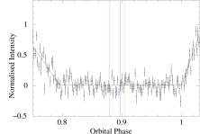
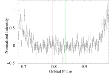
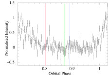
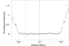
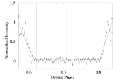
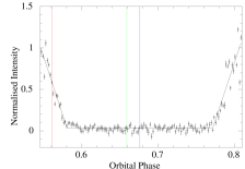
Figure 1: Orbital intensity profile near the eclipse constructed for 3 light curve segments for 5-12 keV RXTE–ASM (top panel), 3 light curve segments for 15-50 keV Swift–BAT (middle panel) and 5-20 keV MAXI–GSC light curve (bottom panel). Blue line denotes the measured mid-eclipse phase, red line denotes the mid-eclipse phase expected from an orbital period change of ${\dot{P}}/P=-3.3\times 10^{-6}$ yr^-1 from Rubin et al. (1996) and green line is the expected mid-eclipse phase from an orbital period change of ${\dot{P}}/P=-1.6\times 10^{-6}$ yr^-1 from Falanga et al. (2015).

2 Orbital Period Evolution

2.1 Mid-eclipse time measurements

We have used the earlier reported mid-eclipse measurements from single pointed observations covering the X-ray eclipse with Uhuru (Jones et al., 1973), Copernicus (Branduardi, Mason & Sanford, 1978) and EXOSAT (Haberl, White & Kallman, 1989). We have also used the mid-eclipse time from a Copernicus observation in 1974 (Mason, Branduardi & Sanford, 1976) which was not used in the previous studies because it showed higher residuals in the linear fit to the mid-eclipse times (Rubin et al., 1996; Falanga et al., 2015). However, as it will be shown later in Figure 3, this datapoint is less than 2 $\sigma$ different from the quadratic fit and is not an outlier anymore (blue datapoint in Figure 3). Mid-eclipse times were also reported from the long term observations with X-ray all sky monitors Granat/WATCH (Sazonov et al., 1993), BATSE (Rubin et al., 1996) and INTEGRAL (Falanga et al., 2015), which are also used in the present analysis.

We have used long term light curves from RXTE–ASM (Levine et al., 1996), Swift–BAT Transient Monitor (Krimm et al., 2013) and MAXI–GSC (Matsuoka et al., 2009) to determine new mid-eclipse times of 4U 1700–37. Falanga et al. (2015) had also reported mid-eclipse times from RXTE–ASM lightcurves in the energy band of 1.5–12 keV. However, as seen in Figure 2 in Falanga et al. (2015), the eclipse is sharper and more pronounced in the light-curve of RXTE–ASM in 5–12 keV energy band compared to its profile seen in 1.3–3 keV and 3–5 keV energy band. This is due to photo-electric absorption of X-rays by the dense stellar wind of the companion which affects the soft X-rays photons more than the hard X-rays photons (van der Meer et al., 2007). Therefore, we have used 16 years long 5–12 keV light curve with RXTE–ASM in this work and divided it into 3 segments, each consisting of about 5 years of data. The 10 years of Swift–BAT light curve in the 15-50 keV energy band was divided into 3 segments, each of duration 3.3 years. The MAXI–GSC light curve for 4.5 years was extracted in 5-20 keV energy band using the MAXI on demand data processing. We have applied barycentric corrections to the light-curves using the FTOOLS task ‘earth2sun’. Eclipses are barely identifiable in only few segments of Swift–BAT light-curves, which has the highest sensitivity amongst the three X-ray all sky monitors in hard X-rays utilized here. In addition, the instruments have very sparse and uneven sampling making it impossible to measure the mid-eclipse times from unfolded light-curves which requires both ingress and egress to be sampled adequately, necessitating folding of light-curves. The orbital period of the system is estimated separately for each segments of light curves using the FTOOLS task ‘efsearch’ and then these light-curves are folded with their respective orbital period with the FTOOLS task ‘efold’ to create orbital intensity profiles. The orbital intensity profiles near the eclipse were fitted with two ramp function having different linear ingress and egress profiles and a constant count-rate during the eclipse, given in Equation  1

$$F(X) = P3\quad\mathrm{for}\quad(P1-P2)<X<(P1+P2)$$ (1)

$$= P4\times(X-(P1+P2))+P3\quad\mathrm{for}\quad X>(P1+P2)$$

$$= -P5\times(X-(P1-P2))+P3$$

$$\mathrm{for}\quad X<(P1-P2)$$

where P1 is the mid-eclipse phase, P2 is the half width of the eclipse, P3 is the count-rate during eclipse, P4 is the slope during eclipse egress, P5 is the slope during eclipse ingress. The fitting of the function is done in the orbital phase range of about $\pm$ 0.15 around the mid-eclipse phase. The orbital intensity profile outside the eclipses have not been used for fitting with the double ramp function as it is energy dependent and has presence of flares outside eclipse as seen in the top panels of Figure 2. The inverse of the slope of the eclipse ingress and eclipse egress are an approximate measure of the ingress and egress durations. The ingress durations obtained from the three RXTE–ASM profiles, three Swift–BAT profiles and the MAXI–GSC profiles are 0.08, 0.1, 0.14, 0.04, 0.05, 0.04, 0.07 of the orbital period while the egress durations are 0.04, 0.04, 0.04, 0.03, 0.04, 0.04, 0.06 respectively. There is better overall agreement between the eclipse egress durations compared to the ingress durations, the latter seems to be larger in the RXTE–ASM and MAXI–GSC data. This is in agreement with additional absorption before the eclipse due to the presence of an accretion wake (Coley, Corbet & Krimm, 2015), effect of which is more prominent in the ASM energy band. However, for the main purpose of this paper, we require the mid-eclipse time and duration of the total eclipse. By using the double ramp function given in Equation  1, these two quantities are measured independent of the ingress and egress durations and their variation or energy dependence.
We have also used RXTE–PCA observations (ObsId 30094), from April 1999 to August 1999, covering eclipse ingress and egress for 120 days or 11 orbital cycles. The light-curve of RXTE–PCA observations is folded with the orbital period estimated for the first segment of RXTE–ASM light curve.

Figure 1 shows the orbital intensity profiles near the eclipses created from 3 light-curve segments of RXTE–ASM, 3 light-curve segments of Swift–BAT and the MAXI–GSC light-curve, fitted with a two ramp function. The blue vertical line in each panel denotes the measured mid-eclipse phase, red line denotes the mid-eclipse phase expected from the orbital period decay extrapolated from Rubin et al. (1996) and the green line is the expected mid-eclipse phase from the orbital period decay extrapolated from Falanga et al. (2015). All the mid-eclipse times extrapolated from Rubin et al. (1996) and all but one from Falanga et al. (2015) appear before the measured mid-eclipse phase for all the orbital intensity profiles, implying that the orbital period decay is lower than the previously estimated values.

The mid-eclipse times used for the analysis, both the earlier reported values as well as the new mid-eclipse times, are given in Table 1. The previously quoted uncertainities on the mid-eclipse times from Uhuru, Copernicus and EXOSAT were re-estimated by Rubin et al. (1996) and were calculated disparately from that of the mid-eclipse times from Granat/Watch and BATSE observations given in Table 2 in Rubin et al. (1996). The different error bars quoted previously are only the statistical errors. However, eclipse measurements in different energy bands with different instruments are also likely to have some systematic differences. To have a more realistic estimates of error bars and only with the aim of measuring a long term period derivative, we have re-estimated the errors on the mid-eclipse times, which are now likely to include the systematic differences between the different instruments. We have divided the mid-eclipse times into two segments, from MJD: 41452 - 49150 and MJD: 49151 - 56468. A linear fit is done separately on these two segments and the average standard deviation of the data-points from the linear fit is taken as the errors on the mid-eclipse times for these two segments (given in Table 1).

Figure 2: Top panel: Plot of the orbital intensity profile created out of 10 years of Swift–BAT data in 15-50 keV energy band (left panel) and 16 years of RXTE–ASM in 5-12 keV energy band (right panel), which shows an averaged smooth profile with sharp eclipse. Bottom panel: Plot of the folded orbital intensity profile near the eclipse using RXTE–PCA (red line) observations overlaid on the EXOSAT–GSPC orbital profile (black line), which shows the presence of flares and dips just outside the eclipse.

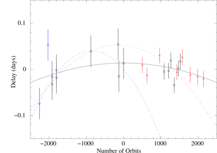
Figure 3: Delay in mid-eclipse times with respect to a constant orbital period. The black circles are the archival measurements of the mid-eclipse times and the red triangles are the new measurements of mid-eclipse times. The blue box datapoint is the mid-eclipse time measurement from Copernicus 1974 observation, which was not used in previous studies on the orbital evolution of the system but is used in this study. The errors on the mid-eclipse times are re-calculated as mentioned in Section 2.1. The solid black line is the quadratic component of the best fits to the mid-eclipse times. The blue dashed line and the magenta dot-dashed line are the quadratic components of the best-fits reported in Rubin et al. (1996) and Falanga et al. (2015) respectively.

2.2 Systematic errors associated with the mid-eclipse time measurement with EXOSAT–GSPC and RXTE–PCA

As seen in top panel of Figure 2, the orbital intensity profile of 4U 1700–37 constructed out of long term light curves from the X-ray all sky monitors like Swift–BAT show a smooth profile with a sharp eclipse due to averaging effects of observations made over many orbits. However at short timescales, the light curves show strong variations, including flares and dips, characteristic of many HMXBs. Among the light curves of 4U 1700–37, those with single observation covering eclipse like EXOSAT–GSPC and RXTE–PCA show strong flares and dips (bottom panel of Figure 2), which introduces significant uncertainities in the eclipse ingress and egress profiles and hence, in the mid-eclipse time determination. The mid-eclipse time estimated from the EXOSAT observation in 1985 was quoted a statistical error of 0.003 days (Haberl, White & Kallman, 1989). We have extracted the EXOSAT–GSPC light curve in the 8–14 keV band and constructed the orbital intensity profile by folding it with the orbital period mentioned in Haberl, White & Kallman (1989). As seen in the right panel of Figure 2, the determination of the exact point of ingress and egress of the eclipse is complicated by the presence of flares and/or dips around the eclipse ingress and egress. To further emphasize on the contribution of flares in uncertainities on the mid-eclipse times in case of pointed observations, we have overlaid the orbital intensity profile from the RXTE–PCA observations (ObsId:30094) in the same plot. From the right panel of Figure 2, we infer that the statistical error of 0.003 days or 260 secs quoted in Haberl, White & Kallman (1989) is an underestimate of the actual error on the mid-eclipse time, as there is a larger systematic error owing to flares/dips. Determination of eclipse duration is also complicated by the presence of same flares and/or dips. In fact the eclipse durations determined from single observations with Uhuru (Jones et al., 1973), Copernicus (Branduardi, Mason & Sanford, 1978) and EXOSAT (Haberl, White & Kallman, 1989) are considerably larger with large error bars than those estimated from long term light curves from the all sky monitors.

We have re-calculated the errors on the EXOSAT mid-eclipse time as mentioned in Section 2.1. It appears that the faster rate of orbital period decay in the earlier estimates (Rubin et al., 1996; Falanga et al., 2015) were result of small statistical error considered for the EXOSAT mid-eclipse data.

2.3 Orbital evolution of 4U 1700–37

The mid-eclipse times given in Table 1 along with their errors are fitted to a quadratic function

$$T_{N}=T_{0}+PN+\frac{1}{2}P{\dot{P}}N^{2}$$ (2)

where $T_{N}$ is the mid-eclipse time of the N^th orbital cycle. P is the orbital period in days and ${\dot{P}}$ is the orbital period derivative, both at time $\mathrm{T_{0}}$.

The definition of $\mathrm{T_{0}}$ and orbit number are same as mentioned in Rubin et al. (1996). The best fit to the mid-eclipse times for a constant orbital period gives $\mathrm{T_{0}}=49149.412\pm 0.006$ MJD, orbital period P = 3.411660 $\pm$ 0.000004 days with a $\chi^{2}=28.3$ for 22 degrees of freedom. The mid-eclipse times fitted with a quadratic function as in Equation 2 gives the values of orbital period decay ${\dot{P}}/P=-(4.7\pm 1.9)\times 10^{-7}$ yr^-1 with a $\chi^{2}=23.8$ for 21 degrees of freedom. The orbital ephemeris is also tabulated in Table 2. For the orbital ephemeris given in Falanga et al. (2015), the value of $\chi^{2}=67.15$ for 24 degrees of freedom. The orbital period decay rate of 4U 1700–37 determined here is smaller compared to the earlier estimates (Haberl, White & Kallman, 1989; Rubin et al., 1996; Falanga et al., 2015). A plot of the delay in mid-eclipse times with respect to a constant orbital period as a function of the number of orbital cycles, along with the best fit quadratic function is given in Figure 3. The quadratic function reported in Rubin et al. (1996) and Falanga et al. (2015) are overlaid on the same plot.

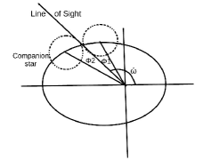
Figure 4: The ellipse represents the motion of the companion star with respect to the compact star at the focus. See text for description of the various angles.

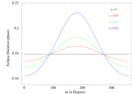
Figure 5: Plot of variation of eclipse duration as a function of $\omega^{{}^{\prime}}$ for different value of eccentricity, for an orbital inclination of 66^∘. Increasing values of eccentricity increases the ratio of maximum to minimum eclipse duration.

3 Eccentricity and Apsidal Motion of 4U 1700–37

In a close binary stellar system, the rate of apsidal motion due to tidal forces is given by (Claret & Gimenez, 1993)

$$\frac{\dot{\omega}}{360}=k(\frac{R_{\star}}{a})^{5}(15qg(e)+\Omega^{2}(1+q)f(e))\quad\mathrm{deg/cycle}\\$$ (3)

where e is the eccentricity, R_⋆ is the companion star radius, a is the binary separation, q is the mass ratio of the compact object to the companion star and $\Omega$ is ratio of the rotational velocity of the companion star to its orbital angular velocity

$$g(e)=(1+\frac{3}{2}e^{2}+\frac{1}{8}e^{4})(1-e^{2})^{-5}$$

$$f(e)=(1-e^{2})^{-2}$$

Using the binary parameters of 4U 1700–37 along with its uncertainities (R_⋆, a, q, P_orb from Table 3), a reasonable value of stellar constant log k of $-2.2$ corresponding to the companion star HD 153919 type (Claret, 2004) and e in the range of 0.01–0.22, we get an apsidal motion rate of $10\pm 3$ degrees/year. For Vela X–1 and 4U 1538–522, using the binary parameters from Table 7 in Falanga et al. (2015), an estimation of the rate of apsidal motion is $\sim$ 1 degree/yr and 5 degree/yr respectively, similar to that measured in these sources (Deeter et al., 1987; Falanga et al., 2015). The major source of uncertainity in estimating the rate of apsidal motion arises from the value of stellar constant k, which for some HMXBs are constrained by observations of apsidal motion in X-ray binaries (Raichur & Paul, 2010b).

The two interesting consequences of a large apsidal advance rate in an eclipsing X-ray binary are that the delay in the mid-eclipse times and the value of eclipse duration both would vary with a period of 360${}^{\circ}/\dot{\omega}$. The delay in mid-eclipse times due to apsidal motion is seen in close eclipsing optical binary stars (Gimenez & Garcia-Pelayo, 1983; Wolf et al., 2004; Zasche et al., 2014). The mid-eclipse times (Table 1) and the corresponding eclipse duration measurements of 4U 1700–37 have been carried out with a large number of instruments of different sensitivities and in different energy bands. We have mentioned before that this causes significant systematic differences and therefore are not ideal to investigate the effects of apsidal motion. Eclipse duration is also found to be dependent on the energies of the X-rays with some eclipses lasting longer at lower energies than higher energies (van der Meer et al., 2007). So we have used hard X-ray light curve from Swift-BAT which has the highest statistical quality (second panel in Figure 1) and have divided it into 10 segments of 1 year data and searched for the signatures of an apsidal motion for an eccentric orbit. The yearly measurements of the eclipse data (mid-eclipse time and eclipse duration) are useful to probe an $\dot{\omega}$ in the range of 5-200 degrees per year. Since these 10 measurements are from the data obtained with the same instrument, it is unlikely to have much systematic difference between different data points.

3.1 Mid-eclipse time variation due to apsidal motion

For a system having a small eccentricity and undergoing an apsidal motion, the mid-eclipse times show a sinusoidal pattern given by the following Equation (Gimenez & Garcia-Pelayo, 1983)

$$T_{N}-(T_{0}+PN)=\frac{eP_{a}}{\pi}\mathrm{cos}(\omega_{0}+\Delta\omega N)$$ (4)

where $\Delta\omega$ is the change in $\omega$ in one orbital cycle. P_a is the anomalistic orbital period defined by the interval of time between two consecutive periastron passages and given by :

$$P_{a}=\frac{P}{(1-\frac{\Delta\omega}{2\pi})}$$

For moderate values of $\Delta\omega$, P${}_{a}\sim$ P (orbital period).

The orbital inclination of the binary system 4U 1700–37 is of the order of 60^∘–70^∘ (Rubin et al., 1996; Falanga et al., 2015) and will lead to a change in the estimation of $\omega_{0}$ of the system. However, the estimation of $\Delta\omega$ and eccentricity e is independent of the orbital inclination of the system.

3.2 Variation in eclipse duration due to apsidal motion

By considering the motion of the companion star around the compact object, we initially calculated the eclipse durations as a function of the angle of periastron for different values of e for an orbital inclination of 90^∘. In Figure 4, the ellipse represents the motion of the companion star with respect to the compact star at the centre. $\phi_{1}$ and $\phi_{2}$ represent the eclipse ingress and egress, $R_{\star}$ is the companion star radius and $\omega^{{}^{\prime}}$ is the angle between the periastron and the line of sight.

$$\omega^{{}^{\prime}}=\omega-\frac{\pi}{2}$$ (5)

If $\theta$ is the position angle of the companion star, the eclipse ingress and egress ($\phi_{1,2}$) can be determined from

$$\mathrm{sin}\phi_{1,2}=\beta(1+e\mathrm{cos}\theta_{1,2})$$ (6)

where $\beta=\frac{R_{\star}}{a(1-e^{2})}$.

The eclipse duration can be estimated as:

$$\Delta T(\omega^{{}^{\prime}})=\frac{a^{2}(1-e^{2})^{2}}{L}\int_{\omega^{{}^{\prime}}-\phi_{1}}^{\omega^{{}^{\prime}}+\phi_{2}}\frac{d\theta}{(1+e\mathrm{cos}\theta)^{2}}$$ (7)

where $L=(G(M_{\star}+M_{C})a(1-e^{2}))^{\frac{1}{2}}$.

Inclusion of the orbital inclination of the system would lead to a change in the projected semi-major axis $a_{x}$sin i instead of a in Equation 7.

$$\Delta T(\omega^{{}^{\prime}})=\frac{(a_{x}sini)^{2}(1-e^{2})^{2}}{L}\int_{\omega^{{}^{\prime}}-\phi_{1}}^{\omega^{{}^{\prime}}+\phi_{2}}\frac{d\theta}{(1+e\mathrm{cos}\theta)^{2}}$$ (8)

However, the ratio of maximum value of the eclipse duration to its minimum value will remain the same, which is used to estimate the eccentricity of the system. Using the values of the binary parameters ($M_{\star},M_{C},i,\mathrm{and}~{}a$ from Table 3), we have calculated the eclipse duration as a function of $\omega^{{}^{\prime}}$ for different values of eccentricity, shown in Figure 5. The maximum value of eclipse duration to its minimum value is approximately equal to $\frac{1+e}{1-e}$.

Figure 6: Left panel: Delay in mid-eclipse times with respect to a constant orbital period for 10 segments of 1 year Swift–BAT light curves plotted as function of number of orbits, along with solid lines showing the maximum and minimum value of the delay. This limit is compared to the amplitude ($\frac{eP}{\pi}$) in Equation 4 to give an eccentricity value of 0.008. Right panel: Plot of eclipse duration as function of orbit number calculated from 10 segments of 1 year Swift-BAT light curves, along with solid lines showing the maximum and minimum value of the eclipse duration. This limit is compared to $\frac{1+e}{1-e}$ to give an eccentricity value of 0.05.

3.3 The Swift–BAT eclipse data

The mid-eclipse time measurements from the 10 segments of 1 year Swift–BAT light curve are shown in the left panel of Figure 6 after subtracting the linear component. It shows a maximum variation of about $\pm$ 0.01 days. The eclipse durations measured from the same time segments obtained by fitting the two ramp function as described in Section 2.1 are shown in right panel of Figure 6. The maximum variation in eclipse duration is less than $\pm$ 5$\%$. These two data sets, of mid-eclipse time variation and variation of eclipse duration also given in Table 4, do not show any periodic variation with a same period. It is therefore not possible to determine any apsidal motion rate from these data. However, the maximum variation in both the plots can be used to put upper limits on the eccentricity by comparing them with the amplitude term ($\frac{eP}{\pi}$) in Equation 4 and to $\frac{1+e}{1-e}$ respectively.

The upper limit on eccentricity of 4U 1700–37, obtained from the two methods are 0.008 and 0.05 respectively. We note here that these limits are applicable for apsidal motion rate greater than about 5 degrees per year. The limits are much smaller than the eccentricity reported from Doppler velocity measurements of the companion star by Hammerschlag-Hensberge, van Kerkwijk & Kaper (2003).

4 Discussions

4.1 Possible Causes of Orbital Period Decay

Orbital period changes are found to occur in High Mass X-ray binaries like Cen X–3, SMC X–1 (Raichur & Paul, 2010b), LMC X–4 (Naik & Paul, 2004), OAO 1657–415 (Jenke et al., 2012) and in Low Mass X-ray binaries like Her X–1 (Staubert et al. 2009), EXO 0748–676 (Wolff et al., 2009), 4U 1822–37 (Jain, Paul & Dutta, 2010), and SAX J1808.4–3658 (Jain, Dutta & Paul, 2008). In case of Low Mass X-ray binaries, the orbital evolution is assumed to occur mainly due to conservative mass transfer from the companion star to the neutron star or due to mass loss from disk winds.

In case of High Mass X-ray binaries, orbital period decay occurs due to stellar wind driven angular momentum loss and/or strong tidal interactions between the binary components. Tidal interactions between binary components of Cen X–3, LMC X–4 and SMC X–1 are the primary cause of orbital period evolution because these are the short orbital period HMXBs with strong tidal effects and the mass loss rate of $10^{-7}-10^{-6}$ M_⊙ yr^-1 in these sources is not sufficient to account for the orbital period decay due to wind driven angular momentum loss (Kelley et al., 1983; Levine et al., 1993; Levine, Rappaport & Zojcheski, 2000). The orbital period decay estimated in these systems are of the order (0.9 – 3.4) $\times 10^{-6}$ yr^-1 (Falanga et al., 2015). The orbital period decay seen in 4U 1700–37 is smaller than that seen in these systems, inspite of it having the largest (R_⋆/a) ratio compared to the other binaries. On the other hand, the orbital period decay seen in OAO 1657–415, which has a larger orbital period of 10.44 days (Chakrabarty et al., 1993), can be explained with wind driven angular momentum loss (Jenke et al., 2012). In case of 4U 1700–37, the earlier estimate of ${\dot{P}}/P=-3\times 10^{-6}$ yr^-1 by Rubin et al. (1996) was accounted by wind driven angular momentum loss. As mentioned in Rubin et al. (1996), by taking into account the uncertainities in various factors contributing to orbital period decay due to stellar wind driven angular momentum loss, the mass loss rate can be as less as 10% of the total and the present estimated orbital period decay could be solely driven by it. It would be interesting to investigate the models evaluating the contribution of stellar wind driven angular momentum loss and tidal interactions in the orbital decay rate seen for this binary system (Lecar, Wheeler & McKee, 1976; Hut, 1981; van der Klis & Bonnet-Bidaud, 1984; Brookshaw & Tavani, 1993; van den Heuvel, 1994).

4.2 Eccentricity of the binary orbit

The upper limit on eccentricity of the orbit of 4U 1700–37 put from the limits of residuals in the mid-eclipse times and limits on variation in the eclipse duration is quite low; e $\sim$ 0.008 and 0.05 respectively. This is in contrast with $e\sim 0.22$ from the radial velocity measurements with IUE data (Hammerschlag-Hensberge, van Kerkwijk & Kaper, 2003). In the presence of a significant apsidal motion, the radial velocity measurements at different orbital phases (with respect to the mid-eclipse times) in data spread over several years can not be put together in a simple way. The IUE data from which an eccentricity of 0.22 was reported are not sampled densely enough for a joint fit to measure eccentricity. The present work with Swift-BAT (Section 3.3) indicates a nearly circular orbit for this system if the apsidal motion rate is in the range of 5-200 degrees per year. An even higher rate of apsidal motion along with a significant eccentricity can be ruled out from the fact that edges of the eclipse ingress and egress are quite sharp. In the presence of a large apsidal motion rate and eccentricity, the edges of the eclipse profiles with Swift–BAT shown in the second panel of Figure 1 would be smoothed out.

Measurement of correct orbital parameters of the system would require new radial velocity measurements with good orbital coverage in a single epoch. In addition, the LAXPC instrument of recently launched mission ASTROSAT (Paul, 2013) will either detect or lower the upper limit of pulse fraction of 4U 1700–37 in a wide X-ray energy band of 3-80 keV. We note here that the accurate determination of the orbital parameters of this source and hence the mass of the compact object, is of high interest as it is either a very high mass neutron star or a very low mass black hole (Clark et al., 2002).

ACKNOWLEDGEMENT
We are very thankful to the referee for careful reading of the manuscipt and for making suggestions which have improved the paper. The data used for this work has been obtained through the High Energy Astrophysics Science Archive (HEASARC) Online Service provided by NASA/GSFC. This research has made use of public light-curves from Swift-BAT site and MAXI data provided by RIKEN, JAXA and the MAXI team. The authors thank S. Sridhar and A. Gopakumar for useful discussions.

Table 1: Mid-eclipse time measurements along with errors calculated as mentioned in Section 2.1

Satellite	Energy Range	Mid-eclipse Time (MJD)	Mid-eclipse Time (MJD)	Mid-eclipse Time (MJD)	Reference
		with reported errors	with re-calculated errors	with statistical errors
Uhuru⋆	2-6 keV	41452.64(1)	41452.640(34)	-	Rubin et al. (1996)
Copernicus	2.8-8.7 keV	-	42230.625(34)	-	Mason, Branduardi & Sanford (1976)
Copernicus⋆	2.8-8.7 keV	42609.25(1)	42609.250(34)	-	Branduardi, Mason & Sanford (1978)
Copernicus⋆	2.8-8.7 keV	42612.646(10)	42612.646(34)	-	Branduardi, Mason & Sanford (1978)
Copernicus⋆	2.8-8.7 keV	43001.604(10)	43001.604(34)	-	Branduardi, Mason & Sanford (1978)
Copernicus⋆	2.8-8.7 keV	43005.000(10)	43005.000(34)	-	Branduardi, Mason & Sanford (1978)
EXOSAT	2-10 keV	46160.840(3)	46160.840(34)	-	Haberl, White & Kallman (1989)
Granat/WATCH⋆	8-20 keV	48722.940(31)	48722.940(34)	-	Sazonov et al. (1993)
BATSE	20-120 keV	48651.365(31)	48651.365(34)	-	Rubin et al. (1996)
BATSE	20-120 keV	49149.425(27)	49149.425(34)	-	Rubin et al. (1996)
INTEGRAL	17-40 keV	52861.29(2)	52861.290(17)	-	Falanga et al. (2015)
INTEGRAL	17-40 keV	53270.69(2)	53270.690(17)	-	Falanga et al. (2015)
INTEGRAL	17-40 keV	53472.00(2)	53472.000(17)	-	Falanga et al. (2015)
INTEGRAL	17-40 keV	53785.82(3)	53785.820(17)	-	Falanga et al. (2015)
INTEGRAL	17-40 keV	54164.55(2)	54164.550(17)	-	Falanga et al. (2015)
INTEGRAL	17-40 keV	54341.97(3)	54341.970(17)	-	Falanga et al. (2015)
RXTE–ASM	5-12 keV	-	50865.485(17)	50865.485(8)	Present Work
RXTE–ASM	5-12 keV	-	52445.102(17)	52445.102(11)	Present Work
RXTE–ASM	5-12 keV	-	54533.033(17)	54533.033(13)	Present Work
Swift–BAT	15-50 keV	-	54028.076(17)	54028.076(1)	Present Work
Swift–BAT	15-50 keV	-	55246.031(17)	55246.031(2)	Present Work
Swift–BAT	15-50 keV	-	56467.395(17)	56467.395(1)	Present Work
MAXI–GSC	5-20 keV	-	55935.181(17)	55935.181(9)	Present Work
RXTE–PCA	2-60 keV	-	51295.331(17)	-	Present Work

Table 2: Orbital ephemeris of 4U 1700–37 estimated in Section 2.3

Epoch	T0	49149.412 $\pm$ 0.006 MJD
Orbital period	Porb	3.411660 $\pm$ 0.000004 days
Orbital period decay	$\dot{P}/P$	-$(4.7\pm 1.9)\times 10^{-7}$ yr-1

Table 3: Stellar parameters for HD 153919 and orbital parameters of 4U 1700–37

Parameter	Value	Reference
R⋆	22$\pm 2$ R⊙	Falanga et al. (2015)
M⋆	46 $\pm$ 5 M⊙	Falanga et al. (2015)
MC	1.96 $\pm$ 0.19 M⊙	Falanga et al. (2015)
$\Omega$	0.47	Falanga et al. (2015)
log k	-2.2	Claret (2004)
i	66∘	Rubin et al. (1996)
a	35 R⊙	Falanga et al. (2015)
Porb	3.4117 days

Table 4: Mid-eclipse time and eclipse duration measurements along with errors (1 $\sigma$ confidence limit) for 10 segments of 1 year each Swift–BAT data

Experiment	Mid-eclipse Time (MJD)	Eclipse Duration (in Phase)
Segment 1	53601.624$\pm$0.001	0.204$\pm$0.002
Segment 2	53970.078$\pm$0.001	0.190$\pm$0.002
Segment 3	54335.115$\pm$0.002	0.188$\pm$0.002
Segment 4	54700.164$\pm$0.002	0.196$\pm$0.002
Segment 5	55068.624$\pm$0.002	0.200$\pm$0.002
Segment 6	55433.678$\pm$0.003	0.186$\pm$0.004
Segment 7	55798.726$\pm$0.003	0.186$\pm$0.004
Segment 8	56163.759$\pm$0.002	0.192$\pm$0.002
Segment 9	56528.811$\pm$0.002	0.192$\pm$0.004
Segment 10	56893.847$\pm$0.002	0.192$\pm$0.002

References

- Abadie et al. (2010) Abadie J. et al., 2010, Classical and Quantum Gravity, 27, 173001
- Ankay et al. (2001) Ankay A., Kaper L., de Bruijne J. H. J., Dewi J., Hoogerwerf R., Savonije G. J., 2001, A&A, 370, 170
- Belczynski, Kalogera & Bulik (2002) Belczynski K., Kalogera V., Bulik T., 2002, ApJ, 572, 407
- Branduardi, Mason & Sanford (1978) Branduardi G., Mason K. O., Sanford P. W., 1978, MNRAS, 185, 137
- Brookshaw & Tavani (1993) Brookshaw L., Tavani M., 1993, ApJ, 410, 719
- Chakrabarty et al. (1993) Chakrabarty D. et al., 1993, ApJ, 403, L33
- Claret (2004) Claret A., 2004, A&A, 424, 919
- Claret & Gimenez (1993) Claret A., Gimenez A., 1993, A&A, 277, 487
- Clark et al. (2002) Clark J. S., Goodwin S. P., Crowther P. A., Kaper L., Fairbairn M., Langer N., Brocksopp C., 2002, A&A, 392, 909
- Coley, Corbet & Krimm (2015) Coley J. B., Corbet R. H. D., Krimm H. A., 2015, ApJ, 808, 140
- Cowling (1938) Cowling T. G., 1938, MNRAS, 98, 734
- Deeter et al. (1987) Deeter J. E., Boynton P. E., Lamb F. K., Zylstra G., 1987, ApJ, 314, 634
- Falanga et al. (2015) Falanga M., Bozzo E., Lutovinov A., Bonnet-Bidaud J. M., Fetisova Y., Puls J., 2015, A&A, 577, A130
- Gimenez & Garcia-Pelayo (1983) Gimenez A., Garcia-Pelayo J. M., 1983, Ap&SS, 92, 203
- Haberl, White & Kallman (1989) Haberl F., White N. E., Kallman T. R., 1989, ApJ, 343, 409
- Hammerschlag-Hensberge, van Kerkwijk & Kaper (2003) Hammerschlag-Hensberge G., van Kerkwijk M. H., Kaper L., 2003, A&A, 407, 685
- Heap & Corcoran (1992) Heap S. R., Corcoran M. F., 1992, ApJ, 387, 340
- Hut (1981) Hut P., 1981, A&A, 99, 126
- Hutchings (1974) Hutchings J. B., 1974, ApJ, 192, 677
- Jain, Dutta & Paul (2008) Jain C., Dutta A., Paul B., 2008, Journal of Astrophysics and Astronomy, 28, 197
- Jain & Paul (2011) Jain C., Paul B., 2011, MNRAS, 413, 2
- Jain, Paul & Dutta (2010) Jain C., Paul B., Dutta A., 2010, MNRAS, 409, 755
- Jenke et al. (2012) Jenke P. A., Finger M. H., Wilson-Hodge C. A., Camero-Arranz A., 2012, ApJ, 759, 124
- Jones et al. (1973) Jones C., Forman W., Tananbaum H., Schreier E., Gursky H., Kellogg E., Giacconi R., 1973, ApJ, 181, L43
- Kelley et al. (1983) Kelley R. L., Rappaport S., Clark G. W., Petro L. D., 1983, ApJ, 268, 790
- Kopal (1978) Kopal Z., ed., 1978, Astrophysics and Space Science Library, Vol. 68, Dynamics of close binary systems
- Krimm et al. (2013) Krimm H. A. et al., 2013, ApJS, 209, 14
- Lecar, Wheeler & McKee (1976) Lecar M., Wheeler J. C., McKee C. F., 1976, ApJ, 205, 556
- Levine et al. (1993) Levine A., Rappaport S., Deeter J. E., Boynton P. E., Nagase F., 1993, ApJ, 410, 328
- Levine et al. (1996) Levine A. M., Bradt H., Cui W., Jernigan J. G., Morgan E. H., Remillard R., Shirey R. E., Smith D. A., 1996, ApJ, 469, L33
- Levine, Rappaport & Zojcheski (2000) Levine A. M., Rappaport S. A., Zojcheski G., 2000, ApJ, 541, 194
- Mason, Branduardi & Sanford (1976) Mason K. O., Branduardi G., Sanford P., 1976, ApJ, 203, L29
- Matsuoka et al. (2009) Matsuoka M. et al., 2009, PASJ, 61, 999
- Mukherjee et al. (2006) Mukherjee U., Raichur H., Paul B., Naik S., Bhatt N., 2006, Journal of Astrophysics and Astronomy, 27, 411
- Naik & Paul (2004) Naik S., Paul B., 2004, ApJ, 600, 351
- Parmar et al. (1991) Parmar A. N., Smale A. P., Verbunt F., Corbet R. H. D., 1991, ApJ, 366, 253
- Paul (2013) Paul B., 2013, International Journal of Modern Physics D, 22, 1341009
- Peuten et al. (2014) Peuten M., Brockamp M., Küpper A. H. W., Kroupa P., 2014, ApJ, 795, 116
- Raichur & Paul (2010a) Raichur H., Paul B., 2010a, MNRAS, 406, 2663
- Raichur & Paul (2010b) Raichur H., Paul B., 2010b, MNRAS, 401, 1532
- Rappaport, Verbunt & Joss (1983) Rappaport S., Verbunt F., Joss P. C., 1983, ApJ, 275, 713
- Rubin et al. (1996) Rubin B. C. et al., 1996, ApJ, 459, 259
- Ruderman et al. (1989) Ruderman M., Shaham J., Tavani M., Eichler D., 1989, ApJ, 343, 292
- Sazonov et al. (1993) Sazonov S. Y., Lapshov I. Y., Syunyaev R. A., Brandt S., Lund N., Castro-Tirado A., 1993, Astronomy Letters, 19, 272
- Singh et al. (2002) Singh N. S., Naik S., Paul B., Agrawal P. C., Rao A. R., Singh K. Y., 2002, A&A, 392, 161
- Staubert, Klochkov & Wilms (2009) Staubert R., Klochkov D., Wilms J., 2009, A&A, 500, 883
- Sterne (1939) Sterne T. E., 1939, MNRAS, 99, 451
- van den Heuvel (1994) van den Heuvel E. P. J., 1994, in Saas-Fee Advanced Course 22: Interacting Binaries, Shore S. N., Livio M., van den Heuvel E. P. J., Nussbaumer H., Orr A., eds., pp. 263–474
- van der Klis & Bonnet-Bidaud (1984) van der Klis M., Bonnet-Bidaud J. M., 1984, A&A, 135, 155
- van der Meer et al. (2007) van der Meer A., Kaper L., van Kerkwijk M. H., Heemskerk M. H. M., van den Heuvel E. P. J., 2007, A&A, 473, 523
- Verbunt (1993) Verbunt F., 1993, ARA&A, 31, 93
- Wolf et al. (2004) Wolf M. et al., 2004, A&A, 420, 619
- Wolff et al. (2009) Wolff M. T., Ray P. S., Wood K. S., Hertz P. L., 2009, ApJS, 183, 156
- Zahn (1977) Zahn J.-P., 1977, A&A, 57, 383
- Zasche et al. (2014) Zasche P., Wolf M., Vraštil J., Liška J., Skarka M., Zejda M., 2014, A&A, 572, A71