RCFD: A Novel Channel Access Scheme for Full-Duplex Wireless Networks Based on Contention in Time and Frequency Domains

Abstract

In the last years, the advancements in signal processing and integrated circuits technology allowed several research groups to develop working prototypes of in–band full–duplex wireless systems. The introduction of such a revolutionary concept is promising in terms of increasing network performance, but at the same time poses several new challenges, especially at the MAC layer. Consequently, innovative channel access strategies are needed to exploit the opportunities provided by full–duplex while dealing with the increased complexity derived from its adoption. In this direction, this paper proposes RTS/CTS in the Frequency Domain (RCFD), a MAC layer scheme for full–duplex ad hoc wireless networks, based on the idea of time–frequency channel contention. According to this approach, different OFDM subcarriers are used to coordinate how nodes access the shared medium. The proposed scheme leads to efficient transmission scheduling with the result of avoiding collisions and exploiting full–duplex opportunities. The considerable performance improvements with respect to standard and state–of–the–art MAC protocols for wireless networks are highlighted through both theoretical analysis and network simulations.

1 Introduction

Innovation in Medium Access Control (MAC) plays a crucial role in the evolution of wireless networks. The purpose of MAC protocols is to efficiently coordinate the use of a shared communication medium by a large number of users. Depending on the network architecture, the application and the target performance, MAC protocols may be designed and operate either in a centralized or in a distributed fashion. Currently implemented strategies are able to provide high throughput and acceptable fairness. However, their performance in terms of delay or efficiency (particularly when the payload size is small) is in general low. Moreover, distributed MAC schemes for wireless networks generally suffer from several issues, such as the hidden terminal (HT) and exposed terminal (ET) problems, that may result in considerable performance degradation [2].

Many of these issues are related to inherent limitations of wireless networks, one of the most important being the so–called half–duplex (HD) constraint, i.e., the impossibility for a radio to transmit and receive in the same frequency band at the same time. Bidirectional communication is often facilitated by emulating full–duplex (FD) communication, using time–division duplex (TDD) or frequency–division duplex (FDD), at the expense of a reduction in the achievable throughput. In the past years, however, several research groups presented working prototypes of FD wireless systems [3, 4] that exploited advancements in analog circuit design and digital signal processing techniques to accomplish simultaneous transmission and reception in the same frequency band. These results were followed by further research efforts aimed at exploiting FD to enhance the overall network performance.

The possibility for a node to receive and transmit at the same time increases the exposure to interference and considerably complicates the management of spatial reuse and scheduling of transmissions. Consequently, the design of new channel access schemes to efficiently exploit the FD capabilities and produce significant performance gains compared to currently deployed HD systems represents a very important and timely research topic and is the focus of this research. Assuming the use of orthogonal frequency division multiplexing (OFDM) as an efficient physical layer technology for communications over wideband wireless channels, here we specifically present a novel distributed MAC protocol which benefits from contention in both time and frequency domains.

In the sequel, we first briefly review the literature on full–duplex wireless MAC and contention resolution in the frequency domain and then present a summary of the contributions and the organization of this article.

1.1 Full–duplex wireless and time–based channel access

The main challenge in achieving FD wireless communication is the self–interference (SI) in the receive chain when transmission and reception occur simultaneously. Indeed, due to the much shorter distance, the power of the signal emitted by a node at its own receiver is much higher than that of any other received signal. This may prevent a successful reception when a transmission is taking place. Hence, high performance FD wireless communication may only be feasible when self–interference is effectively canceled.

While the first experimental tests concerned with SI cancellation date back to 1998 [5], only in 2010 did some research groups independently present the first working prototypes [3, 4, 6]. The proposed methods exploited antenna placement, analog circuit design, digital domain techniques, or a combination of these approaches, with the aim of reducing the SI power to the noise floor level. A very good review of the state of the art of FD wireless systems and SI cancellation techniques can be found in [7].

Several full–duplex MAC protocols for both infrastructure and ad hoc wireless networks have been reported in the scientific literature. A complete survey is available in [8]. In the infrastructure configuration, some schemes have been developed for the case of asymmetric traffic, that aim at identifying FD opportunities and solving HT problems, through either busy tones [9] or header snooping, shared backoff and virtual contention resolution [10]. In contrast to the centralized scheme proposed in [11], these works do not consider the interference between nodes. The authors in [12] proposed a power–controlled MAC, where the transmit power of each node is adapted in order to maximize the signal–to–interference–plus–noise ratio of FD transmissions. More strategies are available for ad hoc networks, such as that mentioned in [13], which proposes a distributed scheduling protocol aimed at enhancing efficiency while preserving fairness among the scheduled links. To cope with asymmetric traffic, the works in [14] and [15] make use of Request To Send (RTS)/Clear To Send (CTS) packets to identify FD transmission opportunities. The MAC scheme proposed in [16] deals with contention resolution techniques to handle inter–node interference in FD networks. Other works propose solutions able to enhance the end–to–end performance in multi–hop FD networks, e.g., [17], where the use of directional antennas is addressed, [18], where frequency reuse to enhance outage probability is investigated, and [19], that proposes synchronous channel access. Finally, cross–layer approaches have been proposed, in which PHY layer techniques, such as node signatures [20] and attachment coding [2], are exploited to schedule transmissions in FD MAC schemes.

All the presented MAC protocols adopt a time domain approach to resolve contentions and identify FD communication opportunities. Though widely adopted, this strategy generally relies on the exchange of additional control frames, thus decreasing the efficiency. Moreover, such class of MAC schemes often resort to random waiting intervals (backoffs) to avoid collisions and preserve fairness among users. This in turn increases the randomness in packet delivery and hampers the ability to provision quality of service (QoS) guarantees.

1.2 Frequency–based channel access for half–duplex

In an attempt to overcome the limitations of standard channel access schemes for wireless networks in the time domain, researchers have proposed to move the channel contention procedure to the frequency domain [21]. Such an approach exploits OFDM modulation at the physical layer, which provides an ordered set of subchannels or subcarriers (SCs), equally spaced in frequency within a single wideband wireless channel. The idea is to let the nodes contend for the channel by randomly selecting one of these SCs and assign the channel to the node that has chosen, for example, the one with the lowest frequency. This resolves contention in a short deterministic time, even for a large number of nodes, compared to conventional time–domain schemes, such as the Carrier Sense Multiple Access with Collision Avoidance (CSMA/CA) protocol adopted by IEEE 802.11 networks. The approach was upgraded and extended to handle multiple collision domains in [22], where the backoff to frequency (BACK2F) protocol was introduced. A similar strategy was suggested in [23], where the set of available SCs is divided into two subsets, one destined to random contention and the other to node identification. Here the ACK procedure was also moved to the frequency domain, allowing a further improvement of the efficiency.

Although this approach is promising in that it resolves contentions in a deterministic amount of time, it still suffers from certain issues that affect MAC in wireless ad hoc networks, such as HT and ET. Moreover, none of the currently proposed frequency domain protocols is designed to handle channel access in FD wireless networks, while the availability of a large number of SCs in OFDM networks can be exploited to effectively identify and select FD opportunities. In addition, it has been suggested that FD communications could help limit the SC leakage problem, which affects the performance of MACs based on frequency domain contention [22].

1.3 Contributions and Organization of this Article

This paper proposes a MAC layer protocol for ad hoc FD wireless networks based on time–frequency contention that is capable of efficiently exploiting FD transmission opportunities and resolving collisions in a short and deterministic amount of time.

To this end, we propose a frequency domain MAC with multiple contention rounds in time, each using an OFDM symbol. This framework is exploited to advertise the transmission intentions of the nodes and to select, within each contention domain, the pair of nodes that will actually perform a data exchange. This strategy resembles the time–domain RTS/CTS often adopted in IEEE 802.11 networks [24], and therefore we refer to it as RTS/CTS in the Frequency Domain (RCFD). The presented scheme is fully distributed, effectively handles multiple contention domains, and preserves sufficient randomness to ensure fairness among different users. To the best of the authors’ knowledge, this is the first work that combines channel access in the time and frequency domains and applies it to FD wireless networks.

To assess the performance of the proposed RCFD MAC protocol and compare it against state–of–the–art solutions, we present both theoretical analysis and simulation results. As a first step, we theoretically analyze the saturation throughput of the RCFD protocol in a network with a single collision domain. To provide an effective benchmark, an original theoretical analysis of the MAC protocols proposed in [14] and [22] is developed. A further performance evaluation for the more general case with multiple collision domains is presented using network simulations. Again, the performance of RCFD is compared with that of state–of–the–art MAC protocols, that have been purposely implemented in the same simulation platform.

The proposed approach is able to take the best out of the two strategies previously presented, namely time–domain and frequency–domain contention. Indeed, compared to frequency–domain MAC protocols, such as [22], the proposed scheme allows to eliminate the HT issue, exploiting the multiple round RTS/CTS procedure. Moreover, compared against previously reported time–domain MAC protocols for FD wireless networks, such as [14], RCFD exhibits an increased efficiency as well as a reduced delay.

The rest of the paper is organized as follows. The basic version of the RCFD MAC protocol is presented in Section 2, together with some examples of its operation. Section 3 discusses the assumptions made during protocol design, explores its limitations and outlines some possible optimizations. Section 4 contains a theoretical analysis of RCFD and of several related wireless MAC protocols from the literature. In Section 5, the proposed protocol is evaluated using network simulations. Finally, Section 6 concludes the paper and outlines some future research directions.

2 The RCFD Full–duplex MAC Protocol

The RCFD algorithm is a channel access scheme based on a time and frequency domain approach. According to this strategy, not only the medium contention, but also transmission identification and selection are performed over multiple consecutive frequency domain contention rounds.

2.1 System model

RCFD is designed for an ad hoc wireless network composed of $N$ nodes with the same priority. Each node is assumed to have perfect FD capabilities, i.e., it can simultaneously receive a signal while transmitting in the same frequency band with perfect self–interference cancellation. OFDM is adopted at the physical layer to transmit consecutive symbols over a set of $S$ subcarriers. During the channel contention phase only, nodes transmit on single SCs while listening to the whole channel. In the data transmission phase, instead, only one pair of nodes transmit and receive in each collision domain, exploiting all SCs available in the selected channel, as generally done in existing IEEE 802.11 networks [24].

The proposed protocol relies on some assumptions that ensure its correct behavior. The validity of these assumptions as well as the possibility of relaxing them will be discussed in Section 3. We first suppose that all nodes have data to send and try to access the channel simultaneously. The communication channel is assumed ideal (no external interference, fading or path loss), so that each node can hear every other node within its coverage range. However, there can be multiple collision domains, i.e., the range of a node may not include all the nodes in the network.

We assume that a unique association between each node and two OFDM subcarriers is initially established at network setup, maintained fixed throughout all operations and available to each node. More specifically, defining $\mathcal{S}=\{s_{1},\dots,s_{S}\}$ as the set of available SCs, we split it in two non–overlapping parts $\mathcal{S}_{1}$ and $\mathcal{S}_{2}$. Taking $\mathcal{N}=\{n_{1},\dots,n_{N}\}$ as the set of network nodes, a mapping is defined by the two functions

$$\mathcal{F}_{1}:\mathcal{N}\to\mathcal{S}_{1},\quad\mathcal{F}_{2}:\mathcal{N}\to\mathcal{S}_{2}$$ (1)

that uniquely link any node with an associated SC in each set. A simple implementation of such a map can be obtained by taking $\mathcal{S}_{1}=\{s_{1},\dots,s_{S/2}\}$, $\mathcal{S}_{2}=\{s_{S/2+1},\dots,s_{S}\}$ and defining $\mathcal{F}_{1}(n_{i})=s_{i},\;\mathcal{F}_{2}(n_{i})=s_{i+S/2},\;i=1,\dots,N$. It is worth stressing that the correspondence between a node and each of the two SCs must be unique, i.e., $\mathcal{F}_{1}(n_{i})\neq\mathcal{F}_{1}(n_{j})$ and $\mathcal{F}_{2}(n_{i})\neq\mathcal{F}_{2}(n_{j})$ for every $i\neq j$. Finally, it has to be noted that the assumed mapping imposes a constraint on the number of nodes in the network. Indeed, since each node must be uniquely associated with two OFDM SCs, the total number of nodes has to be less than or equal to $S/2$.

2.2 Channel contention scheme

The channel access procedure is composed of three consecutive contention rounds in the frequency domain. The first round starts after each node has sensed the channel and found it idle for a certain period of time $T_{scan}$. Each round consists in the transmission of an OFDM symbol and its duration is set to $T_{round}=T_{sym}+2T_{p}$ to accommodate for signal propagation, which takes a time $T_{p}$ each way [22]. Therefore, the access procedure takes a fixed time of

$$T_{acc}=T_{scan}+3T_{round}$$ (2)

As an example, if an IEEE 802.11g network is considered, standard values for these parameters are $T_{scan}=$ 28 $\,\muup$s (the duration of a DCF inter–frame space interval), $T_{sym}=$ 4 $\,\muup$s, and $T_{p}=$ 1 $\,\muup$s, thus obtaining $T_{acc}=$ 46 $\,\muup$s.

In the following, we outline the steps performed by every node in each contention round.

2.2.1 First round - randomized contention

Every node that has data to send and has found the channel idle for a $T_{scan}$ period, randomly selects an SC from the whole set $\mathcal{S}$ and transmits a symbol only on that SC, while listening to the whole channel band.

We denote with $\bar{s}_{i}$ the SC chosen by node $n_{i}$ and we also indicate with $\mathcal{S}_{i}^{1}$ the set of SCs that actually carried a symbol during the first contention round, as perceived by node $n_{i}$.

Node $n_{i}$ is defined as primary transmitter (PT) if and only if the following condition holds

$$\bar{s}_{i}=\min\limits_{j}\left[s_{j}\in\mathcal{S}_{i}^{1}\right]$$ (3)

i.e., the lowest–frequency SC among those carrying data is the one chosen by the node itself. It is noteworthy that, in a realistic scenario with multiple collision domains, several nodes in the network can be selected as PTs. Moreover, if multiple nodes in the same collision domain pick the same lowest–frequency SC, they are all selected as PTs. This potential collision will be resolved in the following contention rounds, as explained in Section 3.3.

Figure 1: Outcomes of contention rounds for example scenario 1.

Figure 2: Outcomes of contention rounds for example scenario 2.

2.2.2 Second round - transmission advertisement (RTS)

Only the nodes who identify themselves as PTs during the first round transmit during the second round. A PT node $n_{i}$ that has data to send to node $n_{j}$ transmits a symbol on two SCs, namely $s_{a}=\mathcal{F}_{1}(n_{i})\in\mathcal{S}_{1}$ and $s_{b}=\mathcal{F}_{2}(n_{j})\in\mathcal{S}_{2}$. In this way, $n_{i}$ informs its neighbors that it is a PT and has a packet for $n_{j}$. This round is the so–called RTS part of the algorithm, as it resembles the time domain RTS procedure defined in the IEEE 802.11 standard [24]. During the second round, all the nodes in the network (including the PTs) listen to the whole band. We denote as $\mathcal{S}_{h,1}^{2}\subseteq\mathcal{S}_{1}$ and $\mathcal{S}_{h,2}^{2}\subseteq\mathcal{S}_{2}$ the sets of SCs that carried a symbol during the second contention round, as observed by a generic node $n_{h}$.

Node $n_{h}$ is defined as RTS receiver (RR) if and only if the following condition holds

$${\color[rgb]{0,0,0}n_{h}\text{ is not PT}\;\wedge\;}\mathcal{F}_{2}(n_{h})\in\mathcal{S}_{h,2}^{2}$$ (4)

i.e., at least one PT node advertised, during the second round, that it has a packet for $n_{h}$. There can be multiple RRs in the network, but a node cannot be both PT and RR at the same time. Indeed, according to Eq. (4), even if a node that is PT receives an RTS (e.g., due to a first round collision where two nodes in the same domain selected the same lowest–frequency subcarrier), it does not take it into account and does not define itself as RR.

2.2.3 Third round - transmission authorization (CTS)

Only the nodes selected as RRs during the second round transmit in the third one. Any RR node $n_{h}$ will select its CTS recipient as

$$n_{l}=\operatorname*{\arg min}\limits_{n_{i}}\left[\mathcal{F}_{1}(n_{i})\;:\;\mathcal{F}_{1}\left(n_{i}\right)\in\mathcal{S}_{h,1}^{2}\right]$$ (5)

i.e., among the nodes that have sent an RTS to $n_{h}$, the one with the lowest corresponding SC is selected. Node $n_{h}$ then transmits a symbol on two SCs, namely $s_{c}=\mathcal{F}_{1}(n_{h})\in\mathcal{S}_{1}$ and $s_{d}=\mathcal{F}_{2}(n_{l})\in\mathcal{S}_{2}$. In this way, $n_{h}$ informs $n_{l}$ that its transmission is authorized. Since this round mimics the operation of the time domain CTS procedure, it is referred to as the CTS part of the RCFD algorithm. During the third round, all the nodes in the network (including the RRs) listen to the whole channel band. We denote as $\mathcal{S}_{i,1}^{3}\subseteq\mathcal{S}_{1}$ and $\mathcal{S}_{i,2}^{3}\subseteq\mathcal{S}_{2}$ the sets of SCs that carried a symbol during the third round, as observed by a generic node $n_{i}$.

At the end of the third round, each node that has data to send needs to decide whether to transmit or not, according to the information gathered in the three rounds. Specifically, for a generic node $n_{i}$ which has a packet for node $n_{j}$, three cases can be distinguished:

1. Node $n_{i}$ is a PT:
   It transmits if and only if both these conditions are verified

   $$\begin{split}&\mathcal{F}_{1}(n_{j})\in\mathcal{S}_{i,1}^{3}\\ &\mathcal{S}_{i,2}^{3}=\left\{\mathcal{F}_{2}(n_{i})\right\}\end{split}$$ (6)

   i.e., the intended receiver (node $n_{j}$) has sent a CTS and this is the only CTS within the contention domain of node $n_{i}$.

2. Node $n_{i}$ is an RR:
   It transmits (while receiving from the PT, thus enabling FD) if and only if both these conditions are verified

   $$\begin{split}&\mathcal{S}_{i,1}^{2}=\left\{\mathcal{F}_{1}(n_{j})\right\}\\ &\mathcal{S}_{i,1}^{3}=\left\{\mathcal{F}_{1}(n_{i})\right\}\end{split}$$ (7)

   i.e., only the intended receiver (node $n_{j}$) has sent an RTS and no other node has sent a CTS (except node $n_{i}$ itself).

3. Node $n_{i}$ is neither a PT nor an RR:
   It does not transmit.

We point out that not only may the nodes selected as PTs during the first round be granted access to the channels, but also an RR can transmit, if the conditions in case II are verified. This possibility is the key to enable FD transmission: a node that has a packet for another node from which it has received an RTS can send it together with the primary transmission (provided that no other CTSs from surrounding nodes were received).

We remark that the RCFD protocol only allows for bidirectional FD and does not take into account the asymmetric FD opportunities, where a node $n_{j}$ receives from a node $n_{i}$ and transmits to a third node $n_{k}$. A modification of RCFD to accommodate for asymmetric FD is left for future research.

2.3 Examples of operation

In order to better understand how the proposed MAC strategy works, we provide here two examples, for a simplified system with $N=3$ nodes and $S=6$ OFDM subcarriers. The simplest scheme is adopted for SC mapping, i.e., $\mathcal{S}_{1}=\{s_{1},s_{2},s_{3}\}$, $\mathcal{S}_{2}=\{s_{4},s_{5},s_{6}\}$, $\mathcal{F}_{1}(n_{i})=s_{i}$, $\mathcal{F}_{2}(n_{i})=s_{i+3}$, $i=1,2,3$.

Figure 3: Topology and transmission intentions for the operation examples.

Two different example scenarios are considered. Fig. 1 and Fig. 2 show the contention rounds for scenarios 1 and 2, respectively, while Fig. 3 reports the network topology and the transmission intentions. In both scenarios, node $n_{2}$ is within the transmission range of nodes $n_{1}$ and $n_{3}$ that, however, cannot sense each other (two collision domains). In the first scenario, nodes $n_{1}$ and $n_{3}$ both intend to send a packet to $n_{2}$, resembling a typical HT situation. In the second one, nodes $n_{1}$ and $n_{2}$ have a packet for each other, representing a potential FD communication instance.

As seen in Fig. 1 for scenario 1, in the first round the two nodes with data to send randomly select two SCs as $\bar{s}_{1}=s_{4}$ and $\bar{s}_{3}=s_{5}$, with the result that both $n_{1}$ and $n_{3}$ are selected as PTs, since they cannot sense each other’s transmissions. Consequently, in the second round they both transmit, causing $n_{2}$ to hear signals on SCs $s_{1}$, $s_{3}$ and $s_{5}$. According to Eq. (4), $n_{2}$ is selected as RR and transmits, during the third round, on SCs $s_{2}$ and $s_{4}$. Finally, according to Eq. (6), node $n_{1}$ is allowed to transmit, whereas the transmission by node $n_{3}$ is denied, since $\mathcal{S}_{3,2}^{3}=\{s_{4}\}$ and $\mathcal{F}_{2}(n_{3})=s_{6}$. It can hence be observed that the HT problem has been identified and solved thanks to the RCFD strategy.

In scenario 2, as depicted in Fig. 2, nodes $n_{1}$ and $n_{2}$ participate in the first contention round, randomly selecting $\bar{s}_{1}=s_{2}$ and $\bar{s}_{2}=s_{6}$, therefore only $n_{1}$ is selected as PT. In the second round, $n_{1}$ transmits on SCs $s_{1}$ and $s_{5}$, thus node $n_{2}$ is selected as RR. Finally, in the third round $n_{2}$ transmits on SCs $s_{2}$ and $s_{4}$, providing a CTS to node $n_{1}$. Since the conditions in Eq. (6) are verified for $n_{1}$ and those in Eq. (7) are fulfilled for $n_{2}$, both nodes are cleared to transmit, thus enabling full–duplex transmission. We note that if node $n_{2}$ had been selected as PT in the first round, the final outcome would have been the same ($n_{1}$ selected as RR and subsequently cleared to transmit).

3 Protocol optimization and discussion

In this section, we discuss the assumptions on which the RCFD strategy is based, explore its limitations and propose some possible enhancements.

3.1 Enhancements to the subcarrier mapping scheme

As mentioned in Section 2.1, the subcarrier mapping upon which the RCFD scheme relies imposes a limit on the number of nodes in the network, which has to be no higher than $S/2$.

It is worth stressing that the trend in wireless networks based on the IEEE 802.11 standard is to use wider channels, that offer an ever increasing number of SCs. As an example, IEEE 802.11ac introduces 160 MHz channels, that can accommodate 512 SCs and hence allow RCFD to reach up to 256 users [25].

The number of nodes can be further increased even maintaining a fixed number of SCs if we plan to exploit the information carried in each SC. In the presented version of the algorithm only the presence or absence of data on an SC was taken into account. A more refined version would discriminate between the actual content of the symbol transmitted in a specific SC, to be able to host multiple nodes within the same subcarriers. Each SC can carry $\log_{2}m$ bits if an $m$-ary modulation is adopted and, in this way, the maximum number of users in the system can be increased to $m\cdot S/2$. As an example, if $S=64$ SCs are available and a 64–QAM modulation is employed, a total of 2048 users can be hosted in the network.

Tab. I provides an example of extended subcarrier mapping in a system with $S=4$ SCs which adopts a modulation of order $m=4$, hence allowing the presence of 8 users. In this scenario, for instance, if node $n_{1}$ has to advertise a transmission to node $n_{6}$ in the second contention round, it would transmit bits 00 on SC $s_{1}$ (to advertise itself) and bits 01 on SC $s_{4}$ (to advertise the intended receiver).

TABLE I: Example of extended SC mapping

Node	$\mathcal{S}_{1}$		$\mathcal{S}_{2}$
	SC Number	Data on SC	SC Number	Data on SC
$n_{1}$	$s_{1}$	00	$s_{3}$	00
$n_{2}$	$s_{1}$	01	$s_{3}$	01
$n_{3}$	$s_{1}$	10	$s_{3}$	10
$n_{4}$	$s_{1}$	11	$s_{3}$	11
$n_{5}$	$s_{2}$	00	$s_{4}$	00
$n_{6}$	$s_{2}$	01	$s_{4}$	01
$n_{7}$	$s_{2}$	10	$s_{4}$	10
$n_{8}$	$s_{2}$	11	$s_{4}$	11

Another possible issue of the proposed subcarrier mapping is that it must be established at network setup, representing a problem in dynamic ad hoc networks where nodes join and leave continuously. To overcome this issue, each node should keep track of the first available slots in the maps $\mathcal{F}_{1}$ and $\mathcal{F}_{2}$. Whenever a node leaves the network, it should send a broadcast message indicating its slots, so that all remaining nodes mark them as free and update the information on the first available slots. When a node joins the network, conversely, it sends a broadcast message and waits for a reply, which will assign it the first available slots. In networks with multiple collision domains, the broadcast messages need to be propagated so that all nodes update the information and share the same version of the maps. Such a strategy will work with minor overhead if the network is not too dynamic.

3.2 Asynchronous channel access

An important assumption that was made in Section 2.1 is that the channel access is synchronous, i.e., all nodes try to access the channel at the same time. This is not realistic, since in real networks nodes often generate packets, and therefore try to access the channel, in an independent manner. As a consequence, when the proposed algorithm is implemented in a network with multiple collision domains, a node may start a contention procedure while another node within its range is receiving data, thus causing a collision. Indeed, the scanning procedure performed before the contention rounds is only capable of determining if a surrounding node is transmitting, not if it is receiving.

(a) Standard procedure: collision

(b) Deferring: no collision

Figure 4: Example scenario of asynchronous channel access with potential collisions.

Fig. 4a reports an example of such a situation, where node $n_{3}$ tries to access the channel while node $n_{1}$ is already performing a data transmission to $n_{2}$, which is inside the coverage range of both nodes. When $n_{3}$ starts the first transmission round, it causes a collision with the ongoing transmission.

To cope with this issue, we make a simple yet effective modification to the algorithm presented in Section 2, so that an idle node (i.e., a node that does not have a packet to send, such as $n_{3}$ in Fig. 4b) which hears a CTS from a neighboring node refrains from accessing the channel until the end of the transmission is advertised through an ACK packet. To prevent freezing (in case the ACK is lost), a timeout can be started upon CTS detection and the node can again access the channel after its expiration. Fig. 4b shows that, if such a deferring policy is adopted, no collision happens in the previously described scenario.

3.3 Impact of fading, lock problems and collisions

In all the discussions so far we have assumed an ideal channel. Real wireless communication environments are characterized by impairments such as fading, shadowing and path loss. For our scheme, the case of selective fading, in which only narrow portions of the spectrum (corresponding to one or few subcarriers) are disturbed, is particularly challenging. Such a phenomenon could lead to sub–channel outage and the emergence of false negatives (FNs), i.e., missed detection of data on a subcarrier [22].

The impact of FNs in the three contention rounds of RCFD can be summarized as follows:

1. First round: Multiple PTs can be selected in the same collision domain as a result of FNs; as a consequence, nodes that should be RR in the second round would be PT instead and would not send the CTS in the third round, thus leading to missed transmission opportunities.

2. Second round: A FN during the second round could lead to a node not receiving an RTS destined to it, again resulting in a missed opportunity for a transmission which, however, should have been authorized.

3. Third round: Again, a FN occurrence during the third round results in a missed CTS reception and a corresponding missed transmission opportunity.

In conclusion, FNs induced by sub–channel outage never result in a collision but only in possible missed transmission opportunities, thus causing underutilization of the channel and slightly degrading the efficiency of the protocol.

Similarly, channel underutilization may be caused by “lock” problems that arise for particular selections of subcarriers in the first round. However, a different random selection is carried out at each transmission opportunity, thus preventing permanent lock problems. In general, RCFD is designed to ensure that collisions are avoided, at the cost of losing a transmission opportunity every now and then. The simulations of Section 5 will demonstrate the effectiveness of this choice.

Figure 5: Example of a 4–node network in one collision domain where two nodes ($n_{1}$ and $n_{3}$) become PT simultaneously because they select the same subcarrier in the first round ($s_{2}$). The contention is solved in the third round where only $n_{1}$ receives the CTS and, hence, is cleared to transmit.

Another possible issue arises in RCFD when multiple nodes select the same SC in the first contention round, when the SC choice is random. This represents a problem in the BACK2F scheme [22], that was addressed by performing multiple rounds but still maintaining a residual collision probability, as reported in Section 4. Conversely, in our protocol, this could result in multiple PTs being present, only one of which is selected in the following rounds, thus preventing any possible collision. An example of how RCFD handles the issue of multiple PTs in the same collision domain is provided in Fig. 5.

Finally, real–world implementations of FD devices likely do not achieve perfect SI cancellation and may be impaired by residual self–interference. If this interference is too high, it can impact RCFD in two ways. First, every bidirectional FD transmission will be less robust, leading to lower overall performance. Second, the detection of SCs in the three contention rounds for a node that is also transmitting in one or more rounds may be more difficult, and false negatives such as those described at the beginning of this subsection may occur. However, it has to be noted that working implementations of FD devices able to reduce the residual SI to the noise floor can be found in the literature [26]. Nevertheless, future activities are planned to assess the performance of RCFD under different levels of residual SI.

3.4 Possible protocol improvements

The RCFD protocol in the presented form already yields significant performance benefits, as will be shown in Sections 4 and 5.

Further improvements in channel utilization can be achieved if the ACK procedure is also moved to the frequency domain, as already suggested in [23]. The implementation of this enhancement would be straightforward, since a mapping between nodes and subcarriers is already established.

Moreover, as discussed in [21] and [22], the random selection of OFDM subcarriers implicitly defines an order among the nodes trying to access the channel, thus enabling the possibility of fast and efficient TDMA–like transmissions. Alternatively, unlike we assumed throughout this paper, the order among nodes can be exploited if the nodes in the network have different priorities. In this case, the first round of the RCFD algorithm can be modified by letting a high priority node randomly choose its SC among a subset of $\mathcal{S}$ which contains lower frequency SCs with respect to the set in which a low priority node picks its SC. This would guarantee to the former node a higher probability of being selected as a PT and, hence, a faster channel access.

For the sake of clarity, the version of RCFD evaluated in the next sections does not include these improvements, whose detailed design and performance evaluation are left for future research. However, it does include the extended SC mapping described in Section 3.1, as well as the deferring policy to allow asynchronous access scheme described in Section 3.2.

4 Theoretical analysis

In order to validate the proposed protocol and highlight the benefits it is able to provide, we compare its performance against those offered by standard MAC algorithms for wireless networks and other state–of–the–art strategies.

In this section we provide a theoretical comparison based on the analytical evaluation of the normalized saturation throughput of different MAC algorithms. This quantity is defined as the maximum load that a system is able to carry without becoming unstable [27]. It can also be seen as the percentage of time in which nodes with full buffers utilize the channel for data transmission using a contention–based MAC scheme. In order to make the problem analytically tractable, some assumptions are made. We consider a network of $N$ nodes, all within the same collision domain and with saturated queues, meaning that every node always has at least one packet to transmit. A First In First Out (FIFO) policy is adopted at each node, meaning that only the packet at the head of the queue can be transmitted. Furthermore, an ideal communication channel is assumed, so that the only cause of transmission errors would be collisions among different packets. In the case of frequency–based channel access schemes, we assumed that the exchange of data on subcarriers during the contention round works perfectly, regardless of the number of nodes in the network (if $N>S/2$ we can assume that the extended mapping scheme of Section 3.1 is adopted). Finally, we suppose that both the transmission rate $R$ and the payload size $L$ (in Bytes) are fixed.

We consider four different MAC layer protocols to compare with our proposed RCFD strategy. The baseline scheme is the IEEE 802.11 Distributed Coordination Function (DCF) proposed in the standard [24], both with and without the RTS/CTS option. We selected the FD MAC strategy [14] among the various time–domain MAC protocols for FD networks discussed in Section 1.1, since it is one of the most general approaches, and does not impose any assumption on network topology, traffic pattern or PHY configuration. Finally, the BACK2F scheme [22] has been chosen as a protocol that performs channel contention in the frequency domain.

In order to obtain a fair comparison, all the protocols are based on the same underlying physical layer, specifically that described by the IEEE 802.11g standard, which is very widespread. Tab. II reports the main parameters considered in this theoretical analysis.

TABLE II: System parameters for theoretical analysis

Parameter	Description	Value
$T_{ack}$	MAC–layer ACK transmission time	50$\,\muup$s
$T_{rts}$	RTS frame transmission time	58$\,\muup$s
$T_{cts}$	CTS frame transmission time	50$\,\muup$s
$T_{sifs}$	Short Inter–Frame Space	10$\,\muup$s
$T_{difs}$	DCF Inter–Frame Space	28$\,\muup$s
$T_{p}$	Propagation time over the air	1$\,\muup$s
$T_{slot}$	MAC–layer slot time	9$\,\muup$s
$W$	Initial value of backoff window	16
$m$	Maximum number of retransmission attempts	6
$S$	Number of available OFDM subcarriers	52
$T_{round}$	Duration of a contention round in the frequency domain	6$\,\muup$s

4.1 Analysis for IEEE 802.11 and FD MAC

The starting point for the analysis is the work in [27], where the normalized saturation throughput was derived for the IEEE 802.11 DCF (with and without RTS/CTS). In this section we report the main results of that study and extend them to evaluate the normalized saturation throughput for the FD MAC algorithm [14].

We recall that the IEEE 802.11 DCF is based on a CSMA/CA strategy, where nodes listen to the channel before transmitting. If they find it busy, they wait until it becomes idle, and then defer transmission for an additional random backoff period in order to avoid collisions. The first analysis step is, hence, the introduction of a discrete–time Markov model to describe the behavior of a single station during backoff periods. This model was then used to derive the probability $\tau$ that a single station transmits in a randomly chosen slot and the probability $p$ that a transmission results in a collision, as functions of the system parameters, such as the initial value of the backoff window $W$ and the maximum number of backoff stages $m$. Subsequently, two probabilities were computed, namely $P_{tr}$, the probability that at least a transmission attempt takes place in a slot, and $P_{s}$, the probability that this transmission is successful, expressed as functions of the number of nodes in the network $N$, and of the probabilities $\tau$ and $p$. Specifically, the number of stations that transmit in a given slot is a binomial random variable $B$ of parameters $N$ and $\tau$ and the probabilities $P_{tr}$ and $P_{s}$ can be expressed as

$$P_{tr} =P\left(B\geq 1\right)=1-\left(1-\tau\right)^{N}$$ (8)

$$P_{s} =P\left(B=1|B\geq 1\right)=\frac{N\tau\left(1-\tau\right)^{N-1}}{1-\left(1-\tau\right)^{N}}$$ (9)

Finally, the saturation throughput can be computed as

$$\eta_{DCF}=\frac{P_{tr}P_{s}T_{d}}{\left(1-P_{tr}\right)T_{slot}+P_{tr}P_{s}T_{S}+P_{tr}\left(1-P_{s}\right)T_{C}}$$ (10)

where $T_{d}$ is the payload transmission time, $T_{slot}$ is the slot time in IEEE 802.11, $T_{S}$ is the slot duration in case of a successful transmission and $T_{C}$ is the slot duration in case of a collision. The values for $T_{S}$ and $T_{C}$, as computed in [27], are

$$T_{S} =T_{difs}+T_{d}+T_{sifs}+T_{ack}+2T_{p}$$ (11)

$$T_{C} =T_{difs}+T_{d}+T_{p}$$ (12)

for the standard IEEE 802.11 DCF without RTS/CTS and

$$T_{S} =T_{difs}+T_{rts}+T_{cts}+T_{d}+3T_{sifs}+T_{ack}+4T_{p}$$ (13)

$$T_{C} =T_{difs}+T_{rts}+T_{p}$$ (14)

in case the RTS/CTS option is enabled. The meaning and the values of parameters $T_{difs}$, $T_{sifs}$, $T_{rts}$, $T_{cts}$, $T_{ack}$ and $T_{p}$ are reported in Tab. II, whereas the transmission time $T_{d}$ for a packet of length $L$ sent at rate $R$ can be derived from the IEEE 802.11 specifications [24].

The FD MAC algorithm, presented in [14], builds on the IEEE 802.11 DCF with the use of RTS and CTS frames, with a substantial difference: when node $n_{j}$ receives an RTS from node $n_{i}$, it checks at the head of its transmission queue if there is a packet destined to $n_{i}$ and, if present, starts to transmit it immediately after the CTS frame, with a waiting period of $T_{sifs}$. Other minor modifications to the DCF include the possibility for a node to receive both a data frame and an ACK frame within a network allocation vector (NAV) interval and the possibility to send an ACK while waiting for another ACK [14].

The analysis presented for the IEEE 802.11 DCF in [27] is extended to account also for the FD MAC, taking into account that a successful FD transmission can occur in two different cases. The first one is when only two nodes grab the channel simultaneously and have packets for each other, which happens with probability

$$\frac{P\left(B=2|B\geq 1\right)}{\left(N-1\right)^{2}}=\frac{N\tau^{2}\left(1-\tau\right)^{N-2}}{2\left(N-1\right)\left(1-\left(1-\tau\right)^{N}\right)}$$ (15)

since the probability that a generic node has a packet for another specific node is $1/\left(N-1\right)$. A successful FD communication takes place also if a single node grabs the channel, which happens with probability expressed by Eq. (9), and the target receiver has a packet for it at the head of the queue, which happens with probability $1/\left(N-1\right)$. Hence, the probability that a successful FD transmission takes place is given by

$$\small P_{s,fd}=\frac{P\left(B=2|B\geq 1\right)}{\left(N-1\right)^{2}}+\frac{P\left(B=1|B\geq 1\right)}{N-1}=\frac{N\tau\left(1-\tau\right)^{N-2}\left(2-\tau\right)}{2\left(N-1\right)\left(1-\left(1-\tau\right)^{N}\right)}$$ (16)

A successful HD transmission happens when a single node grabs the channel but the target receiver does not have a packet for it, which occurs with probability

$$\small P_{s,hd}=P\left(B=1|B\geq 1\right)\left(1-\frac{1}{N-1}\right)=\frac{N\left(N-2\right)\tau\left(1-\tau\right)^{N-1}}{\left(N-1\right)\left(1-\left(1-\tau\right)^{N}\right)}$$ (17)

Consequently, the saturation throughput is given by

$$\eta_{FD}=\frac{T_{d}P_{tr}P_{s,hd}+2T_{d}P_{tr}P_{s,fd}}{\left(1-P_{tr}\right)T_{slot}+P_{tr}P_{s}T_{S}+P_{tr}\left(1-P_{s}\right)T_{C}}$$ (18)

where $P_{tr}$, $T_{S}$ and $T_{C}$ are expressed by Eq. (8), (13) and (14) respectively.

4.2 Analysis for BACK2F

The Markov model introduced in [27] is no longer useful with the BACK2F scheme described in [22]. In this channel access scheme, indeed, there cannot be any idle slots (i.e., $P_{tr}=1$) and the only case in which a transmission is not successful is when there is a collision on the SC selection after the second contention round in the frequency domain. An original Markov model is introduced in this section to derive the success probability $P_{S}$, i.e., the probability that no collisions happen, as a function of the number of nodes $N$ and the number of available OFDM subcarriers $S$.

Specifically, we consider a discrete–time Markov chain that models the three-dimensional process $\left\{x(t),c(t),y(t)\right\}$, where $x(t)$ represents the number of nodes winning the first contention round of BACK2F in time slot $t$, $c(t)$ represents the lowest–frequency SC during the first contention round in the same time slot and $y(t)$ represents the number of nodes winning the second contention round. The processes $x(t)$ and $y(t)$ take values in the set $\left\{1,\dots,N\right\}$, while $c(t)$ can range from $0$ to $S-1$. Trivially, it must hold $y(t)\leq x(t)$, since only the nodes that have won the first round can take part in the second one, and also $x(t)=N$ if $c(t)=S-1$. Moreover, if $c(t)=S-1$, it means that all the nodes have won the first contention round, i.e., $x(t)=N$. Taking these constraints into account, the number of reachable states is $N\cdot\left(N-1\right)\cdot\left(S-1\right)/2+N$.

It can be proved that the proposed chain is time–homogeneous, irreducible and aperiodic and, hence, a stationary distribution can be found as

$$\pi_{i,a,j}=\lim\limits_{t\to\infty}P\left\{x(t)=i,c(t)=a,y(t)=j\right\}$$ (19)

for $i=1,\dots,N$, $a=0,\dots,S-1$ and $j=1,\dots,i$. The stationary distribution is derived from the transition probabilities between the different states, which are computed in detail in Appendix A.

A collision in a time slot can happen only if two or more nodes win the second contention round, i.e., if $y(t)>1$. The success probability can hence be computed as

$$P_{s}=\sum\limits_{i=1}^{N}\sum\limits_{a=0}^{S-1}\pi_{i,a,1}$$ (20)

Once this probability is obtained, the saturation throughput is given by

$$\eta_{B2F}=\frac{P_{s}T_{d}}{P_{s}T_{S}+\left(1-P_{s}\right)T_{C}}$$ (21)

Considering the structure of the BACK2F protocol, the values of $T_{S}$ and $T_{C}$ are equal to

$$T_{S} =T_{difs}+2T_{round}+T_{d}+T_{sifs}+T_{ack}+2T_{p}$$ (22)

$$T_{C} =T_{difs}+2T_{round}+T_{d}+T_{p}$$ (23)

where $T_{round}$ is the duration of a contention round in the frequency domain, reported in Tab. II.

4.3 Analysis for RCFD

In the RCFD protocol, similarly to what happens in BACK2F, there are no idle slots. Moreover, the RTS/CTS exchange in the frequency domain prevents any possibility of collision. As a consequence, we have $P_{tr}=1$ and $P_{s}=P_{s,hd}+P_{s,fd}=1$, where

$$P_{s,hd}=1-\frac{1}{N-1},\quad P_{s,fd}=\frac{1}{N-1}$$ (24)

The saturation throughput hence becomes

$$\eta_{RCFD}=\frac{T_{d}P_{s,hd}+2T_{d}P_{s,fd}}{T_{S}}$$ (25)

where, in this case

$$T_{S}=T_{difs}+3T_{round}+T_{h}+T_{d}+T_{sifs}+T_{ack}+2T_{p}$$ (26)

In both this analysis and the one of BACK2F we have considered the scanning time $T_{scan}$ used in Eq. (2) equal to $T_{difs}$, to provide a fair comparison among all the MAC protocols.

4.4 Numerical results

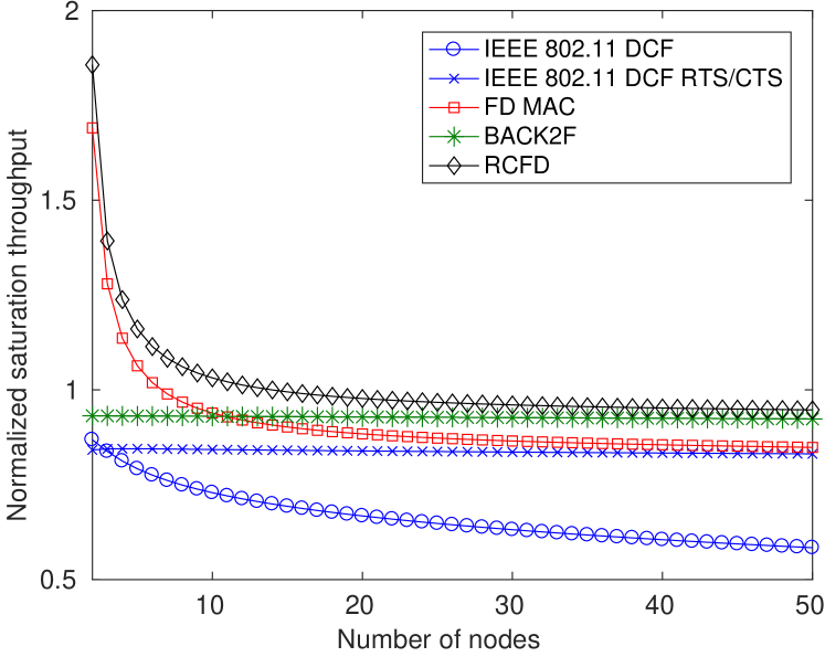
Figure 6: Theoretical saturation throughput versus number of nodes, with L=1000 Bytes long packets and R=6 Mbps data rate.

In the previous subsection we have derived the saturation throughput for the different MAC protocols as a function of several system parameters. We will now numerically evaluate this metric for different network configurations and system parameters. Tab. II reports the simulation parameters in this evaluation, which are adopted from the IEEE 802.11g standard [24].

Fig. 6 shows the saturation throughput for all MAC algorithms versus the number of nodes in the network. The payload length has been kept fixed at $L=1000$ Bytes, while the transmission rate is $R=6$ Mbps, yielding a data transmission time of roughly $T_{d}=1.4$ ms. It can be observed that the RCFD strategy outperforms all other MAC algorithms for any number of nodes. The two schemes that consider FD transmissions (RCFD and FD MAC) are able to provide a normalized throughput higher than one, for a small number of nodes. BACK2F and IEEE 802.11 RTS/CTS do not show a significant variation with the number of nodes, with the first one providing a higher throughput (close to 1) and performing close to RCFD for a large number of nodes. The standard IEEE 802.11 DCF provides the worst performance, strongly affected by the number of nodes, as expected.

It is worth noting that the sharp decrease in throughput presented by FD–capable MAC protocols (RCFD and FD MAC) is due to the FIFO assumption. Indeed, in both cases, assuming that a node $n_{i}$ gets the channel, a FD transmission happens only if the packet at the head of the queue of the receiver $n_{j}$ is destined to $n_{i}$, which happens with probability $1/(N-1)$. The throughput curves for these algorithm, hence, follow a hyperbolic shape. The FIFO assumption was considered in this analysis for the sake of tractability and will be relaxed in the simulations of Section 5.

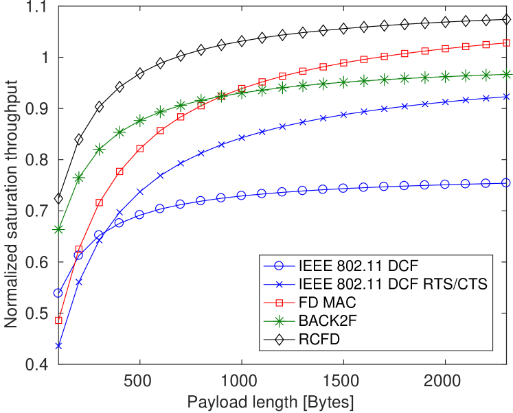
Figure 7: Theoretical saturation throughput versus packet payload size for a network with $N=10$ nodes using an $R=6$ Mbps data rate.

Another evaluation is reported in Fig. 7, where we kept the number of nodes and the data rate fixed at $N=10$ and $R=6$ Mbps, respectively, and we varied the payload length $L$ from 100 to 2300 Bytes. Again, the proposed RCFD technique provides the best performance for all possible payload sizes. The techniques based on time domain RTS/CTS (IEEE 802.11 and FD MAC) perform very poorly for short packets, since in that case the overhead represented by the exchange of RTS and CTS frames has a very significant impact. The techniques that include frequency–based contention (RCFD and BACK2F) are characterized by a similar trend, even if the first one always provides a higher throughput, thanks to its FD capabilities. The standard IEEE 802.11 DCF without RTS/CTS, finally, yields the worst results, since it clearly suffers from the occurrence of collisions.

In order to make an assessment of the numerical results based on the theoretical models presented in this section, a set of network simulations have been performed using the ns3 platform [28], configured according to the following assumptions:

• $N$ nodes are randomly deployed in the same collision domain;

• each node randomly generates packets for every other node in the network and the transmission queue (which follows a FIFO behavior) is always saturated;

• the communication channel is ideal, with collisions being the only source of errors;

• the values of transmission rate ($R=6$ Mbps) and payload size ($L=1000$ Bytes) are fixed.

The results, which refer to the simulation throughput averaged over 10 different simulation runs, are reported in Tab. III, where they are compared with the numerical values of Fig. 6. It can be observed that the results of the analysis and simulations are close. Moreover, the simulations confirm that RCFD outperforms the other channel access schemes for any network size, as the analysis suggested.

TABLE III: Comparison of normalized saturation throughput in analysis and simulations for FD, BACK2F and RCFD channel access schemes

Algorithm	$\mathbf{N=2}$	$\mathbf{N=10}$	$\mathbf{N=20}$	$\mathbf{N=50}$
FD Analysis	1.6908	0.9390	0.8840	0.8485
FD Simulations	1.4281	0.8458	0.7929	0.7377
BACK2F Analysis	0.9319	0.9304	0.9287	0.9235
BACK2F Simulations	0.9312	0.8814	0.8280	0.7016
RCFD Analysis	1.8570	1.0316	0.9773	0.9474
RCFD Simulations	1.8514	0.9306	0.9301	0.9300

5 Simulation assessment

The results of Section 4 show a clear prevalence of the proposed RCFD algorithm over other MAC layer schemes considered. However, the analysis and simulations were conducted under some possibly limiting assumptions, the most important one being that all nodes are within the same collision domain. In order to relax this assumption, the five aforementioned MAC strategies have been compared through ns3, for the case of a wireless network with multiple collision domains.

5.1 Simulations setup

Figure 8: Simulated network for the structured scenario.

The standard distribution of ns3 already contains models for the IEEE 802.11 DCF, both with and without RTS/CTS, as defined in the standard. However, the modules for the MAC algorithms proposed in the literature, namely FD MAC, BACK2F and our proposal RCFD, were not available and therefore had to be purposely developed. Moreover, the standard ns3 wifi module only allows half–duplex communications, preventing a node from transmitting if it is receiving. In order to be able to simulate a network with full–duplex nodes, we adopted the patch discussed in [29], which allows to simulate an FD wireless network with ns3. It is worth stressing that, for the algorithms based on frequency domain operations (BACK2F and RCFD), the exchange of data over OFDM subcarriers during the contention rounds is assumed to be ideal, i.e., when a node transmits on a subcarrier all the other nodes in its collision domain are able to detect it.

Two different scenarios have been simulated: a structured scenario and a random scenario, described in detail in the following.

5.1.1 Setup for the structured scenario

The simulated network for the structured scenario is depicted in Fig. 8. It is an ad hoc wireless network composed of fixed nodes placed on a grid. The distance between two adjacent nodes in the same row or column is $d$. The coverage range of each node is a circle of radius $r=d\sqrt{2}$ and, hence, includes all its one–hop neighbors. Within this area, the node can transmit and receive packets as well as overhear transmissions. To implement this channel model, the RangePropagationLossModel of ns3 has been adopted, combined with a purposely implemented error model. According to these models, a transmission between two nodes is successful only if the distance is below $r$ and there is no collision, and it fails with probability 1 otherwise (regardless of the adopted transmission rate). In this way, the impact of collisions on the network can be accurately analyzed for the different channel access strategies, isolating it from all the other factors that can affect the performance, such as path loss, fading, performance of different modulation and coding schemes, etc.

The total number of nodes in the network is $N=g^{2}$, where $g$ is the grid size, and simulations have been conducted for several values of $g$.

5.1.2 Setup for the random scenario

In the random scenario, $N$ nodes are randomly deployed within a square of size $l$. The coverage range $r$ of a node is determined as the maximum range which allows a success transmission probability above 90% for a packet of size $L$ transmitted with rate $R$ and assuming no fading.

The channel model used in this scenario combines the LogDistancePropagationLossModel for path loss and the NakagamiPropagationLossModel to emulate Rayleigh fading. The NistErrorRateModel validated in [30] was adopted, that takes into account the different robustness levels of each modulation and coding scheme.

The goal of the random scenario is to investigate how the RCFD algorithm proposed in this paper would perform in a more realistic ad hoc wireless network in comparison to the other channel access techniques.

5.1.3 Traffic model and metrics for both scenarios

In each node, several applications are installed, one for each node within its coverage range, as shown in Fig. 8 for the structured scenario. The starting time of each application, $t_{s}$, is distributed as an exponential random variable of parameter $\lambda_{s}$ truncated after $t_{s,max}$, while the stop time coincides with the end of the simulation.

An OnOffApplication model is adopted where the duration of the ON and OFF periods are also exponentially distributed, with mean $T_{ON}$ and $T_{OFF}$, respectively. During the ON period, the applications generates constant bitrate (CBR) traffic with source rate $R_{s}$. All packets have the same length $L$ and the data rate at the physical layer, $R$, is constant.

Network operations have been simulated for a total of $T$ seconds (with the initial transient period removed), for different values of the network size $N$. Given a certain parameter configuration, each simulation has been repeated a total of $N_{S}$ times and results have been averaged.

We considered two performance metrics, namely the normalized system throughput, $\Gamma$, and the average delay, $\Delta$. The normalized system throughput is the ratio of the total number of payload bits successfully delivered by all the nodes in the network over the simulation time $T$, and the offered traffic $G$. The offered traffic is given by

$$G=R_{s}\cdot N_{a}\cdot\frac{T_{ON}}{T_{ON}+T_{OFF}}$$ (27)

where $N_{a}$ is the total number of running applications in the network, which is a function of the network size $N$ and the coverage radius $r$.

The average delay, on the other hand, is the arithmetic mean of the delay experienced by each packet in the network, defined as the time elapsed from the instant in which the packet is generated by the application to the instant in which the packet is successfully delivered or discarded.

Tab. IV reports all the parameters adopted in the simulations.

TABLE IV: Simulation parameters

Parameter	Description	Value
$d$	Distance between two adjacent nodes in the structured scenario	100 m
$l$	Side of deployment area in the random scenario	500 m
$\lambda_{s}$	Parameter of application starting time	$0.5~{}\textrm{s}^{-1}$
$t_{s,max}$	Maximum application starting time	5 s
$T_{ON}$	Average time during which each application is ON	0.1 s
$T_{OFF}$	Average time during which each application is OFF	0.1 s
$R_{s}$	Application source rate during the ON period	1 Mbit/s
$T$	Duration of each simulation	20 s
$N_{tx,max}$	Maximum number of retransmissions at the MAC layer	7
$Q_{max}$	Transmission queue size (packets)	1000
$\Delta_{max}$	Maximum interval after which a packet is discarded	1 s
$L$	Payload length for packets	$\{200,500,1000\}$ Bytes
$R$	Data rate at the PHY layer	$\{6,18,54\}$ Mbit/s
$N_{S}$	Number of simulations for each configuration	10

It is worth noting that the simulation–based results presented in this section are complementary with respect to those presented in Section 4, since the latter were based on the assumption of a single collision domain, whereas in this section we allow multiple collision domains.

5.2 Simulation results for the structured scenario

In order to provide a comprehensive assessment of the presented protocol, in the network simulations we have evaluated its performance in the structured scenario for two opposite cases:

1. Long packet transmission time: in this case large payload packets ($L=1000$ Bytes) were exchanged at the lowest possible rate provided by IEEE 802.11g, namely $R=6$ Mbit/s, resulting in a very long packet transmission time.

2. Short packet transmission time: in this case small payload packets ($L=200$ Bytes) were exchanged at the highest possible rate, namely $R=54$ Mbit/s, with a corresponding short packet transmission time.

In each case, the aforementioned performance metrics for the considered MAC algorithms have been evaluated for different values of the grid size parameter $g$, ranging from 3 ($N=9$ nodes) to 10 ($N=100$ nodes).

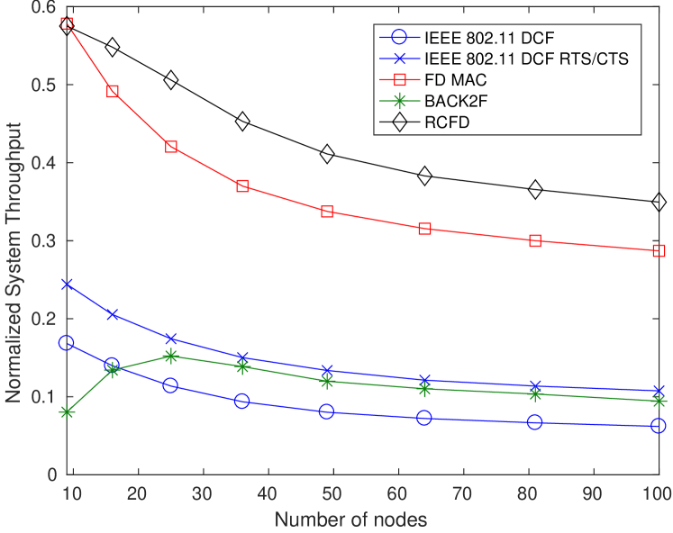
Figure 9: Simulated normalized system throughput $\Gamma$ for the structured scenario, case I ($R=6$ Mbit/s, $L=1000$ Bytes).

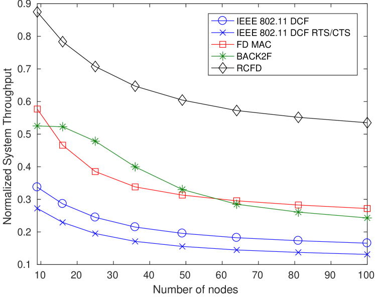
Figure 10: Simulated normalized system throughput $\Gamma$ for the structured scenario, case II ($R=54$ Mbit/s, $L=200$ Bytes).

Fig. 9 shows the normalized system throughput $\Gamma$ for case I. The RCFD strategy outperforms the other MAC protocols for any network size. The FD MAC algorithm is able to achieve similar performance when the number of nodes is small, but its throughput significantly degrades as the network size increases. The BACK2F protocol presents a significantly lower $\Gamma$, due to its difficulties in handling multiple collision domains. Finally, the IEEE 802.11 strategies based on time domain channel contention perform poorly.

The same metric $\Gamma$ is reported in Fig. 10 for the second case. Again, RCFD performs much better than all other strategies. It can be observed, in particular, that the schemes relying upon the exchange of RTS/CTS frames (FD MAC and IEEE 802.11) perform much worse than in the previous case, since these frames represent a significant overhead, given the lower time needed for the actual transmission of data frames. BACK2F, which instead relies on frequency domain contention as RCFD, performs much better than in the previous case, reaching similar performance as FD MAC, despite not being a full–duplex MAC protocol.

It is worth noticing that the normalized throughput values are higher in Fig. 10 with respect to Fig. 9. Indeed, the higher PHY rate allows to exchange an increased amount of data in the same time.

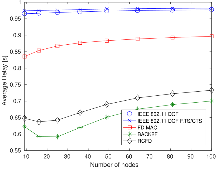
Figure 11: Simulated average delay $\Delta$ for the structured scenario, case II ($R=54$ Mbit/s, $L=200$ Bytes).

The average delay $\Delta$ simulated in case II for all the MAC protocols is shown in Fig. 11. The strategies that include frequency domain channel contention strongly outperform those based on a time domain approach. In particular, BACK2F slightly outperforms the RCFD strategy, mostly due to the lower number of contention rounds in the frequency domain (2 against 3). Similar results are achieved for case I, not reported here for space constraints.

5.3 Simulation results for the random scenario

In the random scenario, the performance of the considered MAC algorithms have been evaluated for different network size values, ranging from $N=10$ to $N=50$ nodes. The payload size has been fixed to $L=500$ Bytes and the PHY layer transmission rate to $R=18$ Mbps, providing an intermediate case between the two extremes analyzed in the structured scenario. Under this configuration, the coverage radius of each node was set to $r=60$ m in order to provide 90% transmission success probability.

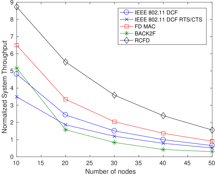
Figure 12: Simulated normalized system throughput $\Gamma$ for the random scenario ($R=18$ Mbit/s, $L=1000$ Bytes).

Fig. 12 shows the normalized system throughput $\Gamma$ for the different MAC algorithms. Also in this case, RCFD is able to significantly outperform all the other schemes. As in case I of the structured scenario, FD MAC provides the closest performance, while the throughput of the BACK2F algorithm suffers from the presence of multiple collision domains and significantly degrades with the network size.

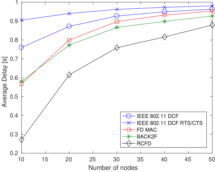
Figure 13: Simulated average delay $\Delta$ for the random scenario ($R=18$ Mbit/s, $L=1000$ Bytes).

The average delay $\Delta$ for the random scenario is reported in Fig. 13. Again, RCFD significantly outperforms all the other schemes, confirming that this strategy represents a very interesting opportunity for real–world applications. Among the other algorithms, BACK2F emerges as the one able to guarantee the lowest delay, thanks to the channel contention in the frequency domain.

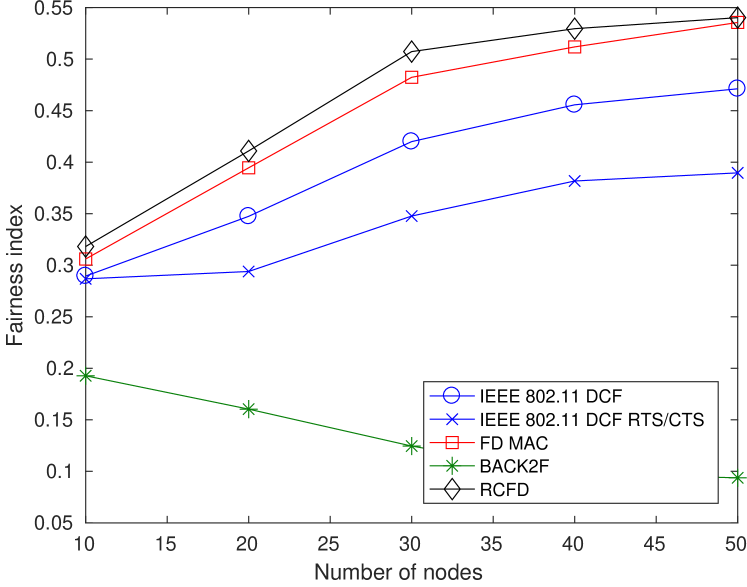
Figure 14: Simulated fairness index $J$ for the random scenario ($R=18$ Mbit/s, $L=1000$ Bytes).

In order to provide a final insight, the fairness of the compared MAC protocols is reported in Fig. 14 for the random scenario, measured in terms of Jain’s fairness index [31], defined as

$$\mathcal{J}\left(p_{1},\dots,p_{N}\right)=\frac{\left(\sum\limits_{i=1}^{N}p_{i}\right)^{2}}{N\cdot\sum\limits_{i=1}^{N}p_{i}^{2}}$$ (28)

where $p_{i}$ is the number of packets successfully received by node $n_{i}$. It can be observed that, also in terms of fairness, RCFD outperforms all other protocols.

6 Conclusions

The currently employed channel access schemes for wireless networks present several issues and relatively low performance. The introduction of full–duplex wireless communication can lead to increased performance but also poses additional challenges to transmission scheduling, and no standard MAC protocol has emerged so far as the best solution for FD wireless networks. In this paper we proposed RCFD, a full–duplex MAC protocol based on a time–frequency channel access procedure. We showed through theoretical analyses and network simulations that this strategy provides excellent performance in terms of both throughput and packet transmission delay, also in the case of dense networks, compared to other standard and state–of–the–art MAC layer schemes.

A natural extension of this work is the experimental assessment of the proposed MAC layer protocol on devices capable of FD operations and able to transmit OFDM symbols using only some specific subcarriers. The optimizations to the presented protocol suggested in Section 3.4 could lead to even higher performance gains with respect to other MAC layer strategies. Also, the protocol can be extended to account for asymmetric full–duplex in addition to bidirectional one. Finally, the performance of RCFD can be tested in the more realistic cases of imperfect FD cancellation and/or mixed networks with both HD and FD nodes.

Appendix A Derivation of transition probabilities for the Markov chain used in the BACK2F analysis

The transition probabilities for the Markov chain defined in Section 4.2 are of the form

$$\footnotesize p_{i,a,j|k,b,l}=P\left\{x(t)=i,c(t)=a,y(t)=j\,|\,x(t-1)=k,c(t-1)=b,y(t-1)=l\right\}$$ (29)

Through some computations, $p_{i,a,j|k,b,l}$ can be factorized in three terms

$$p_{i,a,j|k,b,l}=p_{j|i,a,k,b,l}\cdot p_{i|a,k,b,l}\cdot p_{a|k,b,l}$$ (30)

where

$$p_{j|i,a,k,b,l} =P\{y(t)=j\,|\,x(t)=i,c(t)=a,x(t-1)=k,c(t-1)=b,y(t-1)=l\}$$ (31)

$$p_{i|a,k,b,l} =P\{x(t)=i|c(t)=a,x(t-1)=k,c(t-1)=b,y(t-1)=l\}$$ (32)

$$p_{a|k,b,l} =P\{c(t)=a|x(t-1)=k,c(t-1)=b,y(t-1)=l\}$$ (33)

In the remainder of this appendix, exact expressions for these three terms are derived for all possible values of the parameters $i,a,j,k,b,l$, according to the structure of the BACK2F algorithm, explained in detail in [22] and reported in Algorithm 1 for convenience.

Algorithm 1: BACK2F channel access algorithm [22].

1:procedure BACK2F(packet)

2:    $\mathtt{myback}\leftarrow\mathit{rnd}\left[0,S-1\right]$

3:    wait for $T_{difs}$

4:    if channel is busy then

5:         goto line 2

6:    else

7:         transmit on SC myback in round 1

8:         $\mathtt{minback}\leftarrow$ lowest–frequency SC with signal

9:         $\mathtt{myback}\leftarrow\mathtt{myback}-\mathtt{minback}$

10:         if $\mathtt{myback}>0$ then $\triangleright$ Lost round 1

11:             goto line 2

12:         else

13:             $\mathtt{myback2}\leftarrow\mathit{rnd}\left[0,S-1\right]$

14:             transmit on SC myback2 in round 2

15:             $\mathtt{minback2}\leftarrow$ lowest–frequency SC with signal

16:             if $\mathtt{myback2}=\mathtt{minback2}$ then $\triangleright$ Won round 2

17:                 transmit packet

18:                 goto line 1

19:             else$\triangleright$ Lost round 2

20:                 goto line 2

21:             end if

22:         end if

23:    end if

24:end procedure

A.1 Derivation of $\mathbf{p_{j|i,a,k,b,l}}$

It can first be observed that

$$p_{j|i,a,k,b,l} =P\left\{y(t)=j\,|\,x(t)=i,c(t)=a,x(t-1)=k,c(t-1)=b,y(t-1)=l\right\}$$

$$=P\left\{y(t)=j\,|\,x(t)=i\right\}$$ (34)

since the number of winning nodes at the second round only depends on the number of nodes that have won the first round in the same time slot. We can further state that Eq. (A.1) is meaningful only for $j\leq i$, which leaves only the two following scenarios.

1. $j=i$

   In this case we have $i$ nodes randomly choosing among $S$ subcarriers. The probability that they all pick the same one is given by $1/S^{i-1}$.

2. $j<i$

   The probability that $j$ nodes out of $i$ pick the same SC $c$ and that all the other nodes pick SCs with higher frequency than $c$ is given by

   $${{i}\choose{j}}\left(\frac{1}{S}\right)^{j}\left(1-\frac{c+1}{S}\right)^{i-j}$$ (35)

   This probability has to be summed over all possible SCs except the last one (which would result in all the nodes picking the same one, i.e., $j=i$)

   $$\sum\limits_{c=0}^{S-2}{{i}\choose{j}}\left(\frac{1}{S}\right)^{j}\left(1-\frac{c+1}{S}\right)^{i-j}$$ (36)

Summing up all the scenarios, we obtain the following expression for $p_{j|i,a,k,b,l}$:

$$p_{j|i,a,k,b,l}=\begin{cases}\sum\limits_{c=0}^{S-2}{{i}\choose{j}}\left(\frac{1}{S}\right)^{j}\left(1-\frac{c+1}{S}\right)^{i-j}&\text{if }j<i\\ \frac{1}{S^{i-1}}&\text{if }j=i\\ 0&\text{otherwise}\end{cases}$$ (37)

A.2 Derivation of $\mathbf{p_{i|a,k,b,l}}$

To compute this second term we have to derive the probability that exactly $i$ nodes win the first round at time slot $t$ given that SC $a$ is the lowest–frequency one and that, in the previous time slot, $k$ nodes won the first round (with SC $b$) and $l$ nodes won the second round. Again, we split the problem in multiple scenarios.

1. $k\neq l$

   In this scenario, at the end of time slot $t-1$ we have the following groups of nodes:

   1. $N-k$ nodes that have lost round 1 and, hence, have $\mathtt{myback}>0$ (line 10 in Algorithm 1).

   2. $k-l\neq 0$ nodes that have lost round 2 and, hence, have $\mathtt{myback}=0$ (line 12 in Algorithm 1).

   3. $l$ nodes that have won round 2 and, after transmitting, have $\mathtt{myback}$ randomly distributed between 0 and S-1 (lines 18 and 2 in Algorithm 1).

   Therefore, the following observations can be made:

   • The lowest–frequency SC at time $t$ is 0 (chosen by at least the nodes of group B), hence $p_{i|a,k,b,l}$ is always 0 when $a\neq 0$.

   • There are at least $k-l$ nodes (group B) that have $\mathtt{myback}=0$ and win round 1, hence, $i\geq k-l$.

   • The maximum number of first round winners is $k$, since $N-k$ nodes (group A) have $\mathtt{myback}>0$, hence, $i<k$.

     The probability that $m$ of the $l$ nodes of group C pick 0 as a SC and hence win round 1 at time slot $t$ is

     $${{l}\choose{m}}\left(\frac{1}{S}\right)^{m}\left(1-\frac{1}{S}\right)^{l-m}$$ (38)

     and the corresponding number $i$ of first–round winners is $i=k-l+m$, hence, we obtain $p_{i|a,k,b,l}$ for the case of $a=0$ and $k\neq l$ by replacing $m$ in Eq. (38) with $i-k+l$.

   $$p_{i|a,k,b,l}=\begin{cases}{{l}\choose{i-k+l}}\left(\frac{1}{S}\right)^{i-k+l}\left(1-\frac{1}{S}\right)^{k-i}&\text{if }k\neq l,a=0,k-l\leq i\leq k\\ \frac{{{k}\choose{i}}\left(\frac{1}{S}\right)^{i}\left(1-\frac{1}{S}\right)^{k-i}}{1-\left(1-\frac{1}{S}\right)^{k}}&\text{if }k=l\neq N,a=0,i\leq k\\ {{k}\choose{i-N+k}}\left(\frac{1}{b+1}\right)^{i-N+k}\left(1-\frac{1}{b+1}\right)^{N-i}&\text{if }k\!=\!l\!\neq\!N,a=\!S\!-\!b-\!1,i\!\geq\!N\!-\!k\\ \frac{\left[{{N-k}\choose{n}}\left(\frac{1}{S-b-a}\right)^{n}\left(1-\frac{1}{S-b-a}\right)^{N-k-n}\right]\cdot\left[{{k}\choose{i-n}}\left(\frac{1}{S-a}\right)^{i-n}\left(1-\frac{1}{S-a}\right)^{k-i+n}\right]}{1-\left(1-\frac{1}{S-a}\right)^{k}\left(1-\frac{1}{S-b-a}\right)^{N-k}}&\text{if }k=l\neq N,0<a<S-b-1\\ \frac{{{N}\choose{i}}\left(\frac{1}{S-a}\right)^{i}\left(1-\frac{1}{S-a}\right)^{N-i}}{1-\left(1-\frac{1}{S-a}\right)^{N}}&\text{if }k=l=N\\ 0&\text{otherwise}\end{cases}$$ (44)

2. $k=l\neq N$

   In this scenario, at the end of time slot $t-1$ we have the following group of nodes:

   1. $N-k$ nodes have lost round 1 and, hence, will have $\mathtt{myback}>0$. The maximum value of myback for this node is $S-b-1$, according to line 9 in Algorithm 1 and taking into account that $\mathtt{minback}=b$ (lowest–frequency SC at round 1 in time slot $t-1$).

   2. $k$ nodes have won round 2 and, after transmitting, will have $\mathtt{myback}$ randomly varying between 0 and S-1 (lines 18 and 2 in Algorithm 1).

   The case $a=0$ is trivial, since the maximum number of first round winners is $k$ (analogously to scenario I) and the probability that $i$ nodes out of $k$ (group B) select $\mathtt{myback}=0$ (given that there is at least one node that selects it) is

   $$\frac{{{k}\choose{i}}\left(\frac{1}{S}\right)^{i}\left(1-\frac{1}{S}\right)^{k-i}}{1-\left(1-\frac{1}{S}\right)^{k}}$$ (39)

   Another trivial case is $a=S-b-1$: in this situation, the $N-k$ nodes of group A all win the first round at $t$ (hence $i\geq N-k$) and the probability that $m$ nodes out of the remaining $k$ (group B) select SC $S-b-1$ is

   $${{k}\choose{m}}\left(\frac{1}{b+1}\right)^{m}\left(1-\frac{1}{b+1}\right)^{k-m}$$ (40)

   with $i=N-k+m$.

   The case of $0<a<S-b-1$, instead, is non–trivial, since the nodes from both groups can select $a$ as a SC. In detail, the probability that $n$ nodes from group A and $i-n$ nodes from group B select SC $a$ (given that at least one node selects it) is given by

   $$\frac{\left[{{N-k}\choose{n}}\left(\frac{1}{S-b-a}\right)^{n}\left(1-\frac{1}{S-b-a}\right)^{N-k-n}\right]\cdot\left[{{k}\choose{i-n}}\left(\frac{1}{S-a}\right)^{i-n}\left(1-\frac{1}{S-a}\right)^{k-i+n}\right]}{1-\left(1-\frac{1}{S-a}\right)^{k}\left(1-\frac{1}{S-b-a}\right)^{N-k}}$$ (41)

   The expression in Eq. (41) has to be summed for all possible values of $n$, taking into account that $0\leq n\leq i$ by definition, and also $n\leq N-k$ and $i-n\leq k$. Therefore, the probability that $i$ nodes win the first round at time $t$ when $k=l\neq N$ and $0<a<S-b-1$ is

   $$\footnotesize\frac{\sum\limits_{n=\max(i-k,0)}^{min(N-k,i)}\left[{{N-k}\choose{n}}\left(\frac{1}{S-b-a}\right)^{n}\left(1-\frac{1}{S-b-a}\right)^{N-k-n}\right]\cdot\left[{{k}\choose{i-n}}\left(\frac{1}{S-a}\right)^{i-n}\left(1-\frac{1}{S-a}\right)^{k-i+n}\right]}{1-\left(1-\frac{1}{S-a}\right)^{k}\left(1-\frac{1}{S-b-a}\right)^{N-k}}$$ (42)

3. $k=l=N$

   In this scenario there is only one group of $N$ nodes, which have all won the second round in time slot $t-1$ and hence can select myback in the range $[a,S-1]$. The probability that exactly $i$ nodes select $\mathtt{myback}=a$ (given that at least one selects it) is given by

   $$\frac{{{N}\choose{i}}\left(\frac{1}{S-a}\right)^{i}\left(1-\frac{1}{S-a}\right)^{N-i}}{1-\left(1-\frac{1}{S-a}\right)^{N}}$$ (43)

Summing up all the scenarios, we obtain the expression for $p_{i|a,k,b,l}$ reported in Eq. (44).

A.3 Derivation of $\mathbf{p_{a|k,b,l}}$

To compute the third and last term, we have to derive the probability that SC $a$ is the lowest–frequency one at the first contention round during time slot $t$, given that, in the previous time slot, $k$ nodes won the first round (with SC $b$) and $l$ nodes won the second round. We consider the same three scenarios as in Sec. A.2, thus, for each scenario, we refer to the same groups of nodes.

1. $k\neq l$

   As explained in Sec. A.2, the only possible value for $a$ in this scenario is 0, hence $p_{0|k,b,l}=1$ and 0 otherwise.

2. $k=l\neq N$

   As explained in Sec. A.2, the case $a=0$ is trivial, since it can only happen for the $k$ nodes of group B and it happens with probability

   $$1-\left(1-\frac{1}{S}\right)^{k}$$ (44)

   $$p_{a|k,b,l}=\begin{cases}1&\text{if }k\neq l,a=0\\ 1-\left(1-\frac{1}{S}\right)^{k}&\text{if }k=l\neq N,a=0\\ \left(1-\frac{a}{S}\right)^{k}\left(1-\frac{a-1}{S-b-1}\right)^{N-k}-\left(1-\frac{a+1}{S}\right)^{k}\left(1-\frac{a}{S-b-1}\right)^{N-k}&\text{if }k\!=\!l\!\neq\!N,0\!<\!a\!\leq\!S\!-\!b\!-\!1\\ \left(1-\frac{a}{S}\right)^{N}-\left(1-\frac{a+1}{S}\right)^{N}&\text{if }k=l=N\\ 0&\text{otherwise}\end{cases}$$ (52)

   
   

   The case $a>0$, instead, is non–trivial. We also have that $a\leq S-b-1$, as discussed in Sec. A.2. Let us indicate with a random variable $X_{i},i=1,\dots,S-b-1$ the number of nodes in group A that select SC $i$ at the first round and with $Y_{j},j=0,\dots,S-1$ the number of nodes in group B that select SC $j$ at the first round. Both these groups of random variables follow a multinomial distribution with constant probabilities $p_{i}=\frac{1}{S-b-1}$ for the first group and $p_{j}=\frac{1}{S}$ for the second group. The probability that $a$ is the lowest–frequency SC is expressed as

   $$p_{a|k,b,l}=p_{X,a}\cdot p_{Y,a}+p_{X,a}\cdot p_{Y,\bar{a}}+p_{X,\bar{a}}\cdot p_{Y,a}$$ (45)

   where:

   $$p_{X,a} =P\left\{X_{1}=0,\dots,X_{a-1}=0,X_{a}\neq 0\right\}$$

   $$=P\left\{X_{1}=0,\dots,X_{a-1}=0\right\}-P\left\{X_{1}=0,\dots,X_{a}=0\right\}$$

   $$=\left(1-\frac{a-1}{S-b-1}\right)^{N-k}-\left(1-\frac{a}{S-b-a}\right)^{N-k}$$ (46)

   $$p_{X,\bar{a}} =P\left\{X_{1}=0,\dots,X_{a}=0\right\}$$

   $$=\left(1-\frac{a}{S-b-a}\right)^{N-k}$$ (47)

   $$p_{Y,a} =P\left\{Y_{0}=0,\dots,Y_{a-1}=0,Y_{a}\neq 0\right\}$$

   $$=P\left\{Y_{0}=0,\dots,Y_{a-1}=0\right\}-P\left\{Y_{1}=0,\dots,Y_{a}=0\right\}$$

   $$=\left(1-\frac{a}{S}\right)^{k}-\left(1-\frac{a+1}{S}\right)^{k}$$ (48)

   $$p_{Y,\bar{a}} =P\left\{Y_{0}=0,\dots,Y_{a}=0\right\}$$

   $$=\left(1-\frac{a+1}{S}\right)^{k}$$ (49)

   The expression for $p_{a|k,b,l}$ when $k=l\neq N$ and $a>0$ can hence be obtained by inserting Eq. (46), (47), (48) and (49) in Eq. (45)

   $$\left(1-\frac{a}{S}\right)^{k}\left(1-\frac{a-1}{S-b-1}\right)^{N-k}-\left(1-\frac{a+1}{S}\right)^{k}\left(1-\frac{a}{S-b-1}\right)^{N-k}$$ (50)

3. $k=l=N$

   In this scenario there is only one group of $N$ nodes, which have all won the second round at time slot $t-1$ and hence can select myback in the range $[0,S-1]$. Let us indicate with a random variable $Z_{i},i=0,\dots,S-1$ the number of nodes that select SC $i$ at the first round, multinomially distributed with constant probability $p_{i}=\frac{1}{S}$. The probability that $a$ is the lowest–frequency SC is expressed as

   $$p_{a|k,b,l} =P\left\{Z_{0}=0,\dots,Z_{a-1}=0,Z_{a}\neq 0\right\}$$

   $$=P\left\{Z_{0}=0,\dots,Z_{a-1}=0\right\}-P\left\{Z_{0}=0,\dots,Z_{a}=0\right\}$$

   $$=\left(1-\frac{a}{S}\right)^{N}-\left(1-\frac{a+1}{S}\right)^{N}$$ (51)

Summing up all the scenarios, we obtain the expression for $p_{a|k,b,l}$ reported in Eq. (52).

References

- [1] M. Luvisotto, A. Sadeghi, F. Lahouti, S. Vitturi, and M. Zorzi, “RCFD: A Frequency–Based Channel Access Scheme for Full–Duplex Wireless Networks,” in Proceedings of the IEEE International Conference on Communications (ICC), May 2016.
- [2] L. Wang, K. Wu, and M. Hamdi, “Combating Hidden and Exposed Terminal Problems in Wireless Networks,” IEEE Transactions on Wireless Communications, vol. 11, no. 11, pp. 4204–4213, November 2012.
- [3] J. I. Choi, M. Jain, K. Srinivasan, P. Levis, and S. Katti, “Achieving Single Channel, Full Duplex Wireless Communication,” in Proceedings of the 16th ACM Annual International Conference on Mobile Computing and Networking (MobiCom), September 2010.
- [4] M. Duarte and A. Sabharwal, “Full-duplex wireless communications using off-the-shelf radios: Feasibility and first results,” in Proceedings of the 44th Asilomar Conference on Signals, Systems and Computers (ASILOMAR), November 2010.
- [5] S. Chen, M. Beach, and J. McGeehan, “Division-free duplex for wireless applications,” Electronics Letters, vol. 34, no. 2, pp. 147–148, January 1998.
- [6] B. Radunovic, D. Gunawardena, P. Key, A. Proutiere, N. Singh, V. Balan, and G. Dejean, “Rethinking Indoor Wireless Mesh Design: Low Power, Low Frequency, Full-duplex,” in Proceedings of the IEEE International Conference on Sensing, Communication and Networking (SECON), June 2010.
- [7] A. Sabharwal, P. Schniter, D. Guo, D. Bliss, S. Rangarajan, and R. Wichman, “In-Band Full-Duplex Wireless: Challenges and Opportunities,” IEEE Journal on Selected Areas in Communications, vol. 32, no. 9, pp. 1637–1652, September 2014.
- [8] D. Kim, H. Lee, and D. Hong, “A Survey of In-band Full-duplex Transmission: From the Perspective of PHY and MAC Layers,” IEEE Communications Surveys and Tutorials, vol. 17, no. 4, pp. 2017–2046, October 2015.
- [9] M. Jain, J. I. Choi, T. Kim, D. Bharadia, S. Seth, K. Srinivasan, P. Levis, S. Katti, and P. Sinha, “Practical, Real-time, Full Duplex Wireless,” in Proceedings of the 17th ACM Annual International Conference on Mobile Computing and Networking (MobiCom), September 2011, pp. 301–312.
- [10] A. Sahai, G. Patel, and A. Sabharwal, “Pushing the limits of full-duplex: Design and real-time implementation,” Rice University Technical Report TREE1104, 2011.
- [11] J. Y. Kim, O. Mashayekhi, H. Qu, M. Kazandjieva, and P. Levis, “Janus: A novel MAC protocol for full duplex radio,” Stanford University, Computer Science Technical Reports (CSTR), July 2013.
- [12] W. Choi, H. Lim, and A. Sabharwal, “Power-Controlled Medium Access Control Protocol for Full-Duplex WiFi Networks,” IEEE Transactions on Wireless Communications, vol. 14, no. 7, pp. 3601–3613, July 2015.
- [13] N. Singh, D. Gunawardena, A. Proutiere, B. Radunović, H. V. Balan, and P. Key, “Efficient and fair MAC for wireless networks with self-interference cancellation,” in Proceedings of the IEEE International Symposium on Modeling and Optimization of Mobile, Ad Hoc, and Wireless Networks (WiOpt), May 2011, pp. 94–101.
- [14] M. Duarte, A. Sabharwal, V. Aggarwal, R. Jana, K. Ramakrishnan, C. Rice, and N. Shankaranarayanan, “Design and Characterization of a Full-Duplex Multiantenna System for WiFi Networks,” IEEE Transactions on Vehicular Technology, vol. 63, no. 3, pp. 1160–1177, March 2014.
- [15] W. Cheng, X. Zhang, and H. Zhang, “RTS/FCTS mechanism based full-duplex MAC protocol for wireless networks,” in Proceedings of the IEEE Global Communications Conference (GLOBECOM), December 2013, pp. 5017–5022.
- [16] S. Goyal, P. Liu, O. Gurbuz, E. Erkip, and S. Panwar, “A distributed MAC protocol for full duplex radio,” in Proceedings of the 47th Asilomar Conference on Signals, Systems and Computers (ASILOMAR), November 2013, pp. 788–792.
- [17] K. Miura and M. Bandai, “Node architecture and MAC protocol for full duplex wireless and directional antennas,” Proceedings of the IEEE International Symposium on Personal, Indoor and Mobile Radio Communications (PIMRC), pp. 369–374, September 2012.
- [18] A. Sadeghi, S. Mosavat-Jahromi, F. Lahouti, and M. Zorzi, “Multi-hop wireless transmission with half duplex and imperfect full duplex relays,” in Proceedings of the 7th IEEE International Symposium on Telecommunications (IST), September 2014, pp. 1026–1029.
- [19] K. Tamaki, A. Raptino H., Y. Sugiyama, M. Bandai, S. Saruwatari, and T. Watanabe, “Full Duplex Media Access Control for Wireless Multi-Hop Networks,” Proceedings of the 77th IEEE Vehicular Technology Conference (VTC), June 2013.
- [20] W. Zhou, K. Srinivasan, and P. Sinha, “RCTC: Rapid Concurrent Transmission Coordination in Full Duplex Wireless Networks,” in Proceedings of the 21st IEEE International Conference on Network Protocols (ICNP), October 2013.
- [21] S. Sen, R. R. Choudhury, and S. Nelakuditi, “Listen (on the frequency domain) before you talk,” in Proceedings of the 9th ACM SIGCOMM Workshop on Hot Topics in Networks, October 2010.
- [22] S. Sen, R. Roy Choudhury, and S. Nelakuditi, “No time to countdown: migrating backoff to the frequency domain,” in Proceedings of the 17th ACM Annual International Conference on Mobile Computing and Networking (MobiCom), September 2011, pp. 241–252.
- [23] J. Zhang and Q. Zhang, “Use your frequency wisely: Explore frequency domain for channel contention and ACK,” in Proceedings of the IEEE International Conference on Computer Communications (INFOCOM), March 2012, pp. 549–557.
- [24] IEEE Standard for Information technology–Telecommunications and information exchange between systems–Local and metropolitan area networks–Specific requirements. Part 11: Wireless LAN Medium Access Control (MAC) and Physical Layer (PHY) Specifications, IEEE Std., March 2012.
- [25] E. Perahia and R. Stacey, Next Generation Wireless LANs: 802.11n and 802.11ac. Cambridge University Press, 2013.
- [26] D. Bharadia, E. McMilin, and S. Katti, “Full Duplex Radios,” in Proceedings of the ACM Special Interest Group on Data Communication Conference (SIGCOMM), August 2013, pp. 375–386.
- [27] G. Bianchi, “Performance analysis of the IEEE 802.11 distributed coordination function,” IEEE Journal on Selected Areas in Communications, vol. 18, no. 3, pp. 535–547, March 2000.
- [28] The Network Simulator - ns-3. [Online]. Available: http://www.nsnam.org/
- [29] W. Zhou and K. Srinivasan, “SIM+: A simulator for full duplex communications,” in Proceedings of the IEEE International Conference on Signal Processing and Communications (SPCOM), July 2014.
- [30] G. Pei and T. R. Henderson, “Validation of OFDM error rate model in ns-3,” Boeing Research Technology, pp. 1–15, 2010.
- [31] R. Jain, D.-M. Chiu, and W. R. Hawe, A quantitative measure of fairness and discrimination for resource allocation in shared computer system. Eastern Research Laboratory, Digital Equipment Corporation Hudson, MA, 1984, vol. 38.