Enhancing stability of correction procedure via reconstruction using summation-by-parts operators I: Artificial dissipation

Abstract

The correction procedure via reconstruction (CPR, also known as flux reconstruction) is a framework of high order semidiscretisations used for the numerical solution of hyperbolic conservation laws. Using a reformulation of these schemes relying on summation-by-parts (SBP) operators and simultaneous approximation terms (SATs), artificial dissipation / spectral viscosity operators are investigated in this first part of a series. Semidiscrete stability results for linear advection and Burgers’ equation as model problems are extended to fully discrete stability by an explicit Euler method. As second part of this series, Glaubitz, Ranocha, Öffner, and Sonar (Enhancing stability of correction procedure via reconstruction using summation-by-parts operators II: Modal filtering, 2016) investigate connections to modal filters and their application instead of artificial dissipation.

1 Introduction

Many fundamental physical principles can be described by balance laws. Without additional source terms, they reduce to (hyperbolic systems of) conservation laws. These types of partial differential equations can be used inter alia as models in fluid dynamics, electrodynamics, space and plasma physics.

Traditionally, low order numerical methods have been used to solve hyperbolic conservation laws, especially in industrial applications. These methods can have excellent stability properties but also excessive numerical dissipation. Thus, they become very costly for high accuracy or long time simulations. Therefore, in order to use modern computing power more efficiently, high order methods provide a viable alternative. However, these methods often lack desired stability properties.

The flux reconstruction (FR) method has been established by [8] as a framework of high order semidiscretisations recovering some well known schemes such as spectral difference (SV) and discontinuous Galerkin (DG) methods with special choices of the parameters. Later, [9] reviewed these schemes and coined the common name correction procedure via reconstruction (CPR).

Linearly stable schemes have been proposed by [23, 24], extending an idea of [10]. However, nonlinear stability is much more difficult and has been considered inter alia by [11, 26].

[20, 19, 18] provided a reformulation of CPR methods in the general framework of summation-by-parts (SBP) operators using simultaneous approximation terms (SATs). These techniques originate in finite difference (FD) methods and have been used as building blocks of provably stable discretisations, especially for linear (or linearised) problems. Reviews of these schemes as well as historical and recent developments have been published by [21, 17, 3]. Generalised SBP operators have been introduced inter alia by [4, 2] and extensions to multiple dimensions not relying on a tensor product structure by [7, 18].

However, SBP operators with SATs have been used predominantly to create provably stable semidiscretisations, although they can also be applied for implicit time integration algorithms. Contrary, using a simple explicit Euler method as time discretisation, semidiscrete stability is not sufficient for a stable fully discrete scheme, as described inter alia in section 3.9 of [20].

Artificial dissipation / spectral viscosity has already been used in the early works of [25] to enhance stability of numerical schemes for conservation laws. [15] used artificial dissipation in the FD framework of SBP operators and SATs. Further developments and results about artificial dissipation / spectral viscosity have been published inter alia by [22, 13, 14, 16].

In this work, the application of artificial dissipation / spectral viscosity in the context of CPR methods using SBP operators is investigated. Therefore, the framework of [20, 19, 18] is presented in section 2. Since SBP operators mimic integration by parts on a discrete level, artificial dissipation operators are introduced at first in the continuous setting in section 3. Using a special representation of these viscosity operators in the semidiscrete setting, conservation and stability are desired properties reproduced analogously. Additionally, the discrete eigenvalues are compared with their continuous counterparts obtained for Legendre polynomials. Fully discrete schemes are obtained by an explicit Euler method and a new algorithm to adapt the strength of the artificial dissipation is proposed, yielding stable fully discrete schemes if the time step is small enough. The theoretical results are augmented by numerical experiments in section 4. Finally, a conclusion is presented in section 5, together with additional topics of further research, inter alia the connections to modal filters described in the second part of this series [5].

2 Correction procedure via reconstruction using summation-by-parts operators

In this section, the formulation of CPR methods using SBP operators given by [20] will be described. Additionally, $L_{2}$ stable semidiscretisation will be presented for two model problems in one spatial dimension: linear advection with constant velocity and Burgers’ equation.

2.1 Correction procedure via reconstruction

The correction procedure via reconstruction is a semidiscretisation using a polynomial approximation on elements. In order to describe the basic idea, a scalar conservation law in one space dimension

$$\partial_{t}u+\partial_{x}f(u)=0,$$ (1)

equipped with appropriate initial and boundary conditions will be used. Since the focus does not lie on the implementation of boundary conditions, a compactly supported initial condition or periodic boundary conditions will be assumed.

The domain $\Omega\subset\mathbb{R}$ is divided into disjoint open intervals $\Omega_{i}\subset\Omega$ such that $\bigcup_{i}\overline{\Omega}_{i}=\Omega$. These elements $\Omega_{i}$ are mapped diffeomorphically onto a standard element, which is simply the interval $(-1,1)$ and can be realised by an affine linear transformation in this case. In the following, all computations are performed in this standard element.

On each element $\Omega_{i}$, the solution $u(t)=u(t,\cdot)$ is approximated by a polynomial of degree $\leq p\in\mathbb{N}_{0}$. Classically, a nodal Lagrange basis is used. Thus, the coefficients of $\underline{u}$ are nodal values $\underline{u}_{i}=u(\xi_{i}),i\in\mathinner{\left\{0,\dots,p\right\}}$, where $-1\leq\xi_{i}\leq 1$ are distinct points in $[-1,1]$.

Since CPR methods are polynomial collocation schemes, the flux $f(u)$ is approximated by the polynomial $\underline{f}$ interpolating at the nodes $\xi_{i}$, i.e. $\underline{f}_{i}=f\left(\underline{u}_{i}\right)=f\left(u(\xi_{i})\right)$. Using a discrete derivative matrix $\underline{\underline{D}}\,$, the divergence of $\underline{f}$ is $\underline{\underline{D}}\,\underline{f}$. However, since the solutions will probably be discontinuous across elements, the discrete flux will have jump discontinuities, too.

Additionally, in order to include the effects of neighbouring elements, a correction of the discontinuous flux is performed. Therefore, the solution polynomial $\underline{u}$ is interpolated to the left and right boundary yielding the values $u_{L},u_{R}$. Thus, at each boundary node, there are two values $u_{-},u_{+}$ of the elements on the left and right hand side, respectively. A continuous corrected flux with the common value of a numerical flux $f^{\mathrm{num}}(u_{-},u_{+})$ (Riemann solver) at the boundary shall be used. Therefore, the flux $\underline{f}$ is interpolated to the boundaries yielding $f_{L},f_{R}$, and left and right correction functions $g_{L},g_{R}$ are introduced. These functions are symmetric, i.e. $g_{L}(x)=g_{R}(-x)$, approximate zero in $(-1,1)$ and fulfil $g_{L}(-1)=g_{R}(1)=1,g_{L}(1)=g_{R}(-1)=0$. Finally, the time derivative is computed via

$$\partial_{t}\underline{u}=-\underline{\underline{D}}\,\underline{f}-(f^{\mathrm{num}}_{L}-f_{L})\underline{g^{\prime}}_{L}-(f^{\mathrm{num}}_{R}-f_{R})\underline{g^{\prime}}_{R}.$$ (2)

Using a restriction matrix $\underline{\underline{R}}\,$ performing interpolation to the boundary, a correction matrix $\underline{\underline{C}}\,=\left(\underline{g^{\prime}}_{L},\underline{g^{\prime}}_{R}\right)$, and writing $\underline{f}^{\mathrm{num}}=(f^{\mathrm{num}}_{L},f^{\mathrm{num}}_{R})^{T}$, [20] reformulated this as

$$\partial_{t}\underline{u}=-\underline{\underline{D}}\,\underline{f}-\underline{\underline{C}}\,\left(\underline{f}^{\mathrm{num}}-\underline{\underline{R}}\,\underline{f}\right).$$ (3)

Using a nodal basis associated with a quadrature rule using weights $\omega_{0},\dots,\omega_{p}$, the mass matrix $\underline{\underline{M}}\,=\operatorname{diag}(\omega_{0},\dots,\omega_{p})$ is diagonal and corresponds to an SBP operator, i.e. using the boundary matrix $\underline{\underline{B}}\,=\operatorname{diag}(-1,1)$, integration by parts

$$\int_{\Omega}u\,\partial_{x}v+\int_{\Omega}\partial_{x}u\,v=u\,v\big{|}_{\partial\Omega}$$ (4)

is mimicked on a discrete level by summation-by-parts

$$\underline{u}^{T}\underline{\underline{M}}\,\underline{\underline{D}}\,\underline{v}+\underline{u}^{T}\underline{\underline{D}}{{}^{T}}\underline{\underline{M}}\,\underline{v}=\underline{u}^{T}\underline{\underline{R}}{{}^{T}}\underline{\underline{B}}\,\underline{\underline{R}}\,\underline{v},$$ (5)

since the SBP property

$$\underline{\underline{M}}\,\underline{\underline{D}}\,+\underline{\underline{D}}{{}^{T}}\underline{\underline{M}}\,=\underline{\underline{R}}{{}^{T}}\underline{\underline{B}}\,\underline{\underline{R}}\,$$ (6)

is fulfilled. Here, either a Gauß-Legendre basis without boundary nodes or a Lobatto-Legendre basis including both boundary nodes is used. The associated quadrature rules are exact for polynomials of degree $\leq 2p+1$ and $\leq 2p-1$, respectively.

This concept has been generalised by [19] to finite dimensional Hilbert spaces $X_{V},X_{B}$ of functions on the volume $\Omega$ and boundary $\partial\Omega$, respectively. Choosing appropriate bases $\mathcal{B}_{V}$ and $\mathcal{B}_{B}$, the scalar product on the volume approximates the $L_{2}$ scalar product

$$\left\langle{u,v}\right\rangle_{M}=\underline{u}^{T}\underline{\underline{M}}\,\underline{v}\approx\int_{\Omega}u\,v=\left\langle{u,v}\right\rangle_{L_{2}}$$ (7)

and is represented by $\underline{\underline{M}}\,$. The divergence operator is $\underline{\underline{D}}\,$, the scalar product on the boundary with prepended multiplication with the outer normal is represented by $\underline{\underline{B}}\,$, and the restriction to the boundary by $\underline{\underline{R}}\,$. In this way, also modal Legendre bases are allowed and fulfil the SBP property (6).

The correction term $\underline{\underline{C}}\,\left(\underline{f}^{\mathrm{num}}-\underline{\underline{R}}\,\underline{f}\right)$ of the semidiscretisation (3) corresponds to a simultaneous approximation term in the framework of SBP methods. In general, the canonical choice of correction matrix presented by [20] is

$$\underline{\underline{C}}\,=\underline{\underline{M}}{{}^{-1}}\underline{\underline{R}}{{}^{T}}\underline{\underline{B}}\,.$$ (8)

However, using different choices yields the full range of energy stable schemes derived by [23, 24].

2.2 Linear advection

The linear advection equation with constant velocity is a scalar conservation law with linear flux $f(u)=u$, i.e.

$$\partial_{t}u+\partial_{x}u=0.$$ (9)

The canonical choice (8) of the correction matrix yields the semidiscretisation

$$\partial_{t}\underline{u}=-\underline{\underline{D}}\,\underline{u}-\underline{\underline{M}}{{}^{-1}}\underline{\underline{R}}{{}^{T}}\underline{\underline{B}}\,\left(\underline{f}^{\mathrm{num}}-\underline{\underline{R}}\,\underline{u}\right)$$ (10)

in the standard element, which is conservative across elements and stable with respect to the discrete norm $\mathinner{\!\left\lVert\cdot\right\rVert}_{M}$ induced by $\underline{\underline{M}}\,$, if an adequate numerical flux is chosen, see inter alia Theorem 5 of [20].

2.3 Burgers’ equation

Burgers’ equation

$$\partial_{t}u+\partial_{x}\frac{u^{2}}{2}=0$$ (11)

is nonlinear. Since the product of two polynomials of degree $\leq p$ is in general a polynomial of degree $\leq 2p$, it has to be projected onto the lower dimensional space of polynomials of degree $\leq p$. For a nodal (Gauß-Legendre or Lobatto-Legendre) basis, the collocation approach is used, i.e. the linear operator representing multiplication with $\underline{u}$ is given by a diagonal matrix

$$\underline{\underline{u}}\,=\operatorname{diag}(\underline{u})=\operatorname{diag}(\underline{u}_{0},\dots,\underline{u}_{p})=\operatorname{diag}(u(\xi_{0}),\dots,u(\xi_{p})).$$ (12)

For a modal Legendre basis, an exact multiplication of polynomials followed by an exact $L_{2}$ projection is used for the multiplication.

Using the $\underline{\underline{M}}\,$-adjoint $\underline{\underline{u}}{{}^{*}}=\underline{\underline{M}}{{}^{-1}}\underline{\underline{u}}{{}^{T}}\underline{\underline{M}}\,$, [19] presented the semidiscretisation

$$\partial_{t}\underline{u}=-\frac{1}{3}\underline{\underline{D}}\,\underline{\underline{u}}\,\underline{u}-\frac{1}{3}\underline{\underline{u}}\,{{}^{*}}\underline{\underline{D}}\,\underline{u}+\underline{\underline{M}}{{}^{-1}}\underline{\underline{R}}{{}^{T}}\underline{\underline{B}}\,\left(\underline{f}^{\mathrm{num}}-\frac{1}{3}\underline{\underline{R}}\,\underline{\underline{u}}\,\underline{u}-\frac{1}{6}\left(\underline{\underline{R}}\,\underline{u}\right)^{2}\right),$$ (13)

which is conservative across elements and stable in the discrete norm induced by $\underline{\underline{M}}\,$, if an appropriate numerical flux is chosen, see inter alia Theorem 2 of [19].

3 Artificial dissipation / spectral viscosity

As in the previous section, a scalar conservation law in one space dimension

$$\partial_{t}u(t,x)+\partial_{x}f\left(u(t,x)\right)=0$$ (14)

with adequate initial and periodic boundary conditions is considered. The introduction of a viscosity term on the right-hand side yields

$$\partial_{t}u(t,x)+\partial_{x}f\left(u(t,x)\right)=(-1)^{s+1}\varepsilon\left(\partial_{x}a(x)\partial_{x}\right)^{s}u(t,x),$$ (15)

where $s\in\mathbb{N}$ is the order, $\varepsilon\geq 0$ the strength and $a\colon\mathbb{R}\to\mathbb{R}$ is a suitable function. The term $\left(\partial_{x}a(x)\partial_{x}\right)^{s}$ describes the $s$-fold application of the linear operator $f(x)\mapsto\partial_{x}\left(a(x)\partial_{x}f(x)\right)$. In the following, the dependence on $t$ and $x$ will be implied but not written explicitly in all cases.

3.1 Continuous setting

In order to investigate conservation (assuming a suitably regular solution $u$), equation (15) is integrated over some interval $\Omega$, resulting in

$$\dfrac{\operatorname{d\!}{}}{\operatorname{d\!}{t}}\int_{\Omega}u=\int_{\Omega}\partial_{t}u=-\int_{\Omega}\partial_{x}f(u)+(-1)^{s+1}\varepsilon\int_{\Omega}\left(\partial_{x}a\partial_{x}\right)^{s}u.$$ (16)

Carrying out the integration on the right hand side yields

$$\dfrac{\operatorname{d\!}{}}{\operatorname{d\!}{t}}\int_{\Omega}u =-f(u)\big{|}_{\partial\Omega}+(-1)^{s+1}\varepsilon\,a\,\partial_{x}\left(\partial_{x}a\partial_{x}\right)^{s-1}u\big{|}_{\partial\Omega}.$$ (17)

Thus, if $a$ vanishes at the boundary $\partial\Omega$ of the interval $\Omega$, the rate of change of $\int_{\Omega}u$ is given by the flux of $f(u)$ through the surface $\partial\Omega$, just as for the scalar conservation law (1) with vanishing right hand side.

Investigating $L_{2}$ stability, equation (15) is multiplied with the solution $u$ and integrated over $\Omega$

$$\frac{1}{2}\dfrac{\operatorname{d\!}{}}{\operatorname{d\!}{t}}\mathinner{\!\left\lVert u\right\rVert}_{L_{2}(\Omega)}^{2}=\frac{1}{2}\dfrac{\operatorname{d\!}{}}{\operatorname{d\!}{t}}\int_{\Omega}u^{2}=\int_{\Omega}u\,\partial_{t}u=-\int_{\Omega}u\,\partial_{x}f(u)+(-1)^{s+1}\varepsilon\int_{\Omega}u\left(\partial_{x}a\partial_{x}\right)^{s}u.$$ (18)

Introducing the entropy flux $F(u)$ by requiring $F^{\prime}(u)=u\,f^{\prime}(u)$, the first term on the right hand side can be rewritten as $-\int_{\Omega}\partial_{x}F(u)$, since $\partial_{x}F(u)=F^{\prime}(u)\partial_{x}u=uf^{\prime}(u)\partial_{x}u=u\partial_{x}f(u)$. Applying integration by parts results in

$$\frac{1}{2}\dfrac{\operatorname{d\!}{}}{\operatorname{d\!}{t}}\mathinner{\!\left\lVert u\right\rVert}_{L_{2}(\Omega)}^{2}= -F(u)\big{|}_{\partial\Omega}+(-1)^{s+1}\varepsilon\,u\,a\,\partial_{x}\left(\partial_{x}a\partial_{x}\right)^{s-1}u\big{|}_{\partial\Omega}$$ (19)

$$+(-1)^{s}\varepsilon\int_{\Omega}\left(a\partial_{x}u\right)\,\partial_{x}\left(\partial_{x}a\partial_{x}\right)^{s-1}u.$$

Assuming again that $a$ vanishes at the boundary $\partial\Omega$, this can be rewritten as

$$\frac{1}{2}\dfrac{\operatorname{d\!}{}}{\operatorname{d\!}{t}}\mathinner{\!\left\lVert u\right\rVert}_{L_{2}(\Omega)}^{2} =-F(u)\big{|}_{\partial\Omega}+(-1)^{s}\varepsilon\int_{\Omega}\left(a\partial_{x}u\right)\,\partial_{x}\left(\partial_{x}a\partial_{x}\right)^{s-1}u$$ (20)

$$=-F(u)\big{|}_{\partial\Omega}+(-1)^{s+1}\varepsilon\int_{\Omega}\left[\left(\partial_{x}a\partial_{x}\right)u\right]\left[\left(\partial_{x}a\partial_{x}\right)^{s-1}u\right].$$

Using induction, this becomes

$$\frac{1}{2}\dfrac{\operatorname{d\!}{}}{\operatorname{d\!}{t}}\mathinner{\!\left\lVert u\right\rVert}_{L_{2}(\Omega)}^{2}=-F(u)\big{|}_{\partial\Omega}+\begin{cases}(-1)^{s+1}\varepsilon\int_{\Omega}\left[\left(\partial_{x}a\partial_{x}\right)^{s/2}u\right]^{2},&s\text{ even},\\ (-1)^{s}\varepsilon\int_{\Omega}a\left[\partial_{x}\left(\partial_{x}a\partial_{x}\right)^{\frac{s-1}{2}}u\right]^{2},&s\text{ odd}.\end{cases}$$ (21)

Thus, if $a$ vanishes at the boundary $\partial\Omega$, the rate of change of the integral of the $L_{2}$ entropy $u\mapsto U(u)=\frac{1}{2}u^{2}$ is given by the entropy flux $F(u)$ through the surface of $\partial\Omega$ and an additional term, which is non-positive if $a\geq 0$ in $\Omega$. Thus, the right hand side in equation (15) has a stabilising effect. Hence, in the spirit of a numerical method relying on an element-wise discretisation as CPR, choosing $\Omega$ as an element and using $a\geq 0$ in $\Omega$ with $a=0$ on $\partial\Omega$, the right hand side of (15) can be added as a stabilising artificial dissipation / viscosity term not influencing conservation across elements.

However, care has to be taken during the discretisation of (15). Approximating the solution $u$ and the function $a$ on $\Omega$ as a polynomial of degree $\leq p$, the exact product $a\,u$ is in general not a polynomial of degree $\leq p$. Therefore, some kind of projection is necessary. This projection might not be compatible with restriction of functions to the boundary, i.e. the approximation of $(a\,u)$ might not be zero on $\partial\Omega$ even if $a$ vanishes there. Of course, a discrete counterpart of integration by parts has to be used: summation-by-parts.

3.2 Semidiscrete setting

In the following, a conservative and stable (in the discrete norm $\mathinner{\!\left\lVert\cdot\right\rVert}_{M}$ induced by $\underline{\underline{M}}\,$) scheme will be augmented with an additional term, a discrete equivalent of the viscosity term in (15).

Using a CPR method with SBP operators, a direct discretisation of the dissipative term, i.e. the right hand side of (15), can be written as

$$(-1)^{s+1}\varepsilon\left(\underline{\underline{D}}\,\underline{\underline{a}}\,\underline{\underline{D}}\,\right)^{s}\underline{u},$$ (22)

where $\underline{\underline{D}}\,$ is the derivative matrix and $\underline{\underline{a}}\,$ represents multiplication with $a$, followed by some projection on the space of polynomials of degree $\leq p$. For a nodal basis (e.g. using Gauß-Legendre or Lobatto-Legendre nodes), a collocation approach is used, i.e. $\underline{\underline{a}}\,\underline{u}$ represents the polynomial interpolating at the quadrature nodes. For a modal Legendre basis, an exact $L_{2}$ projection will be used, as proposed by [19].

Investigating conservation across elements for $s=1$, the semidiscrete equation for $\partial_{t}\underline{u}$ is multiplied with $\underline{1}^{T}\underline{\underline{M}}\,$, where the constant function $x\mapsto 1$ is represented by $\underline{1}$. Thus, the additional term induced by (22) divided by $\varepsilon$ is ($s=1$)

$$\underline{1}^{T}\underline{\underline{M}}\,\underline{\underline{D}}\,\underline{\underline{a}}\,\underline{\underline{D}}\,u=\underline{1}^{T}\underline{\underline{R}}{{}^{T}}\underline{\underline{B}}\,\underline{\underline{R}}\,\underline{\underline{a}}\,\underline{\underline{D}}\,u-\underline{1}^{T}\underline{\underline{D}}{{}^{T}}\underline{\underline{M}}\,\underline{\underline{a}}\,\underline{\underline{D}}\,u=\underline{1}^{T}\underline{\underline{R}}{{}^{T}}\underline{\underline{B}}\,\underline{\underline{R}}\,\underline{\underline{a}}\,\underline{\underline{D}}\,u,$$ (23)

where the SBP property $\underline{\underline{M}}\,\underline{\underline{D}}\,=\underline{\underline{R}}{{}^{T}}\underline{\underline{B}}\,\underline{\underline{R}}\,-\underline{\underline{D}}{{}^{T}}\underline{\underline{M}}\,$ (6) has been used. Since the derivative is exact for constants, $\underline{\underline{D}}\,\underline{1}=0$. Thus, the resulting scheme is conservative if and only if the projection used preserves boundary values. This is the case for a nodal Lobatto-Legendre basis including boundary points. However, a nodal Gauß-Legendre or a modal Legendre basis do not have this property.

Turning to stability for $s=1$, multiplying the term (22) with $\underline{u}^{T}\underline{\underline{M}}\,$ and dividing by $\varepsilon$ yields by the SBP property (6)

$$\underline{u}^{T}\underline{\underline{M}}\,\underline{\underline{D}}\,\underline{\underline{a}}\,\underline{\underline{D}}\,u=\underline{u}^{T}\underline{\underline{R}}{{}^{T}}\underline{\underline{B}}\,\underline{\underline{R}}\,\underline{\underline{a}}\,\underline{\underline{D}}\,u-\underline{u}^{T}\underline{\underline{D}}{{}^{T}}\underline{\underline{M}}\,\underline{\underline{a}}\,\underline{\underline{D}}\,u.$$ (24)

Again, the boundary term does not vanish in general. Additionally, the multiplication matrix $\underline{\underline{a}}\,$ has to be self-adjoint and positive semi-definite with respect to (the scalar product induced by) $\underline{\underline{M}}\,$ in order to guarantee that the last term is non-positive.

However, these problems can be circumvented. Using the SBP property (6), the term (22) for $s=1$ can be written as

$$\varepsilon\,\underline{\underline{D}}\,\underline{\underline{a}}\,\underline{\underline{D}}\,u=\varepsilon\,\underline{\underline{M}}{{}^{-1}}\underline{\underline{M}}\,\underline{\underline{D}}\,\underline{\underline{a}}\,\underline{\underline{D}}\,u=\varepsilon\,\underline{\underline{M}}{{}^{-1}}\left(\underline{\underline{R}}{{}^{T}}\underline{\underline{B}}\,\underline{\underline{R}}\,\underline{\underline{a}}\,\underline{\underline{D}}\,u-\underline{\underline{D}}{{}^{T}}\underline{\underline{M}}\,\underline{\underline{a}}\,\underline{\underline{D}}\,u\right).$$ (25)

Enforcing the boundary term to vanish yields for arbitrary $s$ the discrete form

$$(-1)^{s+1}\varepsilon\left(-\underline{\underline{M}}{{}^{-1}}\underline{\underline{D}}{{}^{T}}\underline{\underline{M}}\,\underline{\underline{a}}\,\underline{\underline{D}}\,\right)^{s}\underline{u}=-\varepsilon\left(\underline{\underline{M}}{{}^{-1}}\underline{\underline{D}}{{}^{T}}\underline{\underline{M}}\,\underline{\underline{a}}\,\underline{\underline{D}}\,\right)^{s}\underline{u}$$ (26)

of the viscosity term. This form is similar to the one given by [15] in the context of finite difference methods using SBP operators. However, the artificial dissipation used in that work is of the form $(-1)^{s+1}\partial_{x}^{s}b(x)\partial_{x}^{s}$ instead of $(-1)^{s+1}\left(\partial_{x}a(x)\partial_{x}\right)^{s}$.

Multiplication of (26) with $\underline{1}^{T}\underline{\underline{M}}\,$ results in

$$-\varepsilon\,\underline{1}^{T}\underline{\underline{D}}{{}^{T}}\underline{\underline{M}}\,\underline{\underline{a}}\,\underline{\underline{D}}\,\left(\underline{\underline{M}}{{}^{-1}}\underline{\underline{D}}{{}^{T}}\underline{\underline{M}}\,\underline{\underline{a}}\,\underline{\underline{D}}\,\right)^{s-1}\underline{u}=0,$$ (27)

since the derivative is exact for constants. Therefore, the resulting scheme is conservative across elements.

Multiplying (26) by $\underline{u}^{T}\underline{\underline{M}}\,$ and using the symmetry of $\underline{\underline{M}}\,$ yields

$$-\varepsilon\,\underline{u}^{T}\underline{\underline{D}}{{}^{T}}\underline{\underline{M}}\,\underline{\underline{a}}\,\underline{\underline{D}}\,\left(\underline{\underline{M}}{{}^{-1}}\underline{\underline{D}}{{}^{T}}\underline{\underline{M}}\,\underline{\underline{a}}\,\underline{\underline{D}}\,\right)^{s-1}\underline{u}$$ (28)

$$=-\varepsilon\,\underline{u}^{T}\underline{\underline{D}}{{}^{T}}\underline{\underline{M}}\,\underline{\underline{a}}\,\underline{\underline{D}}\,\underline{\underline{M}}{{}^{-1}}\underline{\underline{M}}\,\left(\underline{\underline{M}}{{}^{-1}}\underline{\underline{D}}{{}^{T}}\underline{\underline{M}}\,\underline{\underline{a}}\,\underline{\underline{D}}\,\right)^{s-1}\underline{u}$$

$$=-\varepsilon\left[\left(\underline{\underline{M}}{{}^{-1}}\underline{\underline{D}}{{}^{T}}\underline{\underline{a}}{{}^{T}}\underline{\underline{M}}\,\underline{\underline{D}}\,\right)\underline{u}\right]^{T}\underline{\underline{M}}\,\left[\left(\underline{\underline{M}}{{}^{-1}}\underline{\underline{D}}{{}^{T}}\underline{\underline{M}}\,\underline{\underline{a}}\,\underline{\underline{D}}\,\right)^{s-1}\underline{u}\right].$$

If the multiplication operator $\underline{\underline{a}}\,$ is self-adjoint with respect to $\underline{\underline{M}}\,$, i.e. $\underline{\underline{M}}\,\underline{\underline{a}}\,=\underline{\underline{a}}{{}^{T}}\underline{\underline{M}}\,$, this becomes by induction

$$-\varepsilon\,\underline{u}^{T}\underline{\underline{D}}{{}^{T}}\underline{\underline{M}}\,\underline{\underline{a}}\,\underline{\underline{D}}\,\left(\underline{\underline{M}}{{}^{-1}}\underline{\underline{D}}{{}^{T}}\underline{\underline{M}}\,\underline{\underline{a}}\,\underline{\underline{D}}\,\right)^{s-1}\underline{u}$$ (29)

$$=-\varepsilon\left[\left(\underline{\underline{M}}{{}^{-1}}\underline{\underline{D}}{{}^{T}}\underline{\underline{M}}\,\underline{\underline{a}}\,\underline{\underline{D}}\,\right)\underline{u}\right]^{T}\underline{\underline{M}}\,\left[\left(\underline{\underline{M}}{{}^{-1}}\underline{\underline{D}}{{}^{T}}\underline{\underline{M}}\,\underline{\underline{a}}\,\underline{\underline{D}}\,\right)^{s-1}\underline{u}\right]$$

$$=\begin{cases}-\varepsilon\left[\left(\underline{\underline{M}}{{}^{-1}}\underline{\underline{D}}{{}^{T}}\underline{\underline{M}}\,\underline{\underline{a}}\,\underline{\underline{D}}\,\right)^{s/2}\underline{u}\right]^{T}\underline{\underline{M}}\,\left[\left(\underline{\underline{M}}{{}^{-1}}\underline{\underline{D}}{{}^{T}}\underline{\underline{M}}\,\underline{\underline{a}}\,\underline{\underline{D}}\,\right)^{s/2}\underline{u}\right],&s\text{ even},\\ -\varepsilon\left[\left(\underline{\underline{M}}{{}^{-1}}\underline{\underline{D}}{{}^{T}}\underline{\underline{M}}\,\underline{\underline{a}}\,\underline{\underline{D}}\,\right)^{\frac{s-1}{2}}\underline{u}\right]^{T}\underline{\underline{D}}{{}^{T}}\underline{\underline{M}}\,\underline{\underline{a}}\,\underline{\underline{D}}\,\left[\left(\underline{\underline{M}}{{}^{-1}}\underline{\underline{D}}{{}^{T}}\underline{\underline{M}}\,\underline{\underline{a}}\,\underline{\underline{D}}\,\right)^{\frac{s-1}{2}}\underline{u}\right],&s\text{ odd}.\end{cases}$$

If $a\geq 0$, this is non-positive for a nodal basis with diagonal mass matrix $\underline{\underline{M}}\,$, since the multiplication matrix $\underline{\underline{a}}\,=\operatorname{diag}(a(\xi_{0}),\dots,a(\xi_{p}))$ is diagonal and has non-negative entries. Thus, $\underline{\underline{a}}\,$ is $\underline{\underline{M}}\,$-self-adjoint and $\underline{\underline{M}}\,\underline{\underline{a}}\,=\underline{\underline{M}}\,\sqrt{\underline{\underline{a}}\,}^{2}=\sqrt{\underline{\underline{a}}\,}\underline{\underline{M}}\,\sqrt{\underline{\underline{a}}\,}$, since diagonal matrices commute. Thus, the resulting scheme is stable in the discrete norm $\mathinner{\!\left\lVert\cdot\right\rVert}_{M}$ induced by $\underline{\underline{M}}\,$.

If $\underline{\underline{M}}\,$ represents the $L_{2}$ scalar product, $a\geq 0$ is a polynomial and multiplication is given by an exact multiplication of polynomials followed by an exact $L_{2}$ projection, $\underline{\underline{a}}\,$ is $\underline{\underline{M}}\,$-self-adjoint since for arbitrary poylnomials $u,v$ of degree $\leq p$

$$\underline{v}^{T}\underline{\underline{M}}\,\underline{\underline{a}}\,\underline{u}=\int v\,\operatorname{proj}(au)=\int v\,a\,u=\int\operatorname{proj}(av)\,u=\underline{v}^{T}\underline{\underline{a}}{{}^{T}}\underline{\underline{M}}\,\underline{u}.$$ (30)

Additionally, $\underline{\underline{M}}\,\underline{\underline{a}}\,$ is positive semi-definite, since

$$\underline{v}^{T}\underline{\underline{M}}\,\underline{\underline{a}}\,\underline{v}=\int v\,\operatorname{proj}(av)=\int v\,a\,v=\int a\,v^{2}\geq 0$$ (31)

for an arbitrary polynomial $v$ of degree $\leq p$. Therefore, the resulting scheme is stable. These results are summed up in the following

Lemma 1.

Augmenting a conservative and stable SBP CPR method for the scalar conservation law (1)

$$\partial_{t}u+\partial_{x}f(u)=0$$ (32)

with the right hand side (26)

$$-\varepsilon\left(\underline{\underline{M}}{{}^{-1}}\underline{\underline{D}}{{}^{T}}\underline{\underline{M}}\,\underline{\underline{a}}\,\underline{\underline{D}}\,\right)^{s}\underline{u},$$ (33)

where $a|_{\Omega}\geq 0$ is a polynomial fulfilling $a|_{\partial\Omega}=0$, results in a conservative and stable semidiscrete scheme if

• a nodal basis with diagonal norm matrix $\underline{\underline{M}}\,$

• or a modal basis with exact $L_{2}$ norm and multiplication using exact $L_{2}$ projection

is used. Bases fulfilling this conditions are nodal bases using Gauß-Legendre or Lobatto-Legendre nodes (with lumped mass matrix) and a modal Legendre basis.

Here, conservative refers to conservation across elements and stable refers to stability in the discrete norm $\mathinner{\!\left\lVert\cdot\right\rVert}_{M}$ induced by $\underline{\underline{M}}\,$, approximating the $L_{2}$ norm.

3.3 Eigenvalues of the discrete dissipation operator

Choosing $a(x)=1-x^{2}$ for the standard element $\Omega=[-1,1]$, the viscosity operator $\partial_{x}a(x)\partial_{x}$ for $s=1$ on the right hand side of (15) yields Legendre’s differential equation

$$\partial_{x}\left((1-x^{2})\partial_{x}\varphi_{n}(x)\right)=-n(n+1)\varphi_{n}(x).$$ (34)

Here, $n\in\mathbb{N}_{0}$ and $\varphi_{n}$ is the Legendre polynomial of degree $n$. Thus, the Legendre polynomials $\varphi_{n}$ are eigenvectors of the continuous viscosity operator with eigenvalues $-n(n+1)$.

In the discrete setting using polynomials of degree $\leq p$, this can only hold for $n\leq p-1$, since $\varphi_{p}$ has degree $p$ and $((1-x^{2})\partial_{x}\varphi_{p}(x)$ is represented by $\underline{\underline{a}}\,\underline{\underline{D}}\,\underline{\varphi}_{p}$, i.e. a polynomial of degree $\leq p$. Thus, $\underline{\underline{D}}\,\underline{\underline{a}}\,\underline{\underline{D}}\,\underline{\varphi}_{p}$ represents a polynomial of degree $\leq p-1$ and especially not $\varphi_{p}$.

Considering modal and nodal bases separately, the eigenvalues of the discrete viscosity operator given by (26) for $s=1$ (and thus for arbitrary $s$ by multiplication) are computed in the following paragraphs.

Modal Legendre basis

At first, a modal Legendre basis with exact $L_{2}$ scalar product is assumed. Since multiplication with $a(x)=1-x^{2}$ increases the degree at most by 2, the discretisation (26) yields the correct eigenvalues for $n\in\mathinner{\left\{0,\dots,p-1\right\}}$. Using the orthogonality of Legendre polynomials, the $k$-th coefficient of any vector $\underline{v}$ is given by $\mathinner{\!\left\lVert\underline{\varphi}_{k}\right\rVert}_{M}^{2}\left[\underline{v}\right]_{k}=\underline{\varphi}_{k}^{T}\underline{\underline{M}}\,\underline{v}$. Therefore,

$$\mathinner{\!\left\lVert\underline{\varphi}_{k}\right\rVert}_{M}^{2}\left[-\underline{\underline{M}}{{}^{-1}}\underline{\underline{D}}{{}^{T}}\underline{\underline{M}}\,\underline{\underline{a}}\,\underline{\underline{D}}\,\underline{\varphi}_{n}\right]_{k}=-\underline{\varphi}_{k}^{T}\underline{\underline{D}}{{}^{T}}\underline{\underline{M}}\,\underline{\underline{a}}\,\underline{\underline{D}}\,\underline{\varphi}_{n}.$$ (35)

For $n\in\mathinner{\left\{0,\dots,p-1\right\}}$, the right hand side is evaluated exactly since no projection is necessary. Thus,

$$\mathinner{\!\left\lVert\underline{\varphi}_{k}\right\rVert}_{M}^{2}\left[-\underline{\underline{M}}{{}^{-1}}\underline{\underline{D}}{{}^{T}}\underline{\underline{M}}\,\underline{\underline{a}}\,\underline{\underline{D}}\,\underline{\varphi}_{n}\right]_{k} =-\int\partial_{x}\varphi_{k}(x)\cdot a(x)\partial_{x}\varphi_{n}(x)$$ (36)

$$=-n(n+1)\mathinner{\!\left\lVert\varphi_{n}\right\rVert}_{L_{2}[-1,1]}^{2}\delta_{kn},$$

for $k\in\mathinner{\left\{0,\dots,p\right\}}$. Here, $\delta_{kn}=1$ for $k=n$ and $\delta_{kn}=0$ for $k\neq n$. This can simply be rewritten as

$$-\underline{\underline{M}}{{}^{-1}}\underline{\underline{D}}{{}^{T}}\underline{\underline{M}}\,\underline{\underline{a}}\,\underline{\underline{D}}\,\underline{\varphi}_{n}=-n(n+1)\underline{\varphi}_{n},\quad n\in\mathinner{\left\{0,\dots,p-1\right\}}.$$ (37)

For $n=p$, equation (76) of the appendix can be used, resulting in

$$\operatorname{proj}\left((1-x^{2})\partial_{x}\varphi_{p}(x)\right)=\frac{p(p+1)}{2p+1}\varphi_{p-1}(x).$$ (38)

Therefore,

$$\underline{\underline{a}}\,\underline{\underline{D}}\,\underline{\varphi}_{p}=\frac{p(p+1)}{2p+1}\underline{\varphi}_{p-1}.$$ (39)

Using equation (73) of the appendix, the derivative of a Legendre polynomial is given by

$$\underline{\underline{D}}\,\underline{\varphi}_{k}=(2k-1)\underline{\varphi}_{k-1}+\underline{\underline{D}}\,\underline{\varphi}_{k-2}=(2k-1)\underline{\varphi}_{k-2}+(2k-5)\underline{\varphi}_{k-3}+\dots.$$ (40)

Therefore, by using the orthogonality of Legendre polynomials, for $k\in\mathinner{\left\{0,\dots,p-1\right\}}$,

$$\mathinner{\!\left\lVert\underline{\varphi}_{k}\right\rVert}_{M}^{2}\left[-\underline{\underline{M}}{{}^{-1}}\underline{\underline{D}}{{}^{T}}\underline{\underline{M}}\,\underline{\underline{a}}\,\underline{\underline{D}}\,\underline{\varphi}_{p}\right]_{k}=-\underline{\varphi}_{k}^{T}\underline{\underline{D}}{{}^{T}}\underline{\underline{M}}\,\underline{\underline{a}}\,\underline{\underline{D}}\,\underline{\varphi}_{p}=0.$$ (41)

Additionally, for $k=p$,

$$\mathinner{\!\left\lVert\underline{\varphi}_{p}\right\rVert}_{M}^{2}\left[-\underline{\underline{M}}{{}^{-1}}\underline{\underline{D}}{{}^{T}}\underline{\underline{M}}\,\underline{\underline{a}}\,\underline{\underline{D}}\,\underline{\varphi}_{p}\right]_{p}=-\underline{\varphi}_{p}^{T}\underline{\underline{D}}{{}^{T}}\underline{\underline{M}}\,\underline{\underline{a}}\,\underline{\underline{D}}\,\underline{\varphi}_{p}$$ (42)

$$= -(2p-1)\frac{p(p+1)}{2p+1}\underline{\varphi}_{p-1}^{T}\underline{\underline{M}}\,\underline{\varphi}_{p-1}=-(2p-1)\frac{p(p+1)}{2p+1}\mathinner{\!\left\lVert\underline{\varphi}_{p-1}\right\rVert}_{M}^{2}$$

$$= -(2p-1)\frac{p(p+1)}{2p+1}\mathinner{\!\left\lVert\varphi_{p-1}\right\rVert}_{L_{2}[-1,1]}^{2}=-(2p-1)\frac{p(p+1)}{2p+1}\frac{2}{2p-1}$$

$$= -p(p+1)\frac{2}{2p+1}=-p(p+1)\mathinner{\!\left\lVert\underline{\varphi}_{p}\right\rVert}_{M}^{2}.$$

Thus, for a modal Legendre basis, the viscosity operator (26) yields the correct eigenvalues for the Legendre polynomials

$$-\underline{\underline{M}}{{}^{-1}}\underline{\underline{D}}{{}^{T}}\underline{\underline{M}}\,\underline{\underline{a}}\,\underline{\underline{D}}\,\underline{\varphi}_{n}=-n(n+1)\underline{\varphi}_{n},\quad n\in\mathinner{\left\{0,\dots,p\right\}}.$$ (43)

Nodal bases

Considering a nodal basis with diagonal norm matrix $\underline{\underline{M}}\,$, corresponding to some quadrature rule with positive weights, the order of the quadrature is important. If the quadrature given by $\underline{\underline{M}}\,$ is exact for polynomials of degree $\leq q$,

$$\mathinner{\!\left\lVert\underline{\varphi}_{k}\right\rVert}_{M}^{2}\left[-\underline{\underline{M}}{{}^{-1}}\underline{\underline{D}}{{}^{T}}\underline{\underline{M}}\,\underline{\underline{a}}\,\underline{\underline{D}}\,\underline{\varphi}_{n}\right]_{k}=-\underline{\varphi}_{k}^{T}\underline{\underline{D}}{{}^{T}}\underline{\underline{M}}\,\underline{\underline{a}}\,\underline{\underline{D}}\,\underline{\varphi}_{n},\quad 0\leq k+p\leq q,$$ (44)

since $\partial_{x}\varphi_{k}\,a\,\partial_{x}\varphi_{n}$ is of degree $\leq q$.

For Gauß-Legendre nodes, corresponding to a quadrature of degree $2p+1$, this yields

$$-\underline{\underline{M}}{{}^{-1}}\underline{\underline{D}}{{}^{T}}\underline{\underline{M}}\,\underline{\underline{a}}\,\underline{\underline{D}}\,\underline{\varphi}_{n}=-n(n+1)\underline{\varphi}_{n},\quad n\in\mathinner{\left\{0,\dots,p\right\}}.$$ (45)

Lobatto-Legendre nodes result in a quadrature of degree $2p-1$, thus

$$-\underline{\underline{M}}{{}^{-1}}\underline{\underline{D}}{{}^{T}}\underline{\underline{M}}\,\underline{\underline{a}}\,\underline{\underline{D}}\,\underline{\varphi}_{n}=-n(n+1)\underline{\varphi}_{n},\quad n\in\mathinner{\left\{0,\dots,p-1\right\}}.$$ (46)

By the same reason, for $n=p$,

$$\mathinner{\!\left\lVert\underline{\varphi}_{k}\right\rVert}_{M}^{2}\left[-\underline{\underline{M}}{{}^{-1}}\underline{\underline{D}}{{}^{T}}\underline{\underline{M}}\,\underline{\underline{a}}\,\underline{\underline{D}}\,\underline{\varphi}_{p}\right]_{k}=-\underline{\varphi}_{k}^{T}\underline{\underline{D}}{{}^{T}}\underline{\underline{M}}\,\underline{\underline{a}}\,\underline{\underline{D}}\,\underline{\varphi}_{p}=0,\quad k\in\mathinner{\left\{0,\dots,p-1\right\}}.$$ (47)

The case $k=n=p$ is a bit more complicated. Using equation (76) of the appendix,

$$(1-x^{2})\partial_{x}\varphi_{p}(x)=\frac{p(p+1)}{2p+1}\left(\varphi_{p-1}(x)-\varphi_{p+1}(x)\right).$$ (48)

Again, by equation (73),

$$\partial_{x}\varphi_{p}=(2p-1)\varphi_{p-1}+(2p-5)\varphi_{p-3}+\dots.$$ (49)

Since Lobatto-Legendre quadrature is exact for polynomials of degree $\leq 2p-1$ and Legendre polynomials are orthogonal,

$$-\underline{\varphi}_{p}^{T}\underline{\underline{D}}{{}^{T}}\underline{\underline{M}}\,\underline{\underline{a}}\,\underline{\underline{D}}\,\underline{\varphi}_{p}=-(2p-1)\frac{p(p+1)}{2p+1}\underline{\varphi}_{p-1}^{T}\underline{\underline{M}}\,\left(\underline{\varphi}_{p-1}-\underline{\varphi}_{p+1}\right).$$ (50)

Inserting the equations (77) and (86) of the appendix finally results in

$$-\underline{\varphi}_{p}^{T}\underline{\underline{D}}{{}^{T}}\underline{\underline{M}}\,\underline{\underline{a}}\,\underline{\underline{D}}\,\underline{\varphi}_{p}=-p(p+1)\frac{2p-1}{2p+1}\left(\frac{2}{p}-\frac{2}{p}\frac{p}{2p-1}\right).$$ (51)

The term in brackets can be simplified as

$$\frac{2}{p}\left(1-\frac{p}{2p-1}\right)=\frac{2(p-1)}{p(2p-1)}=\frac{2}{2p-1}\frac{p-1}{p}.$$ (52)

This term is zero for $p=1$ and positive for $p>1$. Additionally, it is monotonically decreasing for $p>1$ and bounded from above by $2/(2p-1)$.

Summary

These results are summed up in the following

Lemma 2.

The discrete viscosity operator $-\underline{\underline{M}}{{}^{-1}}\underline{\underline{D}}{{}^{T}}\underline{\underline{M}}\,\underline{\underline{a}}\,\underline{\underline{D}}\,u$ of the right hand side (26)

• has the same eigenvalues $-n(n+1)$ for the Legendre polynomials $\varphi_{n},n\in\mathinner{\left\{0,\dots,p\right\}}$ as the continuous operator $\partial_{x}(1-x^{2})\partial_{x}$, if a modal Legendre or a nodal Gauß-Legendre basis is used.

• has the same eigenvalues $-n(n+1)$ for the Legendre polynomials $\varphi_{n},n\in\mathinner{\left\{0,\dots,p-1\right\}}$ as the continuous operator $\partial_{x}(1-x^{2})\partial_{x}$, if a nodal Lobatto-Legendre basis is used. The eigenvalue for $\varphi_{p}$ is non-positive and bigger than $-p(p+1)$, i.e. the viscosity operator yields less dissipation of the highest mode compared to the exact value, obtained by modal Legendre and nodal Gauß-Legendre bases.

3.4 Discrete setting

In order to get a working numerical scheme, a time discretisation has to be introduced. For simplicity, an explicit Euler method will be considered. Thus, the development in the standard element during one time step $\Delta t$ is given by

$$\underline{u}\mapsto\underline{u}_{+}\mathrel{\mathop{\ordinarycolon}}=\underline{u}+\Delta t\,\partial_{t}\underline{u}.$$ (53)

However, if the fully discrete scheme using an explicit Euler method is both conservative and stable, then a strong-stability preserving (SSP) has the same properties, since it consists of a convex combination of Euler steps, see inter alia the monograph by [6] and references cited therein.

Using an SBP CPR semidiscretisation to compute the time derivative $\partial_{t}\underline{u}$ for a scalar conservation law (1) without artificial viscosity term, the norm after one Euler step is given by

$$\mathinner{\!\left\lVert\underline{u}_{+}\right\rVert}_{M}^{2}=\underline{u}_{+}^{T}\underline{\underline{M}}\,\underline{u}_{+} =\underline{u}^{T}\underline{\underline{M}}\,\underline{u}+2\Delta t\,\underline{u}^{T}\underline{\underline{M}}\,\partial_{t}\underline{u}+(\Delta t)^{2}\partial_{t}\underline{u}^{T}\underline{\underline{M}}\,\partial_{t}\underline{u}$$ (54)

$$=\mathinner{\!\left\lVert\underline{u}\right\rVert}_{M}^{2}+2\Delta t\,\left\langle{\underline{u},\partial_{t}\underline{u}}\right\rangle_{M}+(\Delta t)^{2}\mathinner{\!\left\lVert\partial_{t}\underline{u}\right\rVert}_{M}^{2}.$$

Here, the second term on the right hand side $2\Delta t\,\left\langle{\underline{u},\partial_{t}\underline{u}}\right\rangle_{M}$ has been estimated for the semidiscretisation, yielding only boundary terms that can be controlled by the numerical flux and results consequently in a stable scheme.

However, the last term $(\Delta t)^{2}\mathinner{\!\left\lVert\partial_{t}\underline{u}\right\rVert}_{M}^{2}\geq 0$ is non-negative and adds an undesired effect, i.e. increases the norm and may trigger instabilities. Thus, the basic idea is to add artificial dissipation and choose the parameters appropriately in order to damp the undesired energy growth.

Assuming a fixed function $a$ and order $s$, the strength $\varepsilon$ can be estimated in the following way. Denoting the time derivative obtained by the underlying SBP CPR method without artificial dissipation by $\partial_{t}\underline{u}$, introducing the artificial viscosity term (26) with strength $\varepsilon$ yields

$$\partial_{t}\underline{u}^{\varepsilon}=\partial_{t}\underline{u}-\varepsilon\left(\underline{\underline{M}}{{}^{-1}}\underline{\underline{D}}{{}^{T}}\underline{\underline{M}}\,\underline{\underline{a}}\,\underline{\underline{D}}\,\right)^{s}\underline{u}.$$ (55)

Abbreviating the artificial dissipation operator (26) as

$$\underline{\underline{A}}{{}^{s}}\mathrel{\mathop{\ordinarycolon}}=\left(\underline{\underline{M}}{{}^{-1}}\underline{\underline{D}}{{}^{T}}\underline{\underline{M}}\,\underline{\underline{a}}\,\underline{\underline{D}}\,\right)^{s},$$ (56)

the norm after one explicit Euler step with artificial dissipation is

$$\mathinner{\!\left\lVert\underline{u}^{\varepsilon}_{+}\right\rVert}_{M}^{2}= \mathinner{\!\left\lVert\underline{u}\right\rVert}_{M}^{2}+2\Delta t\left\langle{\underline{u},\partial_{t}\underline{u}^{\varepsilon}}\right\rangle_{M}+(\Delta t)^{2}\mathinner{\!\left\lVert\partial_{t}\underline{u}^{\varepsilon}\right\rVert}_{M}^{2}$$ (57)

$$= \mathinner{\!\left\lVert\underline{u}\right\rVert}_{M}^{2}+2\Delta t\left\langle{\underline{u},\partial_{t}\underline{u}}\right\rangle_{M}-2\varepsilon\Delta t\left\langle{\underline{u},\underline{\underline{A}}{{}^{s}}\underline{u}}\right\rangle_{M}+(\Delta t)^{2}\mathinner{\!\left\lVert\partial_{t}\underline{u}^{\varepsilon}\right\rVert}_{M}^{2}$$

Again, $\left\langle{\underline{u},\partial_{t}\underline{u}}\right\rangle_{M}$ can be estimated in terms of boundary values and numerical fluxes. Thus, the two last terms shall cancel out, resulting in an estimate similar to the semidiscrete one, i.e.

$$\mathinner{\!\left\lVert\underline{u}^{\varepsilon}_{+}\right\rVert}_{M}^{2}=\mathinner{\!\left\lVert\underline{u}\right\rVert}_{M}^{2}+2\Delta t\left\langle{\underline{u},\partial_{t}\underline{u}}\right\rangle_{M}.$$ (58)

Then, the fully discrete scheme will be both conservative across elements and stable.

Using (57), this condition can be rewritten as

$$0= -2\varepsilon\left\langle{\underline{u},\underline{\underline{A}}{{}^{s}}\underline{u}}\right\rangle_{M}+\Delta t\mathinner{\!\left\lVert\partial_{t}\underline{u}^{\varepsilon}\right\rVert}_{M}^{2}$$ (59)

$$= -2\varepsilon\left\langle{\underline{u},\underline{\underline{A}}{{}^{s}}\underline{u}}\right\rangle_{M}+\Delta t\left(\mathinner{\!\left\lVert\partial_{t}\underline{u}\right\rVert}_{M}^{2}-2\varepsilon\left\langle{\partial_{t}\underline{u},\underline{\underline{A}}{{}^{s}}\underline{u}}\right\rangle_{M}+\varepsilon^{2}\mathinner{\!\left\lVert\underline{\underline{A}}{{}^{s}}\underline{u}\right\rVert}_{M}^{2}\right),$$

which is equivalent to

$$\varepsilon^{2}\underbrace{\left(\Delta t\mathinner{\!\left\lVert\underline{\underline{A}}{{}^{s}}\underline{u}\right\rVert}_{M}^{2}\right)}_{=\mathrel{\mathop{\ordinarycolon}}A}+\varepsilon\underbrace{\left(-2\left\langle{\underline{u},\underline{\underline{A}}{{}^{s}}\underline{u}}\right\rangle_{M}-2\Delta t\left\langle{\partial_{t}\underline{u},\underline{\underline{A}}{{}^{s}}\underline{u}}\right\rangle_{M}\right)}_{=\mathrel{\mathop{\ordinarycolon}}B}+\underbrace{\left(\Delta t\mathinner{\!\left\lVert\partial_{t}\underline{u}\right\rVert}_{M}^{2}\right)}_{=\mathrel{\mathop{\ordinarycolon}}C}=0.$$ (60)

The (possibly complex) roots of this equation for $A\neq 0$ are given by

$$\varepsilon_{1/2}=\frac{1}{2A}\left(-B\pm\sqrt{B^{2}-4AC}\right).$$ (61)

Since for a sufficiently small time step $\Delta t$ the discriminant $B^{2}-4AC$ is non negative if the solution is not constant, there is at least one real solution $\varepsilon$. Additionally, both $-B$ and $AC$ are positive for sufficiently small $\Delta t$, since the artificial dissipation operator $\underline{\underline{A}}\,$ is positive semi-definite, i.e.

$$B^{2}-4AC>0,\quad-B>0,\qquad\text{ if }\Delta t\text{ is small enough and }\underline{\underline{A}}{{}^{s}}\underline{u}\neq 0.$$ (62)

Thus,

$$\varepsilon_{1}\geq \varepsilon_{2}=\frac{1}{2A}\left(-B-\sqrt{B^{2}-4AC}\right)$$ (63)

$$\geq \frac{1}{2A}\left(-B+\sqrt{B^{2}}\right)=0,$$

and the roots of the quadratic equation (60) are non-negative. These results are summed up in the following

Lemma 3.

If a conservative and stable SBP CPR method for a scalar conservation law (1)

$$\partial_{t}u+\partial_{x}f(u)=0$$ (64)

is augmented with the artificial dissipation (26)

$$-\varepsilon\left(\underline{\underline{M}}{{}^{-1}}\underline{\underline{D}}{{}^{T}}\underline{\underline{M}}\,\underline{\underline{a}}\,\underline{\underline{D}}\,\right)^{s}\underline{u}$$ (65)

on the right hand side, the fully discrete scheme using an explicit Euler method as time discretisation is both conservative and stable if

• a nodal Gauß-Legendre / Lobatto-Legendre or a modal Legendre basis is used,

• $\left\langle{\underline{u},\underline{\underline{A}}{{}^{s}}\underline{u}}\right\rangle>0$, which will be fulfilled for the choice of $a$ described below if the solution $\underline{u}$ is not constant,

• the time step $\Delta t$ is small enough such that (62) is fulfilled,

• and the strength $\varepsilon>0$ is big enough.

If the other conditions are fulfilled, $\varepsilon$ has to obey

$$\varepsilon\geq\varepsilon_{2}=\frac{1}{2A}\left(-B-\sqrt{B^{2}-4AC}\right),$$ (66)

where $A,B,$ and $C$ from equation (60) are used.

In numerical computations, the second (smaller) root $\varepsilon_{2}$ is used as strength and results in methods with highly desired stability properties, as described in the next section.

However, it remains an interesting and yet unanswered question how to interpret the existence of an additional solution $\varepsilon_{1}$. Since this solution yields a bigger strength, the resulting methods show higher dissipation, which might be undesired in elements without discontinuities or for long time simulations.

Additionally, equation (62) limits the maximal time step. This could be used for an adaptive control of the step size. This adaptive strategy will be a topic of further research, together with more sophisticated integration schemes. Thus, a simple limiting strategy is used for the numerical experiments, i.e. if the time step is not small enough and equation (62) is not fulfilled, the strength $\varepsilon$ computed from (66) might be negative. In this case, to avoid instabilities, $\varepsilon$ is set to zero, i.e. no artificial viscosity is used in the corresponding elements. This phenomenon is strongly connected with stability requirements of the viscous operator. Considering an explicit Euler step for the equation $\partial_{t}\underline{u}=-\varepsilon\underline{\underline{A}}{{}^{s}}\underline{u}$, the norm after one time step obeys

$$\mathinner{\!\left\lVert\underline{u}_{+}\right\rVert}_{M}^{2}=\mathinner{\!\left\lVert\underline{u}\right\rVert}_{M}^{2}-2\,\varepsilon\,\Delta t\left\langle{\underline{u},\underline{\underline{A}}{{}^{s}}\underline{u}}\right\rangle_{M}+\varepsilon^{2}(\Delta t)^{2}\mathinner{\!\left\lVert\underline{\underline{A}}{{}^{s}}\underline{u}\right\rVert}_{M}^{2}.$$ (67)

Therefore, in order to guarantee $\mathinner{\!\left\lVert\underline{u}_{+}\right\rVert}_{M}^{2}\leq\mathinner{\!\left\lVert\underline{u}\right\rVert}_{M}^{2}$, for $\underline{\underline{A}}{{}^{s}}\underline{u}\neq 0$, $\Delta t$ is limited by

$$\Delta t\leq\frac{2\left\langle{\underline{u},\underline{\underline{A}}{{}^{s}}\underline{u}}\right\rangle_{M}}{\varepsilon\mathinner{\!\left\lVert\underline{\underline{A}}{{}^{s}}\underline{u}\right\rVert}_{M}^{2}}.$$ (68)

Since Lemma 1 requires $a\big{|}_{[-1,1]}\geq 0$ to be a polynomial fulfilling $a(\pm 1)=0$, a simple choice is $a(x)=1-x^{2}$. By this choice, the continuous artificial dissipation operators is related to the eigenvalue equation of Legendre polynomials as described in the previous section. Resulting implications and connections with modal filtering are investigated by [5] in the second part of this article.

4 Numerical results

In order to augment the theoretical considerations of the previous chapters, numerical experiments with and without artificial dissipation are presented in this section.

4.1 Linear advection with smooth initial condition

Here, a numerical solution of the linear advection equation with constant velocity (9)

$$\partial_{t}u+\partial_{x}u=0,\qquad u(0,x)=u_{0}(x)=\exp\left(-20(x-1)^{2}\right)$$ (69)

with $N=8$ elements using a Gauß-Legendre nodal basis of degree $\leq p=7$ is computed in the domain $[0,2]$, equipped with periodic boundary conditions. The time integration is performed by an explicit Euler method using $12\cdot 10^{4}$ steps in the time interval $[0,10]$ and a central numerical flux $f^{\mathrm{num}}(u_{-},u_{+})=(u_{-}+u_{+})/2$ has been chosen for the semidiscretisation (10).

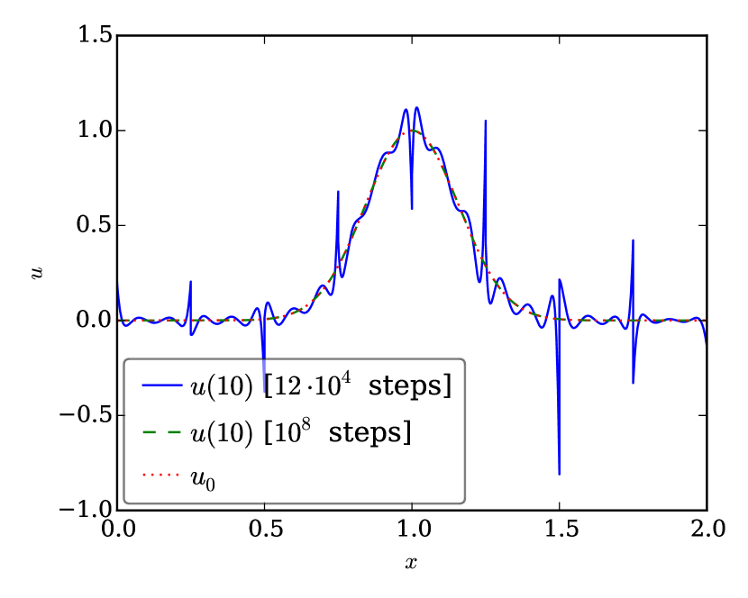
(a) Solution computed without additional artificial dissipation.

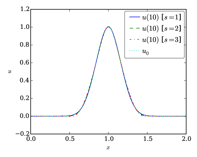
(b) Solution computed using adaptive artificial dissipation.

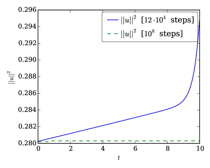
(c) Energy of the solution computed without additional artificial dissipation.

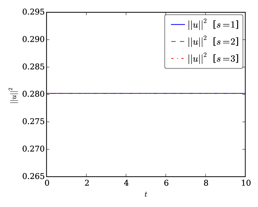
(d) Energy of the solution computed using adaptive artificial dissipation.

Figure 1: Numerical results for linear advection using $N=8$ elements with polynomials of degree $\leq p=7$. On the left hand side, no additional artificial dissipation has been used, whereas adaptive spectral viscosity of orders $s=1$, $s=2$, and $s=3$ has been used for the right hand side.

As can be seen in Figure 1(c), the energy of the solution using $12\cdot 10^{4}$ time steps is increasing, as expected. This yields undesired oscillations in Figure 1(a). However, increasing the number of time steps to $10^{8}$ reduces the additional term of order $(\Delta t)^{2}$. Therefore, the energy does not increase that much and the solution has the desired smooth form.

However, the same effect can be achieved by adaptive artificial dissipation using the estimate for the strength $\varepsilon$ of Lemma 3. Using orders $s\in\mathinner{\left\{1,2,3\right\}}$, the energy in Figure 1(d) remains constant and the solutions in Figure 1(b) look as expected. However, there is a slight perturbation for $s=3$ around $x\approx 1\pm 0.5$.

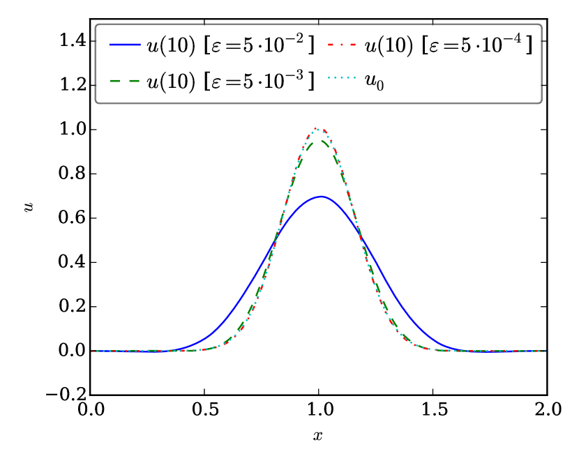
(a) Solutions for order $s=1$.

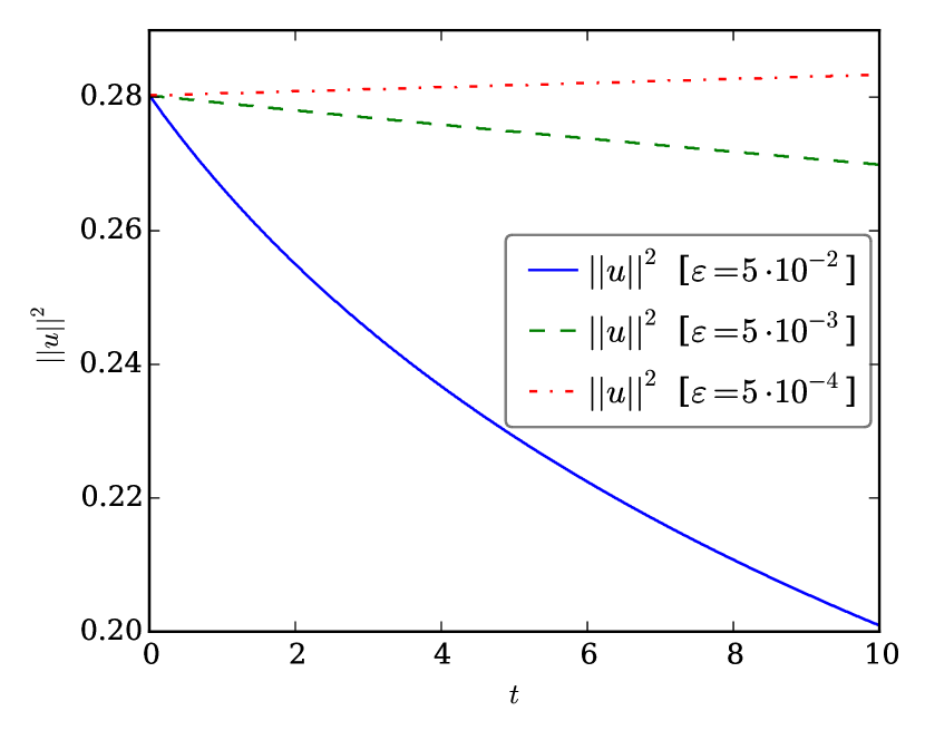
(b) Energies for order $s=1$.

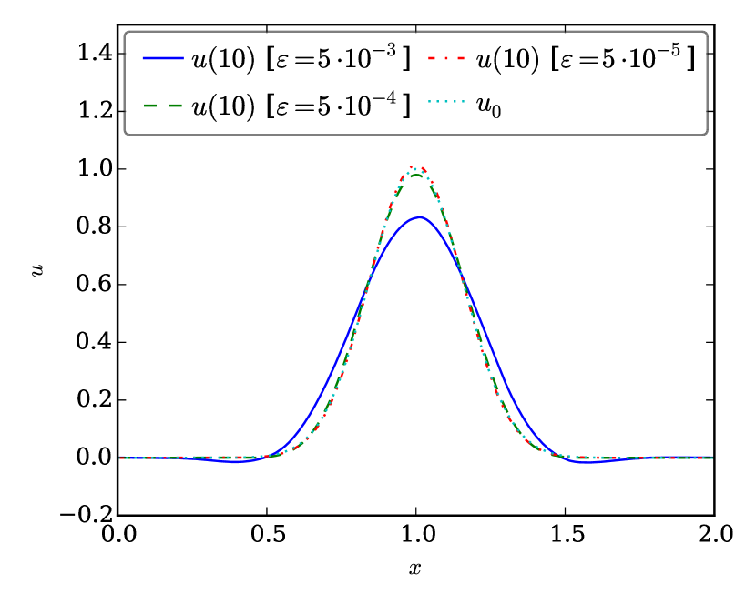
(c) Solutions for order $s=2$.

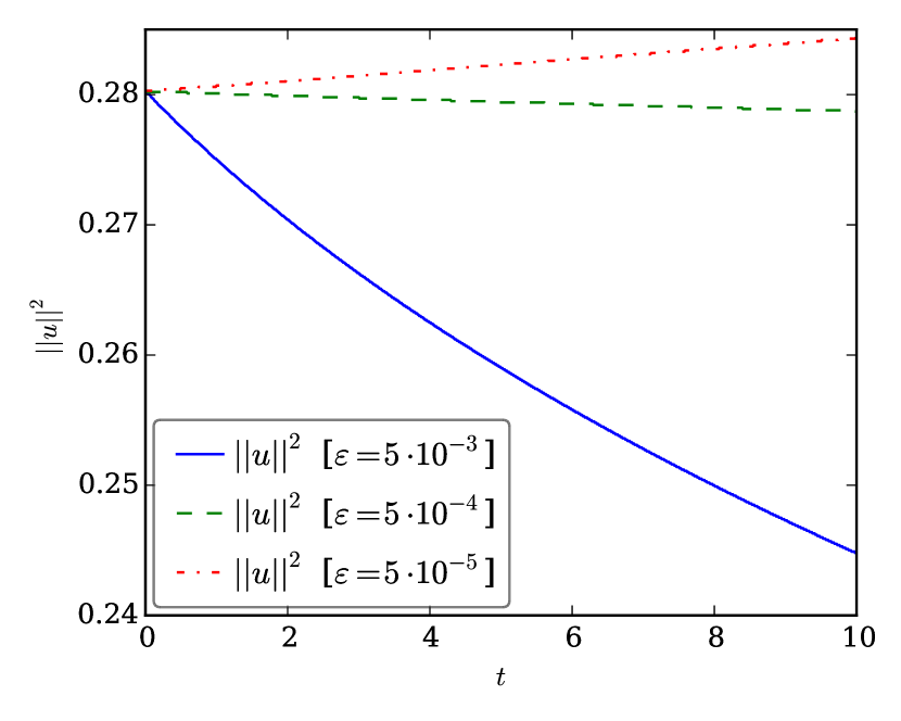
(d) Energies for order $s=2$.

Figure 2: Numerical results for linear advection using $N=8$ elements with polynomials of degree $\leq p=7$ and constant artificial dissipation of orders $s\in\mathinner{\left\{1,2\right\}}$ with various strengths $\varepsilon$. On the left hand side, the solutions $u$ are shown, accompanied by the corresponding energies $\mathinner{\!\left\lVert u\right\rVert}^{2}$ on the right hand side.

As can be seen in Figure 2, simple artificial dissipation of fixed strength $\varepsilon$ has a stabilising effect. The dissipation of energy $\mathinner{\!\left\lVert u\right\rVert}^{2}$ is increasing with increasing order $s$ and strength $\varepsilon$, respectively. However, to get an acceptable result requires lengthy experiments and fine tuning of the parameters by hand. Therefore, the adaptive strategy of Lemma 3 provides an excellent alternative.

4.2 Linear advection with discontinuous initial condition

In order to see the influence in the presence of discontinuities, the linear advection equation (9)

$$\partial_{t}u+\partial_{x}u=0,\qquad u(0,x)=u_{0}(x)=\begin{cases}1,&x\in[0.5,1],\\ 0,&\text{otherwise},\end{cases}$$ (70)

with periodic boundaries in the domain $[0,2]$ has been investigated during the time interval $[0,8]$. The semidiscretisation (10) is used with an upwind numerical flux $f^{\mathrm{num}}(u_{-},u_{+})=u_{-}$ and rendered fully discrete by an explicit Euler method.

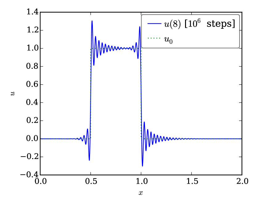
(a) Solution computed without additional artificial dissipation.

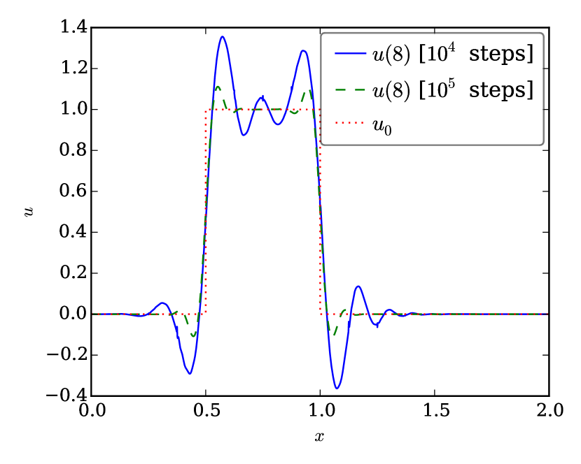
(b) Solution computed using adaptive artificial dissipation.

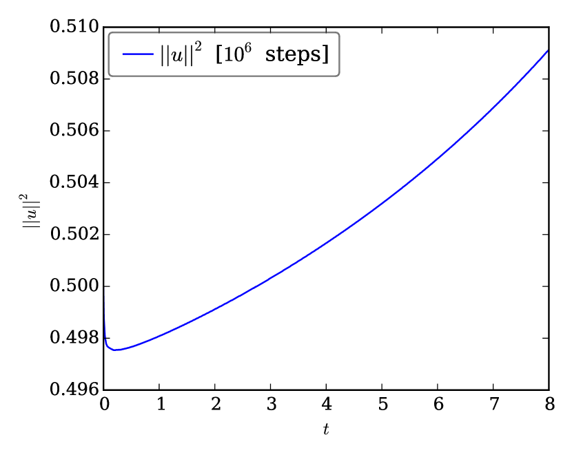
(c) Energy of the solution computed without additional artificial dissipation.

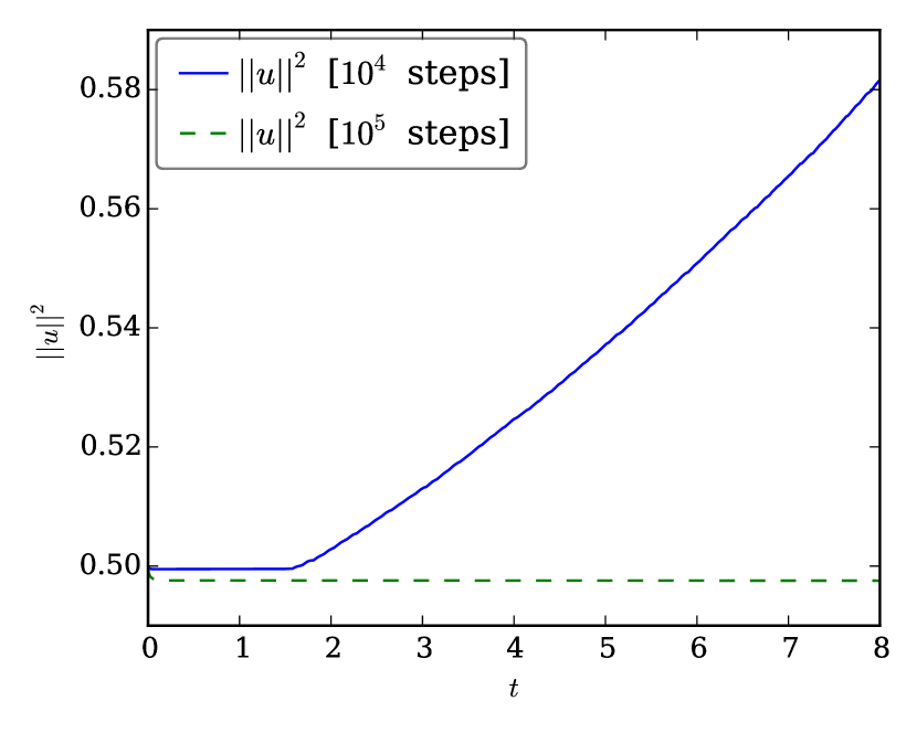
(d) Energy of the solution computed using adaptive artificial dissipation.

Figure 3: Numerical results for linear advection using $N=16$ elements with polynomials of degree $\leq p=15$. On the left hand side, no additional artificial dissipation has been used, whereas adaptive spectral viscosity of orders $s=1$ has been used for the right hand side.

Using $10^{6}$ time steps, the energy of the solution computed without artificial dissipation increases, as can be seen in Figure 3(c). Additionally, Figure 3(a) shows dominant oscillations that have been developed. Contrary, adaptive artificial dissipation stabilises the scheme. Therefore, $10^{4}$ time steps suffice to get a bounded increase in the energy and some oscillations, see Figures 3(d) and 3(b). With the same number of time steps, the computation without spectral viscosity blows up. However, the artificial dissipation operator introduces a restriction on the possible time steps. Thus, if the time step is too big, the desired estimate on the strength $\varepsilon$ fails. Setting $\varepsilon$ to zero in this case is the best possible solution, but the energy might increase. This phenomenon is visible in Figure 3(d). Increasing the number of time steps to $10^{5}$ yields the desired constant energy and less oscillations in the solution plotted in Figure 3(b).

4.3 Burgers’ equation

Burgers’ equation (11) with smooth initial condition

$$\partial_{t}u+\partial_{x}\frac{u^{2}}{2}=0,\quad u(0,x)=u_{0}(x)=\sin\pi x+0.01$$ (71)

in the periodic domain $[0,2]$ is used as a prototypical example of a nonlinear conservation law yielding a discontinuous solution in finite time $t\in[0,3]$. The stable semidiscretisation (13) with $N=16$ elements representing polynomials of degree $\leq p=16$ in nodal Gauß-Legendre bases is used with the local Lax-Friedrichs flux $f^{\mathrm{num}}(u_{-},u_{+})=\frac{u_{-}^{2}+u_{+}^{2}}{4}-\frac{\max\mathinner{\left\{\mathinner{\!\left\lvert u_{-}\right\rvert},\mathinner{\!\left\lvert u_{+}\right\rvert}\right\}}}{2}(u_{+}-u_{-})$. The explicit Euler method as time integrator uses $15\cdot 10^{3}$ steps for the interval $[0,3]$.

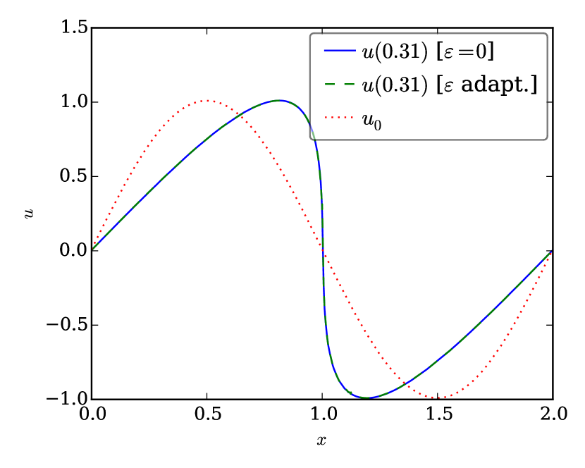
(a) Solution at time $t=0.31$.

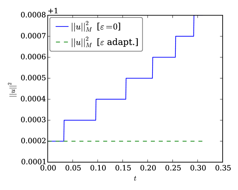
(b) Energy in the time interval $[0,0.31]$.

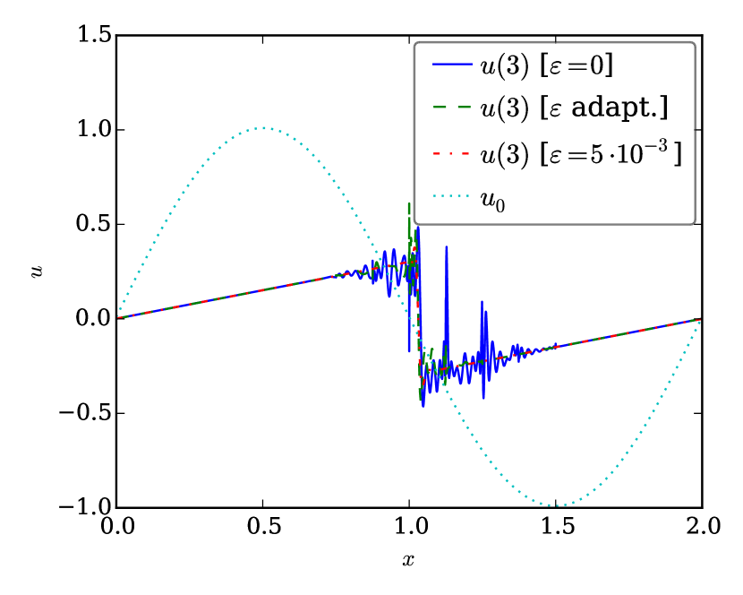
(c) Solution at time $t=3$.

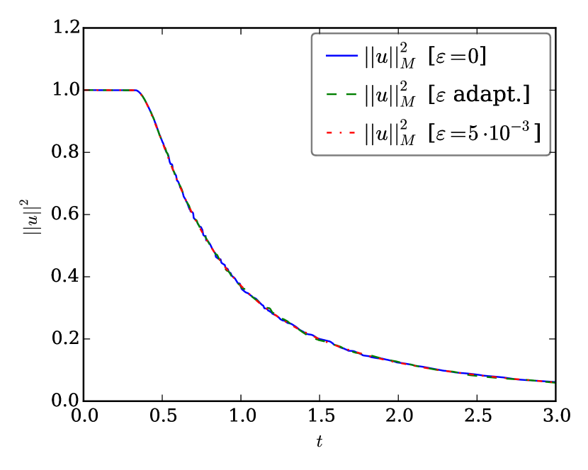
(d) Energy in the time interval $[0,3]$.

Figure 4: Numerical results for Burgers’ equation using $N=16$ elements with polynomials of degree $\leq p=15$. The solutions and the energy are plotted on the left hand side and right hand side, respectively.

At time $t=0.31$, the solution in Figure 4(a) computed with only $500$ time steps is still smooth. However, the energy in Figure 4(b) increases if no artificial dissipation is used. Contrary applying adaptive spectral viscosity results in a constant energy.

At time $t=3$, the solution in Figure 4(c) has developed a discontinuity resulting in oscillations around $x\approx 1$. Although adaptive artificial dissipation damps these a bit, it does not removed them. However, spectral viscosity of fixed strength $\varepsilon=5\cdot 10^{-3}$ adds enough dissipation to remove them and yields a non-oscillatory result. Nevertheless, all three choices of spectral viscosity yield nearly visually indistinguishable results for the energy in Figure 4(d) due to the dissipative numerical flux.

5 Conclusions and further research

In this work, artificial dissipation / spectral viscosity has been considered in the general framework of CPR methods using SBP operators. A naive discretisation of the viscosity operator does not yield the desired results, whereas the chosen representation (after the application of summation-by-parts and cancellation of undesired boundary terms) results in the estimates expected from the continuous setting.

Additionally, a new adaptive strategy has been proposed in order to compute the strength of the viscosity in a way to get a stable fully discrete scheme obtained by an explicit Euler method. Thus, additional terms of order $(\Delta t)^{2}$ that appear in the estimate of the energy growth in one time step are compensated. However, this artificial dissipation is not enough to remove all oscillations, especially the ones developing in nonlinear problems.

Numerical results for linear advection and Burgers’ equation have been presented, showing the advantages of the chosen approach as well as some limitations. The application of artificial dissipation stabilises the scheme, but also introduces additional restrictions on the time step. Therefore, removing these by an operator splitting approach is desired and conducted in the second part of this series by [5].

Another topic of further research is the investigation of different time integration methods. While strong-stability preserving (SSP) schemes can be written as convex combinations of explicit Euler steps and inherit therefore the stability properties, other adaptive strategies might be advantageous in this setting.

Moreover, extending the approach to other hyperbolic conservation laws will be interesting.

6 Appendix: Legendre polynomials

The Legendre polynomials can be represented by Rodrigues’ formula (equation 8.6.18 of [1])

$$\varphi_{p}(x)=\frac{1}{2^{p}\,p!}\dfrac{\operatorname{d\!}{{}^{p}}}{\operatorname{d\!}{x^{p}}}(x^{2}-1)^{p}$$ (72)

and are orthogonal in $L_{2}[-1,1]$ with $\mathinner{\!\left\lVert\varphi_{p}\right\rVert}^{2}=2/(2p+1)$. Their boundary values are $\varphi_{p}(1)=1$ and $\varphi_{p}(-1)=(-1)^{p}$. Due to Rodrigues’ formula, they are symmetric for even $p$ and antisymmetric for odd $p$. Additionally, they obey

$$\varphi_{p+1}^{\prime}(x) =\frac{1}{2^{p+1}\,(p+1)!}\dfrac{\operatorname{d\!}{{}^{p+2}}}{\operatorname{d\!}{x^{p+2}}}(x^{2}-1)^{p+1}$$ (73)

$$=\frac{1}{2^{p+1}\,(p+1)!}\dfrac{\operatorname{d\!}{{}^{p+1}}}{\operatorname{d\!}{x^{p+1}}}\left[2(p+1)x(x^{2}-1)^{p}\right]$$

$$=\frac{1}{2^{p}\,p!}\dfrac{\operatorname{d\!}{{}^{p}}}{\operatorname{d\!}{x^{p}}}\dfrac{\operatorname{d\!}{}}{\operatorname{d\!}{x}}\left[x(x^{2}-1)^{p}\right]$$

$$=\frac{1}{2^{p}\,p!}\dfrac{\operatorname{d\!}{{}^{p}}}{\operatorname{d\!}{x^{p}}}\left[(x^{2}-1)^{p}+2px^{2}(x^{2}-1)^{p-1}\right]$$

$$=\frac{1}{2^{p}\,p!}\dfrac{\operatorname{d\!}{{}^{p}}}{\operatorname{d\!}{x^{p}}}\left[(2p+1)(x^{2}-1)^{p}+2p(x^{2}-1)^{p-1}\right]$$

$$=(2p+1)\frac{1}{2^{p}\,p!}\dfrac{\operatorname{d\!}{{}^{p}}}{\operatorname{d\!}{x^{p}}}(x^{2}-1)^{p}+\frac{1}{2^{p-1}\,(p-1)!}\dfrac{\operatorname{d\!}{{}^{p}}}{\operatorname{d\!}{x^{p}}}(x^{2}-1)^{p-1}$$

$$=(2p+1)\varphi_{p}(x)+\varphi_{p-1}^{\prime}(x).$$

The first three Legendre polynomials are $\varphi_{0}(x)=1$, $\varphi_{1}(x)=x$, $\varphi_{2}(x)=(3x^{2}-1)/2$.

In order to compute the $L_{2}$ projection of $(1-x^{2})\varphi_{p}(x)$ on the space of polynomials of degree $\leq p$, equation 8.5.4 of [1] can be used

$$(x^{2}-1)\partial_{x}\varphi_{p}(x)=px\varphi_{p}(x)-p\varphi_{p-1}(x).$$ (74)

Inserting equation 8.5.3 of [1]

$$(p+1)\varphi_{p+1}(x)=(2p+1)x\varphi_{p}(x)-p\varphi_{p-1}(x)$$ (75)

results in

$$(x^{2}-1)\partial_{x}\varphi_{p}(x) =\frac{p(p+1)}{2p+1}\varphi_{p+1}+\frac{p^{2}}{2p+1}\varphi_{p-1}(x)-p\varphi_{p-1}(x)$$ (76)

$$=\frac{p(p+1)}{2p+1}\varphi_{p+1}(x)-\frac{p(p+1)}{2p+1}\varphi_{p-1}(x).$$

The Lobatto-Legendre quadrature includes both boundary nodes and is exact for polynomials of degree $\leq 2p-1$. The norm of $\varphi_{p}$, evaluated by Lobatto-Legendre quadrature is (equation (1.136) of [12])

$$\mathinner{\!\left\lVert\underline{\varphi}_{p}\right\rVert}_{M}^{2}=\underline{\varphi}_{p}^{T}\underline{\underline{M}}\,\underline{\varphi}_{p}=\frac{2}{p}.$$ (77)

In order to compute $\underline{\varphi}_{p-1}^{T}\underline{\underline{M}}\,\underline{\varphi}_{p+1}$ via Lobatto-Legendre quadrature, the product can be expanded as a linear combination of Legendre polynomials

$$\varphi_{p-1}\varphi_{p+1}=\sum_{n=0}^{2p}\beta_{n}\varphi_{n}.$$ (78)

Since the Legendre polynomials are orthogonal, $\beta_{0}=0$. As used by [23], the leading coefficient of the Legendre polynomial $\varphi_{n}$ of degree $n$ is

$$a_{n}=\frac{(2n)!}{2^{n}(n!)^{2}}.$$ (79)

Thus,

$$\beta_{2p} =\frac{a_{p-1}a_{p+1}}{a_{2p}}=\frac{(2p-2)!}{2^{p-1}((p-1)!)^{2}}\frac{(2p+2)!}{2^{p+1}((p+1)!)^{2}}\frac{2^{2p}((2p)!)^{2}}{(4p)!}$$ (80)

$$=\frac{(2p-2)!\,(2p+2)!\,((2p)!)^{2}}{((p-1)!)^{2}\,((p+1)!)^{2}\,(4p)!}.$$

Denoting the approximation of $\int\cdot$ by Lobatto-Legendre quadrature as $\int_{L}\cdot$, $\int_{L}\varphi_{2p}$ has to be computed. To use equation (77), $\varphi_{p}^{2}$ is expanded similar to $\varphi_{p-1}\varphi_{p+1}$

$$\varphi_{p}^{2}=\sum_{n=0}^{2p}\gamma_{n}\varphi_{n}.$$ (81)

Since Legendre polynomials are orthogonal,

$$\gamma_{0}=\mathinner{\!\left\lVert\varphi_{p}\right\rVert}^{2}/\int\varphi_{0}=\frac{1}{2p+1}.$$ (82)

Similar to $\beta_{2p}$, $\gamma_{2p}$ can be written as

$$\gamma_{2p}=\frac{a_{p}^{2}}{a_{2p}}=\frac{\left[(2p)!\right]^{2}}{2^{2p}(p!)^{4}}\frac{2^{2p}((2p)!)^{2}}{(4p)!}=\frac{\left[(2p)!\right]^{4}}{(p!)^{4}\,(4p)!}.$$ (83)

Using $\int_{L}\varphi_{p}^{2}=2/p$ from equation (77) and linearity of the quadrature yields

$$\frac{2}{p}=\int_{L}\varphi_{p}^{2}=\sum_{n=0}^{2p}\gamma_{n}\int\varphi_{n}=\gamma_{0}\int_{L}\varphi_{0}+\gamma_{2p}\int_{L}\varphi_{2p}=2\gamma_{0}+\gamma_{2p}\int_{L}\varphi_{2p},$$ (84)

since the quadrature is exact (and thus zero) for $\varphi_{n},n\in\mathinner{\left\{1,\dots,2p-1\right\}}$. Therefore,

$$\int_{L}\varphi_{2p}=\left(\frac{2}{p}-2\gamma_{0}\right)\gamma_{2p}^{-1}=\left(\frac{2}{p}-\frac{2}{2p+1}\right)\gamma_{2p}^{-1}=2\frac{p+1}{p(2p+1)}\frac{(p!)^{4}\,(4p)!}{\left[(2p)!\right]^{4}}.$$ (85)

Finally, using $\beta_{0}=0$ and $\int_{L}\varphi_{n}=0$ for $n\in\mathinner{\left\{1,\dots,2p-1\right\}}$,

$$\underline{\varphi}_{p-1}^{T}\underline{\underline{M}}\,\underline{\varphi}_{p+1} =\int_{L}\varphi_{p-1}\varphi_{p+1}=\sum_{n=0}^{2p}\beta_{n}\int_{L}\varphi_{n}=\beta_{2p}\int_{L}\varphi_{2p}$$ (86)

$$=\frac{(2p-2)!\,(2p+2)!\,((2p)!)^{2}}{((p-1)!)^{2}\,((p+1)!)^{2}\,(4p)!}\cdot 2\frac{p+1}{p(2p+1)}\frac{(p!)^{4}\,(4p)!}{\left[(2p)!\right]^{4}}$$

$$=\frac{2}{p}\frac{p+1}{2p+1}\frac{(p!)^{2}}{((p-1)!)^{2}}\frac{(p!)^{2}}{((p+1)!)^{2}}\frac{(2p-2)!}{(2p)!}\frac{(2p+2)!}{(2p)!}$$

$$=\frac{2}{p}\frac{p+1}{2p+1}\frac{p^{2}}{1}\frac{1}{(p+1)^{2}}\frac{1}{2p(2p-1)}\frac{(2p+2)(2p+1)}{1}$$

$$=\frac{2}{p}\frac{p}{2p-1}.$$

References

- [1] Milton Abramowitz and Itene A Stegun “Handbook of mathematical functions” National Bureau of Standards, 1972
- [2] David C Del Rey Fernández, Pieter D Boom and David W Zingg “A generalized framework for nodal first derivative summation-by-parts operators” In Journal of Computational Physics 266 Elsevier, 2014, pp. 214–239
- [3] David C Del Rey Fernández, Jason E Hicken and David W Zingg “Review of summation-by-parts operators with simultaneous approximation terms for the numerical solution of partial differential equations” In Computers & Fluids 95 Elsevier, 2014, pp. 171–196
- [4] Gregor J Gassner “A skew-symmetric discontinuous Galerkin spectral element discretization and its relation to SBP-SAT finite difference methods” In SIAM Journal on Scientific Computing 35.3 SIAM, 2013, pp. A1233–A1253
- [5] Jan Glaubitz, Hendrik Ranocha, Philipp Öffner and Thomas Sonar “Enhancing stability of correction procedure via reconstruction using summation-by-parts operators II: Modal filtering” Submitted, 2016
- [6] Sigal Gottlieb, David I Ketcheson and Chi-Wang Shu “Strong stability preserving Runge-Kutta and multistep time discretizations” World Scientific, 2011
- [7] Jason E Hicken, David C Del Rey Fernández and David W Zingg “Multidimensional Summation-By-Parts Operators: General Theory and Application to Simplex Elements”, 2015 arXiv:1505.03125 [math.NA]
- [8] HT Huynh “A flux reconstruction approach to high-order schemes including discontinuous Galerkin methods” In AIAA paper 4079, 2007, pp. 2007
- [9] HT Huynh, Zhi J Wang and Peter E Vincent “High-order methods for computational fluid dynamics: A brief review of compact differential formulations on unstructured grids” In Computers & Fluids 98 Elsevier, 2014, pp. 209–220
- [10] Antony Jameson “A proof of the stability of the spectral difference method for all orders of accuracy” In Journal of Scientific Computing 45.1-3 Springer, 2010, pp. 348–358
- [11] Antony Jameson, Peter E Vincent and Patrice Castonguay “On the non-linear stability of flux reconstruction schemes” In Journal of Scientific Computing 50.2 Springer, 2012, pp. 434–445
- [12] David A Kopriva “Implementing spectral methods for partial differential equations: Algorithms for scientists and engineers” Springer Science & Business Media, 2009
- [13] Heping Ma “Chebyshev–Legendre Spectral Viscosity Method for Nonlinear Conservation Laws” In SIAM Journal on Numerical Analysis 35.3 SIAM, 1998, pp. 869–892
- [14] Heping Ma “Chebyshev–Legendre Super Spectral Viscosity Method for Nonlinear Conservation Laws” In SIAM Journal on Numerical Analysis 35.3 SIAM, 1998, pp. 893–908
- [15] Ken Mattsson, Magnus Svärd and Jan Nordström “Stable and accurate artificial dissipation” In Journal of Scientific Computing 21.1 Springer, 2004, pp. 57–79
- [16] Jan Nordström “Conservative finite difference formulations, variable coefficients, energy estimates and artificial dissipation” In Journal of Scientific Computing 29.3 Springer, 2006, pp. 375–404
- [17] Jan Nordström and Peter Eliasson “New developments for increased performance of the SBP-SAT finite difference technique” In IDIHOM: Industrialization of High-Order Methods-A Top-Down Approach Springer, 2015, pp. 467–488
- [18] Hendrik Ranocha “SBP operators for CPR methods”, 2016 URL: http://www.digibib.tu-bs.de/?docid=00063111
- [19] Hendrik Ranocha, Philipp Öffner and Thomas Sonar “Extended skew-symmetric form for summation-by-parts operators” Submitted, 2015 arXiv:1511.08408 [math.NA]
- [20] Hendrik Ranocha, Philipp Öffner and Thomas Sonar “Summation-by-parts operators for correction procedure via reconstruction” In Journal of Computational Physics 311 Elsevier, 2016, pp. 299–328 DOI: 10.1016/j.jcp.2016.02.009
- [21] Magnus Svärd and Jan Nordström “Review of summation-by-parts schemes for initial-boundary-value problems” In Journal of Computational Physics 268 Elsevier, 2014, pp. 17–38
- [22] Eitan Tadmor “Convergence of spectral methods for nonlinear conservation laws” In SIAM Journal on Numerical Analysis 26.1 SIAM, 1989, pp. 30–44
- [23] Peter E Vincent, Patrice Castonguay and Antony Jameson “A new class of high-order energy stable flux reconstruction schemes” In Journal of Scientific Computing 47.1 Springer, 2011, pp. 50–72
- [24] Peter E Vincent, Antony M Farrington, Freddie D Witherden and Antony Jameson “An extended range of stable-symmetric-conservative Flux Reconstruction correction functions” In Computer Methods in Applied Mechanics and Engineering 296 Elsevier, 2015, pp. 248–272
- [25] John von Neumann and Robert D Richtmyer “A method for the numerical calculation of hydrodynamic shocks” In Journal of Applied Physics 21.3 AIP Publishing, 1950, pp. 232–237
- [26] Freddie D Witherden and Peter E Vincent “An analysis of solution point coordinates for flux reconstruction schemes on triangular elements” In Journal of Scientific Computing 61.2 Springer, 2014, pp. 398–423