Fast Bayesian Whole-Brain fMRI Analysis with Spatial 3D Priors

Abstract.

Spatial whole-brain Bayesian modeling of task-related functional magnetic resonance imaging (fMRI) is a great computational challenge. Most of the currently proposed methods therefore do inference in subregions of the brain separately or do approximate inference without comparison to the true posterior distribution. A popular such method, which is now the standard method for Bayesian single subject analysis in the SPM software, is introduced in Penny et al., 2005b . The method processes the data slice-by-slice and uses an approximate variational Bayes (VB) estimation algorithm that enforces posterior independence between activity coefficients in different voxels. We introduce a fast and practical Markov chain Monte Carlo (MCMC) scheme for exact inference in the same model, both slice-wise and for the whole brain using a 3D prior on activity coefficients. The algorithm exploits sparsity and uses modern techniques for efficient sampling from high-dimensional Gaussian distributions, leading to speed-ups without which MCMC would not be a practical option. Using MCMC, we are for the first time able to evaluate the approximate VB posterior against the exact MCMC posterior, and show that VB can lead to spurious activation. In addition, we develop an improved VB method that drops the assumption of independent voxels a posteriori. This algorithm is shown to be much faster than both MCMC and the original VB for large datasets, with negligible error compared to the MCMC posterior.

1. Introduction

Over the past fifteen years, there has been much work devoted to Bayesian spatial modeling of task-related functional magnetic resonance imaging (fMRI) data. The motivation to this line of work has been to develop an extension to the classical general linear model (GLM) approach (Friston et al.,, 1995). The idea is to replace pre-smoothing of data and post-correction of multiple hypothesis testing – an approach that was recently shown to be problematic for cluster inference (Eklund et al.,, 2016) – with a proper spatial model. A corner stone in the field is a series of papers (Penny et al.,, 2003; Penny et al., 2005a, ; Penny et al., 2005b, ; Penny et al.,, 2007; Penny and Flandin,, 2005) upon which the Bayesian spatial single-subject analysis method in the Statistical Parametric Mapping (SPM) software (SPM,, 2002) is built. The method extends the classical GLM approach to a Bayesian framework with a spatial Gaussian Markov Random Field (GMRF) prior on the activity parameters and the temporal noise parameters, encouraging them to vary smoothly across the brain. The prior is formulated such that the optimal amount of smoothness can be estimated from the data. A fast variational Bayes (VB) algorithm is used for inference, but makes the assumptions that (i) the posterior factorizes over different types of parameters and (ii) the posterior for the activity parameters and the temporal noise model parameters factorizes over voxels. Assumption (i) is validated in the univariate (single-voxel) case in Penny et al., (2003) by comparing the VB posterior to the exact posterior obtained from MCMC sampling, but the error from assumption (ii) has to our knowledge never been properly examined. The VB framework also allows Bayesian model comparison based on the model evidence lower bound (Penny et al.,, 2007), but the computation of determinants of spatial precision matrices limits these types of analyses to be performed slice by slice or to sub-volumes containing $\apprle 10000$ voxels. Even without the model comparison, the SPM method would be considered too time consuming for the full 3D brain analysis for most practitioners.

A number of extensions of the SPM method have been developed. Harrison et al., 2008a replace the stationary spatial prior in Penny et al., 2005b with a non-stationary prior which is more adaptive and find evidence for this in data from an fMRI study of the auditory system. Groves et al., (2009) note that the spatial prior in Penny et al., 2005b actually performs simultaneous smoothing and shrinkage of activity parameters in a rather non-flexible way. They separate these two effects using a Gaussian Process (GP) prior with a squared exponential kernel function, and infer the kernel length scale using Evidence Optimization (EO). The same issue is targeted in Yue et al., (2014), who use the GMRF representation of a Matérn field (Lindgren et al.,, 2011) and perform estimation using Integrated Nested Laplace Approximation (INLA) (Rue et al.,, 2009).

Even though all of these extensions seem like improvements from a modeling perspective they all struggle with computational complexity and inference is only performed slice by slice. A computationally attractive approach towards spatial 3D modeling is to first partition the brain into sub-volumes or parcels (Thirion et al.,, 2014), and then estimate a separate 3D model for each parcel, which can also be done in parallel, see for example Harrison et al., 2008b ; Vincent et al., (2010); Musgrove et al., (2016). The inability to model dependencies between parcels is a bit unnatural, however, and Harrison et al., 2008b notice discontinuities in posterior estimates along partition boundaries when using their model. Full 3D brain analysis with reasonable speed is achieved by Harrison and Green, (2010) who approximate the zero mean spatial prior in Penny et al., 2005b with a non-zero mean empirical prior, with the cost of no longer having a true generative model.

An alternative route to a spatial model is to view selecting active voxels as a variable selection problem, with a spatial prior on the probability of activation in a certain voxel, see for example Smith and Fahrmeir, (2007) and Zhang et al., (2014). A comparison between estimation by VB and MCMC for this kind of model is available in the recent paper by Zhang et al., (2016). In a related line of work (Vincent et al.,, 2010; Risser et al.,, 2011; Chaari et al.,, 2013), voxel activations are modeled using a spatial mixture model of Gaussian distributions, where one of the mixture components has mean zero, corresponding to non-active voxels. This framework has the benefit of allowing for simultaneous estimation of the hemodynamic response function (HRF), using both MCMC and variational methods which are applied parcel-wise. Another possibility is to model not only the activity parameters, but also the noise as spatially dependent (see for example Woolrich et al., (2004)), an assumption that seems natural but which comes with computational trouble because of the spatio-temporal structure.

A typical goal with these types of analyses is to compute Posterior Probability Maps (PPMs) (Friston and Penny,, 2003), that is, brain maps showing the marginal probability of activation under a certain stimuli in each voxel. It is also common that these PPMs are thresholded at some level, for example at $p>0.9$, to display active voxels or regions. However, such thresholding implicitly defines a hypothesis test in each voxel and these multiple tests must be corrected for. Given a spatially dependent posterior, a natural way to do this is using theory on excursion sets (Bolin and Lindgren,, 2015) as in Yue et al., (2014) who define the term joint PPM based on the joint posterior, as opposed to marginal PPMs.

Our paper makes a number of contributions. First, we propose a fast and practical MCMC algorithm for slice-by-slice and whole brain task-fMRI analysis with spatial priors on the activity fields and the autoregressive noise parameters. The algorithm makes efficient use of sparsity and sampling from high-dimensional Gaussian distributions using preconditioned conjugate gradient (PCG) methods. These efficiency improvements reduce the computational complexity by several orders of magnitude. Collectively, they make it possible to perform posterior whole-brain analysis with spatial priors on problems where MCMC was previously simply not a practical option. Second, we develop a very fast VB approach that maintains the weaker independence assumption (i) in SPM’s VB method, but drops the stronger assumption (ii). Letting go of the assumption of spatially a posteriori independent voxels is non-trivial from a computational standpoint, and we employ several numerical techniques that together make the non-factorized VB approximation a very fast alternative to MCMC. The approximation errors from this non-factorized VB are shown to be essentially negligible for practical applications. Third, we demonstrate that the completely factorized VB in SPM12 can lead to spurious activations via a hitherto unexplored channel. Factorized VBs are well known to underestimate posterior variances, but we highlight and explain why the factorization over voxels can also result in a quite distorted smoothing of the activations.

The paper is organized as follows. We give a short background on the spatial model in SPM and the VB method used there to estimate the model. We then introduce the MCMC algorithm and the improved VB method and put extra emphasis on how to make these methods computationally efficient. In the next section we show results for simulated and real experiment data, and illustrate how the parameter estimates and PPMs differ between the different methods. The speed and convergence properties across methods are also compared. The last section contains a discussion and our conclusions. Derivation of results and implementation details can be found in the appendices.

The new methods presented in this article have been implemented as an extension to the SPM software, available at http://www.fil.ion.ucl.ac.uk/spm/ext/#BFAST3D.

2. Background

We will consider single-subject fMRI-data containing $T$ volumes with $N$ voxels ordered in a $T\times N$ matrix $\mathbf{Y}$. The experiment is described by the $T\times K$ design matrix $\mathbf{X}$, with $K$ regressors. The model in Penny et al., (2007) is written as

$$\mathbf{Y}=\mathbf{X}\mathbf{W}+\mathbf{E},$$ (2.1)

where $\mathbf{W}$ is a $K\times N$ matrix of regression coefficients and $\mathbf{E}$ is a $T\times N$ matrix of error terms. Since this is the same model that will be considered here, we will use the same notation throughout, unless stated otherwise. Voxel-specific, normally distributed $P$th order AR models are assumed for the error terms, but for a clearer presentation here we will consider the special case $P=0$ and handle the more general case in Appendix A. The likelihood then becomes

$$p\left(\mathbf{Y}|\mathbf{W},\boldsymbol{\lambda}\right) = \prod_{n=1}^{N}\mathcal{N}\left(\mathbf{Y}_{\cdot,n};\mathbf{X}\mathbf{W}_{\cdot,n},\lambda_{n}^{-1}\mathbf{I}_{T}\right),$$ (2.2)

with $\mathbf{Y}_{\cdot,n}$ and $\mathbf{W}_{\cdot,n}$ denoting the $n$th column of $\mathbf{Y}$ and $\mathbf{W},$ $\lambda_{n}$ as the noise precision of voxel $n$ and $\mathbf{I}_{T}$ a $T\times T$ identity matrix. The likelihood factorizes over voxels, which is an assumption of non-spatial measurement noise that is made because the opposite assumption would be very computationally challenging. Instead, the spatial part of the model will enter via the prior on the regression coefficients

$$\mathbf{W}_{k,\cdot}^{\prime}|\alpha_{k} \sim \mathcal{N}\left(0,\alpha_{k}^{-1}\mathbf{D}_{w}^{-1}\right),$$ (2.3)

$$p\left(\mathbf{W}|\boldsymbol{\alpha}\right) = \prod_{k=1}^{K}p\left(\mathbf{W}_{k,\cdot}^{\prime}|\alpha_{k}\right),$$

where $\mathbf{W}_{k,\cdot}^{\prime}$ denotes the transposed $k$th row of $\mathbf{W}$, $\mathbf{D}_{w}$ is a fixed spatial $N\times N$ precision matrix and $\boldsymbol{\alpha}=\left(\alpha_{1},\ldots,\alpha_{K}\right)^{\prime}$ are hyperparameters to be estimated from the data. There are several possible choices for $\mathbf{D}_{w}$, but we will here focus on the SPM12 default choice, the unweighted graph-Laplacian (UGL) (called $\mathbf{L}$ in Penny et al., 2005b ) which for each voxel has the number of adjacent voxels on the diagonal and $\mathbf{D}_{w}(i,j)=-1$ if $i$ and $j$ are adjacent. For voxels in the interior part of the brain we will thus have $6$’s on the diagonal when modeling the whole 3D brain, and $4$’s when modeling each 2D slice separately. The main focus in Penny et al., 2005b is on a different prior defined as $\mathbf{D}_{w}=\mathbf{L}^{\prime}\mathbf{L}$. It is straightforward to use that prior also in our framework, but our experience is that it leads to too smooth posteriors, which is probably the reason why it is not the default option in SPM12. It also leads to slower inference since $\mathbf{D}_{w}$ is less sparse when using this prior. The assumption of a sparse $\mathbf{D}_{w}$ is the key to fast inference for this type of model using any method.

The hyperparameter $\alpha_{k}$ will be estimated for each regressor to put the appropriate weight on the prior, depending on what smoothness is supported by the data. A higher $\alpha_{k}$ brings the regression coefficient in each voxel closer to the mean of the coefficients in neighboring voxels (more smoothness), and globally all coefficients closer to zero (more shrinkage). The precision parameters $\alpha_{k}$ and $\lambda_{n}$ are assigned conjugate Gamma priors. For all the details on the generative model and the priors, see Figure 1 and Appendix A in Penny et al., (2007) which also gives the values of the prior parameters that are default in SPM12 which are also used here (except $r_{1}=10000$ in SPM12). That is, we use $q_{1}=u_{1}=10$, $r_{1}=10000$ and $q_{2}=r_{2}=u_{2}=0.1$.

The VB algorithm for inference presented in Penny et al., 2005b makes two independence assumptions for the joint posterior distribution. Firstly, the posterior is assumed to factorize over the different kinds of parameters, that is

$$q\left(\mathbf{W},\boldsymbol{\alpha},\boldsymbol{\lambda}|\mathbf{Y}\right)=q\left(\mathbf{W}|\mathbf{Y}\right)q\left(\boldsymbol{\alpha}|\mathbf{Y}\right)q\left(\boldsymbol{\lambda}|\mathbf{Y}\right),$$ (2.4)

with $q$ denoting VB posteriors. Secondly, the regression parameters (and the AR-parameters in the general case) are assumed to factorize over voxels

$$q\left(\mathbf{W}|\mathbf{Y}\right)=\prod_{n=1}^{N}q\left(\mathbf{W}_{\cdot,n}|\mathbf{Y}\right).$$ (2.5)

The second assumption is possibly the strongest and most counter-intuitive since it is clear that the spatial prior will generate dependence between voxels in the posterior. In the following section we will present an efficient MCMC (Gibbs) algorithm that performs inference without any of these two assumptions and an improved VB algorithm that drops only the second one. For an introduction to MCMC and VB, see Penny et al., (2003), who introduce these methods for the one-voxel case.

3. Theory

Penny et al., 2005b motivate the second independence assumption by noting that the posterior distribution for $\mathbf{W}$ will otherwise have a full covariance matrix of size $KN\times KN$, which is prohibitively large. This is certainly true, and our algorithms are therefore designed to never compute the covariance matrix explicitly, but work with precision matrices instead. The posterior precision matrix is also of size $KN\times KN$, but it is sparse and can therefore be stored and used for computations quite cheaply. For example, the full conditional posterior distribution for $\mathbf{w}_{r}=vec\left(\mathbf{W}^{\prime}\right)$ will be multivariate normal and can be characterized by (see Appendix A for the derivation)

$$p\left(\mathbf{w}_{r}|\mathbf{Y},\boldsymbol{\alpha},\boldsymbol{\lambda}\right) \propto \exp\left(-\frac{1}{2}\mathbf{w}_{r}^{\prime}\tilde{\mathbf{B}}\mathbf{w}_{r}+\mathbf{b}_{w}^{\prime}\mathbf{w}_{r}\right),$$ (3.1)

$$\mathbf{b}_{w} = vec\left(diag\left(\boldsymbol{\lambda}\right)\mathbf{Y}^{\prime}\mathbf{X}\right),$$

$$\tilde{\mathbf{B}} = \mathbf{X}^{\prime}\mathbf{X}\otimes diag\left(\boldsymbol{\lambda}\right)+diag\left(\boldsymbol{\alpha}\right)\otimes\mathbf{D}_{w},$$

where $\tilde{\mathbf{B}}$ is a precision matrix which will maximally have $K+6$ non-zero elements in any row when the UGL prior is used in 3D. In other words, $\mathbf{w}_{r}|\mathbf{Y},\boldsymbol{\lambda},\boldsymbol{\alpha}\sim\mathcal{N}\left(\tilde{\mathbf{B}}^{-1}\mathbf{b}_{w},\tilde{\mathbf{B}}^{-1}\right).$

As all the matrix inversions are avoided, the computational bottleneck of the algorithms developed in this paper will instead be to generate random samples from this and similar normal distributions, and to solve equation systems of the form $\tilde{\mathbf{B}}\mathbf{x}=\mathbf{b}$, given some $KN\times 1$ vector $\mathbf{b}$. We will approach these problems in two ways, using Cholesky decomposition-based exact methods and preconditioned conjugate gradient (PCG) approximate methods.

3.1. GMRF sampling

Rue and Held, (2005) give a nice introduction to inference in latent Gaussian spatial models with sparse precision matrices, so called Gaussian Markov Random Fields (GMRFs), and also provide a good list of historical references, for example Besag, (1974) and Woods, (1972). In particular, they give computationally effective algorithms for sampling and equation solving for GMRFs based on first computing the Cholesky factor of the precision matrix, that is for a precision matrix $\tilde{\mathbf{B}}$ compute a lower triangular matrix $\mathbf{L}$ such that $\mathbf{L}\mathbf{L}^{\prime}=\tilde{\mathbf{B}}.$ Using so called reordering methods, such as the approximate minimum degree permutation (Amestoy et al.,, 1996), one can find a way to reorder the rows and columns of a sparse $\tilde{\mathbf{B}}$ such that $\mathbf{L}$ will be reasonably sparse as well, which will be important for speed. We can sample from the distribution in equation (3.1) and calculate $E\left(\mathbf{w}_{r}|\mathbf{Y},\boldsymbol{\alpha},\boldsymbol{\lambda}\right)=\boldsymbol{\mu}_{w}=\tilde{\mathbf{B}}^{-1}\mathbf{b}_{w}$ using Algorithm 1. A key notion here is that, algorithmically, solving equations involving $\mathbf{L}$ or $\mathbf{L}^{\prime}$ (called forward or backward substitution) is much faster than solving equations involving $\tilde{\mathbf{B}}$ directly. In practice, this algorithm works well for GMRFs of dimension up to $\approx 10000$, but then starts to become too slow for practical use, the bottleneck being the Cholesky decomposition. This means that it can be used for slice- or parcel-wise inference in many cases, but not for whole 3D brain inference.

Papandreou and Yuille, (2010) offer a method to sample from the posterior for $\mathbf{W}$ that avoids the Cholesky decomposition, see Algorithm 2. To use it in our setting we first have to rewrite the prior density for $\mathbf{W}_{k,\cdot}^{\prime}$ according to

$$p\left(\mathbf{W}_{k,\cdot}^{\prime}|\alpha_{k}\right)\propto\mathcal{N}\left(\sqrt{\alpha_{k}}\mathbf{G}_{w}\mathbf{W}_{k,\cdot}^{\prime};0,\mathbf{I}_{N_{\mathbf{G}_{w}}}\right)\propto\exp\left(-\frac{1}{2}\mathbf{W}_{k,\cdot}\alpha_{k}\mathbf{G}_{w}^{\prime}\mathbf{G}_{w}\mathbf{W}_{k,\cdot}^{\prime}\right),$$ (3.2)

for some $N_{\mathbf{G}_{w}}\times N$ matrix $\mathbf{G}_{w}$. For this prior to be equal to the one in equation (2.3), $\mathbf{G}_{w}$ needs to be chosen such that $\mathbf{D}_{w}=\mathbf{G}_{w}^{\prime}\mathbf{G}_{w}$. Fortunately, many priors are naturally specified through $\mathbf{G}_{w}$ directly. In our case, we construct $\mathbf{G}_{w}$ based on the interpretation of the UGL as a priori saying that the differences between adjacent voxels are i.i.d. normal, that is

$$W_{k,i}-W_{k,j}\overset{{}^{iid}}{\sim}\mathcal{N}\left(0,\alpha_{k}^{-1}\right),$$ (3.3)

for all adjacent $i$ and $j$. Thus, we can construct $\mathbf{G}_{w}$ as having one row for every pair of adjacent voxels $i$ and $j$ with $1$ in column $i$ and $-1$ in column $j$. A similar construction is possible for the main prior in Penny et al., 2005b . In cases where the prior is instead specified through $\mathbf{D}_{w}$, one way to obtain a $\mathbf{G}_{w}$ is always available as the Cholesky factor of $\mathbf{D}_{w}$, as long as this is computable. Further, we construct $\mathbf{B}_{data}=diag\left(\boldsymbol{\lambda}\right)\otimes\mathbf{X}^{\prime}\mathbf{X}$ and $\mathbf{L}_{data}$ as its Cholesky factor which is cheap to compute since $\mathbf{B}_{data}$ will be banded with bandwidth $K$ and also block diagonal. We define $\mathbf{H}_{w}$ as in Penny et al., (2007) as the permutation matrix such that $vec\left(\mathbf{W}\right)=\mathbf{H}_{w}vec\left(\mathbf{W}^{\prime}\right)$.

The last piece of the second sampling method is to use PCG for solving equations of the form $\tilde{\mathbf{B}}\mathbf{x}=\mathbf{b}$ approximately (Barrett et al.,, 1994; Manteuffel,, 1980), with a computationally cheap incomplete Cholesky pre-conditioner $\mathbf{M}$. The efficiency of the PCG method increases if given a starting value $\mathbf{x}^{start}$ that is close to the solution. The PCG algorithm will iterate until the relative residual $\left\|\tilde{\mathbf{B}}\mathbf{x}-\mathbf{b}\right\|/\left\|\mathbf{b}\right\|$ becomes less than a user specified tolerance level $\delta$, e.g. $10^{-8}$, why PCG can be set to approximate the true solution arbitrarily well. This means that the approximation error that comes from PCG will be negligible in practice, which is exemplified in Figure 4.1b below, where the difference in posterior mean for the MCMC method using $\delta=10^{-6}$ and $\delta=10^{-8}$ is very close to zero. PCG can be used both as in Algorithm 2 for sampling or simply to compute the mean $\boldsymbol{\mu}_{w}=\tilde{\mathbf{B}}^{-1}\mathbf{b}_{w}$.

1:$\tilde{\mathbf{B}},\mathbf{b}_{w}$

2:Compute reordering based on $\tilde{\mathbf{B}}$ and reorder $\tilde{\mathbf{B}}$ and $\mathbf{b}_{w}$ accordingly

3:Compute $\mathbf{L}$ as the Cholesky factor of $\tilde{\mathbf{B}}$

4:Solve $\mathbf{L}\mathbf{x}=\mathbf{b}_{w}$

5:Solve $\mathbf{L}^{\prime}\boldsymbol{\mu}_{w}=\mathbf{x}$

6:Sample $\mathbf{z}\sim N(0,\mathbf{I}_{KN})$

7:Solve $\mathbf{L}^{\prime}\mathbf{v}=\mathbf{z}$

8:Compute $\mathbf{w}_{r}=\boldsymbol{\mu}_{w}+\mathbf{v}$

9:Reorder $\mathbf{w}_{r}$ and $\boldsymbol{\mu}_{w}$ using the inverse reordering computed in step 1

10:return $\mathbf{w}_{r},\boldsymbol{\mu}_{w}$

Algorithm 1 Cholesky based sampling from $p\left(\mathbf{w}_{r}|\mathbf{Y},\boldsymbol{\alpha},\boldsymbol{\lambda}\right)$

1:$\tilde{\mathbf{B}},\mathbf{b}_{w},\mathbf{G}_{w},\mathbf{B}_{data},\mathbf{w}_{r}^{start}$

2:Compute $\mathbf{L}_{data}$ as the Cholesky factor of $\mathbf{B}_{data}$

3:Sample $\mathbf{z}_{1}\sim\mathcal{N}(0,\mathbf{I}_{N_{G_{w}}})$

4:Sample $\mathbf{z}_{2}\sim\mathcal{N}(0,\mathbf{I}_{KN})$

5:Compute $\mathbf{b}=\left(\underset{k\in\left\{1,\ldots,K\right\}}{blkdiag}\left[\sqrt{\alpha_{k}}\mathbf{G}_{w}\right]\right)^{\prime}\mathbf{z}_{1}+\mathbf{H}_{w}^{\prime}\mathbf{L}_{data}\mathbf{H}_{w}\mathbf{z}_{2}+\mathbf{b}_{w}$

6:Compute reordering based on $\tilde{\mathbf{B}}$ and reorder $\tilde{\mathbf{B}}$ and $\mathbf{b}$ accordingly

7:Compute $\mathbf{M}$ as the Incomplete Cholesky factor of $\tilde{\mathbf{B}}$

8:Solve $\tilde{\mathbf{B}}\mathbf{w}_{r}=\mathbf{b}$ approximately using PCG with preconditioner $\mathbf{M}$ and starting value $\mathbf{w}_{r}^{start}$

9:Reorder $\mathbf{w}_{r}$ using the inverse reordering computed in step 5

10:return $\mathbf{w}_{r}$

Algorithm 2 PCG based sampling from $p\left(\mathbf{w}_{r}|\mathbf{Y},\boldsymbol{\alpha},\boldsymbol{\lambda}\right)$

Figure 3.1 shows the average time it takes to produce a single sample from the conditional posterior of $\mathbf{W}$ for the simulated data presented in Section 4.1 $\left(K=5\right)$ for the Cholesky and PCG based sampling algorithms, as a function of the number of voxels. The Cholesky algorithm runs out of memory (32GB RAM) for $N=10^{5}$ (which is another issue for the Cholesky approach), but extending the seemingly linear behavior on the log-log-scale indicates that the PCG method would be roughly 100 times faster in this case. By providing a good starting value, as in the SVB algorithm presented below, we have observed the PCG timings to decrease with an additional factor in the range $\left[2,15\right]$, a factor that increases as the algorithm converges.

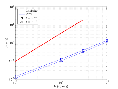
Figure 3.1. Average sampling times using Cholesky and PCG based sampling for GMRFs of size $KN$ for the simulated data $\left(K=5\right)$, with two different PCG tolerance levels $\delta$. In each case the processing time was computed as an average over 100 samples. Note that the presented PCG timings can be reduced by an additional factor in the range $[2,15]$ when a good starting value is available. The Cholesky algorithm runs out memory for $N=10^{5}$.

3.2. MCMC algorithm

In order to evaluate the true posterior of the model without any independence assumptions between parameters, we develop an algorithm for MCMC sampling. Since all priors are conjugate, we obtain closed form expressions for all full conditionals and can therefore perform Gibbs sampling. The full conditional posterior for $\mathbf{W}$ is given in (3.1) and the full conditionals for $\boldsymbol{\lambda}$ and $\boldsymbol{\alpha}$ are given by

$$\lambda_{n}|\mathbf{Y},\mathbf{W},\boldsymbol{\alpha} \sim Ga\left(\tilde{u}_{1n},\tilde{u}_{2}\right),$$ (3.4)

$$\alpha_{k}|\mathbf{Y},\mathbf{W},\boldsymbol{\lambda} \sim Ga\left(\tilde{q}_{1k},\tilde{q}_{2}\right),$$

with

$$\frac{1}{\tilde{u}_{1n}} = \frac{1}{2}\left(\mathbf{Y}_{\cdot,n}^{\prime}\mathbf{Y}_{\cdot,n}-2\mathbf{Y}_{\cdot,n}^{\prime}\mathbf{X}\mathbf{W}_{\cdot,n}+\mathbf{W}_{\cdot,n}^{\prime}\mathbf{X}^{\prime}\mathbf{X}\mathbf{W}_{\cdot,n}\right)+\frac{1}{u_{1}},$$ (3.5)

$$\tilde{u}_{2} = \frac{T}{2}+u_{2},$$

$$\frac{1}{\tilde{q}_{1k}} = \frac{1}{2}\mathbf{W}_{k,\cdot}\mathbf{D}_{w}\mathbf{W}_{k,\cdot}^{\prime}+\frac{1}{q_{1}},$$

$$\tilde{q}_{2} = \frac{N}{2}+q_{2}.$$

See Appendix A for the derivation of these and the corresponding full conditionals in the $P>0$ case.

The Gibbs algorithm returns $N_{iter}$ samples from the joint posterior of all parameters, which can be used for posterior inference about any subset of parameters. For example, given samples $\mathbf{W}^{\left(1:N_{iter}\right)}$ we can compute the marginal PPM for any $K\times 1$ contrast vector $\mathbf{c}$ as

$$P\left(\mathbf{c}^{\prime}\mathbf{W}_{\cdot,n}>\gamma|\mathbf{Y}\right)\approx\frac{1}{N_{iter}}\sum_{j=1}^{N_{iter}}I\left(\mathbf{c}^{\prime}\mathbf{W}_{\cdot,n}^{\left(j\right)}>\gamma\right),$$ (3.6)

for voxel $n$ and some activity threshold $\gamma$. Furthermore, since the MCMC posterior does not factorize over voxels, it is also meaningful and straightforward to compute the joint probability of activation for any set of voxels $E$ as

$$P\left(\mathbf{c}^{\prime}\mathbf{W}_{\cdot,E}>\gamma\boldsymbol{1}_{\left|E\right|}^{\prime}|\mathbf{Y}\right)\approx\frac{1}{N_{iter}}\sum_{j=1}^{N_{iter}}I\left(\mathbf{c}^{\prime}\mathbf{W}_{\cdot,E}^{\left(j\right)}>\gamma\boldsymbol{1}_{\left|E\right|}^{\prime}\right),$$ (3.7)

where $\boldsymbol{1}_{\left|E\right|}$ is a vector of ones of length $\left|E\right|$. Using the theory on excursion sets developed by Bolin and Lindgren, (2015), we can thereby compute the joint PPMs introduced in Yue et al., (2014) that avoid the problem of multiple hypothesis testing.

3.3. Spatial VB

Out of the two posterior independence assumptions in Penny et al., 2005b , we view the second one as the strongest, that is the assumption that the posterior for $\mathbf{W}$ factorizes over voxels. The developed MCMC algorithm relieves us from both independence assumptions, but has its limitations in terms of speed and memory. We therefore seek to develop an improved VB algorithm that maintains the efficiency gain from the first assumption of independence between the different types of parameters, but drops the second assumption and models the joint posterior of $\mathbf{W}$. We will refer to this algorithm as Spatial Variational Bayes (SVB) and to SPM’s factorized VB algorithm as Independent Variational Bayes (IVB).

The SVB posterior will be computed iteratively, just as in the IVB algorithm, for one parameter at a time given the approximate posterior of the others. If we denote $\boldsymbol{\theta}=\left\{\mathbf{W},\boldsymbol{\lambda},\boldsymbol{\alpha}\right\}$, then (Bishop,, 2006)

$$\log q\left(\theta_{j}\right)=E_{\theta_{-j}}\left[\log p\left(\mathbf{Y},\boldsymbol{\theta}\right)\right]+const,$$ (3.8)

with the expectation taken with respect to the VB posterior $q\left(\theta_{-i}\right)$. This means that for $q\left(\mathbf{W}\right)$ we get (see Appendix B)

$$\log q\left(\mathbf{w}_{r}\right) = E_{\lambda,\boldsymbol{\alpha}}\left[\log p\left(\mathbf{Y}|\mathbf{W},\boldsymbol{\lambda}\right)+\log p\left(\mathbf{W}|\boldsymbol{\alpha}\right)\right]+const$$

$$= -\frac{1}{2}\mathbf{w}_{r}^{\prime}\tilde{\mathbf{B}}^{SVB}\mathbf{w}_{r}+\mathbf{b}_{w}^{SVB\prime}\mathbf{w}_{r}+const,$$

$$\mathbf{b}_{w}^{SVB} = vec\left(diag\left(E_{\boldsymbol{\lambda}}\left[\boldsymbol{\lambda}\right]\right)\mathbf{Y}^{\prime}\mathbf{X}\right),$$

$$\tilde{\mathbf{B}}^{SVB} = \mathbf{X}^{\prime}\mathbf{X}\otimes diag\left(E_{\boldsymbol{\lambda}}\left[\boldsymbol{\lambda}\right]\right)+diag\left(E_{\boldsymbol{\alpha}}\left[\boldsymbol{\alpha}\right]\right)\otimes\mathbf{D}_{w},$$

that is, we get exactly the same expression as for the full conditionals only the values for $\boldsymbol{\lambda}$ and $\boldsymbol{\alpha}$ are replaced by their expectations with respect to their variational posteriors $q\left(\boldsymbol{\lambda}\right)$ and $q\left(\boldsymbol{\alpha}\right)$. This expression is simple because $\boldsymbol{\lambda}$ and $\boldsymbol{\alpha}$ enter linearly, which will not be the case in general. For $q\left(\boldsymbol{\alpha}\right)$ we get (note that the likelihood $p\left(\mathbf{Y}|\mathbf{W},\boldsymbol{\lambda}\right)$ does not depend on $\boldsymbol{\alpha}$)

$$\log q\left(\boldsymbol{\alpha}\right) = E_{\mathbf{W},\boldsymbol{\lambda}}\left[\log p\left(\mathbf{Y}|\mathbf{W},\boldsymbol{\lambda}\right)+\log p\left(\mathbf{W}|\boldsymbol{\alpha}\right)+\log p\left(\boldsymbol{\alpha}\right)\right]+const$$

$$= \left(\frac{N}{2}+q_{2}-1\right)\sum_{k=1}^{K}\log\alpha_{k}-\sum_{k=1}^{K}\alpha_{k}\left[\frac{1}{2}E_{\mathbf{W}}\left[\mathbf{W}_{k,\cdot}\mathbf{D}_{w}\mathbf{W}_{k,\cdot}^{\prime}\right]+\frac{1}{q_{1}}\right]+const.$$

So, just as for the full conditionals, $\alpha_{k}$ will be Gamma distributed a posteriori with parameters

$$\frac{1}{\tilde{q}_{1k}^{SVB}} = \frac{1}{2}E_{\mathbf{W}}\left[\mathbf{W}_{k,\cdot}\mathbf{D}_{w}\mathbf{W}_{k,\cdot}^{\prime}\right]+\frac{1}{q_{1}},$$ (3.11)

$$\tilde{q}_{2}^{SVB} = \frac{N}{2}+q_{2}.$$

The problem here is the expectation of the quadratic form

$$E_{\mathbf{W}}\left[\mathbf{W}_{k,\cdot}\mathbf{D}_{w}\mathbf{W}_{k,\cdot}^{\prime}\right]=E_{\mathbf{W}}\left[\mathbf{W}_{k,\cdot}\right]\mathbf{D}_{w}E_{\mathbf{W}}\left[\mathbf{W}_{k,\cdot}^{\prime}\right]+tr\left(\mathbf{D}_{w}Cov\left[\mathbf{W}_{k,\cdot},\mathbf{W}_{k,\cdot}\right]\right),$$ (3.12)

where the second term requires inversion (or at least partial inversion) of the posterior precision for $\mathbf{W}$, $\tilde{\mathbf{B}}^{SVB}$, which is computationally infeasible in the general 3D case. To avoid this, we adopt a Monte Carlo (MC) sampling based approach to compute the expectation. The PCG sampling method provides an efficient way to generate a number of ($N_{s}$) samples $\mathbf{W}^{\left(1:N_{s}\right)}$ from the VB posterior $q(\mathbf{W})$, by simply replacing $\tilde{\mathbf{B}}$ and $\mathbf{b}_{w}$ in Algorithm 2 with $\tilde{\mathbf{B}}^{SVB}$ and $\mathbf{b}_{w}^{SVB}$. These samples can be used to approximate the expectation as

$$E_{\mathbf{W}}\left[\mathbf{W}_{k,\cdot}\mathbf{D}_{w}\mathbf{W}_{k,\cdot}^{\prime}\right]\approx\frac{1}{N_{s}}\sum_{j=1}^{N_{s}}\mathbf{W}_{k,\cdot}^{\left(j\right)}\mathbf{D}_{w}\mathbf{W}_{k,\cdot}^{(j)\prime}.$$ (3.13)

Similar MC approximations will be used in the VB update equations of $\boldsymbol{\lambda}$ and for the other parameters when $P>0$, see Appendix B.

The SVB algorithm is similar to the MCMC algorithm in that the computational bottleneck will be the sampling of $\mathbf{W}$, but there are some important differences. The MCMC algorithm runs for a large number of iterations ($N_{iter}$, thousands) producing one sample from $p\left(\mathbf{W}|\mathbf{Y},\boldsymbol{\lambda},\boldsymbol{\alpha}\right)$ in each iteration. For SVB it is enough to run for a much smaller number of iterations (tens), but each iteration draws a larger number of samples ($N_{s}$, tens or hundreds) from $q\left(\mathbf{W}\right).$ When PCG based sampling is used SVB is advantageous because (i) the same pre-conditioner $\mathbf{M}$ can be used for all samples in each VB iteration (ii) the same random seeds (the same $\mathbf{z}_{1}$ and $\mathbf{z}_{2}$ in Algorithm 2) can be used across VB iterations, making the previous iteration samples very good starting values for the PCG (iii) since the samples are independent, the sampling can be fully parallelized within each iteration by running Algorithm 2 on separate cores. All these points contribute to that SVB can be run much faster than MCMC in general, with the price being the first assumption of independence between different kinds of parameters.

The MC approximation introduced in equation (3.13) adds a stochastic approximation error to the already approximate VB posterior. Figure 4.1b below quantifies the size of this error with respect to the number of samples $N_{s}$ on simulated data. Convergence results for stochastic VB methods (Kingma and Welling,, 2014; Gunawan et al.,, 2016) and for stochastic variants of the related expectation-maximization (EM) algorithm (Chan and Ledolter,, 1995; Delyon et al.,, 1999) are available in the literature. However, these results do not apply to our setting since they build on repeated sampling, while the SVB algorithm presented here only draws $\mathbf{z}_{1}$ and $\mathbf{z}_{2}$ in Algorithm 2 in the first iteration and then re-uses those same random numbers at the subsequent iterations. Re-using the random numbers speeds up SVB (typically by a factor between $2$ and $15$) since it allows us to use good PCG starting values, and the additional approximation error resulting from fixed random numbers is small in our applications. See Appendix C for more details about the convergence.

In theory, all SVB posterior statistics, such as PPMs, can be computed from the approximate posterior $q\left(\mathbf{W}\right)$ in equation (3.3). However, since it is parametrized using the precision matrix even basic marginal statistics, as variances and posterior probabilities, are not trivially obtained since this requires the inversion (or at least the Cholesky factor) of the precision matrix. We can instead use the sample variance of the samples $\mathbf{W}^{\left(1:N_{s}\right)}$ to get a fast approximation (Papandreou and Yuille,, 2011), which can be used to compute the marginal PPMs in each voxel. For contrast PPMs, we similarly use the sample covariance matrix for each voxel. While a small value of $N_{s}$ $\left(\leq 100\right)$ seems sufficient for convergence of the SVB algorithm, covariance estimates based on the same number of samples will be quite noisy (see Figure 4.2 below). A straightforward strategy to reduce the noise would be to generate additional samples from $q\left(\mathbf{W}\right)$ in a post-processing step, to further improve the covariance estimates. Such a step could be time consuming, however, and we are currently working on a different, more efficient way to compute covariances for a given sparse precision matrix.

4. Results

In this section we present results comparing the three methods (IVB, SVB and MCMC) on the same data. As MCMC is exact (in the sense of being simulation consistent with a small and controllable error), we can view this as the ground truth when evaluating the other methods. IVB is run using SPM12. The SVB algorithm is implemented as an extension to the original IVB algorithm by manipulating the original SPM12 Matlab code, while the MCMC algorithm is implemented in a separate Matlab function. The overhead time is low compared to the main computation steps for all three methods, so all timing comparisons should be considered fair. We perform the comparison on simulated data with the focus on computational efficiency as a function of data size, and on two different real data sets with the focus on the resulting posteriors and PPMs.

For any comparison to be fair, both regarding computing time and estimated posteriors, we need the different algorithms to reach the same level of convergence. In Appendix C we discuss some details on the convergence of the different methods and show that the SPM12 default setting of $4$ VB iterations is usually not sufficient. In the results below, all methods including IVB are run until convergence. In Appendix C we also provide some practical details about the implementation of respective method and about the computers used to perform the analyses.

4.1. Simulated data

We simulate synthetic data from the model, with $K=5$ and $P=1$ and pick parameter values for the voxel intercept and noise standard deviation that approximately match those of the face repetition data described below. Several different values of $\boldsymbol{\alpha}$ were used to simulate conditions with varying informativeness, see Appendix D for details. We run the algorithms on simulations of $N=10^{3}$, $10^{4}$ and $10^{5}$ voxels to get an idea how they scale and compare with the number of voxels. Figure 4.1a shows the processing time until convergence, defined as the time until the estimated posterior mean of $\boldsymbol{\alpha}$ reaches within $1\%$ of its final value, for respective algorithm. In Figure 4.1b, the accuracy of respective algorithm is evaluated. This is based on the root-mean-squared-error (RMSE) of the marginal posterior mean of activation coefficients $\mathbf{W}$ compared to the posterior mean from MCMC with $\delta=10^{-8}$.

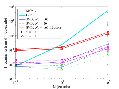
(a)

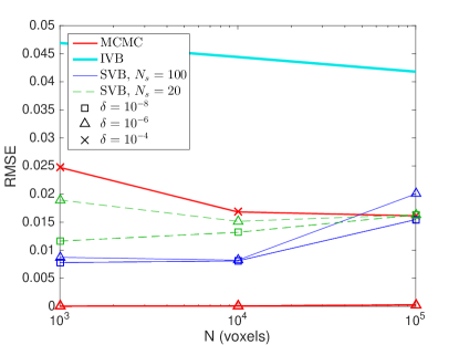
(b)

Figure 4.1. (a) Processing time as a function of the number of voxels for the different algorithms and different PCG tolerance levels $\delta$. For SVB, the number of MC samples $N_{s}$ and computing cores are also varied. The computations were made on simulated data with $K=5$ using the 3D prior. (b) RMSE of activation coefficient posterior mean for the different algorithms as compared to the MCMC posterior with $\delta=10^{-8}$, based on the first $4$ regressors.

Figure 4.1 indicates that the SVB and MCMC algorithms scale much better with the number of voxels than IVB does, and also provide a higher accuracy. Lowering the PCG tolerance $\delta$ from $10^{-8}$ to $10^{-6}$ gives some speedup while seemingly sacrificing little in accuracy. However, for $\delta=10^{-4}$ the RMSE for MCMC increases and for SVB it becomes as high as $0.25$ with very noisy convergence times (not shown), so this tolerance must not be set too high. The speedup achieved by lowering $N_{s}$ seems almost linear, but results in a lower accuracy. The speed gain in parallelizing is small due to overhead costs, but we expect greater speed-ups for larger data sets when each VB iteration requires more time, which is seen for the real data in Table 1 below. Note that the timing results in Figure 4.1 (and also in Table 1) need to be interpreted with caution since they are based on single runs of the stochastic MCMC and SVB methods, but these graphs provide insight about how the timing largely compares for the different methods and settings.

4.2. Real data

Two real task-fMRI data sets are considered, the face repetition data used in Penny et al., 2005b and data from a visual object recognition experiment from the OpenfMRI database (Poldrack et al.,, 2013), see Appendix D for more details on these data sets.

Approximate processing times for these data are shown in Table 1, both for slice-wise analysis using the 2D prior, and whole-brain analysis using the 3D prior. The IVB method scales much worse with the number of voxels and is hence slow in the 3D case, while MCMC and SVB are not necessarily slower in 3D than in 2D. For whole-brain inference with the 3D prior, SVB is generally the fastest option, especially when run in parallel.

	Face repetition				Object recognition
	2D prior	3D prior			2D prior	3D prior
IVB	4.9	190			1.9	26
MCMC	110	150			230	76
SVB	5.3	11			22	20
SVB, 4 cores	2.8	3.8			8.7	7.6

Table 1. Approximate processing times (h) for the different real data sets and algorithms using the 2D/3D prior.

We first consider the face repetition data. Figure 4.2 shows the posterior mean and standard deviation of the activation contrast, estimated using all three methods for the 2D prior. Comparing IVB to MCMC, we see bias both in the estimated IVB mean (the maximum error is 1.4 across all voxels) and standard deviation (maximum error 25%). A separate experiment with $\boldsymbol{\alpha}$ fixed to the same value for both methods showed the well-known systematic underestimation of standard deviations by IVB (roughly by 8%, results not shown). However, IVB tends to also underestimate $\boldsymbol{\alpha}$, as shown in Figure 4.6 below, leading to less shrinkage and VB errors in standard deviation that go in both directions. Comparing SVB to MCMC, we see that the estimated SVB mean is much more correct than the IVB (maximum error 0.2). However, the SVB standard deviation estimates are quite inaccurate (maximum error 26%), but this is mainly due to the noisy covariance estimates discussed in Section 3.3.

Computed marginal PPMs for various settings, thresholded at 0.9, are shown in Figure 4.3. The first row shows estimates for IVB after 4 VB iterations for the 2D prior (which is the SPM12 default), and after convergence for both the 2D and 3D prior. In the second and third row one can see the corresponding PPMs estimated using MCMC and SVB, and also the MCMC based joint PPMs which were computed using the R package excursions. The 2D joint PPM is computed based only on voxels within this slice while the 3D joint PPM is computed based on all voxels in the brain, so these maps are not directly comparable. The differences between the non-converged and converged SPM results seem rather small for this data set. Overall, the PPMs from IVB agree quite well with the PPMs from MCMC; an exception is a small cluster of activity in IVB which is lacking in the activation map from MCMC. The MCMC and SVB PPMs are hard to distinguish. Larger differences are found when comparing results based on the 2D vs. 3D prior and when comparing marginal vs. joint PPMs.

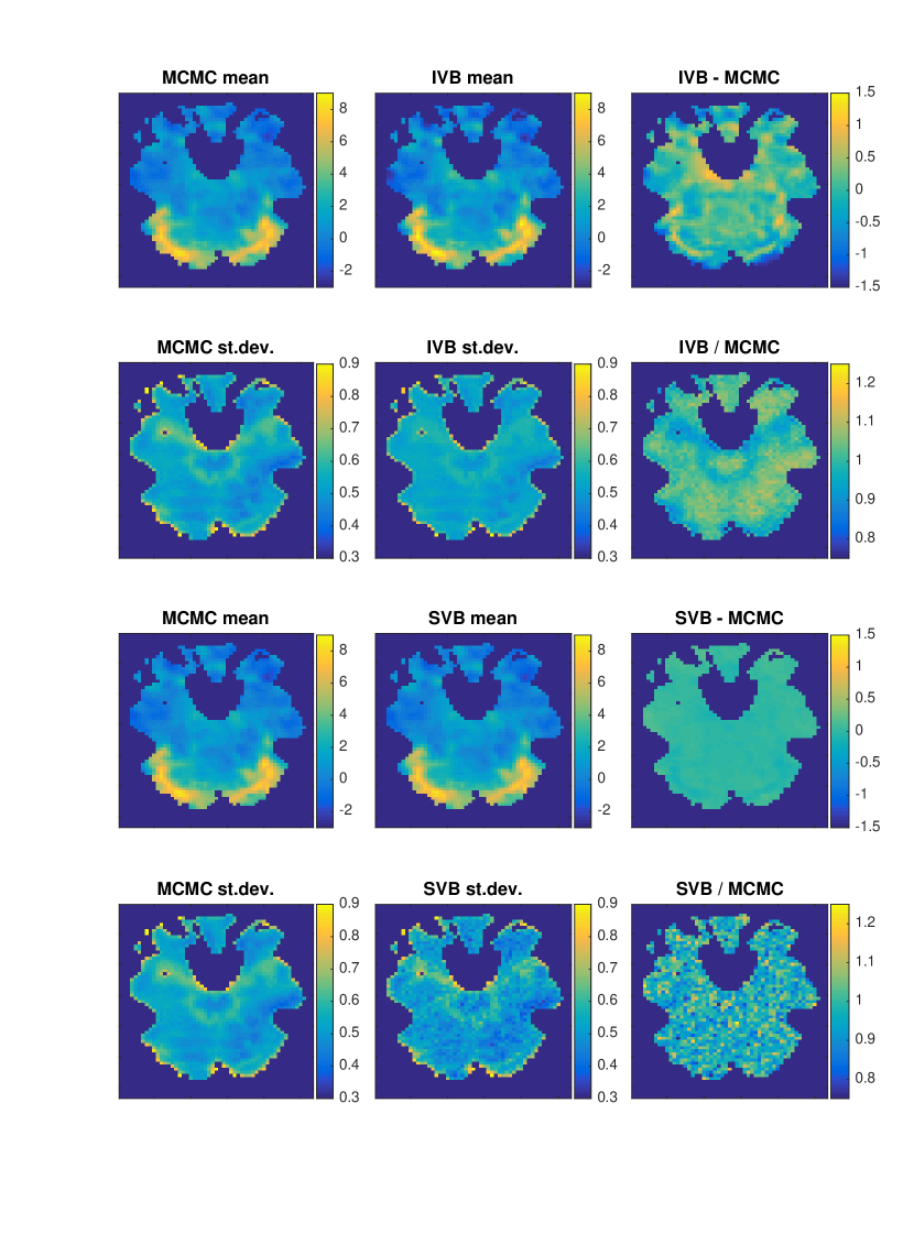
Figure 4.2. Posterior mean (top row) and standard deviation (second row) estimated using MCMC (left) and IVB (middle) for the contrast (mean effect of faces) using the 2D prior. The right column shows the differences in mean and standard deviation ratio of the estimated posteriors. Row three and four show the corresponding results for SVB.

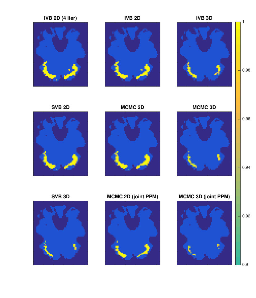
Figure 4.3. PPMs estimated for the face repetition data with different methods and 2D or 3D spatial priors. The PPMs show probabilities of the contrast (mean effect of faces) exceeding 1% of the global mean signal, thresholded at 0.9.

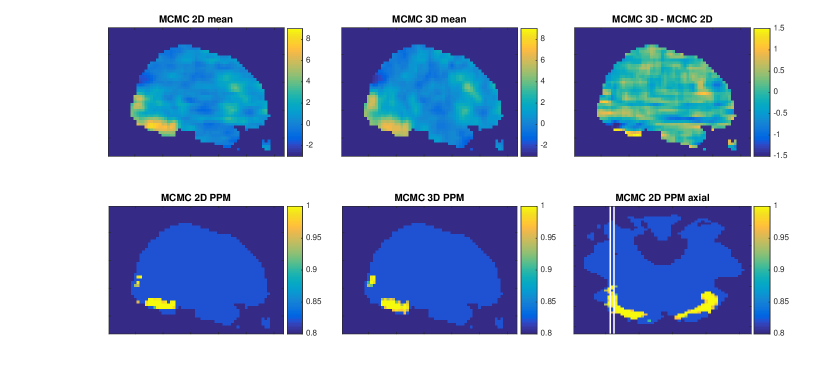
Figure 4.4. Posterior mean (top row) and marginal PPMs (bottom row) for the face repetition data for the MCMC method when using the 2D and 3D spatial priors for the sagittal slice indicated in the bottom right figure. The PPMs show probabilities of the contrast (mean effect of faces) exceeding 1% of the global mean signal, thresholded at 0.9.

The smaller activity regions from the 3D prior compared to the 2D prior is due to shrinkage towards a larger number of non-active voxels nearby in the $z$-dimension, which is depicted in Figure 4.4 that compares the posterior mean and PPM for the two priors in a sagittal slice. It is clear that the posterior mean is generally lower in the active regions when using the 3D prior, which can only be explained with the assumed dependence with non-active voxels in the $z$-dimension. For this particular slice, the effect is nevertheless strong enough for these voxels to be classified as active in the PPMs, but for other slices the higher smoothness can bring posterior probabilities below the $0.9$-threshold, for voxels classified as active when using the 2D prior. At the same time, for the 2D prior we observe discontinuous effects between slices, for example in the inferior part of the largest active blob, while the 3D prior lends strength to the voxels below, classifying them as active. It should be noted that the 2D and 3D prior lead to rather different models (the 2D prior implies a different covariance structure and has many more parameters and is therefore more flexible), so the results are not directly comparable and greatly data dependent. To decide which of these priors (or perhaps a more flexible 3D prior or parcel based method) is best is a model selection problem, which we see as important future work.

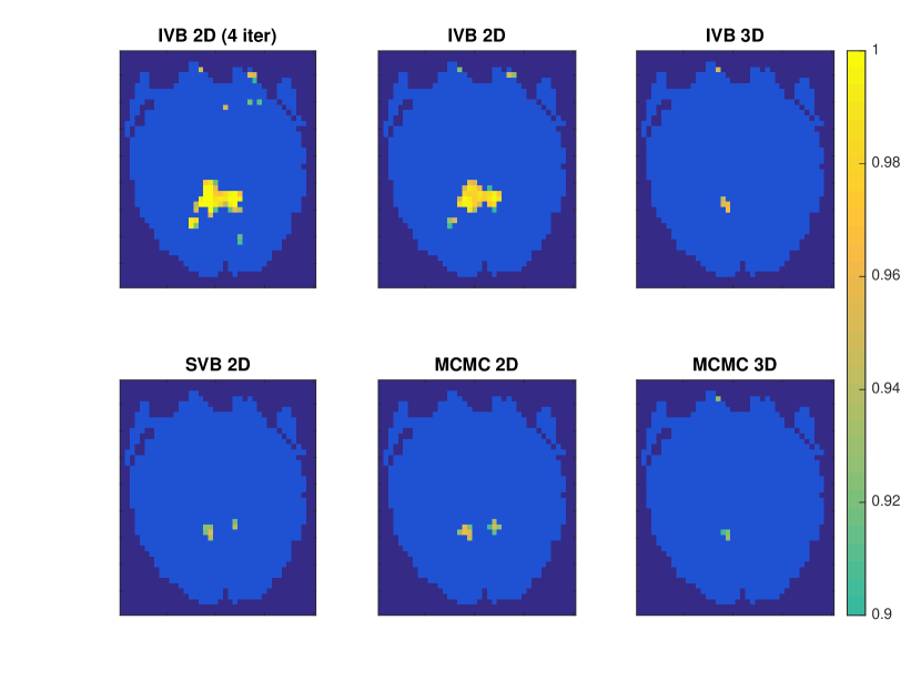
Figure 4.5. Marginal PPMs estimated for the object recognition data with different methods and 2D or 3D spatial priors. The PPMs show probabilities of the contrast (houses vs. faces) exceeding 0.5% of the global mean signal, thresholded at 0.9.

Although we observe some errors in the posterior mean and standard deviation for IVB as compared to MCMC, this error is not big enough to make much impact on the PPMs for the face repetition data set. Our second dataset, the object recognition data, shows a situation where this error can in fact be severe also for the PPMs. Figure 4.5 shows computed PPMs for one slice of the object recognition data, for some different methods and using the 2D/3D prior. It is clear that the independence assumption in IVB can lead to severely distorted activation maps, and that SVB is a much more accurate approximation for this dataset.

Much of the differences in brain maps between IVB and the other methods can be attributed to the underestimation of hyperparameters. Figure 4.6 shows the estimated posteriors of the spatial hyperparameters $\boldsymbol{\alpha}$ and $\boldsymbol{\beta}$ for the main regressors and AR coefficient for the different methods and data sets. When data are informative, as for the intercept, the VB methods generally approximate the hyperparameter posteriors well, but as data become less informative (this is clearly seen for the simulated data) the approximate posteriors from IVB underestimate both the location and dispersion of the posterior. The underestimation of posterior dispersion is a well known issue with VB quite generally (Bishop,, 2006), but the inability of IVB to correctly approximate the posterior location is unusual. The answer comes from the assumption of posterior independent voxels. Since the noise is assumed to be spatially independent, the posterior dependence between voxel activations comes solely from the spatial prior. IVB therefore pushes the $\alpha_{k}$:s to lower values in an attempt to reduce the influence of the prior. Indeed, SVB is much better at finding the correct location, but, like most VB methods, tends to underestimate the dispersion.

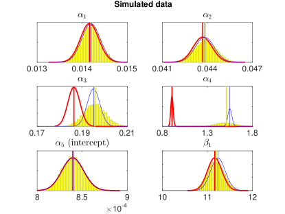
(a)

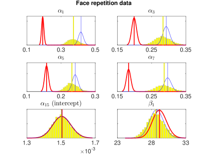
(b)

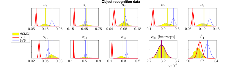
(c)

Figure 4.6. Estimated posteriors for the spatial hyperparameters for the main regressors and the first AR coefficient for the simulated (a), face repetition (b) and object recognition (c) data by MCMC (histogram), IVB (red) and SVB (blue).

5. Discussion and future work

The PCG based GMRF sampling provides a fast way to perform exact inference in high-dimensional spatial models such as the one considered here for task-fMRI. The presented results show that our methods scale better than SPM’s IVB, which is simultaneously shown to generate erroneous results for certain data.

VB approximation error

The IVB error comes from two sources. Firstly, factorized VB is known to underestimate posterior variances (Bishop,, 2006) and we have seen that fixing $\boldsymbol{\alpha}$ to the same value in both SPM’s VB and the MCMC algorithms results in underestimated $\mathbf{W}$ posterior standard deviation for IVB for the face repetition data. The same type of posterior variance underestimation can be seen for the SVB hyperparameters in Figure 4.6, a behavior that is theoretically motivated in Rue et al., (2009) (Appendix A). Secondly, we have seen that IVB tends to underestimate also the mean of $\boldsymbol{\alpha}$ for many regressors, resulting in the wrong level of smoothing/shrinkage.

The SVB method seems to approximate the exact $\mathbf{W}$ posterior well in most cases, but the underestimation of hyperparameter variance is occasionally quite large (sometimes also the mean is slightly wrong) which could motivate dropping the VB assumptions entirely and instead optimizing these parameters and perhaps using a Gaussian approximation for the uncertainty.

Computational improvements and model extensions

There is room for further improvement of the SVB method, by investigation of the sensitivity to settings like the PCG tolerance $\delta$ and the number of MC samples $N_{s}$ on a larger number of data sets. Different pre-conditioners could be used, for example the robust incomplete Cholesky (Ajiz and Jennings,, 1984), and Bolin et al., (2014) discuss other approximations of traces like the one in equation (3.12). The evaluation should be in relation to the output of interest, for example PPMs, to find the optimal balance between accuracy and processing time. In addition, a better online criterion for convergence would be beneficial. In future work we will also investigate if graphics processing units (GPUs) can be used to reduce the processing time further (Eklund et al.,, 2013, 2014).

Even though the MCMC algorithm is probably not fast enough for the everyday practitioner to run on whole-brain data sets with many conditions, it is orders of magnitude faster than what would be the case without PCG sampling, in which case it would be impractical to run at all. It fulfills an important purpose as the ground truth when evaluating approximate methods such as the VB methods in this paper, and could practically be used on sub-volumes of interest.

For the algorithms presented in this paper we have seen that the convergence rate is determined by the spatial hyperparameters for the least informative regressors. Hence, a small model change that would increase the convergence rates could be to drop the spatial prior on regressors that are very non-informative (for example motion regressors, as previously suggested by Groves et al., (2009)).

In this work, we have for brevity only considered the spatial UGL prior and focused on exact inference using this approximate model. For example, the UGL prior is stationary, isotropic and cannot separate shrinkage and smoothing. As mentioned in the introduction, many alternative, less approximate, priors have been proposed which would be interesting to adopt to the PCG sampling framework for 3D inference. Many of these would be straightforward to implement, for example the anatomically motivated tissue-type AR-priors in Penny et al., (2007), while others would require solving additional computational issues. A particularly interesting alternative would be the Matérn kernel which is a standard choice in spatial statistics. The Matérn kernel defines a Gaussian field (GF) that in general is not Markov, however, Lindgren et al., (2011) give an explicit link between GFs and GMRFs for the Matérn class such that it can be used in a sparsity exploiting manner, and they also provide a possible non-stationary Matérn model. Other parallel model improvements would be to include a spatial model also for the noise precision $\boldsymbol{\lambda}$, to add a spatial prior also for the probability of activation and to include spatial dependence in the likelihood, which is motivated by Kriegeskorte et al., (2008) who, using a phantom, demonstrate that noise from echoplanar imaging is naturally spatial.

While the voxels are normally equally sized in the $x$ and $y$ direction of each slice, this is not necessarily the case relative to the $z$ direction and one might worry that this leads to more anisotropic data that cannot be accounted for by the UGL prior. A simple solution to this is to resample the voxels to have the same size during the pre-processing, which is in fact what we did for the face repetition data, but not for the object recognition data. The same solution is possible for the second data set, but another straightforward solution would be to replace the UGL prior with a weighted graph-Laplacian (WGL) prior, that is to redefine $\mathbf{D}_{w}=\mathbf{G}_{w}^{\prime}\mathbf{C}\mathbf{G}_{w}$ instead of $\mathbf{D}_{w}=\mathbf{G}_{w}^{\prime}\mathbf{G}_{w}$ for a diagonal weight matrix $\mathbf{C}$ that can be chosen based on the Euclidian distances between neighboring voxels as in Harrison et al., 2008a . This solution would also be simply adapted to the PCG framework by just multiplying row $i$ in $\mathbf{G}_{w}$ with $\sqrt{C_{ii}}$ when using Algorithm 2. Another solution would be change the prior precision matrix in equation (2.3) from $\alpha_{k}\mathbf{G}_{w}^{\prime}\mathbf{G}_{w}$ to $\mathbf{G}_{w}^{\prime}\mathbf{C}_{k}\mathbf{G}_{w}$ with

$$\mathbf{C}_{k}=\left[\begin{array}[]{ccc}\alpha_{x,k}\mathbf{I}\\ &\alpha_{y,k}\mathbf{I}\\ &&\alpha_{z,k}\mathbf{I}\end{array}\right],$$

with $\alpha_{x,k}$, $\alpha_{y,k}$ and $\alpha_{z,k}$ being random parameters (to be inferred) that applies to neighboring pairs of voxels in the $x$, $y$ and $z$ direction respectively. Adopting such a model to the MCMC or SVB frameworks would however be difficult for computational reasons.

For inference using this or other more advanced priors than the UGL, Gibbs sampling is often not feasible. In these situations, or when the mixing of the Gibbs sampling chain is dissatisfactory, one can instead attempt to perform MCMC using Metropolis-Hastings (MH) steps or Hamiltonian Monte Carlo (HMC) (Duane et al.,, 1987; Neal,, 2011). These methods require the computation of acceptance probabilities based on the joint posterior ratio, as demonstrated for our model in Appendix A. These become computable in practice because the hyperparameters $\alpha_{k}$ can be factored out of the determinant of the prior precision matrix as in equation (A.2), but for a more advanced prior the computation of this determinant would be problematic. In a recent work, independent to ours, Teng et al., (2016) use HMC to do inference in the same model as the one in our article. They also make comparisons to SPM’s VB for the face repetition data using the 3D prior, and obtain similar results. Their reported computing times seem fast, but since they are using a much smaller model $\left(K=5\right)$ and a different implementation (C++), another number of samples, etc., their computing times cannot be directly compared to ours. Nevertheless, HMC seems like a competitive method to the proposed PCG based Gibbs sampling method for MCMC in these models. In a different, recent and independent article, Rad et al., (2016) use a similar PCG based Gibbs sampling method to ours in a similar model for other kinds of neuroscientific data. However, they use a different spatial edge-preserving Laplace prior, which would be interesting to apply also to fMRI data within this framework.

In order to be able to properly motivate any of the above mentioned model improvements, however, a model selection criterion is required. Penny et al., (2007) used the model evidence lower bound, which is a good alternative, but requires the computation of determinants of precision matrices of size $KN\times KN$, which is infeasible in the 3D case. Good approximations of such determinants would therefore be an eligible direction for future research. Model selection criteria based on cross validation or the marginal likelihood could also be explored.

Multiple comparisons

There is currently no consensus on how to control for multiple comparisons in Bayesian spatial models for fMRI data. We showed how joint PPMs based on excursion sets can be computed for the MCMC method, but the large data size is currently preventing us from computing the same for the SVB method. The joint PPMs control the family-wise error rate given the spatial model and a threshold, but a separate objective could be to instead control the false discovery rate (FDR) for which a unified framework within large-scale spatial models is provided by Sun et al., (2015). An interesting area of future research would thus be to adopt both these approaches to the 3D spatial modeling of fMRI data when using both the MCMC and SVB method.

Group analysis

Another important area of future work is to extend this single subject analysis to the group level. The simplest way to do this is to consider the posterior mean maps from the single subject analysis as spatially processed and use these as input to a voxel-wise Bayesian regression, which is basically what is done in SPM’s Bayesian second level analysis. This approach has several drawbacks, one being that mis-registration between subjects causes activation to be located in different voxels, and can therefore be missed when averaging across subjects. The classic GLM approach “handles” this by using smoothing as a pre-processing step. A more elegant, Bayesian solution is presented in Xu et al., (2009) which explicitly models population level activation centers. A second drawback is that such a procedure discards the posterior uncertainty from the subject level analyses. The most natural way to do the group level analysis would instead be using a Bayesian hierarchical model with a common group level activation working as a latent prior for each subject, and to also model the spatial hyperparameters at the group level. However, estimating such a model would intuitively be very demanding in terms of memory and speed, and an approximate idea is to instead target the mean of the subject-level activations, as in Yue et al., (2014).

5.1. In conclusion

A fast and practical MCMC scheme for exact whole-brain spatial inference in task-fMRI is suggested and implemented. Also, a non-factorizing VB method is developed and shown to give practically the same results, but in shorter time. The methods are compared to the popular factorizing VB method in SPM and shown to scale better with problem size. The comparison with the exact MCMC estimates gives evidence that SPM’s VB can produce false activity estimates in some settings.

Appendix A Derivation of full conditional posteriors for the MCMC algorithm

This section is divided into two pieces, the first handling the case when the noise in each voxel is modeled as i.i.d. over time and the second handling the case with auto-regressive temporal noise. The first part is shorter and basically contains all the concepts needed for the second part. It should be noted that adding a temporal model does not add much too the time complexity as long as $P<K$, which is normally the case. We also provide an expression for computing the joint posterior ratio.

A.1. i.i.d. noise model

The likelihood

The likelihood in (2.2) can be expressed in logs as

$$\log p\left(\mathbf{Y}|\mathbf{W},\boldsymbol{\lambda}\right) = \frac{T}{2}\sum_{n=1}^{N}\log\left(\lambda_{n}\right)$$

$$-\frac{1}{2}\sum_{n=1}^{N}\lambda_{n}\left[\mathbf{Y}_{\cdot,n}^{\prime}\mathbf{Y}_{\cdot,n}-2\mathbf{Y}_{\cdot,n}^{\prime}\mathbf{X}\mathbf{W}_{\cdot,n}+\mathbf{W}_{\cdot,n}^{\prime}\mathbf{X}^{\prime}\mathbf{X}\mathbf{W}_{\cdot,n}\right]+const,$$

where we have omitted everything that is constant with respect to the parameters. Since $\mathbf{Y}$ and $\mathbf{X}$ are data that will not change during the MCMC algorithm, quantities as $\mathbf{Y}_{\cdot,n}^{\prime}\mathbf{Y}_{\cdot,n}^{\,}$, $\mathbf{Y}_{\cdot,n}^{\prime}\mathbf{X}$ and $\mathbf{X}^{\prime}\mathbf{X}$ can be effectively pre-computed, removing the time dimension from the likelihood which leads to significant speed up. This is similar to what is done in Penny et al., 2005a .

Full conditional posterior of $\mathbf{W}$

$$\log p\left(\mathbf{W}|\mathbf{Y},\boldsymbol{\lambda},\boldsymbol{\alpha}\right) = \log p\left(\mathbf{Y}|\mathbf{W},\boldsymbol{\lambda}\right)+\log p\left(\mathbf{W}|\boldsymbol{\alpha}\right)+const$$

$$= -\frac{1}{2}\left[\sum_{n=1}^{N}\lambda_{n}\left(\mathbf{W}_{\cdot,n}^{\prime}\mathbf{X}^{\prime}\mathbf{X}\mathbf{W}_{\cdot,n}-2\mathbf{Y}_{\cdot,n}^{\prime}\mathbf{X}\mathbf{W}_{\cdot,n}\right)+\sum_{k=1}^{K}\mathbf{W}_{k,\cdot}\alpha_{k}\mathbf{D}_{w}\mathbf{W}_{k,\cdot}^{\prime}\right]+const$$

$$= -\frac{1}{2}\mathbf{w}_{r}^{\prime}\tilde{\mathbf{B}}\mathbf{w}_{r}+\mathbf{b}_{w}^{\prime}\mathbf{w}_{r}+const,$$

$$\mathbf{b}_{w} = vec\left(diag\left(\boldsymbol{\lambda}\right)\mathbf{Y}^{\prime}\mathbf{X}\right),$$

$$\tilde{\mathbf{B}} = \mathbf{X}^{\prime}\mathbf{X}\otimes diag\left(\boldsymbol{\lambda}\right)+diag\left(\boldsymbol{\alpha}\right)\otimes\mathbf{D}_{w},$$

or equivalently $\mathbf{w}_{r}|\mathbf{Y},\boldsymbol{\lambda},\boldsymbol{\alpha}\sim\mathcal{N}\left(\tilde{\mathbf{B}}^{-1}\mathbf{b}_{w},\tilde{\mathbf{B}}^{-1}\right)$, where $\mathbf{w}_{r}=vec\left(\mathbf{W}^{\prime}\right)$.

Full conditional posterior of $\boldsymbol{\lambda}$

$$\log p\left(\boldsymbol{\lambda}|\mathbf{Y},\mathbf{W},\boldsymbol{\alpha}\right) = \log p\left(\mathbf{Y}|\mathbf{W},\boldsymbol{\lambda}\right)+\log p\left(\boldsymbol{\lambda}\right)+const$$

$$= \frac{T}{2}\sum_{n=1}^{N}\log\left(\lambda_{n}\right)-\frac{1}{2}\sum_{n=1}^{N}\lambda_{n}\left[\mathbf{Y}_{\cdot,n}^{\prime}\mathbf{Y}_{\cdot,n}-2\mathbf{Y}_{\cdot,n}^{\prime}\mathbf{X}\mathbf{W}_{\cdot,n}^{\prime}+\mathbf{W}_{\cdot,n}^{\prime}\mathbf{X}^{\prime}\mathbf{X}\mathbf{W}_{\cdot,n}\right]$$

$$+\left(u_{2}-1\right)\sum_{n=1}^{N}\log\left(\lambda_{n}\right)-\sum_{n=1}^{N}\frac{\lambda_{n}}{u_{1}}+const$$

$$= \left(\tilde{u}_{2}-1\right)\sum_{n=1}^{N}\log\left(\lambda_{n}\right)-\sum_{n=1}^{N}\frac{\lambda_{n}}{\tilde{u}_{1n}}+const,$$

$$\frac{1}{\tilde{u}_{1n}} = \frac{1}{2}\left(\mathbf{Y}_{\cdot,n}^{\prime}\mathbf{Y}_{\cdot,n}-2\mathbf{Y}_{\cdot,n}^{\prime}\mathbf{X}\mathbf{W}_{\cdot,n}^{\prime}+\mathbf{W}_{\cdot,n}^{\prime}\mathbf{X}^{\prime}\mathbf{X}\mathbf{W}_{\cdot,n}\right)+\frac{1}{u_{1}},$$

$$\tilde{u}_{2} = \frac{T}{2}+u_{2},$$

so $\lambda_{n}|\mathbf{Y},\mathbf{W}\sim Ga\left(\tilde{u}_{1n},\tilde{u}_{2}\right)$ for all $n$.

Full conditional posterior of $\boldsymbol{\alpha}$

$$\log p\left(\boldsymbol{\alpha}|\mathbf{Y},\mathbf{W},\boldsymbol{\lambda}\right) = \log p\left(\mathbf{Y}|\mathbf{W},\boldsymbol{\lambda}\right)+\log p\left(\mathbf{W}|\boldsymbol{\alpha}\right)+\log p\left(\boldsymbol{\alpha}\right)+const$$

$$= \frac{N}{2}\sum_{k=1}^{K}\log\left(\alpha_{k}\right)-\frac{1}{2}\sum_{k=1}^{K}\mathbf{W}_{k,\cdot}\alpha_{k}\mathbf{D}_{w}\mathbf{W}_{k,\cdot}^{\prime}$$

$$+\left(q_{2}-1\right)\sum_{k=1}^{K}\log\left(\alpha_{k}\right)-\sum_{k=1}^{K}\frac{\alpha_{k}}{q_{1}}+const$$

$$= \left(\tilde{q}_{2}-1\right)\sum_{k=1}^{K}\log\left(\alpha_{k}\right)-\sum_{k=1}^{K}\frac{\alpha_{k}}{\tilde{q}_{1k}}+const,$$

$$\frac{1}{\tilde{q}_{1k}} = \frac{1}{2}\mathbf{W}_{k,\cdot}\mathbf{D}_{w}\mathbf{W}_{k,\cdot}^{\prime}+\frac{1}{q_{1}},$$

$$\tilde{q}_{2} = \frac{N}{2}+q_{2},$$

so $\alpha_{k}|\mathbf{W}\sim Ga\left(\tilde{q}_{1k},\tilde{q}_{2}\right)$ for all $k$.

A.2. Temporal noise model

The derivations of the full conditionals for the temporal noise model follows the same pattern as for the i.i.d. model, why we leave out some steps for brevity. Also note that the form of the posterior for the AR coefficients $\mathbf{A}$ will be very similar to that of the regression coefficients $\mathbf{W}$, and the hyperparameter $\boldsymbol{\beta}$ has the same form as $\boldsymbol{\alpha}$. The permutation matrices $\mathbf{H}_{w}$ and $\mathbf{H}_{a}$ are defined as in Penny et al., (2007) such that $vec\left(\mathbf{W}\right)=\mathbf{H}_{w}vec\left(\mathbf{W}^{\prime}\right)$ and $vec\left(\mathbf{A}\right)=\mathbf{H}_{a}vec\left(\mathbf{A}^{\prime}\right)$.

The likelihood

Using the temporal noise model, the likelihood can be expressed as

$$p\left(\mathbf{Y}|\mathbf{W},\mathbf{A},\boldsymbol{\lambda}\right)\propto\prod_{t=P+1}^{T}\prod_{n=1}^{N}\mathcal{N}\left(Y_{tn}-\mathbf{X}_{t,\cdot}\mathbf{W}_{\cdot,n};\left(\mathbf{d}_{tn}-\tilde{\mathbf{X}}_{t}\mathbf{W}_{\cdot,n}\right)^{\prime}\mathbf{A}_{\cdot,n},\lambda_{n}^{-1}\right),$$ (A.5)

where $\tilde{\mathbf{X}}_{t}$ is a $P\times K$ matrix containing the $P$ rows of the design matrix prior to time point $t$ and $\mathbf{d}_{tn}$ is $P\times 1$ and similarly contains the $P$ values of $\mathbf{Y}_{\cdot,n}$ just before $t$. Note that we condition on the first $P$ time points for simplicity. The non-constant part of the log-likelihood can be written as

$$\log p\left(\mathbf{Y}|\cdot\right) = \frac{T-P}{2}\sum_{n=1}^{N}\log\left(\lambda_{n}\right)-\frac{1}{2}\sum_{t=P+1}^{T}\sum_{n=1}^{N}\left[\left(Y_{tn}-\mathbf{X}_{t,\cdot}\mathbf{W}_{\cdot,n}\right)-\left(\mathbf{d}_{tn}-\tilde{\mathbf{X}}_{t}\mathbf{W}_{\cdot,n}\right)^{\prime}\mathbf{A}_{\cdot,n}\right]^{\prime}\lambda_{n}$$ (A.6)

$$\times\left[\left(Y_{tn}-\mathbf{X}_{t,\cdot}\mathbf{W}_{\cdot,n}\right)-\left(\mathbf{d}_{tn}-\tilde{\mathbf{X}}_{t}\mathbf{W}_{\cdot,n}\right)^{\prime}\mathbf{A}_{\cdot,n}\right]+const$$

$$= \frac{T-P}{2}\sum_{n=1}^{N}\log\left(\lambda_{n}\right)-\frac{1}{2}\sum_{n=1}^{N}\left[\left(\mathbf{Y}_{\cdot,n}-\mathbf{X}\mathbf{W}_{\cdot,n}\right)-\left(\mathbf{d}_{n}-\tilde{\mathbf{X}}\mathbf{W}_{\cdot,n}\right)^{\prime}\mathbf{A}_{\cdot,n}\right]^{\prime}\lambda_{n}$$

$$\times\left[\left(\mathbf{Y}_{\cdot,n}-\mathbf{X}\mathbf{W}_{\cdot,n}\right)-\left(\mathbf{d}_{n}-\tilde{\mathbf{X}}\mathbf{W}_{\cdot,n}\right)^{\prime}\mathbf{A}_{\cdot,n}\right]+const.$$

In the last expression the sums and indexing with respect to $t$ has been removed. Since none of the parameters depend on the time dimension, this expression can be rewritten so that sums and matrix multiplications over the time dimension can be isolated to the data $\left(\mathbf{Y},\mathbf{X},\mathbf{d},\tilde{\mathbf{X}}\right)$, so that they can be pre-computed outside the Gibbs algorithm, leading to a higher computational efficiency as in Penny et al., 2005a . Note that the size of $\mathbf{d}_{n}$ is $P\times\left(T-P\right)$ and the size of $\tilde{\mathbf{X}}$ is $P\times\left(T-P\right)\times K$. Matrix multiplications including the 3-dimensional matrix $\tilde{\mathbf{X}}$ and other tensors will be carried out over the appropriate dimension in what follows, even if this is not stated explicitly. The log-likelihood can now be rewritten as

$$\log p\left(\mathbf{Y}|\cdot\right) = \frac{T-P}{2}\sum_{n=1}^{N}\log\left(\lambda_{n}\right)$$

$$-\frac{1}{2}\sum_{n=1}^{N}\lambda_{n}\left[\mathbf{Y}_{\cdot,n}^{\prime}\mathbf{Y}_{\cdot,n}-2\mathbf{Y}_{\cdot,n}^{\prime}\mathbf{X}\mathbf{W}_{\cdot,n}+\mathbf{W}_{\cdot,n}^{\prime}\mathbf{X}^{\prime}\mathbf{X}\mathbf{W}_{\cdot,n}-2\mathbf{Y}_{\cdot,n}^{\prime}\mathbf{d}_{n}^{\prime}\mathbf{A}_{\cdot,n}\right.$$

$$+\mathbf{A}_{\cdot,n}^{\prime}\mathbf{d}_{n}\mathbf{d}_{n}^{\prime}\mathbf{A}_{\cdot,n}+\mathbf{W}_{\cdot,n}^{\prime}\mathbf{B}_{n}^{\prime}\mathbf{A}_{\cdot,n}+\mathbf{A}_{\cdot,n}^{\prime}\mathbf{B}_{n}\mathbf{W}_{\cdot,n}-\mathbf{W}_{\cdot,n}^{\prime}\left(\mathbf{R}\mathbf{A}_{\cdot,n}+\left(\mathbf{R}\mathbf{A}_{\cdot,n}\right)^{\prime}\right)\mathbf{W}_{\cdot,n}$$

$$\left.-\mathbf{A}_{\cdot,n}^{\prime}\left(\mathbf{D}_{n}\mathbf{W}_{\cdot,n}+\left(\mathbf{D}_{n}\mathbf{W}_{\cdot,n}\right)^{\prime}\right)\mathbf{A}_{\cdot,n}+\mathbf{W}_{\cdot,n}^{\prime}\left(\mathbf{A}_{\cdot,n}^{\prime}\mathbf{S}\mathbf{A}_{\cdot,n}\right)\mathbf{W}_{\cdot,n}\right]+const,$$

where

$$\mathbf{B}_{n} =\mathbf{Y}_{\cdot,n}^{\prime}\tilde{\mathbf{X}}+\mathbf{d}_{n}\mathbf{X} \text{is of size }P\times K,$$

$$\mathbf{R} =\mathbf{X}^{\prime}\tilde{\mathbf{X}} \text{is of size }K\times K\times P,$$

$$\mathbf{D}_{n} =\mathbf{d}_{n}\tilde{\mathbf{X}} \text{is of size }P\times K\times P,$$

$$\mathbf{S} =\tilde{\mathbf{X}}\tilde{\mathbf{X}} \text{is of size }P\times K\times K\times P.$$

Full conditional posterior of $\mathbf{W}$

$$\log p\left(\mathbf{W}|\mathbf{Y},\cdot\right) = -\frac{1}{2}\mathbf{w}_{r}^{\prime}\tilde{\mathbf{B}}\mathbf{w}_{r}+\mathbf{b}_{w}^{\prime}\mathbf{w}_{r}+const,$$ (A.8)

$$\mathbf{b}_{w} = vec\left(\left[\begin{array}[]{c}\vdots\\ \lambda_{n}\left(\mathbf{Y}_{\cdot,n}^{\prime}\mathbf{X}-\mathbf{A}_{\cdot,n}^{\prime}\mathbf{B}_{n}+\mathbf{A}_{\cdot,n}^{\prime}\mathbf{D}_{n}\mathbf{A}_{\cdot,n}\right)\\ \vdots\end{array}\right]_{n\in\left\{1,\ldots,N\right\}}\right),$$ (A.12)

$$\tilde{\mathbf{B}} = \mathbf{H}_{w}^{\prime}\underset{n\in\left\{1,\ldots,N\right\}}{blkdiag}\left[\lambda_{n}\left(\mathbf{X}^{\prime}\mathbf{X}-\mathbf{R}\mathbf{A}_{\cdot,n}-\left(\mathbf{R}\mathbf{A}_{\cdot,n}\right)^{\prime}+\mathbf{A}_{\cdot,n}^{\prime}\mathbf{S}\mathbf{A}_{\cdot,n}\right)\right]\mathbf{H}_{w}$$

$$+diag\left(\boldsymbol{\alpha}\right)\otimes\mathbf{D}_{w},$$

where $\underset{n\in\left\{1,\ldots,N\right\}}{blkdiag}\left[\mathbf{C}_{n}\right]$ is a $KN\times KN$ block diagonal matrix with the $K\times K$ matrix $\mathbf{C}_{n}$ as the $n$th block. So $\mathbf{w}_{r}|\mathbf{Y},\cdot\sim\mathcal{N}\left(\tilde{\mathbf{B}}^{-1}\mathbf{b}_{w},\tilde{\mathbf{B}}^{-1}\right).$

Full conditional posterior of $\mathbf{A}$

$$\log p\left(\mathbf{A}|\mathbf{Y},\cdot\right) = -\frac{1}{2}\mathbf{a}_{r}^{\prime}\tilde{\mathbf{J}}\mathbf{a}_{r}+\mathbf{b}_{a}^{\prime}\mathbf{a}_{r}+const,$$ (A.13)

$$\mathbf{b}_{a} = vec\left(\left[\begin{array}[]{c}\vdots\\ \lambda_{n}\left(\mathbf{Y}_{\cdot,n}^{\prime}\mathbf{d}_{n}^{\prime}-\mathbf{W}_{\cdot,n}^{\prime}\mathbf{B}_{n}^{\prime}+\mathbf{W}_{\cdot,n}^{\prime}\mathbf{R}\mathbf{W}_{\cdot,n}\right)\\ \vdots\end{array}\right]_{n\in\left\{1,\ldots,N\right\}}\right),$$ (A.17)

$$\tilde{\mathbf{J}} = \mathbf{H}_{a}^{\prime}\underset{n\in\left\{1,\ldots,N\right\}}{blkdiag}\left[\lambda_{n}\left(\mathbf{d}_{n}\mathbf{d}_{n}^{\prime}-\mathbf{D}_{n}\mathbf{W}_{\cdot,n}-\left(\mathbf{D}_{n}\mathbf{W}_{\cdot,n}\right)^{\prime}+\mathbf{W}_{\cdot,n}^{\prime}\mathbf{S}\mathbf{W}_{\cdot,n}\right)\right]\mathbf{H}_{a}$$

$$+diag\left(\boldsymbol{\beta}\right)\otimes\mathbf{D}_{a},$$

so $\mathbf{a}_{r}|\mathbf{Y},\cdot\sim\mathcal{N}\left(\tilde{\mathbf{J}}^{-1}\mathbf{b}_{a},\tilde{\mathbf{J}}^{-1}\right).$

Full conditional posterior of $\boldsymbol{\lambda}$

$$\log p\left(\boldsymbol{\lambda}|\mathbf{Y},\cdot\right) = \left(\tilde{u}_{2}-1\right)\sum_{n=1}^{N}\log\left(\lambda_{n}\right)-\sum_{n=1}^{N}\frac{\lambda_{n}}{\tilde{u}_{1n}}+const,$$ (A.18)

$$\frac{1}{\tilde{u}_{1n}} = \frac{1}{u_{1}}+\frac{1}{2}\left[\mathbf{Y}_{\cdot,n}^{\prime}\mathbf{Y}_{\cdot,n}-2\mathbf{Y}_{\cdot,n}^{\prime}\mathbf{X}\mathbf{W}_{\cdot,n}+\mathbf{W}_{\cdot,n}^{\prime}\mathbf{X}^{\prime}\mathbf{X}\mathbf{W}_{\cdot,n}-2\mathbf{Y}_{\cdot,n}^{\prime}\mathbf{d}_{n}^{\prime}\mathbf{A}_{\cdot,n}\right.$$

$$+\mathbf{A}_{\cdot,n}^{\prime}\mathbf{d}_{n}\mathbf{d}_{n}^{\prime}\mathbf{A}_{\cdot,n}+\mathbf{W}_{\cdot,n}^{\prime}\mathbf{B}_{n}^{\prime}\mathbf{A}_{\cdot,n}+\mathbf{A}_{\cdot,n}^{\prime}\mathbf{B}_{n}\mathbf{W}_{\cdot,n}-\mathbf{W}_{\cdot,n}^{\prime}\left(\mathbf{R}\mathbf{A}_{\cdot,n}+\left(\mathbf{R}\mathbf{A}_{\cdot,n}\right)^{\prime}\right)\mathbf{W}_{\cdot,n}$$

$$\left.-\mathbf{A}_{\cdot,n}^{\prime}\left(\mathbf{D}_{n}\mathbf{W}_{\cdot,n}+\left(\mathbf{D}_{n}\mathbf{W}_{\cdot,n}\right)^{\prime}\right)\mathbf{A}_{\cdot,n}+\mathbf{W}_{\cdot,n}^{\prime}\left(\mathbf{A}_{\cdot,n}^{\prime}\mathbf{S}\mathbf{A}_{\cdot,n}\right)\mathbf{W}_{\cdot,n}\right],$$

$$\tilde{u}_{2} = \frac{T-P}{2}+u_{2},$$

so $\lambda_{n}|\mathbf{Y},\cdot\sim Ga\left(\tilde{u}_{1n},\tilde{u}_{2}\right)$ for all $n$.

Full conditional posterior of $\boldsymbol{\alpha}$

$$\log p\left(\boldsymbol{\alpha}|\cdot\right) = \left(\tilde{q}_{2}-1\right)\sum_{k=1}^{K}\log\left(\alpha_{k}\right)-\sum_{k=1}^{K}\frac{\alpha_{k}}{\tilde{q}_{1k}}+const,$$ (A.19)

$$\frac{1}{\tilde{q}_{1k}} = \frac{1}{2}\mathbf{W}_{k,\cdot}\mathbf{D}_{w}\mathbf{W}_{k,\cdot}^{\prime}+\frac{1}{q_{1}},$$

$$\tilde{q}_{2} = \frac{N}{2}+q_{2},$$

so $\alpha_{k}|\cdot\sim Ga\left(\tilde{q}_{1k},\tilde{q}_{2}\right)$ for all $k$. This is exactly the same as for the i.i.d. case.

Full conditional posterior of $\boldsymbol{\beta}$

$$\log p\left(\boldsymbol{\beta}|\cdot\right) = \left(\tilde{r}_{2}-1\right)\sum_{p=1}^{P}\log\left(\beta_{p}\right)-\sum_{p=1}^{P}\frac{\beta_{p}}{\tilde{r}_{1p}}+const,$$ (A.20)

$$\frac{1}{\tilde{r}_{1p}} = \frac{1}{2}\mathbf{A}_{p,\cdot}\mathbf{D}_{a}\mathbf{A}_{p,\cdot}^{\prime}+\frac{1}{r_{1}},$$

$$\tilde{r}_{2} = \frac{N}{2}+r_{2},$$

so $\beta_{p}|\cdot\sim Ga\left(\tilde{r}_{1p},\tilde{r}_{2}\right)$ for all $p$.

Joint posterior ratio

The ratio of the joint posterior $p\left(\mathbf{W},\mathbf{A},\boldsymbol{\lambda},\boldsymbol{\alpha},\boldsymbol{\beta}|\mathbf{Y}\right)$ evaluated for two different sets of parameter values, $\left\{\mathbf{W},\mathbf{A},\boldsymbol{\lambda},\boldsymbol{\alpha},\boldsymbol{\beta}\right\}$ and $\left\{\mathbf{W}^{*},\mathbf{A}^{*},\boldsymbol{\lambda}^{*},\boldsymbol{\alpha}^{*},\boldsymbol{\beta}^{*}\right\}$, can be used to compare the posterior density in different points, even when the normalized joint posterior itself is not available in closed form. The ratio can be computed as the ratio of the unnormalized joint posterior $\tilde{p}\left(\mathbf{W},\mathbf{A},\boldsymbol{\lambda},\boldsymbol{\alpha},\boldsymbol{\beta}|\mathbf{Y}\right)$ defined by

$$\log\tilde{p}\left(\mathbf{W},\mathbf{A},\boldsymbol{\lambda},\boldsymbol{\alpha},\boldsymbol{\beta}|\mathbf{Y}\right) = \log\tilde{p}\left(\mathbf{Y}|\cdot\right)+\log\tilde{p}\left(\mathbf{W}|\boldsymbol{\alpha}\right)+\log\tilde{p}\left(\mathbf{A}|\boldsymbol{\beta}\right)+\log p\left(\boldsymbol{\lambda}\right)$$

$$+\log p\left(\boldsymbol{\alpha}\right)+\log p\left(\boldsymbol{\beta}\right),$$

where $\log\tilde{p}\left(\mathbf{Y}|\cdot\right)$ is defined as in equation (A.2) without the constant part,

$$\log\tilde{p}\left(\mathbf{W}|\boldsymbol{\alpha}\right) = \sum_{k=1}^{K}\left[\log\left(\left|\alpha_{k}\mathbf{D}_{w}\right|^{1/2}\right)-\frac{1}{2}\alpha_{k}\mathbf{W}_{k,\cdot}\mathbf{D}_{w}\mathbf{W}_{k,\cdot}^{\prime}\right]+const$$

$$= \sum_{k=1}^{K}\left[\frac{N}{2}\log\left(\alpha_{k}\right)-\frac{1}{2}\alpha_{k}\mathbf{W}_{k,\cdot}\mathbf{D}_{w}\mathbf{W}_{k,\cdot}^{\prime}\right]$$

and $\log\tilde{p}\left(\mathbf{A}|\boldsymbol{\beta}\right)$ is defined correspondingly.

Appendix B Derivation of Spatial VB posteriors

From equation (3.8) one sees that the SVB approximate posteriors can be derived from the full conditionals in Appendix A, since

$$\log q\left(\theta_{j}\right)=E_{\theta_{-j}}\left[\log p\left(\mathbf{Y},\boldsymbol{\theta}\right)\right]+const=E_{\theta_{-j}}\left[\log p\left(\theta_{j}|\mathbf{Y},\theta_{-j}\right)\right]+const.$$ (B.1)

The only difference is that we must take the expectation with respect to all other parameters. It turns out that the dependencies on $\boldsymbol{\lambda},\boldsymbol{\alpha}$ and $\boldsymbol{\beta}$ are always linear, so we can just replace these with their expectations $\bar{\boldsymbol{\lambda}},\bar{\boldsymbol{\alpha}}$ and $\bar{\boldsymbol{\beta}}$ under respective SVB gamma posterior. For example,

$$\bar{\alpha}_{k}=E_{\boldsymbol{\alpha}}\left[\alpha_{k}\right]=\tilde{q}_{1k}^{SVB}\cdot\tilde{q}_{2}^{SVB}.$$ (B.2)

For dependencies on $\mathbf{W}$ and $\mathbf{A}$ we use MC approximations as in (3.13) to compute the expectations, by simulating $N_{s}$ samples of $\mathbf{W}$ and $\mathbf{A}$ respectively. For brevity, we do not derive all approximate posteriors here, only $q\left(\mathbf{W}\right)$ for the temporal model as an example.

$$\log q\left(\mathbf{w}_{r}\right) = E_{\mathbf{A},\boldsymbol{\lambda},\boldsymbol{\alpha},\boldsymbol{\beta}}\left[\log p\left(\mathbf{W}|\mathbf{Y},\cdot\right)\right]+const$$

$$= -\frac{1}{2}\mathbf{w}_{r}^{\prime}E_{\mathbf{A},\boldsymbol{\lambda},\boldsymbol{\alpha},\boldsymbol{\beta}}\left[\tilde{\mathbf{B}}\right]\mathbf{w}_{r}+E_{\mathbf{A},\boldsymbol{\lambda},\boldsymbol{\alpha},\boldsymbol{\beta}}\left[\mathbf{b}_{w}\right]\mathbf{w}_{r}+const,$$

with $\tilde{\mathbf{B}}$ and $\mathbf{b}_{w}$ from equation (A.8). The expectations are computed as

$$\mathbf{b}_{w}^{SVB} = E_{\mathbf{A},\boldsymbol{\lambda},\boldsymbol{\alpha},\boldsymbol{\beta}}\left[\mathbf{b}_{w}\right]$$ (B.4)

$$= \frac{1}{N_{s}}\sum_{j=1}^{N_{s}}vec\left(\left[\begin{array}[]{c}\vdots\\ \bar{\lambda}_{n}\left(\mathbf{Y}_{\cdot,n}^{\prime}\mathbf{X}-\mathbf{A}_{\cdot,n}^{\left(j\right)\prime}\mathbf{B}_{n}+\mathbf{A}_{\cdot,n}^{\left(j\right)\prime}\mathbf{D}_{n}\mathbf{A}_{\cdot,n}^{\left(j\right)}\right)\\ \vdots\end{array}\right]_{n\in\left\{1,\ldots,N\right\}}\right)$$ (B.8)

$$\tilde{\mathbf{B}}^{SVB} = E_{\mathbf{A},\boldsymbol{\lambda},\boldsymbol{\alpha},\boldsymbol{\beta}}\left[\tilde{\mathbf{B}}\right]$$ (B.9)

$$= \frac{1}{N_{s}}\sum_{j=1}^{N_{s}}\mathbf{H}_{w}^{\prime}\underset{n\in\left\{1,\ldots,N\right\}}{blkdiag}\left[\bar{\lambda}_{n}\left(\mathbf{X}^{\prime}\mathbf{X}-\mathbf{R}\mathbf{A}_{\cdot,n}^{\left(j\right)}-\left(\mathbf{R}\mathbf{A}_{\cdot,n}^{\left(j\right)}\right)^{\prime}+\mathbf{A}_{\cdot,n}^{\left(j\right)\prime}\mathbf{S}\mathbf{A}_{\cdot,n}^{\left(j\right)}\right)\right]\mathbf{H}_{w}$$

$$+diag\left(\bar{\boldsymbol{\alpha}}\right)\otimes\mathbf{D}_{w}.$$

So $q\left(\mathbf{W}\right)\sim\mathcal{N}\left(\left(\tilde{\mathbf{B}}^{SVB}\right)^{-1}\mathbf{b}_{w}^{SVB},\left(\tilde{\mathbf{B}}^{SVB}\right)^{-1}\right).$

Appendix C convergence and implementation details

Our experience from running the MCMC and VB methods is that the convergence of the algorithms is largely governed by that of the spatial hyperparameters $\boldsymbol{\alpha}$ and $\boldsymbol{\beta}$. Figure C.1a shows the relative error by iteration number for the hyperparameters for IVB, for the presented slice of the face repetition data. The relative error is here defined as compared to the final value after a long run (200 iterations) and if $\bar{\alpha}_{k}^{\left[j\right]}$ denotes the value of $\bar{\alpha}_{k}$ after $j$ iterations, then the relative error $\epsilon_{k}=\left|\nicefrac{{\bar{\alpha}_{k}^{\left[j\right]}}}{{\bar{\alpha}_{k}^{\left[200\right]}}}-1\right|$ for the $k$th parameter. We see that $\bar{\alpha}_{k}$ converges the fastest for the intercept, a bit slower for regressors connected to the HRF and its temporal derivative and for the AR coefficients, and the slowest for the head motion nuisance regressors.

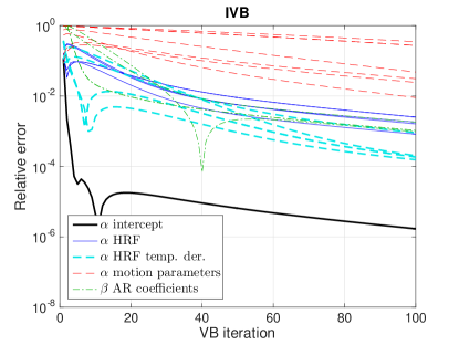
(a)

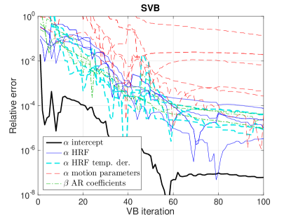
(b)

Figure C.1. Spatial hyperparameter relative errors by VB iteration number, relative to the value after 200 iterations, for the face repetition data. The errors for IVB are shown in (a), while the errors for SVB are shown in (b). The regression coefficient hyperparameters $\boldsymbol{\alpha}$ are divided by regressor type and $\boldsymbol{\beta}$ are the hyperparameters for the AR coefficients.

To understand why the parameters differ in convergence speed one has to consider how the VB algorithm works, updating the approximate posterior for $\mathbf{W}$ given $\boldsymbol{\alpha}$ and vice versa. Since $\boldsymbol{\alpha}$ controls the smoothness and shrinkage of $\mathbf{W}$, there will be much dependence between the estimated posteriors of these two parameters, leading to slower convergence. In general, the more informative the data are the faster is seemingly the convergence. For example, for $k$ corresponding to the intercept in every voxel, $\mathbf{W}_{k,\cdot}$ is quite well defined from the data, so it will depend relatively little on $\alpha_{k}$. Given the smoothness of $\mathbf{W}_{k,\cdot}$, $\alpha_{k}$ is also well determined, so convergence will be quick. On the other hand, for $k$ corresponding to head motion, $\mathbf{W}_{k,\cdot}$ will be non-significant in most voxels, giving more dependence with $\boldsymbol{\alpha}$ and slower convergence.

It takes almost 50 iterations for all the HRF regressor $\alpha_{k}$:s (which are the most interesting ones for PPMs) to reach a relative error smaller than $1\%$ for the IVB algorithm. This is interesting, since the SPM12 default setting is to use 4 VB iterations and the other available stopping criterion, based on the model evidence lower bound, results in 8 iterations. Even though this might seem as too few, the effect of this on the PPMs is not necessarily so large (see Figure 4.3 and 4.5), so keeping the number of iterations low might well be a reasonable strategy in order to reduce the processing time.

The SVB convergence plot would look similar to that of IVB, if implemented directly as it is presented above. However, we added some ad hoc steps to the SVB algorithm to speed up convergence. In contrast to IVB, the posterior update step for $q\left(\mathbf{W}\right)$ only depends on the other parameters (in particular on $\boldsymbol{\alpha}$) and the data, but not on the previous iteration value of $q\left(\mathbf{W}\right)$. Therefore, if there is some faster way to approach the optimal value of $\bar{\boldsymbol{\alpha}}$, than the SVB update equation for $q\left(\boldsymbol{\alpha}\right)$, that speedup will transfer to $q\left(\mathbf{W}\right)$ as well. In the SVB implementation we use three ad hoc tricks to speed up convergence, which we have noticed work well in practice:

1. In every other VB iteration, instead of accepting the $\tilde{q}_{1k}^{SVB\left[j\right]}$ (and hence $\bar{\alpha}_{k}^{\left[j\right]}=\tilde{q}_{1k}^{SVB\left[j\right]}\cdot\tilde{q}_{2}^{SVB}$) from the VB update equation, we fit a quadratic function to the values of the last three iterations, $\bar{\alpha}_{k}^{\left[j-2\right]}$, $\bar{\alpha}_{k}^{\left[j-1\right]}$ and $\bar{\alpha}_{k}^{\left[j\right]}$, as a function of the iteration number $j$. If the vertex of the quadratic function occurs after $j$, we take the value of the function at the vertex as a prediction of what $\bar{\alpha}_{k}$ will converge to. Otherwise, we assume that we are far from the final value and set the prediction to $\bar{\alpha}_{k}^{\left[j-1\right]}+20\left(\bar{\alpha}_{k}^{\left[j\right]}-\bar{\alpha}_{k}^{\left[j-1\right]}\right).$ We set $\bar{\alpha}_{k}^{\left[j\right]}$ to the predicted value but only allow changes in alpha up to a factor $5$ from the value proposed by the VB update equation. This methodology will make the SVB algorithm behave less stable, but allow for larger steps when $\bar{\alpha}_{k}$ is far from the final value which leads to faster convergence, especially when data are not so informative.

2. We use the prior mean as starting values for all parameters, which is a little different from what SPM’s IVB does, but leads to faster convergence for the SVB algorithm.

3. In the first $10$ iterations of the SVB algorithm we use $N_{s}=5$, which will make these iterations quicker, but not as exact.

The effect of using these tricks can be seen in Figure C.1b, showing faster convergence for the hyperparameters using SVB as compared to IVB.

Different random seeds in the MC approximation (equation (3.13)) make the SVB algorithm converge to slightly different posteriors. We reran SVB several times with $N_{s}=100$ and different seeds, and found very small differences in the results for the simulated data, but for some real data sets we found that the differences could be slightly larger. SVB appears to sometimes get stuck in local modes of the model evidence lower bound that is implicitly optimized by the VB algorithm. The resulting SVB posteriors for all of these modes were however always closer to the exact MCMC posterior than the IVB posterior was. Since the model evidence lower bound is computationally intractable, we instead compared the different modes using the joint posterior ratio in equation (A.2) evaluated in the SVB posterior mean to decide which results to present for these problematic data sets. The same multimodal issues were not observed when rerunning MCMC with different seeds or IVB with different starting values.

The MCMC Gibbs algorithm suffers from the same problem with the dependence between $\mathbf{W}$ and $\boldsymbol{\alpha}$, slowing down convergence. Inspecting trace plots and the estimated inefficiency factor $IF=1+2\sum_{j=1}^{\infty}\rho_{j}$, where $\rho_{j}$ is the autocorrelation function of the MCMC chain, for different data sets shows that the convergence for the parameters $\mathbf{W}$, $\mathbf{A}$ and $\boldsymbol{\lambda}$ is generally excellent. For example, the maximum IF was less than $1.5$ across all regression coefficients $\mathbf{W}$ for both the real data sets when using the 3D prior, except for the head motion nuisance regressors. With $20000$ post-burnin iterations and thinning factor $5$, this means that we have at least $4000/1.5\approx 2700$ effective samples to base the PPMs on, and Monte Carlo standard deviations less than $\sqrt{\frac{0.9\cdot 0.1}{2700}}\approx 0.0058$ for posterior probabilities larger that $90\%$. We also looked at posterior mean maps and PPMs for the main contrast for the different data sets and compared to the same maps computed based only on the first $5000$, $10000$ and $15000$ samples respectively, and saw small differences in general, much smaller than for example when comparing to the VB maps. The spatial hyperparameters $\boldsymbol{\alpha}$ and $\boldsymbol{\beta}$ can however mix poorly, especially when the data are non-informative. It would be tempting to improve the mixing using a collapsed Gibbs sampling step for $\boldsymbol{\alpha}$ (and $\boldsymbol{\beta}$), but this would require the computation of the precision matrix determinant $\left|\tilde{\mathbf{B}}\right|,$ which would be too time consuming in general. For the main parameters of interest, the $\alpha_{k}$:s belonging to the HRF regressors, and also for the hyperparameters belonging to the intercept and to the first AR coefficients, the convergence rates are acceptable in general. A $1000$ iteration burnin is usually sufficient to reach stationarity for these hyperparameters.

In the timing comparisons in the results section, all methods were run for a long time (200 iterations for IVB, 50 iterations for SVB and 10000 (simulated data) / 20000 (real data) iterations with thinning factor 5 after 1000 burnin samples for MCMC (an exception was MCMC in 3D for the face repetition data, which required 3500 burnin samples)) and we compute the time until the estimated posterior mean of $\alpha_{k}$ reaches within $1\%$ of its final values for respective algorithm. For VB, this is the same as based on the relative error defined above, and for MCMC this is based on the relative error of the cumulative mean of MCMC samples. For the simulated data, this is based on all $\alpha_{k}$, but for the real data we only consider the $\alpha_{k}$ corresponding to the intercept and HRF regressors. This is because the convergence is sometimes extremely slow for $\alpha_{k}$:s corresponding to the head motion and HRF temporal derivative regressors, while these have negligible effects on the results. For the real data, we use $\delta=10^{-8}$ and $N_{s}=100$ throughout.

The simulated data were analyzed on a computing cluster, using two 8-core (16 threads) Intel Xeon E5-2660 processors at 2.2GHz. The real data were mainly analyzed on the same cluster, but some demanding runs were carried out on a faster workstation with a 4-core (8 threads) Intel Xeon E5-1620 processor at 3.5GHz. The workstation ran 46% faster for a large SVB estimation test and therefore the timings using this computer were multiplied with a factor $1/0.54$ in this report, hence the word “approximate” in Table 1. The operating system was Linux in both cases.

Appendix D Simulated and real data details

The synthetic data are simulated from the model in Section 2, with $K=5$ and $P=1$ and parameter values that are similar to those of the pre-processed face repetition data. The design matrix is set to have the first 4 columns equal to the standard canonical HRF regressors from the paradigm in the face repetition data (so $T=351$) and the fifth column corresponds to the intercept. The intercept of each voxel is sampled i.i.d. from a $\mathcal{N}\left(900,130^{2}\right)$-distribution. $\lambda_{n}^{-1}=100$ for each voxel and the other hyperparameters are set as $\alpha_{1}=10^{-4},\alpha_{2}=5\cdot 10^{-4},\alpha_{3}=2\cdot 10^{-3},\alpha_{4}=10^{-2},\beta_{1}=10$, which generate reasonable values of for the $\mathbf{W}$ and $\mathbf{A}$, with varying levels of informativeness. $\mathbf{W}_{k,\cdot}$ (and similarly $\mathbf{A}$) are sampled independently for $k\in\left\{1,2,3,4\right\}$ from the UGL prior using PCG with $\mathbf{B}_{data}=\mathbf{0}$ and $\mathbf{w}_{r}^{start}=\mathbf{0}$. Even though the UGL prior is improper this works well and generates samples with mean close to zero. Conditioned on the parameters the simulation of fMRI-data $\mathbf{Y}$ is straightforward using the model. The data are simulated in a big rectangular block of size $53\times 63\times 46$ and we follow the SPM default to scale down the value in each voxel to get mean 100. We then use centered masks of size $10\times 10\times 10$, $25\times 20\times 20$ and $50\times 50\times 40$ to obtain data of size $N=10^{3}$, $10^{4}$ and $10^{5}$ that we test the methods on.

The real data from the face repetition experiment (Henson et al.,, 2002), previously used in Penny et al., 2005b and available at SPM’s homepage
(http://www.fil.ion.ucl.ac.uk/spm/data/face_rep/), was pre-processed using the same steps as in Penny et al., 2005b using SPM12. After masking away voxels outside the brain, this results in a data set with $N=57535$ voxels of size $3\times 3\times 3$ mm and $T=351$ volumes. Using the same design matrix based on the canonical HRF and its temporal derivative, 6 head motion parameters and an intercept, we have $K=15$. The contrast considered is the main effect of faces which is the mean across the four regressors corresponding to the HRF of each condition. $P=3$ AR parameters are used for all estimations on real data. The presented PPMs for this data set show axial slice 12, which is approximately the same region shown in Penny et al., 2005b .

The real data from the visual object recognition experiment (Haxby et al.,, 2001; Hanson et al.,, 2004; O’Toole et al.,, 2005) was obtained from the OpenfMRI database
(http://openfmri.org/). Its accession number is ds000105 and we consider only subject001, run001. The data was pre-processed using the same SPM pipeline as for the face repetition data, except no slice time correction was performed (since the slice order information is missing) neither was it normalized to a standard brain. This data set has $N=31241$ voxels of size $3.125\times 3.125\times 4$ mm and $T=121$. There are 8 conditions and using the same structure for the design matrix as for the face experiment data, we have $K=23$. The contrast considered is the difference between seeing houses and faces ($c_{1}=0.5$ and $c_{15}=-0.5$). The axial slice presented in the results is number 30.

References

- SPM, (2002) (2002). SPM. Wellcome Department of Imaging Neuroscience, Available at http://www.fil.ion.ucl.ac.uk/spm/software.
- Ajiz and Jennings, (1984) Ajiz, M. A. and Jennings, A. (1984). A robust incomplete Cholesky-conjugate gradient algorithm. Int. J. Numer. Meth. Engng., 20:949–966.
- Amestoy et al., (1996) Amestoy, P. R., Davis, T. A., and Duff, I. S. (1996). An Approximate Minimum Degree Ordering Algorithm. SIAM. J. Matrix Anal. & Appl., 17(4):886–905.
- Barrett et al., (1994) Barrett, R., Berry, M. W., Chan, T. F., Demmel, J., Donato, J., Dongarra, J., Eijkhout, V., Pozo, R., Romine, C., and Van der Vorst, H. (1994). Templates for the solution of linear systems: building blocks for iterative methods, volume 43. Siam.
- Besag, (1974) Besag, J. (1974). Spatial Interaction and the Statistical Analysis of Lattice Systems. Journal of the Royal Statistical Society. Series B (Methodological), 36(2):192–236.
- Bishop, (2006) Bishop, C. M. (2006). Pattern Recognition and Machine Learning. Springer.
- Bolin and Lindgren, (2015) Bolin, D. and Lindgren, F. (2015). Excursion and contour uncertainty regions for latent Gaussian models. Journal of the Royal Statistical Society: Series B (Statistical Methodology), 77(1):85–106.
- Bolin et al., (2014) Bolin, D., Wallin, J., and Lindgren, F. (2014). Multivariate latent Gaussian random field mixture models. Preprint Dept. Math. Sci., Chalmers University of Technology and Göteborg University 2014:1.
- Chaari et al., (2013) Chaari, L., Vincent, T., Forbes, F., Dojat, M., and Ciuciu, P. (2013). Fast Joint Detection-Estimation of Evoked Brain Activity in Event-Related fMRI Using a Variational Approach Lotfi. IEEE Transactions on Medical Imaging, 32(5):821–837.
- Chan and Ledolter, (1995) Chan, K. S. and Ledolter, J. (1995). Monte Carlo EM Estimation for Time Series Models Involving Counts. Journal of the American Statistical association, 90(429):242–252.
- Delyon et al., (1999) Delyon, B., Lavielle, M., and Moulines, E. (1999). Convergence of a stochastic approximation version of the EM algorithm. Annals of Statistics, 27(1):94–128.
- Duane et al., (1987) Duane, S., Kennedy, A. D., Pendleton, B. J., and Roweth, D. (1987). Hybrid Monte Carlo. Physics letters B, 195(2):216–222.
- Eklund et al., (2013) Eklund, A., Dufort, P., Forsberg, D., and LaConte, S. (2013). Medical image processing on the GPU - Past, present and future. Medical Image Analysis, 17:1073–1094.
- Eklund et al., (2014) Eklund, A., Dufort, P., Villani, M., and LaConte, S. (2014). BROCCOLI: Software for fast fMRI analysis on many-core CPUs and GPUs. Frontiers in Neuroinformatics, 8:24.
- Eklund et al., (2016) Eklund, A., Nichols, T. E., and Knutsson, H. (2016). Cluster failure: why fMRI inferences for spatial extent have inflated false positive rates. Proceedings of the National Academy of Sciences, 113(28):7900–7905.
- Friston et al., (1995) Friston, K. J., Holmes, a. P., Worsley, K. J., Poline, J.-P., Frith, C. D., and Frackowiak, R. S. J. (1995). Statistical parametric maps in functional imaging: A general linear approach. Human Brain Mapping, 2(4):189–210.
- Friston and Penny, (2003) Friston, K. J. and Penny, W. (2003). Posterior probability maps and SPMs. NeuroImage, 19(3):1240–1249.
- Groves et al., (2009) Groves, A. R., Chappell, M. A., and Woolrich, M. W. (2009). Combined spatial and non-spatial prior for inference on MRI time-series. NeuroImage, 45(3):795–809.
- Gunawan et al., (2016) Gunawan, D., Tran, M., and Kohn, R. (2016). Fast Inference for Intractable Likelihood Problems using Variational Bayes. preprint: http://hdl.handle.net/2123/14594.
- Hanson et al., (2004) Hanson, S. J., Matsuka, T., and Haxby, J. V. (2004). Combinatorial codes in ventral temporal lobe for object recognition: Haxby (2001) revisited: is there a "face" area? NeuroImage, 23(1):156–166.
- Harrison and Green, (2010) Harrison, L. M. and Green, G. G. R. (2010). A Bayesian spatiotemporal model for very large data sets. NeuroImage, 50(3):1126–1141.
- (22) Harrison, L. M., Penny, W., Daunizeau, J., and Friston, K. J. (2008a). Diffusion-based spatial priors for functional magnetic resonance images. NeuroImage, 41(2):408–423.
- (23) Harrison, L. M., Penny, W., Flandin, G., Ruff, C. C., Weiskopf, N., and Friston, K. J. (2008b). Graph-partitioned spatial priors for functional magnetic resonance images. NeuroImage, 43(4):694–707.
- Haxby et al., (2001) Haxby, J. V., Gobbini, M. I., Furey, M. L., Ishai, A., Schouten, J. L., and Pietrini, P. (2001). Distributed and Overlapping Representations of Faces and Objects in Ventral Temporal Cortex. Science, 293(5539):2425–2430.
- Henson et al., (2002) Henson, R., Shallice, T., Gorno-Tempini, M. L., and Dolan, R. (2002). Face repetition effects in implicit and explicit memory tests as measured by fMRI. Cerebral Cortex, 12:178–186.
- Kingma and Welling, (2014) Kingma, D. P. and Welling, M. (2014). Auto-Encoding Variational Bayes. arXiv:1312.6114v10.
- Kriegeskorte et al., (2008) Kriegeskorte, N., Bodurka, J., and Bandettini, P. (2008). Artifactual time-course correlations in echo-planar fMRI with implications for studies of brain function. International Journal of Imaging Systems and Technology, 18(5-6):345–349.
- Lindgren et al., (2011) Lindgren, F., Rue, H., and Lindström, J. (2011). An explicit link between Gaussian fields and Gaussian Markov random fields: The SPDE approach. Journal of the Royal Statistical Society Series B, 73(4):423–498.
- Manteuffel, (1980) Manteuffel, T. a. (1980). An incomplete factorization technique for positive definite linear systems. Mathematics of Computation, 34(150):473–473.
- Musgrove et al., (2016) Musgrove, D. R., Hughes, J., and Eberly, L. E. (2016). Fast, fully Bayesian spatiotemporal inference for fMRI data. Biostatistics, 17(2):291–303.
- Neal, (2011) Neal, R. M. (2011). MCMC using Hamiltonian dynamics. Handbook of Markov Chain Monte Carlo, pages 113–162.
- O’Toole et al., (2005) O’Toole, A. J., Jiang, F., Abdi, H., and Haxby, J. V. (2005). Partially Distributed Representations of Objects and Faces in Ventral Temporal Cortex. Journal of Cognitive Neuroscience, 17(4):580–590.