Bending and Gaussian rigidities of confined soft spheres from second-order virial series

Abstract

We use virial series to study the equilibrium properties of confined soft-spheres fluids interacting through the inverse-power potentials. The confinement is induced by hard walls with planar, spherical and cylindrical shapes. We evaluate analytically the coefficients of order two in density of the wall-fluid surface tension $\gamma$ and analyze the curvature contributions to the free energy. Emphasis is in bending and Gaussian rigidities, which are found analytically at order two in density. Their contribution to $\gamma(R)$ and the accuracy of different truncation procedures to the low curvature expansion are discussed. Finally, several universal relations that apply to low-density fluids are analyzed.

I Introduction

Inhomogeneous fluid systems with interfaces have been studied for a long time and are ubiquitous in nature. Characteristic examples of such systems are the two phase coexistence with vapor-liquid interface and the confined system with fluid-wall interface. In the second case the interface is induced by an external potential that yields spatial regions forbidden for the fluid. From a thermodynamic perspective the correspondence between the free-energy of the system and the shape of its interface is a relevant topic both for basic and applied investigation.

Confined fluids enable us to study in a simple manner the dependence of the interface free energy with the interface shape by simply changing the shape of the vessel. In particular, smooth interfaces are appropriate to analyze the deviation from the well-known planar limit where the theoretical framework is established. Even for low-density confined fluids the first principles theories based in virial series approach are still under development. Seminal work of Bellemans dates from the 1960’s (Bellemans, 1962a, b, 1963) and later developments of Rowlinson and McQuarrie (Rowlinson, 1985; McQuarrie and Rowlinson, 1987) were done in the 1980’s. Recently, new exact results based on virial series were obtained for confined hard spheres (HS),(Yang et al., 2013; Urrutia, 2014a, b) square well, and even Lennard-Jones, systems.(Urrutia and Paganini, 2016) This work aims to contribute in this direction by studying the physical properties of pure repulsive soft-spheres system confined by curved walls.

The soft-sphere particles interact through a tuneable softness core (without an attractive well) produced by the inverse-power law potential (IPL). This model has interesting scaling properties(Hoover et al., 1970; Rosenfeld, 1983; Kohl and Schmiedeberg, 2014) and constitutes an important reference to study more complex systems.(Hansen, 1970; Kambayashi and Hiwatari, 1994; Hummel et al., 2015) Several studies focused on elucidating the relation between core-softness and thermodynamic properties.(Lange et al., 2009; Shi et al., 2011; Wheatley, 2013; Zhou and Solana, 2013) Basic research about bulk transport and virial coefficients was started by Rainwater and others,(Rainwater, 1978, 1979; Dixon and Hutchinson, 1979; Kayser, 1980; Rainwater, 1981, 1984) and continues up to present.(Wheatley, 2005; Tan et al., 2011; Barlow et al., 2012; Wheatley, 2013) Analytic equations of state of the soft-sphere fluid were found using as input the known bulk virial coefficients using resummation, by adapting the Carnahan Starling equation of state for HS to soft-spheres and utilizing Padé approximants.(Maeso and Solana, 1993; Tan et al., 2011; Barlow et al., 2012) Aspects of recent research interest in the soft-sphere system are the scaling law invariance of its properties,(Pieprzyk et al., 2014; Hummel et al., 2015) the enhancement of effective attraction between colloids produced by the soft repulsion in colloid+depletants system,(Rovigatti et al., 2015) the equilibrium and nonequilibrium dynamics of particles,(Ding and Mittal, 2015) and the analysis of the sound velocity near the fluid-solid phase transition.(Khrapak, 2016)

We will study the dependence on curvature of equilibrium thermodynamic properties of the fluid confined by curved walls based on its inhomogeneous second virial coefficient. For simplicity only constant-curvature surfaces, i.e., planar, spherical, and cylindrical, are considered. The expansion of the wall-fluid surface tension on the surface curvature follows the Helfrichs expression.(Helfrich, 1973) Applied to the sphere and cylinder symmetry the expansion of $\gamma(R)$ gives

$$\gamma_{\textrm{s}}(R) = \gamma-\frac{2\gamma\delta}{R}+\frac{2k+\bar{k}}{R^{2}}+\frac{\mathscr{C}}{R^{3}}+\ldots\>,$$ (1)

$$\gamma_{\textrm{c}}(R) = \gamma-\frac{\gamma\delta}{R}+\frac{k}{2R^{2}}+\ldots\>,$$ (2)

where dots represent higher-order terms in $R^{-1}$. Here, $\gamma$ is the wall-fluid surface tension for a planar surface and $\delta$ is the (radius-independent) Tolman length, which is related with the total curvature. Next term beyond $\gamma\delta$ includes the bending rigidity $k$ (associated with the square of the total curvature) and the Gaussian rigidity $\bar{k}$ (associated with Gaussian curvature). In the present work we will analyze Eqs. (1,2) using virial series expansion.

In the following Sec. II it is given a brief review of the statistical mechanics virial series approach to inhomogeneous fluids. The second-order cluster integral is analytically evaluated for the confined soft-sphere system interacting through IPL in Sec. III. There, the functional dependence on the hardness parameter $\nu$, the temperature, and the radius is shown. Surface tension is studied at low density as a function of $\nu$ and $R$ in Sec. IV. In Sec. V the bending and Gaussian curvature rigidity constants are extracted and studied as a function of $\nu$. It is found that for $\nu=6$ there exists a logarithmic term in the surface free-energy that corresponds to curvature rigidities and that is absent for $\nu>6$. Several recently found universal relations that apply to any fluid are here verified for soft spheres. Besides, our exact results and some of these universal relations are used to test the degree of accuracy of morphometric approach at low density. Finally, a summary is given in Sec. VI.

II Statistical Thermodynamic background

The following short summary about virial series for confined systems attempts to give a closed-form of the general theory and contains a collection of ideas and formulae taken from Refs. (Rowlinson, 1985; Urrutia, 2011; Urrutia and Castelletti, 2012; Yang et al., 2013). The virial series of the free energy here developed will be used in Secs. III to V to study the confined IPL system up to order two in the activity (the lowest nontrivial order).

We consider an inhomogeneous fluid at a given temperature $T$ and chemical potential $\mu$ under the action of an external potential. The grand canonical ensemble partition function (GCE) of this system is

$$\Xi=1+\sum_{n=1}\lambda^{n}Q_{n}\>,$$ (3)

where $\lambda=\exp(\beta\mu)$ and $\beta=1/k_{\textrm{B}}T$ is the inverse temperature ($k_{\textrm{B}}$ is the Boltzmann’s constant). In Eq. (3) $Q_{n}$ is the canonical ensemble partition function

$$Q_{n} = \Lambda^{dn}Z_{n}/n!\>,$$ (4)

$$Z_{n} = \int g_{n}\left(\mathbf{x}\right)\exp\left(-\beta\phi_{(n)}\right)d\mathbf{x}\>,$$ (5)

where $\Lambda$ is the de Broglie thermal wavelength and $d$ is dimension. $Z_{n}$ is the configuration integral, $\phi_{(n)}$ is the interaction potential between particles, $g_{n}\left(\mathbf{x}\right)=\prod_{i=1}^{n}g\left(\mathbf{x}_{i}\right)$, $g\left(\mathbf{x}_{i}\right)=\exp\left(-\beta\psi_{i}\right)$, and $\psi_{i}$ is the external potential over the particle $i$.

In Eq. (3) the sum index may end either at a given value representing the maximum number of particles in the open system or at infinity. Fixing this value one may study small systems.(Rowlinson, 1986) The main link between GCE and thermodynamics is still through the grand free energy $\Omega$,

$$\beta\Omega=-\ln\Xi\>.$$ (6)

Some thermodynamic quantities could be directly derived from $\Omega$ as, e.g., the mean number of particles $\left\langle n\right\rangle=-\beta\lambda\partial\Omega/\partial\lambda$. Yet, other quantities could be derived from $\Omega$ once volume and area measures of the system are introduced. For fluids confined in regions of volume $V$ bounded by constant curvature surfaces with area $A$ the grand free energy can be decomposed as

$$\Omega=-PV+\gamma A\>,$$ (7)

with bulk pressure $P=-\left.\frac{\partial\Omega}{\partial V}\right|_{\mu,T,A,R}$ and fluid-substrate surface tension $\gamma=\left(\Omega+PV\right)/A$.

In the GCE, several quantities can be expressed as power series in the activity $z=\lambda/\Lambda^{3}$ (virial series in $z$), with cluster integrals $\tau_{j}$ as coefficients. The most frequent in the literature are

$$\beta\Omega = -\sum_{j=1}^{\infty}\frac{z^{j}}{j!}\tau_{j}\>,$$ (8)

$$\left\langle n\right\rangle = \sum_{j=1}^{\infty}\frac{jz^{j}}{j!}\tau_{j}\>.$$ (9)

For inhomogeneous fluids it is convenient to define the $n$-particles cluster integral $\tau_{n}$ as

$$\tau_{n}=n!\int g_{n}(\mathbf{x})\,b_{n}\left(\mathbf{x}_{1},\ldots,\mathbf{x}_{n}\right)d\mathbf{x}\>,$$ (10)

where $b_{n}\left(\mathbf{x}_{1},\ldots,\mathbf{x}_{n}\right)$ is the Mayer’s cluster integrand of order $n$. To obtain Eq. (8) from Eqs. (3) and (6) we follow the regular diagrammatic expansion.(Hansen and McDonald, 2006) For homogeneous systems $g(\mathbf{x})=1$ in Eq. (10) and therefore $b_{n}(\mathbf{x})$ does not depend on the position of the cluster producing the usual Mayer cluster coefficient $b_{n}$. Thus, performing an extra integration

$$\tau_{n}=n!\int_{\infty}b_{n}(\mathbf{r})d\mathbf{r}=n!Vb_{n}\>,$$ (11)

with $V$ the volume of the accessible region, i.e., the infinite space or the cell when periodic boundary conditions are used.(Hill, 1956) Eqs. (7,8,11) give the pressure virial series in powers of $z$ for the bulk system and using Eq. (9) the standard virial series for $\beta P$ in power of number density can be obtained.

III Evaluation of second cluster integral

We focus on the case of an external potential $\psi$, which is zero if $\mathbf{r}\in\mathcal{A}$ and infinite otherwise. Furthermore, $\partial\mathcal{A}$ (the boundary of $\mathcal{A}$) is a surface with constant curvature characterized by an inverse radius $R^{-1}$ for spherical or cylindrical surfaces, that is zero in the planar case. Therefore $Z_{1}$, the CI of one-particle system, coincides with $V$, the volume of $\mathcal{A}$ and $A$ corresponds with the boundary area. Thus, $\tau_{1}=V$, which is enough to describe the confined ideal gas.

The first nontrivial cluster term is that of second order. It describes the physical behavior of the inhomogeneous low-density gases up to order two in $z$. We consider a system of particles interacting through a spherically symmetric pair potential $\phi(r)$ with $r=\bigl{|}\mathbf{r}_{2}-\mathbf{r}_{1}\bigr{|}$ the distance between particles. For the second-order cluster we have $b_{2}(r)=f(r)$ in terms of the Mayer’s function $f(r)=\exp\left(-\beta\phi\right)-1$. To evaluate $\tau_{2}$ we adapt and simplify here the approach followed in Ref. (Urrutia and Paganini, 2016). Introducing the identity $g\left(\mathbf{x}_{1}\right)g\left(\mathbf{x}_{2}\right)=g\left(\mathbf{x}_{1}\right)-g\left(\mathbf{x}_{1}\right)\left[1-g\left(\mathbf{x}_{2}\right)\right]$ in Eq. (10) and rearranging terms $\tau_{2}$ reads

$$\tau_{2} = 2Z_{1}b_{2}+\Delta\tau_{2}\>,$$ (12)

with $b_{2}$ the second cluster integral for the bulk system and

$$\Delta\tau_{2} = -\int_{0}^{r_{max}}f(r)w(r)dr\>,$$ (13)

$$w(r) = \int_{u_{min}(r)}^{u_{max}(r)}S(u)s(r,u)du\>.$$ (14)

Here $u$ is the distance between particle one and $\partial\mathcal{A}$, $S(u)$ is the area of the surface parallel to $\partial\mathcal{A}$ that lies in $\mathcal{A}$ at a distance $u$ and $s(r,u)$ is the surface area of a spherical shell with radius $r$ (with the center in $\mathcal{A}$ at distance $u$ from $\partial\mathcal{A}$) that lies outside of $\mathcal{A}$. By definition function $w(r)$ is thus purely geometric. A representation of $S(u)$ and $s(r,u)$ can be seen in Fig. 1 of Ref. (Urrutia and Paganini, 2016). Further, one finds

$$2Z_{1}b_{2} = \int_{0}^{r_{max}}f(r)W(r)dr\>,$$ (15)

$$W(r) = s(r)\int_{0}^{u_{max}}S(u)du=s(r)V\>,$$ (16)

being $s(r)=4\pi r^{2}$ (the surface of the sphere with radius $r$). Eqs. (12,13,15) give

$$\tau_{2} = \int_{0}^{r_{max}}f(r)\bar{w}(r)dr\>,$$ (17)

$$\bar{w}(r) = \int_{0}^{u_{max}}S(u)\,\bar{s}(r,u)du\>,$$ (18)

with $\bar{w}(r)=W(r)-w(r)$ and being $\bar{s}(r,u)=s(r)-s(r,u)$ the surface area of a spherical shell of radius $r$ (with the center in $\mathcal{A}$ at distance $u$ from $\partial\mathcal{A}$) that lies inside of $\mathcal{A}$. Eq. (13) was derived previously in Ref. (Urrutia and Paganini, 2016) where it was used to evaluate $\Delta\tau_{2}$ for the confined Lennard Jones system. On the other hand, Eq. (17) is new and will be used in present work to directly solve $\tau_{2}$ without intermediate steps.

When $\partial\mathcal{A}$ is a planar or spherical surface, $w(r)$ and $\bar{w}(r)$ are polynomial in $r$, while for cylindrical surfaces both functions can be approximated for large radii as a truncated series in $R^{-1}$, which gives a polynomial in $r$ too.(Urrutia and Paganini, 2016) Note that $b_{2}$ in Eq. (15) involves the dependence $W(r)\propto r^{2}$ showing that if the bulk system is analytically tractable then $\tau_{2}$ of the confined system [in Eq. (17)] would also be. Thus, Eq. (17) is a good starting point to evaluate $\tau_{2}$ for systems of particles confined by a single surface with spherical, cylindrical or planar shape.

We introduce the IPL pair interaction,

$$\phi(r)=\alpha\left(\frac{r}{\sigma}\right)^{-\nu}\>,$$ (19)

with $\alpha>0$ and being $\nu$ the hardness parameter. This fixes $f(r)$ in Eq. (17). The case $\nu=12$ is used to model pure repulsive molecules, yet higher values like $\nu=18,$ or $36$ are utilized in studies of short-range repulsive macroscopic particles as is the case of neutral colloids and colloid-depletant interaction.(Vliegenthart and Lekkerkerker, 2000; Rovigatti et al., 2015) To obtain $\tau_{2}$ from Eq. (17) we shall solve integrals of the type

$$C_{m+1,k}=\int_{0}^{l}\left[\exp\left(-\tilde{\beta}x^{-\nu}\right)-1\right]x^{m}dx\>,$$ (20)

where $x=r/\sigma$, $\tilde{\beta}=\beta\alpha$ is an adimensional inverse temperature and $l$ is typically $2R/\sigma$ or $\infty$. Changing variables to $x^{\nu}$ we obtain $C_{m+1,\nu}=\frac{1}{\nu}C_{q,1}$ where $q=\frac{m+1}{\nu}$ (also, $l$ in $C_{m+1,\nu}$ is replaced by $l^{\nu}$ in $C_{q,1}$). Changing variables again we found

$$C_{q}(\varepsilon) = \int_{\varepsilon}^{\infty}y^{-(1+q)}\left[\exp\left(-\tilde{\beta}y\right)-1\right]dy\>.$$ (21)

$$= \tilde{\beta}^{q}\Gamma(-q,\tilde{\beta}\varepsilon)-\frac{\varepsilon^{-q}}{q}$$ (22)

where $\varepsilon=l^{-\nu}$, $\Gamma(a,x)$ is the incomplete gamma function(Abramowitz and Stegun, 1972), and $C_{q,1}$ was replaced by $C_{q}(\varepsilon)$. In Appendix A we resume the relevant properties of $C_{q}$ including its behavior at $0<\varepsilon\ll 1$ and $\varepsilon\gg 1$. An alternative to the potential given in Eq. (19) is the inclusion of a short range hard-core repulsion. For completion, the function $C_{q}$ for this pair interaction is given in Appendix B.

In terms of $C_{q}(\varepsilon)$ the result for the bulk is $\frac{\tau_{2}}{2}=V\frac{2\pi}{\nu}C_{3/\nu}(0)$. We obtain the following expressions of $\tau_{2}$ for the confined fluid:

$$\frac{\tau_{2}}{2}=V\frac{2\pi}{\nu}C_{3/\nu}(0)-A\frac{\pi}{2\nu}C_{4/\nu}(0)\>,$$ (23)

$$\frac{\tau_{2}}{2}=V\frac{2\pi}{\nu}C_{3/\nu}(\varepsilon)-A\frac{\pi}{2\nu}C_{4/\nu}(\varepsilon)+\frac{\pi^{2}}{6\nu}C_{6/\nu}(\varepsilon)\>,$$ (24)

$$\frac{\tau_{2}}{2} = V\frac{2\pi}{\nu}C_{3/\nu}(\varepsilon)-A\frac{\pi}{2\nu}C_{4/\nu}(\varepsilon)+$$ (25)

$$\frac{L}{R}\frac{\pi^{2}}{32\nu}C_{6/\nu}(\varepsilon)+\frac{L}{R^{3}}\frac{\pi^{2}}{1024\nu}C_{8/\nu}(\varepsilon)+....\>,$$

where Eq. (23) applies to the planar case and Eqs. (24,25) correspond to the confinement in spherical and cylindrical cavities, respectively. In Eqs. (24,25) and from now on we fix $\varepsilon=\left(2R\right)^{-\nu}$ ($\sigma$ is the unit length). For the cylindrical case, higher-order $C_{q}(\varepsilon)$ functions were omitted. Truncation of Eq. (25) produces an spurious term proportional to $R^{5}$ that should be removed [e.g., if we discard terms beyond $C_{8/\nu}(\varepsilon)$ one must compensate Eq. (25) with the addition of a term $-\frac{163}{96}\pi^{2}LR^{5}$]. $\tau_{2}$ for systems outside of sphere or cylinder follows directly from Eqs. (24,25) and Eq. (12), considering that $\Delta\tau_{2}$ remains unmodified. In the limit of large $R$ (i.e. $\varepsilon\rightarrow 0$) the behavior of $C_{q}(\varepsilon)$ is as follows: if $0<q<1$ then $C_{q}(\varepsilon)\approx\tilde{\beta}^{q}\Gamma(-q)+\tilde{\beta}\,\varepsilon^{1-q}$ being $\Gamma(-q)<0$, if $q=1$ then $C_{q}(\varepsilon)\approx\tilde{\beta}\ln(\tilde{\beta}\varepsilon)$, and if $q>1$ (and non-integer values) then $C_{q}(\varepsilon)\approx\tilde{\beta}\,\varepsilon^{1-q}$. Expressions (23,24,25) are formally identical to that obtained previously for different types of pair potentials which produce a different expression for $C_{q}(\varepsilon)$.(Urrutia and Paganini, 2016)

For short-range potentials, those with $\nu>6$, we found

$$\frac{\tau_{2}}{2}=Vb_{2}-Aa_{2}+s\left[c_{2}+\mathcal{O}(R^{6-k})\right]\>,$$ (26)

where coefficients $b_{2}$, $a_{2}$ and $c_{2}$ are

$$b_{2} = -\frac{2\pi}{3}\tilde{\beta}^{3/\nu}\Gamma\left(1-\frac{3}{\nu}\right)\>,$$ (27)

$$a_{2} = -\frac{\pi}{8}\tilde{\beta}^{4/\nu}\Gamma\left(1-\frac{4}{\nu}\right)\>,$$ (28)

$$c_{2} = -\frac{\pi^{2}}{36}\tilde{\beta}^{6/\nu}\Gamma\left(1-\frac{6}{\nu}\right)\>,$$ (29)

and we have defined $s=0$ for planar, $s=1$ for spherical, and $s=\frac{3L}{16R}$ for cylindrical surfaces. Eq. (27) is consistent with the known analytic expression for the second bulk virial coefficient.(Barlow et al., 2012) One notes that in Eq. (26) $s\times c_{2}$ term scales with $A/R^{2}$ while a term scaling with $A/R$ is absent. For spherical walls we also calculate the term of order $R^{-1}$, which is $d_{2}/R$ with $d_{2}=\frac{\pi^{2}\tilde{\beta}}{24}$ if $\nu=7$ and $d_{2}=0$ if $\nu>7$. At $\nu\rightarrow\infty$ IPL potentials behave as those of HS. To analyze the deviation from the HS behavior we obtained the asymptotic hardness expansion(Rainwater, 1978, 1979) with $\Gamma\left(1-\frac{m+1}{\nu}\right)\approx 1+\gamma_{\textrm{E}}\frac{m+1}{\nu}$ and being $\gamma_{\textrm{E}}\approx 0.57721$ the Euler constant. For non short-range potentials Eq. (26) must be modified. For $\nu=6$ we found

$$\frac{\tau_{2}}{2}=Vb_{2}-Aa_{2}+s\left[c_{l,2}\ln\left(R\right)+\mathcal{O}(R^{0})\right]\>,$$ (30)

with $c_{l,2}=-\tilde{\beta}\frac{\pi^{2}}{6}$. Again, the term scaling with $A/R$ is absent but a new term scaling with $\ln\left(R\right)$ appears. For spherical walls next order term is the radius independent coefficient $\frac{1}{36}\pi^{2}\tilde{\beta}[\gamma_{\textrm{E}}-6-6\log(2)+\log(\tilde{\beta})]$ and term of order $R^{-1}$ is null.

The adopted approach to evaluate $\tau_{2}$ is easily extended to systems with dimension $d\neq 3$, which are also frequently studied. For example, for $d=2$ the virial series equation of state of the soft-disks system in bulk(Briano and Glandt, 1981) has been previously evaluated. In the case of a planar wall that cut the $d$-space in two equal regions (one of which is available for particles), one should replace in Eq. (20) $m$ by $d-1+m^{\prime}$, $m^{\prime}=0$ corresponds to the bulk $b_{2}$ and $m^{\prime}=1$ corresponds to the planar term $a_{2}$. For a $d$-spherical wall one finds that term of order $R^{d-2}$ ($m^{\prime}=2$) is zero and $m^{\prime}=3$ corresponds to $c_{2}$ (order $R^{d-3}$). Expressions of $S(u,r)$ for $d\neq 3$ were given in Ref. (Urrutia and Szybisz, 2010).

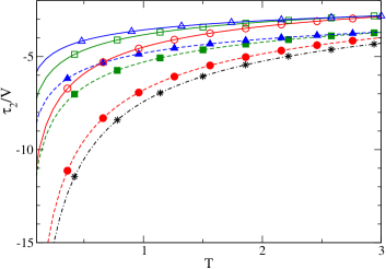
Figure 1: Second cluster integral divided by the volume for a fluid confined in a spherical pore. Different values of $\nu$ corresponds to circles ($\nu=6$), squares ($\nu=9$) and triangles ($\nu=12$). Continuous lines show results for $R=2$, dashed lines are for $R=20$ and dot-dashed is for the bulk system (only $\nu=6$ is shown).

As an example of the obtained results in Fig. 1 we plot the dependence with $T$ of the second cluster integral for the soft-sphere IPL fluid confined in a spherical pore. Curves show different values of the exponent and of the cavity radius. In the plot the natural units for $T$ were used i.e. $T$ is measured in $\alpha/k_{\textrm{B}}$ units.

IV Results: Surface tension

We consider the open system at low density confined by planar, spherical or cylindrical walls and truncate Eq. (8) at second order to obtain $\beta\Omega=-zV-z^{2}\frac{1}{2}\tau_{2}$. Therefore the first consequence of our calculus on $\tau_{2}$ is that the grand-free energy of the system contains the expected terms linear with volume and surface area. These terms are identical for the three studied geometries. At planar geometry, no extra term exist as symmetry implies for all $\tau_{i}$. In the case of spherical confinement a term linear with total normal curvature of the surface $2A/R\propto R$ does not appear at order $z^{2}$ but it should exist at higher ones. A term linear with quadratic curvature $A/R^{2}\propto\textrm{constant}$ exists. Extra terms that scale with negative powers of $R$ were also found. A logarithmic term proportional to $\ln R$ was recognized only for $\nu=6$. The cylindrical confinement is similar to the spherical case, thus we simply trace the differences: even that Gaussian curvature is zero in this geometry, a term linear with $A/R^{2}\propto L/R$ was found. The existence of a logarithmic term for $\nu=6$ was verified, in this case it was proportional to $L\ln R/R$.

For bulk homogeneous system the pressure and number density are $\beta P=z+z^{2}b_{2}$ and $\rho_{\textrm{b}}=z+z^{2}2b_{2}$ (subscript b refers to the bulk at the same $T$ and $\mu$). On the other hand, the surface tension is(Urrutia, 2014a)

$$\beta\gamma=-\frac{\Delta\tau_{2}}{2A}z^{2}=-\frac{\Delta\tau_{2}}{2A}\rho_{\textrm{b}}^{2}\>,$$ (31)

that are exact up to $\mathcal{O}(z^{3})$ and $\mathcal{O}(\rho_{\textrm{b}}^{3})$. By collecting results from Eqs. (12,23,24) and (26), and replacing in (31) one obtains the exact expression for planar and spherical walls and an approximated expression for cylindrical walls, up to the mentioned order in density. It yields $\gamma=a_{2}T\rho_{\textrm{b}}^{2}$ for the planar case. When lower order terms in $R^{-1}$ are retained for curved walls it is found,

$$\gamma_{\textrm{s}}=\left[a_{2}-\frac{c_{2}}{4\pi R^{2}}-\frac{d_{2}}{4\pi R^{3}}+\mathcal{O}\left(R^{-4}\right)\right]T\rho_{\textrm{b}}^{2}\>,$$ (32)

$$\gamma_{\textrm{c}}=\left[a_{2}-\frac{3c_{2}}{32\pi R^{2}}+\mathcal{O}\left(R^{-3}\right)\right]T\rho_{\textrm{b}}^{2}\>.$$ (33)

For the special case $\nu=6$ we should replace $c_{2}$ with $c_{l,2}\ln R$ ($d_{2}\neq 0$ only if $\nu=7$).

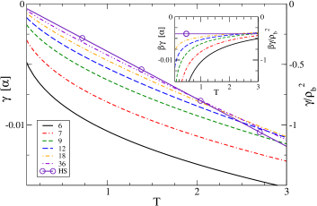
Figure 2: Fluid/wall surface tension in the case of a planar wall; we fix $\rho_{\textrm{b}}=0.1$ and consider various $\nu$ values. From bottom to top (at low temperatures) $\nu$ increases. Curves correspond to $\nu=6,7,9,12,18,36$ and to HS ($\nu\rightarrow\infty$).

In Fig.2 it is shown the surface tension of the gas confined by a planar wall for different values of $\nu$. Scale on the right shows $\gamma/\rho_{\textrm{b}}^{2}$, which is independent of density. All cases show $\gamma<0$, which is consistent with a repulsive potential and a monotonous decreasing behavior of $\gamma$ with $T$. In the limit $\nu\rightarrow\infty$ we obtain the asymptotic curve, which is a straight-line in coincidence with the HS result. In the inset it is shown $\beta\gamma$. There, asymptotic behavior for large $T$ corresponds to the constant value HS result and the hardening of curves with increasing $\nu$ is apparent. We note that several curves cross the HS limiting line and also that lines of different hardness intersect. This shows that softer potential may produce both smaller surface tension than harder potentials (at low temperature) but also larger surface tension than harder potentials (at high temperature). In Table 1 we present the dependence of $\gamma$ with temperature for planar walls.

$\nu$	$-\gamma/\rho_{\textrm{b}}^{2}$	$k/\rho_{\textrm{b}}^{2}$	$-k/\gamma$
$6$	$1.052T^{1/3}$	$0.0982$	$0.09$
$7$	$0.812T^{3/7}$	$0.107T^{1/7}$	$0.13$
$8$	$0.696\sqrt{T}$	$0.0593T^{1/4}$	$0.08$
$9$	$0.629T^{5/9}$	$0.0438T^{1/3}$	$0.07$
$12$	$0.532T^{2/3}$	$0.0290\sqrt{T}$	$0.053$
$18$	$0.467T^{7/9}$	$0.0221T^{2/3}$	$0.047$
$36$	$0.423T^{8/9}$	$0.0185T^{5/6}$	$0.042$
$\infty$	$0.393T$	$0.0164T$	$0.042$

Table 1: Dependence of planar surface tension and bending rigidity with temperature for some $\nu$ values. We fix $\alpha=k_{\textrm{B}}=1$. The ratio $-k/\gamma$ was evaluated at $T=1$.

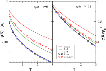
Figure 3: Surface tension of the fluid confined by spherical walls at $\rho_{\textrm{b}}=0.1$ (for both concave and convex shapes) and at various radii. At the left we plot the case $\nu=6$, at right the case $\nu=12$. The planar limit and cylindrical cases are also shown for comparison.

In the case of spherical walls the curvature dependence of the surface tension is plotted in Fig. 3. There, results for the $\nu=6$ (softer) and $\nu=12$ (harder) systems as a function of temperature are shown for different values of $R$. Again we found that surface tension is negative and decreases with $T$, which are characteristic signatures of repulsive interactions. Surface tension becomes larger at smaller radius and at $R\gtrsim 5$ is well described by the planar wall limit. A comparison of cases $\nu=6$ and $\nu=12$ shows that the sensitiveness of $\gamma$ with the radius is larger at softer potential.

Figure 3 is also related with the excess surface adsorption $\Gamma_{A}=\left(\left\langle n\right\rangle-\left\langle n\right\rangle_{\textrm{b}}\right)/A$. Series expansion of $\Gamma_{A}$ up to order $z^{2}$ and $\rho_{\textrm{b}}^{2}$ are: $\Gamma_{A}=z^{2}\Delta\tau_{2}/A$$=\rho_{\textrm{b}}^{2}\Delta\tau_{2}/A$. Thus, up to the order of Eq. (32) it is

$$\Gamma_{A}=-2\gamma/T\>,$$ (34)

showing that curves of $\gamma(R)$ also plot $-\Gamma_{A}T/2$. Naturally, the same apply to the planar case shown in Fig. 2 and to the cylindrical one. It must be noted that $\gamma(R)$ and $\Gamma_{A}$ depend on the adopted surface of tension that we fixed at $r=R$ where external potential goes from zero to infinity. This fixes the adopted reference region characterized by measures $V$, $A$, and $R$. The effect of introducing a different reference region on $\gamma(R)$ was systematically studied in Refs. (Urrutia, 2014a, 2015; Reindl et al., 2015) and will be briefly discussed in Sec. V.

V Results: Bending and Gaussian rigidities

On the basis of our results the expansion given in Eqs. (1, 2) is adequate for $\nu>6$ but not if $\nu=6$. For $\nu>6$, we found $\gamma\delta=\mathcal{O}(\rho_{\textrm{b}}^{3})$,

$$k = \frac{\pi}{192}\Gamma\left(1-\frac{6}{\nu}\right)\,T^{1-\frac{6}{\nu}}\,\rho_{\textrm{b}}^{2}+\mathcal{O}(\rho_{\textrm{b}}^{3})\>,$$ (35)

$$\bar{k} =- \frac{\pi}{288}\Gamma\left(1-\frac{6}{\nu}\right)\,T^{1-\frac{6}{\nu}}\,\rho_{\textrm{b}}^{2}+\mathcal{O}(\rho_{\textrm{b}}^{3})\>.$$ (36)

Again, if we replace using the identity $\beta^{q}\Gamma\left(1-q\right)\rightarrow-qC_{q}(0)$ these expressions coincide with those found recently for the Lennard-Jones fluid, but with a different definition for $C_{q}(0)$.(Urrutia and Paganini, 2016)

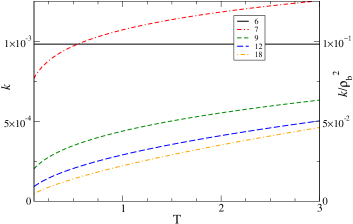
Figure 4: Fluid/wall bending rigidity $k$ as a function of temperature. We fix $\rho_{\textrm{b}}=0.1$ and consider various $\nu$ values. Curves correspond to $\nu=6,7,9,12,18$. The Gaussian rigidity $\bar{k}$ was not plotted because $\bar{k}=-0.66\boldsymbol{k}$ [see Eq. (37)].

In Fig. 4 the bending rigidity constant $k$ is presented as a function of temperature for different values of hardness parameter $\nu$. It is a positive increasing function of $T$ and is smaller for higher $\nu$. The case $\nu=6$ is different because the $\ln R$ term. Gaussian rigidity $\bar{k}$ is a negative decreasing function of $T$ and is higher for higher $\nu$. In Table 1 we present the numerical coefficients of the bending rigidity to show order of magnitude of $k\left(T\right)$. Besides, the relative weight of $k$ in surface tension is shown in last column. We observe that $k$ is smaller than $\gamma$ but may be as large as $0.13\times\gamma$ (case $\nu=7$ and $T=1$). The order $R^{-3}$ term in Eq. (1) corresponds to $\mathscr{C}=-\frac{\pi}{96}\rho_{\textrm{b}}^{2}$ for $\nu=7$ and is zero otherwise. It is interesting to calculate the quotient between $k$ and $\bar{k}$, and also the quotient of the next to $R^{-1}$ term in $\gamma$ between spherical and cylindrical cases. For all $\nu>6$ one finds

$$k/\bar{k} = -3/2\>,$$ (37)

$$2\frac{2k+\bar{k}}{k} = 8/3\>.$$ (38)

Remarkably, they are universal values in the sense that are independent of both $\nu$ and the state variable $T$. In the last ratio, the left-hand side of equation is independent of the assumptions of a Helfrich-based expression for $\gamma(R)$, and therefore it still applies if Eqs. (1,2) were wrong.

For non-short-ranged interactions as in the case of $\nu=6$ the logarithmic term makes Helfrich expansion(Helfrich, 1973) of $\gamma(R)$ in power of $R^{-1}$ no longer valid. Thus, for $\nu=6$ instead of the Eqs. (1,2), one obtains for the spherical and cylindrical walls

$$\gamma_{\textrm{s}}(R) = \gamma-\frac{2\gamma\delta}{R}+\left(2k+\bar{k}\right)\frac{\ln R}{R^{2}}+\mathcal{O}(R^{-2})\>,$$ (39)

$$\gamma_{\textrm{c}}(R) = \gamma-\frac{\gamma\delta}{R}+k\frac{\ln R}{2R^{2}}+\mathcal{O}(R^{-2})\>,$$ (40)

where bending and Gaussian rigidities were identified with the next order terms beyond $\gamma\delta$. We found

$$k=\frac{\pi}{32}\rho_{\textrm{b}}^{2}+\mathcal{O}(\rho_{\textrm{b}}^{3})\>\>\>\textrm{ and }\>\>\>\bar{k}=-\frac{\pi}{48}\rho_{\textrm{b}}^{2}+\mathcal{O}(\rho_{\textrm{b}}^{3})\>\>.$$ (41)

In this case both rigidities are temperature independent. The advent of $\ln R$ terms in Eqs. (39,40) demand to revise the invariance under the change of reference. $A\gamma_{\textrm{s}}(R)$ produces in $\Omega$ a term $\left(2k+\bar{k}\right)\ln R$, which is invariant and $A\gamma_{\textrm{c}}(R)$ produces in $\Omega$ a term $k\ln R/R$, which is also invariant. Both terms are invariant under the change of reference. Thus, for $\nu=6$ both rigidities $k$ and $\bar{k}$ are invariant under the change of reference system.

Even for $\nu=6$ we find for the ratios of curvatures the universal results given in Eqs. (37,38). In fact, the origin of these fundamental values is purely geometrical and was obtained previously for HS, square well, and Lennard-Jones, potentials.(Urrutia, 2014a; Urrutia and Paganini, 2016) Thus, essentially any pair interaction potential between particles produce the same value for the ratio $k/\bar{k}$ at low density. This result is in line with that found numerically using a second-virial approximation DFT.(Reindl et al., 2015) The same geometrical status claimed for $k/\bar{k}$ corresponds to the result $\gamma\delta=0+\mathcal{O}(\rho_{\textrm{b}}^{3})$ that is directly derivable from Eqs. (23,24,25) and applies to essentially any pair potential.

Accuracy of truncation in the low curvature expansion

Based on the exact universal relation Eq. (37) we analyze the consequences of truncate higher order curvature terms in $\gamma(R)$ and discuss some particular aspects concerning soft-spheres. We drop terms beyond $k$ and $\bar{k}$ and use Eq. (37) to rewrite surface tension as a function of only one rigidity constant, e.g., $\bar{k}$,

$$\gamma_{\textrm{s}}(R) = \gamma-\frac{2\gamma\delta}{R}-2\frac{\bar{k}}{R^{2}}\ell\>,$$ (42)

$$\gamma_{\textrm{c}}(R) = \gamma-\frac{\gamma\delta}{R}-\frac{3\bar{k}}{4R^{2}}\ell\>,$$ (43)

where $\ell=1$ or $\ell=\ln R$ as appropriate (e.g., for IPL if $\nu>6$ then $\ell=1$ and if $\nu=6$ then $\ell=\ln R$). Now, we look for a simple relation that linking the properties of a fluid in a spherical and cylindrical confinement (the same fluid under the same thermodynamic conditions $T$, $\mu$) enables to measure accurately intrinsic curvature-related properties. We focus on that producing the same surface tension,

$$\gamma_{\textrm{s}}(R_{\textrm{s}})=\gamma_{\textrm{c}}(R_{\textrm{c}})\>;$$ (44)

i.e., for a spherical cavity with a given radius $R_{\textrm{s}}$ we obtain the radius of the cylindrical cavity producing the same surface tension. Following Eqs. (42,43) and including terms of $\mathcal{O}\left(\rho_{b}^{2}\right)$, this surface isotension condition gives

$$R_{\textrm{c}}^{2}=0.375\,R_{\textrm{s}}^{2}\>,$$ (45)

for $\ell=1$ (the case $\ell=\ln R$ does not yield a simple analytic result).

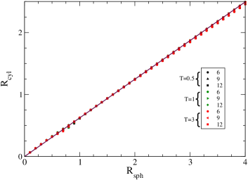
Figure 5: Relation between the radii under the iso-tension condition. Temperatures $T=0.5,1,3$ are drawn in black, green, and red symbols, respectively, but are difficult to distinguish in the plot. The straight line corresponds to Eq. (45).

This is a remarkable simple relation. To test the accuracy of the $R_{\textrm{c}}\leftrightarrow R_{\textrm{s}}$ relation beyond the truncation of higher-order terms in Eqs. (42,43) we solved numerically Eq. (44) with the exact $\gamma_{\textrm{s}}(R_{\textrm{s}})$ and a high-order truncation for $\gamma_{\textrm{c}}(R_{\textrm{c}})$ (we include contribution up to $C_{10/\nu}$). In Fig. 5 are shown the obtained results for the iso-tension relation between the radii of cylindrical and spherical confinements for different hardness parameter $\nu$ and temperatures. The plot shows that linear behavior predicted by Eq. (45) is very robust applying for all $\nu\geq 6$ and for a broad range of temperatures and radii. It also checks the robustness of approximate Eqs. (42,43) that would be good approximations for any fluid at low density.

Using Eq. (34) we infer that the relation between $R_{\textrm{c}}$ and $R_{\textrm{s}}$ also apply to the surface isoadsorption $\Gamma_{\textrm{c}}(R_{\textrm{c}})=\Gamma_{\textrm{s}}(R_{\textrm{s}})$ condition. The isotension-isoadsorption relation Eq. (45) is the consequence of purely geometrical aspects and thus applies to a large variety of fluids independently of the details of the interaction potentials. At finite and small value of $\rho_{\textrm{b}}$ and large enough radius the term $\gamma\delta\propto\rho_{\textrm{b}}^{3}$ should drive the relation between $R_{\textrm{c}}$ and $R_{\textrm{s}}$. In such case the slope change according to $R_{\textrm{c}}^{2}=0.25\,R_{\textrm{s}}^{2}$. This behavior is apparent in Ref. (Reindl et al., 2015) [see Fig. 4(a) therein]. Through the measure of adsorption isotherms (using for example molecular dynamics or Montecarlo simulations) we propose that relation $\Gamma_{\textrm{c}}(R_{\textrm{c}})=\Gamma_{\textrm{s}}(R_{\textrm{s}})$ and Eq. (45) are valuable tools to evaluate the accuracy of different approximations and the importance of $\mathcal{O}\left(R^{-2}\right)$ terms in the curvature dependence of the adsorption and surface tension for low-density fluids.

It is interesting to compare the relation $k=-3\bar{k}/2$ with that used in the context of the morphometric approach, where the bending rigidity identified with a quadratic term in the free energy is dropped.(Reindl et al., 2015) To this end we use the same interface convention adopted above and focus on low density behavior. The morphometric approach fix $k=0$ in Eqs. (1) and (2) for any density, giving

$$\gamma_{\textrm{s}}(R) \approx \gamma-\frac{2\gamma\delta}{R}+\frac{\bar{k}}{R^{2}}\ell\>,$$ (46)

$$\gamma_{\textrm{c}}(R) \approx \gamma-\frac{\gamma\delta}{R}\>,$$ (47)

which must be compared with Eqs. (42) and (43) which are exact up to order $\ell R^{-2}$. Under the morphometric approximation the correction to $\gamma_{\textrm{s}}$ produced by the term $R^{-2}$ is opposite in sign to the real one and the inaccuracy introduced in the approximation of $\gamma_{\textrm{s}}$ has the same order of that introduced in $\gamma_{\textrm{c}}$. Then, it is preferable to fix $k\approx 0$ and $\bar{k}\approx 0$ to obtain both simpler expressions and more accurate results for $\gamma_{\textrm{s,c}}$ than those based on morphometric Eqs. (46) and (47). Besides, at order $\rho_{\textrm{b}}^{2}$ morphometric approximation yields that $\gamma_{\textrm{c}}(R_{\textrm{c}})=\gamma_{\textrm{s}}(R_{\textrm{s}})$ never happens which confirm its sensibility to high order curvature terms.

As was mentioned the obtained results pertain to a reference surface that coincides with the position of zero-to-infinite wall interaction. The adopted reference surface has several advantages. For example, for the ideal gas it gives the beautifully simple relation $\Omega=-PV$ and $\gamma=\gamma\delta=k=\bar{k}=0$ while for shifted surfaces the free energy $\Omega$ becomes unnecessarily complicated. Further, several universal relations only apply under the adopted convention as the low density behavior $\gamma=\mathcal{O}(\rho_{\textrm{b}}^{2})$, $k=\mathcal{O}(\rho_{\textrm{b}}^{2})$ , $\bar{k}=\mathcal{O}(\rho_{\textrm{b}}^{2})$, $\gamma\delta=\mathcal{O}(\rho_{\textrm{b}}^{3})$, the surface tension and adsorption relation Eq. (34), the rigidity constants ratios given in Eqs. (37) and (38), and isotension Eq. (45). Even more, it has been shown that the adopted reference provides the more sensible condition to measure higher-order curvature terms in free energy.(Reindl et al., 2015) Beyond these qualities, once the properties are obtained on a given convention, one can transform to different shifted surfaces by simple rules that linearly combines $P$, $\gamma$, $\gamma\delta$, etc.(Urrutia, 2014a)

VI Summary and Conclusions

The use of virial series for confined fluids is an unusual approach that allows us to find new exact analytic results. This is a valuable feature that contributes to develop the theoretical framework of inhomogeneous fluids, a field where exact results are difficult to obtain and thus scarce.

In this work we utilized virial series at the lowest nontrivial order (up to order two in density and activity) to study the soft-sphere system confined by hard walls of planar, spherical and cylindrical shape. In the first and second cases we evaluate on exact grounds the second cluster integral with its full dependence on $R$, $T$, and $\nu$, while for cylindrical walls we found a quickly convergent expansion. With these analytic expressions we systematically analyze the effect of wall-curvature obtaining for the first time the expansion for planar and curved wall-fluid surface tension and its curvature components: Tolman length, bending and Gaussian rigidities. Even more, we evaluated the next-to constant rigidity term for spherical confinement, which is invariant under reference region transformation.

Our results for low density soft-spheres show that planar surface tension is a negative and monotonously decreasing function in $T$, as it is also the case for spherical and cylindrical walls. Furthermore, the effect of softening-hardening of the IPL pair potential is non-monotonous: for each $\nu$ there is a temperature where surface tension (and surface adsorption) coincides with that of HS system, for smaller temperatures $\gamma<\gamma_{HS}$ while for larger temperatures $\gamma>\gamma_{HS}$. This inversion appears to be in the same direction of that found for colloid-polymer mixtures where soft repulsion enhances the depletion mechanism.(Rovigatti et al., 2015) For the dependence on curvature it is observed that surface tension decreases with decreasing $R$ and that $\gamma<\gamma_{\textrm{c}}<\gamma_{\textrm{s}}$ at least for radii as smaller as $R\approx 0.5$.

In the case of curved walls we analyzed the small curvature expansion of surface tension and verify the existence of a logarithmic term when $\nu=6$. We calculated the exact expressions of bending and Gaussian rigidities as well as the simple relation between them. Bending rigidity is a positive increasing function of $T$, which decreases with rigidity $\nu>7$ but is constant if $\nu=6$.

We verified the validity of a set of relations that apply to any low-density fluid confined by smooth walls. They involve surface tension, surface adsorption, Tolman length, bending and Gaussian rigidities, and radii of curvature. These universal relations were found by adopting a particular choice of the reference region but concern to any interface convention once the reference transformation is done. Specially interesting was the surface isotension relation between $R_{\textrm{s}}$ and $R_{\textrm{c}}$ that provides an accurate mechanism to identify and measure high-order curvature dependence of surface tension. We expect that future development of approximate theoretical tools for confined fluids, including mixtures with macroscopic particles as colloids, may be benefited from these results.

Based on the Hadwiger theorem has been proposed that bending rigidity constant could be nearly zero(König et al., 2005) and thus would be unnecessary to include it in the expansion of $\gamma(R)$. Using the universal relations we show that the inaccuracy introduced by truncation of the bending rigidity term in $\gamma(R)$ is the same order of Gaussian rigidity term (at least for low density and hard walls), and therefore is not well justified from the numerical standpoint. Given that at least under the adopted interface convention the morphometric approximation does not comply with universal relations it could be better to ignore both rigidity constants than merely fix $k\approx 0$. In particular, for the soft-sphere system with $\nu=7$ the inaccuracy in $\gamma(R=1)$ introduced by the morphometric approximation is as large as $7\%$ (at $T=1$). Our results complement other recent works, showing that $k\neq 0$ for different fluids under different circumstances and suggesting that morphometric thermodynamics has to be used with caution.(Reindl et al., 2015; Urrutia and Paganini, 2016; Urrutia, 2014a; Hansen-Goos, 2014; Blokhuis and van Giessen, 2013; Blokhuis, 2013)

We think that arguments inducing to establish the absence of nonlinear terms in the free energy of fluids in thermodynamics and statistical mechanics should be revised at least when one recognizes that almost any real (finite-size) fluid system is in some sense confined.

Appendix A Some properties of $C_{q}$

We analyze $C_{q}$ at fixed $\tilde{\beta}$. When $\varepsilon\rightarrow+0$ for $0<q<1$ the function $C_{q}$ converges but it diverges for $q\geq 1$. In the convergent case we have

$$qC_{q}(0)=\tilde{\beta}^{q}q\Gamma\left(-q\right)=-\tilde{\beta}^{q}\Gamma\left(1-q\right)=-\tilde{\beta}C_{q-1}(0)$$

an identity used to obtain Eqs. (27,28,29), while for the nonconvergent case one can transform through $q\Gamma(-q,\varepsilon)=-\Gamma(1-q,\varepsilon)+e^{-\varepsilon}\varepsilon^{-q}$ to obtain(Abramowitz and Stegun, 1972)

$$qC_{q}(\varepsilon) = -\tilde{\beta}^{q}\Gamma(1-q,\tilde{\beta}\varepsilon)+\left(\tilde{\beta}\varepsilon\right)^{-q}\left(e^{-\tilde{\beta}\varepsilon}-1\right)\>,$$

$$= -\tilde{\beta}C_{q-1}(\varepsilon)+\left(\tilde{\beta}\varepsilon\right)^{-q}\left(e^{-\tilde{\beta}\varepsilon}-1+\frac{\tilde{\beta}\varepsilon}{q-1}\right).$$

The functional behavior of $C_{q}$ is simpler to analyze by introducing the function $F_{q}\equiv C_{q}(\varepsilon)\tilde{\beta}^{-q}$ that depends on $z=\mathbf{\tilde{\beta}}\varepsilon$, but not on $\tilde{\beta}$ and $\varepsilon$ separately. The series expansion for small and positive $z$ is

$$F_{q}=\Gamma(-q)+z^{-q}\sum_{{\scriptstyle k=1}}^{\infty}\frac{(-z)^{k}}{(q-k)k!}\>,$$ (49)

which applies to noninteger values $q>0$. On the other hand, in the case of integer positive values of $q$,

$$F_{q}=\frac{(-1)^{q}}{q!}\left[H_{q}-\gamma_{E}+\ln z^{-1}\right]+z^{-q}\sum_{\stackrel{{\scriptstyle{\scriptstyle k=1}}}{{{\scriptstyle k\neq q}}}}^{\infty}\frac{(-z)^{k}}{(q-k)k!}\>,$$ (50)

where $\gamma_{\textrm{E}}$ is the Euler number and $H_{q}$ is the harmonic number of order $q$ (for the lowest $q$ we have $H_{1}=1$, $H_{2}=1.5$). Thus, $F_{q}\approx z^{1-q}$ for $q>1$ (and $q$ noninteger), but $F_{q}\approx\ln z^{-1}$ if $q=1$. Moreover, a term proportional to $\ln z^{-1}$ appears for every integer value $q\geq 1$. On the opposite, for large values of $z>0$ we have the following expansion:

$$F_{q} = e^{-z}z^{-q}\left(\frac{1}{z}-\frac{q+1}{z^{2}}+\frac{(q+1)(q+2)}{z^{3}}\right.$$ (51)

$$\left.-\frac{(q+1)(q+2)(q+3)}{z^{4}}+...\right)\>.$$

The asymptotic behavior for small (and positive) values of $q$ and fixed $z$ is

$$qF_{q}=-1+\mathcal{O}(q)\>,$$

which reproduces the HS result.

Appendix B Hard core $C_{q}$

When the pair interaction between particles is defined as $\phi(r\leq\sigma)=+\infty$ and by the IPL given in Eq. (19) for $r>\sigma$ we obtain $C_{m+1,\nu}=-\frac{1}{m+1}+\frac{1}{\nu}C_{q}$, where the first term on the right is the hard-core contribution and

$$C_{q}(\varepsilon) = \int_{\varepsilon}^{1}y^{-(1+q)}\left[\exp\left(-\tilde{\beta}y\right)-1\right]dy\>,$$

$$= \frac{1-\varepsilon^{-q}}{q}+\tilde{\beta}^{q}\left[\Gamma\left(-q,\tilde{\beta}\varepsilon\right)-\Gamma\left(-q,\tilde{\beta}\right)\right]\>.$$

This relation applies to both repulsive ($\tilde{\beta}>0$) and attractive ($\tilde{\beta}<0$) IPL potentials. In the last case it is convenient to replace $\tilde{\beta}^{q}$ by $(-1)^{q}\left|\tilde{\beta}\right|^{q}$.