Gravity’s rainbow: a bridge between LQC and DSR

Abstract

The doubly special relativity (DSR) theories are constructed in order to take into account an observer-independent length scale in special relativity framework. It is widely believed that any quantum theory of gravity would reduce to a DSR model at the flat limit when purely gravitational and quantum mechanical effects are negligible. Gravity’s rainbow is a simple generalization of DSR theories to incorporate gravity. In this paper, we show that the effective Friedmann equations that are suggested by loop quantum cosmology (LQC) can be exactly reobtained in rainbow cosmology setup. The deformed geometry of LQC then fixes the modified dispersion relation and results in a unique DSR model. In comparison with standard LQC scenario where only the geometry is modified, both geometry and matter parts get modified in our setup. In this respect, we show that the total number of microstates for the universe is finite which suggests the statistical origin of the energy and entropy density bounds. These results explicitly show that the DSR theories are appropriate candidates for the flat limit of loop quantum gravity.
PACS numbers: 04.60.Bc
Keywords: Phenomenology of Quantum Gravity, Doubly Special Relativity

1 Introduction

In the standard model of cosmology, the universe starts from the big bang singularity where the classical Einstein’s equations are no longer applicable. The Hubble parameter diverges when the size of the universe approaches zero at the singularity. Beside, the singularity is also consistently understandable from the matter part where the standard statistical mechanics formalism applies to the early radiation dominated universe: The energy density of the universe, determined by the standard Stefan-Boltzmann law, and the associated entropy density diverge at big bang singularity. The energy density is directly related to the Hubble parameter in standard Friedmann cosmology while the entropy density is proportional to the inverse of the size of the universe through the adiabatic evolution of the universe. Therefore, the divergences of the geometrical and thermodynamical quantities are consistent in standard early universe cosmology. But the big bang singularity remains as an unsolved problem: Both of the classical Einstein’s equations and standard thermostatistics cannot explain the state of the universe at such a high energy regime. Quantum gravity candidates such as loop quantum gravity and string theory suggest the existence of a minimum length scale (of the order of the Planck length) below of which no other length can be probed [1, 2]. The existence of this minimum length scale evidently prevents the big bang singularity in loop quantum cosmology (LQC) [3, 4] and string cosmology [5]. In LQC, the big bang singularity problem can be resolved in such a way that the singularity replaces with a quantum bounce [4]. The Hubble parameter gets a maximum and there is a nonzero minimum size for the universe at the bounce. Existence of this geometrical maximum bound on the Hubble parameter immediately implies a maximum bound for the energy density through the Friedmann equation. Also, a maximum entropy density bound arises through the adiabatic evolution of the universe since the universe has a nonzero minimum size in LQC. These bounds on the energy and entropy densities, however, are not naturally supported by the standard statistical mechanics formalism. This inconsistency is understandable: The statistical mechanics formalism should be of course modified in order to include quantum gravity (minimal length) effects when one considers the modified geometry of LQC for the geometric part of the Einstein’s equations. The question then arises: How the statistical mechanics would be modified in the context of LQC while it only deals with the quantization of the geometry and not the matter? To answer this question, we note that at the flat limit, with which we are interested in the context of statistical mechanics, the fundamental quantum theory of gravity such as loop quantum gravity would reduce to a deformed (doubly) special relativity (DSR) which supports the existence of minimum observer-independent length scale [6]. In the absence of the final and well-established quantum theory of gravity, one can do in reverse: starting from the standard special relativity and deform it in such a way that it includes an invariant length scale. This is the main idea of the DSR theories [7]. The statistical mechanics in DSR framework is widely studied and, interestingly, it is shown that the entropy and energy densities get maximum bounds in this setup [8]. In this respect, in Ref. [9], it is claimed that the modified geometry of LQC is consistent with the statistical mechanics based on DSR and not the standard special relativity (see also Ref. [10]). But this consistency has not been explicitly confirmed. In this paper, we reobtain the effective Friedmann equation of LQC in gravity’s rainbow (doubly general relativity) formalism which is a simple generalization of DSR theories to include gravity [11]. This result explicitly shows the relevance of the DSR theories for the flat limit of loop quantum gravity. Moreover, the quantum gravity modifications to the statistical mechanics formalism naturally arise in our setup. The maximum bounds on Hubble parameter, energy density, and entropy density are then completely understandable from both geometrical and thermodynamical point of views in our setup.

2 Gravity’s Rainbow Cosmology

In recent years, the idea of gravity’s rainbow [11] attracted some attentions specially in black hole physics [12] and cosmology [13]. In this section we briefly review the early radiation dominated universe cosmology in this framework.

The DSR theories are generally defined by the deformed dispersion relation

$$f^{2}(\lambda{E})\,E^{2}-g^{2}(\lambda{E})\,p^{2}=m^{2}\,,$$ (1)

where $\lambda$ is the invariant UV scale which signals the existence of a minimal observer-independent length scale in this setup. The different DSR models are determined by the different functional forms for $f(\lambda{E})$ and $g(\lambda{E})$. All of these models respect the correspondence principle as $\lim_{\lambda{E}\rightarrow 0}f,g=1$ while they have different behaviors at UV regime [14]. The Lorentz symmetry breaks at UV regime for some models [7] or is preserved by nonlinear action of the Lorentz group on the associated curved momentum space [15, 16, 17]. In contrast to the standard special relativity, defining the position space to be dual to the curved momentum spaces in DSR setup is highly nontrivial [18, 19]. In Ref. [19], the authors suggest a novel construction of the dual position space. It is claimed that the metric on the dual position space will be $ds^{2}=-f^{-2}dt^{2}+g^{-2}\delta_{ij}dx^{i}dx^{j}$ in order to have plane wave solution for the corresponding free field theory. The setup is then generalized to the curved spacetime to incorporate gravity which resulted in gravity’s rainbow or doubly general relativity [11]. The modified equivalence principle is then investigated that leads to the one parameter family of connections and curvature tensors and therefore one parameter family of Einstein’s equations (see Ref. [11] for more details)

$$G_{\mu\nu}(\lambda{E})=8\pi{G(\lambda{E})}\,T_{\mu\nu}(\lambda{E})\,,$$ (2)

where $G(\lambda{E})$ is the effective gravitational coupling constant at UV regime which should lead to the standard Newton’s constant $G_{0}$ at low energy regime as $\lim_{\lambda{E}\rightarrow 0}G=G_{0}$. For the case of the flat FLRW spacetime, the corresponding rainbow metric is given by [11]

$$ds^{2}=f^{-2}\Big{(}-dt^{2}+a^{2}(t)\,\delta_{ij}dx^{i}dx^{j}\Big{)}\,,$$ (3)

where we have assumed $f=g$ in the relation (1). This choice leads to the constant speed of light through the modified dispersion relation (1) as $c(\lambda{E})=g/f=c_{0}=1$ (in our units). Note that the DSR theories generally lead to the varying speed of light [22, 14]. Also the definition of speed of light in DSR theories is not unique (see Refs. [19, 20] for more details). In gravity’s rainbow formalism, the definition $c=g/f$ is more acceptable since it coincides with the speed of null signals defined by the associated rainbow metric as $ds^{2}=0$. Thus, our choice of $f=g$ has a physical consequence that the speed of light is constant even in the UV regime similar to the well-known original Magueijo-Smolin model [16]. We also assume that the gravitational coupling constant being the standard Newton’s constant such that $G=G_{0}$ as one usually assumes in the context of gravity’s rainbow. These choices for the speed of light and gravitational constant are reasonable since we would like to explore the relation between the rainbow cosmology and LQC and both the speed of light and gravitational coupling constant have their standard constant definitions in LQC. The matter part is determined by the perfect fluid energy-momentum tensor

$$T_{\mu\nu}=\rho\,{u_{\mu}u_{\nu}}+P\,(g_{\mu\nu}+u_{\mu}u_{\nu})\,,$$ (4)

where $\rho$ and $P$ are the energy density and pressure. The four velocity $u_{\mu}$ depends on $\lambda{E}$ as $u_{\mu}=(f^{-1},0,0,0)$ to respect the normalization relation $g^{\mu\nu}u_{\mu}{u_{\nu}}=-1$.

Substituting the metric (3) together with the energy-momentum tensor (4) into the Einstein’s equations (2), one finds the following deformed Friedmann and Raychaudhuri equations (see Ref. [21] for details)

$$H^{2}-2H{\dot{f}}f^{-1}+{\dot{f}}^{2}f^{-2}=\frac{\kappa}{3}\,f^{-2}\rho\,,$$ (5)

$${\dot{H}}+H{\dot{f}}f^{-1}+{\ddot{f}}f^{-1}=-\frac{\kappa}{6}\,f^{-2}(\rho+P)\,,$$ (6)

where $\kappa=8\pi{G_{0}}$. The deformed Bianchi identities, then give the following modified energy conservation relation

$${\dot{\rho}}+3(H-{\dot{f}}f^{-1})(\rho+P)=0\,.$$ (7)

Two of the three equations (5), (6), and (7) are independent which completely determine the dynamics of the universe in our setup.

3 LQC versus DSR

In relations (5), (6) and (7), the evolution is considered with respect to the cosmic time $t$, while $f$ depends on kinematical energy $E$ and is not an explicit function of $t$. Also, the energy density $\rho$ and pressure $P$ do not explicitly depend on $E$. More precisely, $E$ is the total kinematical energy of the particles at which the spacetime geometry is probed [11]. Thus, it depends on $t$ and therefore $f$ depends on $t$ implicitly. On the other hand, for the case of early radiation dominated universe, the energy density and pressure in (4) depend on temperature and therefore on $t$ through the adiabatic condition. But, referring to Eq. (2), how these thermodynamical quantities may depend on the energy scale $E$ at which the spacetime geometry is probed? The key is indeed the modified dispersion relation (1) which immediately leads to the modification of the density of states [9, 22, 23]. For the case of massless particles in our setup with $f=g$ and therefore $E=p$, the form of the associated density of states remains unchanged [23]. But it is important to note that depending on the functional form of $f$, a UV cutoff $E<\lambda^{-1}$ can arise which modifies the thermodynamical quantities through the ranges of the integrals over the momenta (see for instance Ref. [9]). Therefore, the energy-momentum tensor depends on $\lambda{E}$ as it is shown in (2). In summary, at least for the radiation dominated universe, the bridge between the kinematical energy of particles $E$ and the energy density $\rho$ is given by the temperature when one reasonably identifies the kinematical energy $E$ with the thermodynamical internal energy $U$ that is the statistical average of $E$ [21]. More precisely, this relation is indeed between the dimensionless quantities $\lambda{E}$ and $\frac{\rho}{\rho_{\max}}$. We therefore assume

$$\lambda{E}=\frac{\rho}{\rho_{\max}}\,,$$ (8)

where $\rho_{\max}$ is the maximum value of the energy density corresponding to the maximal kinematical energy $E=\lambda^{-1}$. This relation will be fixed explicitly in section 5 through statistical considerations.

Let us rewrite the Friedmann equation (5) and the energy conservation relation (7) in more appropriate forms

$$H^{2}=\frac{\kappa}{3}\,f^{-2}\rho+2H{\dot{f}}f^{-1}-{\dot{f}}^{2}f^{-2}\,,$$ (9)

$${\dot{\rho}}=-3\big{(}H-{\dot{f}}f^{-1}\big{)}\big{(}1+w(\rho)\big{)}\rho\,,$$ (10)

where we have substituted $w(\rho)=P(\rho)/\rho$. Note that the equation of state parameter $w$ is modified in rainbow cosmology since the density of states gets modified through the cutoff $E<\lambda^{-1}$ in this setup [9, 22] (see also section 5 of the present paper). At the low energy limit ($\lambda{E}\rightarrow 0$), $f\rightarrow 1$ and equations (9) and (10) reduce to their standard counterparts. The functional form of $f$ in (9) and (10) is however not explicitly fixed and, therefore, there are many Friedmann equations for the different choices of $f$ (see for instance Refs. [9, 11, 21]). There is no clear reason to prefer one set of equations from the others and it is natural to expect that the ultimate quantum theory of gravity finally fixes the functional form of $f$. In the absence of such a theory, we can refer to quantum gravity candidates such as loop quantum gravity and string theory. Indeed, the (fixed) deformed Friedmann equations are investigated in the frameworks of LQC [4] and string cosmology [5]. Taking the equivalence relation (8) into account, we can fix the functional form of $f$ by referring to these candidates. This is what we can do at least in the absence of full quantum gravity theory. Here we would like to fix $f$ by invoking the effective Friedmann equations that are suggested by LQC. Following the method we introduce in this paper, one can also fix the functional form of $f$ through the string cosmology setup [5].

For the case of flat FLRW universe, the modified Friedmann equation in LQC framework is given by [24]

$$H^{2}=\frac{\kappa}{3}\,\rho\Big{(}1-\frac{\rho}{\rho_{c}}\Big{)}\,,$$ (11)

where

$$\rho_{c}=\rho_{\max}=\frac{3}{8{\pi}G_{0}\alpha_{0}\gamma^{2}l_{{}_{\rm Pl}}^{2}}\,,$$ (12)

is the critical energy density which is also the maximum accessible energy density for the universe. This quantity coincides with the maximum energy density $\rho_{\max}$ that perviously has been defined in (8). The two dimensionless parameters $\gamma$ and $\alpha_{0}$, are the Barbero-Immirzi parameter and the minimum eigenvalue of the area operator [24] respectively. The Barbero-Immirzi parameter is fixed as $\gamma=0.2375$ through the black hole entropy calculation [25] and the minimum area eigenvalue is $\alpha_{0}=4\sqrt{3}\pi\gamma=5.166$ for the homogenous and isotropic models. Both of these parameters disappear at the classical limit $\rho\ll\rho_{\max}=0.41\rho_{{}_{\rm Pl}}$ where (11) coincides with the standard Friedmann equation. The energy conservation relation remains unchanged in LQC setup and for the case of radiation dominated universe is given by

$${\dot{\rho}}+4H\rho=0\,.$$ (13)

The modified Friedmann equation (11) is obtained from the unique representation of holonomy-flux algebra in LQC. We use this unique equation to fix the from of $f$ in the corresponding Friedmann equation (9) suggested by gravity’s rainbow formalism. To do this end, we use the chain rule ${\dot{f}}={\dot{\rho}}\frac{df}{d\rho}=-4H\rho\frac{df}{d\rho}$ where we have used (13). Substituting this into the right hand side of (9) and then substituting $H$ from (11) into the left hand side, after some manipulations, we obtain the following first order differential equation

$$4\rho\frac{df}{d\rho}+f=\Big{(}1-\frac{\rho}{\rho_{\max}}\Big{)}^{-\frac{1}{2}}\,,$$ (14)

for $f$. This equation has the exact solution

$$f=\frac{1}{4}\,\Big{(}\frac{\rho}{\rho_{\max}}\Big{)}^{-\frac{1}{4}}B_{\frac{\rho}{\rho_{\max}}}\Big{(}\frac{1}{4},\frac{1}{2}\Big{)}\,,$$ (15)

where $B_{x}(a,b)$ is the incomplete Beta function and the integration constant is fixed such that $f(\rho\rightarrow 0)=1$ in order to respect the correspondence principle. Substituting (15) into the relation (9), it is easy to obtain the modified Friedmann equation (11) that is suggested by LQC. Although the Friedmann equation is the same as that is suggested by LQC, note that our setup differs from the LQC scenario since the energy conservation relation (10) is different from the standard one (13). This is because of the fact that the matter part is not modified in LQC setup while it gets UV modifications in rainbow cosmology through the modified dispersion relation [23, 22] (see also section 5). For the case of radiation dominated universe, the modification to the matter part results in deformed equation of state parameter [23, 22]. Substituting (15) into the relation (10) gives the following expression for the equation of state parameter

$$w=\frac{4}{3}\Big{(}1-\frac{\rho}{\rho_{\max}}\Big{)}\,_{2}F_{1}\left(\frac{3}{4},1,\frac{5}{4},\frac{\rho}{\rho_{\max}}\right)-1\,,$$ (16)

where ${}_{2}F_{1}(a,b;c;x)$ is the Hypergeometric function. The above relation correctly reduces to the standard case at low energy regime as $\lim_{\frac{\rho}{\rho_{\max}}\rightarrow 0}w=w_{0}=\frac{1}{3}$.

Substituting from (8) into the relation (15) gives $f=\frac{B_{\lambda{E}}\left(\frac{1}{4},\frac{1}{2}\right)}{4(\lambda{E})^{\frac{1}{4}}}$ which leads to the following modified dispersion relation

$$\frac{B_{\lambda{E}}^{2}\left(\frac{1}{4},\frac{1}{2}\right)}{16\sqrt{\lambda{E}}}\big{(}E^{2}-p^{2}\big{)}=m^{2}\,,$$ (17)

through the general relation (1). Therefore, among all possible forms for the undetermined function $f$, the special form (15), leading to the modified dispersion relation (17), is selected by LQC setup. In other words, the modified dispersion relation (17) leads to the effective Friedmann equation that is suggested by LQC through the gravity’s rainbow formalism.

4 Cosmological Implications

In the standard setup of LQC, the geometrical part of the Einstein’s equations gets modification such that the Hubble parameter and the size of the universe (scale factor) get maximum and minimum bounds respectively. For the case of early radiation dominated universe, existence of these geometrical bounds immediately imply maximum energy and entropy density bounds for the matter sector. The matter sector is described by the standard statistical mechanics which does not predict these bounds. More precisely, the energy and entropy density bounds can be accommodated by the standard thermostatistics, but they do not naturally emerge in this framework. In Ref. [9], it is shown that the energy and entropy densities get maximum bounds when the DSR setup is applied to the statistical systems. It is then claimed that the statistical mechanics in DSR framework is consistent with the modified geometry suggested by LQC. This consistency will become clear in this paper since in our setup the geometrical modifications are exactly the same as the LQC scenario and furthermore the statistical mechanics setup naturally gets minimal length modifications through the modified dispersion relation (17) (see the next section). In this section, we study the cosmological implications of our setup and the associated statistical mechanics will be considered in the next section.

The conservation relation (13) gives the well-known solution $\rho=\rho_{0}a^{-4}$ for the energy density of the radiation dominated universe. Although the form of the dependence of the energy density to the scale factor is the same as the standard radiation dominated universe, it is important to note that the energy density has maximum in this setup as $\rho_{\max}=\rho_{0}a_{\min}^{-4}$ where $a_{\min}$ is the minimum size of the universe. Substituting this into the Friedmann equation (11) and then integrating the resultant equation gives the following solution for the scale factor

$$a=a_{\min}\left(1+\frac{4}{\alpha_{0}\gamma^{2}}\left(\frac{t-t_{b}}{t_{{}_{\rm Pl}}}\right)^{2}\right)^{\frac{1}{4}}\,,$$ (18)

where the integration constant is fixed such that at $t=t_{b}$, the scale factor approaches its minimum value, $a=a_{\min}$. In Eq. (18) we have also used the relation (12) and the fact that $G_{0}=t_{{}_{\rm Pl}}^{2}$ in our units. The energy density $\rho=\rho_{0}a^{-4}$ in terms of the cosmic time $t$ then can be easily obtained as

$$\rho=\rho_{\max}\left(1+\frac{4}{\alpha_{0}\gamma^{2}}\left(\frac{t-t_{b}}{t_{{}_{\rm Pl}}}\right)^{2}\right)^{-1}\,.$$ (19)

It is interesting to note that the solutions (18) and (19) are well-known results in LQC. The scale factor versus the cosmic time is plotted in figure (1(a)). The dashed lines in this figures show two standard separate solutions which are disconnected by a classically forbidden region. The left hand side dashed line corresponds to the contracting universe ending in a future singularity and the right hand side dashed line represents the expanding universe that starts from the past singularity. The solid curves however, shows the solution of (18) which shows that the universe in our setup (much similar to the LQC setup) bounces from a contracting phase $t<0$ to a re-expanding epoch $t>0$. The energy density versus the time is also plotted in figure (1(b)) where again the dashed lines represent the standard classical solutions corresponding to the contracting (the left hand side dashed line) and expanding (the right hand side dashed line) universes. These solutions are disconnected by a classically forbidden region and also both of them diverge at the big bang singularity in the standard cosmology. This classically forbidden region is replaced with a bounce in our setup and the energy density (19) (the solid curve) increases with time for $t<0$ and approaches its maximum value $\rho_{\max}=\rho_{0}a_{\min}^{-4}$ at $t=t_{b}=0$, then decreases for $t>0$ and finally coincides with its standard counterpart at $t\gg{t_{{}_{\rm Pl}}}$.

Substituting from (12) for $\rho_{\max}$, the minimum size of the universe will be

$$a_{\min}=\left(\frac{8\pi\alpha_{0}\gamma^{2}}{3}\right)^{\frac{1}{4}}\,l_{{}_{\rm Pl}}\,.$$ (20)

This result shows that the big bang singularity problem is resolved in our setup so that the singularity replaces with a bounce. This is because of the fact that the geometry of our setup is dictated by LQC scenario [4].

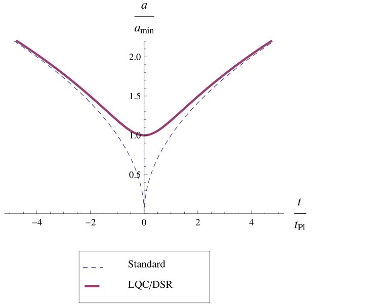
(a) Scale factor versus the cosmic time. The dashed lines represent two separate solutions of the standard radiation dominated universe while the solid curve shows the unique bouncing trajectory in our setup.

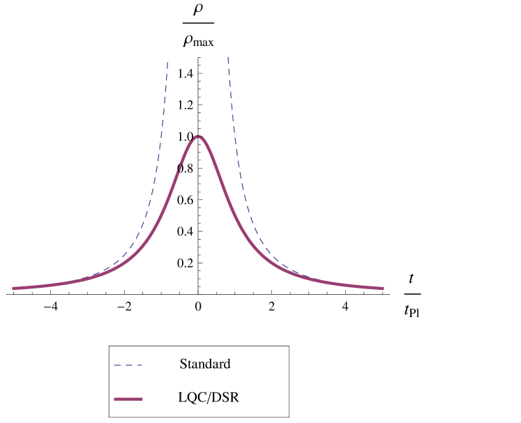
(b) Energy density versus the cosmic time. The dashed lines correspond to two separate solutions for the energy density in standard radiation dominated universe while the solid curve shows the corresponding unique solution in our setup.

Figure 1: The figures are plotted for $t_{{}_{\rm Pl}}=\frac{2}{\sqrt{\alpha_{0}}\gamma}$ and $t_{b}=0$.

Moreover, the existence of minimum size for the universe implies maximum bound for the entropy density through the adiabatic condition as

$$sa^{3}=S_{\rm tot}=\mbox{constant}\,,$$ (21)

where $S_{\rm tot}$ is the total entropy density of the universe. Substituting the scale factor from (18), the time evolution of the entropy density is then given by

$$s=s_{\max}\left(1+\frac{4}{\alpha_{0}\gamma^{2}}\left(\frac{t-t_{b}}{t_{{}_{\rm Pl}}}\right)^{2}\right)^{-\frac{3}{4}}\,,$$ (22)

where $s_{\max}=S_{\rm tot}a_{\min}^{-3}$ is the maximum value for the entropy density. The entropy density (22) versus the cosmic time is plotted in figure (2(a)). The dashed lines at the regions $t<0$ and $t>0$ show the two separate standard solutions for the entropy density which are disconnected by a classically forbidden region. Both of these solutions diverge at the big bang singularity (the point $t=0$ in figure (2(a))). Interestingly, in our setup, the classically forbidden region replaces with a bounce such that the entropy density (22) increases with time for $t<0$ until it approaches the maximum value $s_{\max}=S_{\rm tot}a_{\min}^{-3}$ at $t=t_{b}=0$ and then decreases with time and reduces to its standard counterpart for $t\gg{t_{{}_{\rm Pl}}}$.

While the equation of state remains unchanged in LQC setup (since only the geometry gets modified), it significantly modifies at UV regime in our setup through the deformed density of states. This is the crucial difference of our model with LQC at the cosmological setup. Substituting (19) into (16), we can easily obtain the time evolution of the equation of state parameter which is plotted in figure (2(b)). The negative values near the bounce $t=t_{b}=0$ signal repulsive force which is responsible for the singularity resolution in our setup. This repulsive force could naturally solve the horizon problem [11]. Furthermore, such a unstable accelerating phase has been interpreted as an inflationary phase in radiation dominated universe in Ref. [22].

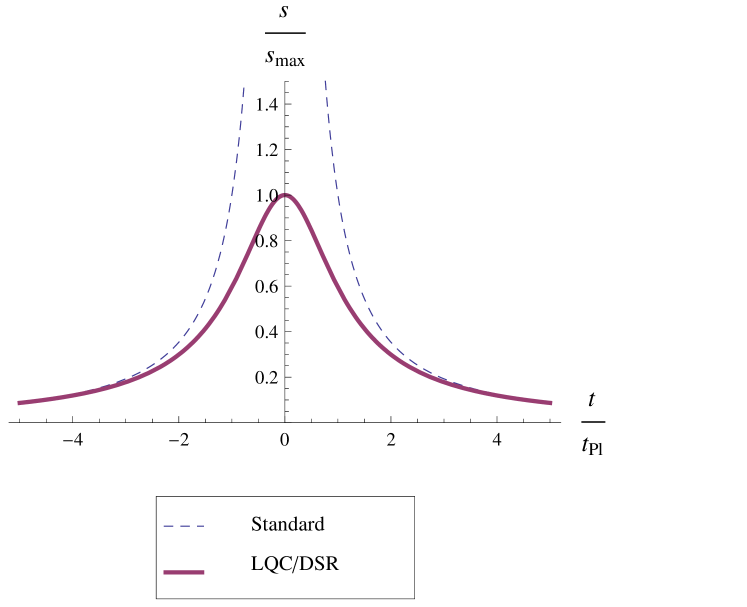
(a) Entropy density versus the cosmic time. Dashed lines represent two separate solutions for the entropy density of the standard radiation dominated universe. The solid curve shows the corresponding unique solution in our setup.

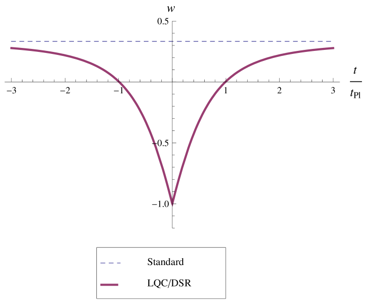
(b) Equation of state parameter versus the cosmic time. The equation of state parameter (the solid curve) becomes a function of time in our setup while it is constant in standard radiation dominated universe and also in LQC setup (the dashed line).

Figure 2: The figures are plotted for $t_{{}_{\rm Pl}}=\frac{2}{\sqrt{\alpha_{0}}\gamma}$ and $t_{b}=0$.

The spacetime singularity resolution that is emerged in our setup is a common feature of LQC scenario. More precisely, except the time-dependence of equation of state parameter (which is shown in figure (2(b))), all the results of this section are the same as those suggested by LQC. But, the advantage of our setup is that we can explore the statistical origin of the entropy and energy density bounds (see figures (1(b)) and (2(a))) while one cannot do so in LQC scenario. This is because of that fact that both of the geometrical and matter parts of Einstein’s equations get modified in gravity’s rainbow formalism while in LQC setup only the geometry is modified.

5 Entropy and Energy Density Bounds

In this section, we would like to study the thermostatistical properties of the early radiation dominated universe in our model defined by the modified dispersion relation (17). The key quantity is the number of states density which determines the total number of accessible microstates for the system under consideration. For the case of massless particles with which we are interested in early universe thermodynamics, the modified dispersion relation (17) gives $E=p$ and therefore the form of number of states density remains unchanged in our setup (see Refs. [9, 22, 23] for details). But, it is important to note that there is UV cutoff $E<\lambda^{-1}$ (or equivalently $p<\lambda^{-1}$ since $E=p$) in our setup and thus the modifications to the thermodynamical quantities arise at high energy regime $E\sim{\lambda^{-1}}\sim{E_{{}_{\rm Pl}}}$. The number of states density with energy in the interval between $E$ and $E+dE$ is given by [23]

$$d\Gamma=\frac{4\pi{V}g_{\star}}{h^{3}}E^{2}dE\,,$$ (23)

where $g_{\star}$ is the effective number of internal degrees of freedom and $h=2\pi$ in our units. The internal energy and the number of particles in local region with spatial volume $V$ are defined as

$$U=\int{n(E)}E\,d\Gamma\,,$$ (24)

$$N=\int{n(E)}\,d\Gamma\,,$$ (25)

where $n(E)=\left(\exp(E/T)\mp 1\right)^{-1}$ is the ensemble density and $(-)$ and $(+)$ signs are corresponding to the bosons and fermions respectively. The form of the ensemble density may be different at very high energy regime $E\sim{E_{{}_{\rm Pl}}}$ such that the standard definitions of bosons and fermions are no longer to be applicable. But, fortunately, following the method that is introduced in Ref. [9] we can address the main statistical properties of the universe without any attribution to ensemble density. The total number of microstates can be obtained by directly integrating the number of states density (23) as

$$\Gamma=\int{d\Gamma}=\frac{Vg_{\star}}{2\pi^{2}}\int_{0}^{\lambda^{-1}}E^{2}dE=\frac{g_{\star}}{6\pi^{2}}\left(\frac{V}{\lambda^{3}}\right)\,,$$ (26)

which interestingly is turned out to be finite. Note that the total number of microstates in the standard early universe statistical mechanics diverges since there is no upper bound for the kinematical energy and therefore the system could access more and more microstates with high and higher energies. The universe then goes to big bang singularity at $E\rightarrow\infty$ in the standard model of cosmology. The existence of the upper bound $E<\lambda^{-1}$ however prevents the big bang singularity from the statistical point of view such that the total number of potentially accessible microstates for the universe becomes finite. Having finite total number of microstates (26) immediately implies maximum bounds for the energy and entropy densities from the statistical point of view [9].

The entropy is directly determined by the number of microstates and therefore the emergence of finite total number of microstates (26) immediately leads to the following entropy density bound

$$s_{\max}=\ln{\Gamma}=\ln\left(\frac{V}{\lambda^{3}}\right)+\ln\left(\frac{g_{\star}}{6\pi^{2}}\right)\,,$$ (27)

for the early radiation dominated universe in our setup. From the relations (26) and (27) it is clear that, at high energy regime, the total number of microstates in local region with spatial volume $V$ is completely determined by the ratio $\frac{V}{\lambda^{3}}\sim\frac{V}{l_{{}_{\rm Pl}}^{3}}$. This result shows that one bit of information is determined by the fundamental volume $l_{{}_{\rm Pl}}^{3}$ in short distance regime.

Also, from the definition (25), it is clear that the total number of particles in a local region $V$ becomes finite as $N_{\max}=\int{d\Gamma}=\Gamma$ where we have used the relation (26). The associated total internal energy is defined by $U_{\max}=N_{\max}\times\frac{\int{E}d\Gamma}{\Gamma}=\int{E}d\Gamma$ which gives

$$\rho_{\max}=\frac{g_{\star}}{2\pi^{2}}\int_{0}^{\lambda^{-1}}E^{3}dE=\frac{g_{\star}}{8\pi^{2}}\lambda^{-4}\,,$$ (28)

where $\rho_{\max}=U_{\max}/V$ is the maximum accessible energy density for the universe. Thus, the existence of the upper bound for $E\leq\lambda^{-1}$ for the kinematical energy leads to the finite total number of microstates for the universe which immediately implies the maximum entropy and energy density bounds (27) and (28). These results explain the statistical origin of the entropy and energy density bounds which are shown in figures (1(b)) and (2(a)).

We are now adequately equipped to fix explicitly the equivalence relation (8) that we have assumed in section 3. From a thermodynamical point of view, the energy of the universe is given by the internal energy $U$ (or equivalently by the internal energy density $\rho=U/V$). On the other hand, from the kinematical point of view the energy is determined by the kinematical energy $E$. For the case of radiation dominated universe, the internal energy is directly related to the kinematical energy $U\sim{E}$. More precisely, the internal energy $U$ is the statistical average of the kinematical energy $E$ through the well-known definition (24). In our setup, there is an upper bound $E\leq\lambda^{-1}$ for the kinematical energy that nontrivially implies an upper bound (28) for the energy density (see also Ref. [9] where it is shown that the existence of an upper bound on kinematical energy does not necessarily imply an upper bound on the internal energy). The energy density should then approach its maximum value (28) when the kinematical energy approaches the maximum value $E_{\max}=\lambda^{-1}$. Therefore, in our setup, the critical energy density $\rho_{\max}$ (that is obtained in LQC setup) will be exactly equal to the maximum energy density $\rho_{\max}=U_{\max}/V$ which is obtained through statistical considerations. From (12) and (28), the observer-independent length scale $\lambda$ becomes fixed completely in terms of Barbero-Immirzi parameter $\gamma$ and effective number of degrees of freedom $g_{\star}$ as

$$\lambda=\left(\frac{\alpha_{0}\gamma^{2}g_{\star}}{3\pi}\right)^{\frac{1}{4}}\,l_{{}_{\rm Pl}}\,.$$ (29)

Substituting (29) into (20), gives the relation between the minimum size of the universe and the observer-independent length scale of DSR model (17) as

$$a_{\min}=\left(\frac{8\pi^{2}\rho_{0}}{g_{\star}}\right)^{\frac{1}{4}}\,\lambda\,.$$ (30)

The result (29) is interesting since it shows the explicit relation between the observer-independent length scale of DSR theories and Planck length as quantum of length that is suggested by LQC scenario. This relation also explicitly confirms that the DSR theories can be considered as the flat limit of loop quantum gravity [6]. Note that the minimum size of the universe (20) is completely fixed in LQC scenario since $\gamma=0.2375$ (through the black hole entropy calculation [25]) and $\alpha_{0}=4\sqrt{3}\pi\gamma=5.166$. But, the minimum observer-independent length scale $\lambda$ turned out to be directly related to the total number of particles that contribute to the energy content of the radiation dominated universe through the effective number of degrees of freedom $g_{\star}$. Bounds on $\lambda$ and therefore on $g_{\star}$ can be obtained through the methods that are introduced in Refs. [26].

6 Summary and Conclusions

Existence of a minimum measurable length scale is suggested by quantum gravity candidates such as loop quantum gravity and string theory. It is therefore widely believed that, at the flat limit when purely gravitational and quantum mechanical effects are negligible, the ultimate quantum theory of gravity would reduce to a deformed (doubly) special relativity (DSR) which supports the existence of minimum observer-independent length scale. Gravity’s rainbow (or doubly general relativity) is a simple generalization of DSR theories to include gravity in the semiclassical regime. In cosmological setup, different DSR models lead to the different Friedmann equations which include the effects of minimal observer-independent length scale. On the other hand, inspired by loop quantum gravity and string theory, the modified Friedmann equations are investigated in loop quantum cosmology (LQC) and string cosmology scenarios which also include the minimal length effects. In this paper, we have introduced a method by which one can fix the one-parameter family of Friedmann equations in rainbow cosmology by means of the deformed Friedmann equations that are suggested by the mentioned quantum gravity candidates. We applied the setup to the case of unique modified Friedmann equation suggested by LQC scenario. In this respect, among all possible DSR models, the DSR model defined by the modified dispersion relation (17) is selected by LQC. Moreover, this phenomenological derivation of LQC equations allowed us to explore the statistical origin of the energy and entropy density bounds that are arisen from the purely geometrical considerations in LQC scenario. This is because of the fact that while the statistical mechanics formalism remains unchanged in LQC scenario, it naturally gets quantum gravity modifications in our setup. We found that the total number of accessible microstates for the universe is finite which immediately implies the maximum bounds for the energy and entropy densities from the statistical point of view. The statistical considerations also completely fixed the relation between the quantum of spacetime in LQC setup in one side and the observer-independent length scale in DSR theories as (29) on the other side. These results explicitly show the relevance of the DSR theories for the flat limit of loop quantum gravity.

References

-
[1]
C. Rovelli and L. Smolin,
Nucl. Phys. B 442 (1995) 593
A. Ashtekar and J. Lewandowski, Class. Quantum Grav. 14 (1997) A55. -
[2]
D. J. Gross and P. F.
Mende, Nucl. Phys. B 303 (1988) 407
D. Amati, M. Ciafaloni and G. Veneziano, Phys. Lett. B 216 (1989) 41
L. Garay, Int. J. Mod. Phys. A 10 (1995) 145. -
[3]
M. Bojowald, Phys. Rev. Lett.
86 (2001) 5227
M. Bojowald, Class. Quantum Grav. 19 (2002) 2717. -
[4]
A. Ashtekar, T. Pawlowski
and P. Singh, Phys. Rev. D 74 (2006)
084003
A. Ashtekar, T. Pawlowski and P. Singh, Phys. Rev. Lett. 96 (2006) 141301. -
[5]
M. Gasperini and G.
Veneziano, Astropart. Phys. 1 (1993)
317
M. Gasperini, M. Maggiore and G. Veneziano, Nucl. Phys. B 494 (1997) 315
M. Gasperini and G. Veneziano, Phys. Rept. 373 (2003) 1. -
[6]
F. Girelli, E. R. Livine
and D. Oriti, Nucl. Phys. B 708
(2005) 411
C. Rovelli, arXiv:0808.3505 [gr-qc]
L. Smolin, arXiv:0808.3765 [hep-th]. -
[7]
G. Amelino-Camelia, Int. J.
Mod. Phys. D 11 (2000) 35
G. Amelino-Camelia, Nature 418 (2002) 34. -
[8]
J. Kowalski-Glikman,
Phys. Lett. A 299 (2002) 454
X. Zhang, L. Shao and B. -Q. Ma, Astropart. Phys. 34 (2011) 840
S. Das, S. Ghosh and D. Roychowdhury, Phys. Rev. D 80 (2009) 125036
S. Das and D. Roychowdhury, Phys. Rev. D 81 (2010) 085039
N. Chandra and S. Chatterjee, Phys. Rev. D 85 (2011) 045012
G. Amelino-Camelia, N. Loret, G. Mandanici and F. Mercati, Int. J. Mod. Phys. D 21 (2012) 1250052. - [9] M. A. Gorji, V. Hosseinzadeh, K. Nozari and B. Vakili, Phys. Rev. D 93 (2016) 064029.
- [10] G. Amelino-Camelia, M. M. da Silva, M. Ronco, L. Cesarini and O. M. Lecian, arXiv:1605.00497 [gr-qc].
- [11] J. Magueijo and L. Smolin, Class. Quantum Grav. 21 (2004) 1725.
-
[12]
Y. Ling, X. Li
and H. Zhang, Mod. Phys. Lett. A 22
(2007) 2749
A. F. Ali, Phys. Rev. D 89 (2014) 104040
A. F. Ali, M. Faizal and M. M. Khalil, JHEP 1412 (2014) 159
A. F. Ali, M. Faizal and M. M. Khalil, Nucl. Phys. B 894 (2015) 341
-
[13]
A. Awad, A. F. Ali
and B. Majumder, JCAP 1310 (2013)
052
R. Garattini and E. N. Saridakis, Eur. Phys. J. C 75 (2015) 343. - [14] M. Arzano, G. Gubitosi, J. Magueijo and G. Amelino-Camelia, Phys. Rev. D 92 (2015) 024028.
-
[15]
J. Kowalski-Glikman and
S. Nowak, Phys. Lett. B 539 (2002)
126
J. Kowalski-Glikman, Phys. Lett. B 547 (2002) 291
J. Kowalski-Glikman and S. Nowak, Class. Quantum Grav. 20 (2003) 4799. -
[16]
J. Magueijo and L. Smolin,
Phys. Rev. Lett. 88 (2002) 190403
J. Magueijo and L. Smolin, Phys. Rev. D 67 (2003) 044017. -
[17]
G. Amelino-Camelia, L.
Freidel, J. Kowalski-Glikman and L.
Smolin, Phys. Rev. D 84 (2011)
084010
G. Amelino-Camelia, Phys. Rev. D 85 (2012) 084034. -
[18]
S. Majid, Lect. Notes
Phys. 541 (2000) 227
A. A. Deriglazov, Phys. Lett. B 603 (2004) 124
A. A. Deriglazov and B. F. Rizzuti, Phys. Rev. D 71 (2005) 123515
S. Hossenfelder, Phys. Lett. B 649 (2007) 310. - [19] D. Kimberly, J. Magueijo and J. Medeiros, Phys. Rev. D 70 (2004) 084007.
-
[20]
P. Kosinski and P.
Maslanka, Phys. Rev. D 68 (2003)
067702
M. Daszkiewicz, K. Imilkowska and J. Kowalski-Glikman, Phys. Lett. A 323 (2004) 345
G. Amelino-Camelia, N. Loret and G. Rosati, Phys. Lett. B 700 (2011) 150. -
[21]
Y. Ling, JCAP
0708 (2007) 017
Y. Ling and Q. Wu, Phys. Lett. B 687 (2010) 103. - [22] S. Alexander, R. Brandenberger and J. Magueijo, Phys. Rev. D 67 (2003) 081301.
- [23] G. Santos, G. Gubitosi and G. Amelino-Camelia, JCAP 1508 (2015) 005.
- [24] A. Ashtekar and E. Wilson-Ewing, Phys. Rev. D 78 (2008) 064047.
- [25] K. A. Meissner, Class.c Quantum Grav. 21 (2004) 5245.
-
[26]
S. Das and E. C.
Vagenas, Phys. Rev. Lett. 101
(2008) 221301
P. Pedram, K. Nozari and S. H. Taheri, JHEP 1103 (2011) 093
S. Ghosh, Class. Quantum Grav. 31 (2014) 025025
S. Jalalzadeh, M. A. Gorji and K. Nozari, Gen. Rel. Grav. 46 (2014) 1632.