Bicollinear Antiferromagnetic Order, Monoclinic Distortion,
and Reversed Resistivity Anisotropy in FeTe as a Result of Spin-Lattice Coupling.

Abstract

The bicollinear antiferromagnetic order experimentally observed in FeTe is shown to be stabilized by the coupling $\tilde{g}_{12}$ between monoclinic lattice distortions and the spin-nematic order parameter with $B_{\rm 2g}$ symmetry, within a three-orbital spin-fermion model studied with Monte Carlo techniques. A finite but small value of $\tilde{g}_{12}$ is required, with a concomitant lattice distortion compatible with experiments, and a tetragonal-monoclinic transition strongly first order. Remarkably, the bicollinear state found here displays a planar resistivity with the “reversed” puzzling anisotropy discovered in transport experiments. Orthorhombic distortions are also incorporated and phase diagrams interpolating between pnictides and chalcogenides are presented. We conclude that the spin-lattice coupling discussed here is sufficient to explain the challenging properties of FeTe.

Introduction. The chalcogenide FeTe has long been considered an unusual member of the iron-based superconductors family intro ; dainat . Angle-resolved photoemission (ARPES) results zhang for this material revealed substantial mass renormalizations indicative of electrons that are more strongly interacting than in pnictides (see also akrap ). The absence of Fermi surface (FS) nesting instabilities was also conclusively established xia ; phlin . Moreover, using single-crystal neutron diffraction, the unexpected presence in FeTe of a “bicollinear” magnetic state was reported bao . This exotic antiferromagnetic (AFM) state is known as the E-phase in manganites CMR . Phenomenological approaches to rationalize the bicollinear state rely on Heisenberg $J_{1}$-$J_{2}$-$J_{3}$ models ma with the constraints $J_{3}>J_{2}/2$ and $J_{2}>J_{1}/2$, implying that the furthest distance coupling $J_{3}$ must be robust. Effective spin models ma ; bernevig are certainly valid descriptions after the distortion occurs, but they do not illuminate on the fundamental reasons for the bicollinear state stability lipscombe ; qinlong .

Upon cooling, experimentally it is known that the bicollinear state is reached via a robust first-order phase transition bao ; chen ; fobes , with a concomitant tetragonal ($\mathcal{T}_{\rm etra}$) to monoclinic ($\mathcal{M}_{\rm ono}$) lattice distortion. The reported lattice distortions in Fe_1.076Te and Fe_1.068Te are $\delta_{M}=|a_{M}-b_{M}|/(a_{M}+b_{M})\sim 0.007$  bao ($a_{M}$ and $b_{M}$ are the low temperature lattice parameters in the $\mathcal{M}_{\rm ono}$ notation). This distortion is comparable to the orthorhombic ($\mathcal{O}_{\rm rth}$) lattice distortion in BaFe₂As₂ huang $\delta_{O}=|a_{O}-b_{O}|/(a_{O}+b_{O})\sim 0.004$ (now with $a_{O}$ and $b_{O}$ the low temperature lattice parameters in the $\mathcal{O}_{\rm rth}$ notation). Since the lattice is considered a “passenger” in the properties of the pnictides, it may be suspected that it also plays a secondary role for chalcogenides.

Contrary to this reasoning, in this publication we argue that the lattice plays a more fundamental role in FeTe compounds than previously anticipated. Specifically, we construct a spin-fermion (SF) model where lattice and spins are coupled in a manner that includes the $\mathcal{M}_{\rm ono}$ distortion of FeTe. Using Monte Carlo techniques, we found a strong first-order $\mathcal{T}_{\rm etra}$ to $\mathcal{M}_{\rm ono}$ lattice transition upon cooling, as in experiments bao . Moreover, the bicollinear magnetic order spontaneously arises at the same critical temperature. Furthermore, this is achieved with a (dimensionless) spin-lattice coupling $\tilde{g}_{12}\gtrsim 0.10-0.25$ that is weak/intermediate in strength. Surprisingly, we also find the same puzzling reversed anisotropy in the low temperature resistivity reported recently reverse1 ; reverse2 , with the AFM direction more resistive than the ferromagnetic (FM), contrary to the behavior in pnictides.

Our study also includes the spin-lattice coupling $\tilde{g}_{66}$ that favors orthorhombicity although in this case the crystal’s geometry – with nearest-neighbors (NN) and next-NN (NNN) hoppings of similar strength and associated FS nesting – already favors the magnetic $(\pi,0)$ collinear state even without involving the lattice. Our analysis allows for an interpolation between pnictides, with collinear order, and chalcogenides, with bicollinear order, using the same hopping amplitudes, compatible with band structure calculations that give similar results for both materials DFT . In fact, we show that the high temperature regime displays a FS with the canonical hole and electron pockets, leading to the naive assumption that only $\mathcal{O}_{\rm rth}$ and $(\pi,0)$ spin order could be stabilized. However, our calculations explicitly show that strong first-order transitions can induce a low-temperature state with no precursors at high temperatures. In other words, in the absence of the spin-lattice coupling $\tilde{g}_{12}$ there is no transition to a bicollinear AFM state.

The presence of both itinerant and localized characteristics in neutron experiments for Fe_1.1Te igor suggest that the SF model provides a proper framework for iron tellurides. While in our effort the electronic interactions cannot be fully incorporated, the Hund coupling, crucial in the SF model, mimics a Hubbard $U$ by reducing double occupancy at each orbital. The importance of the Hund coupling has also been remarked within ARPES phlin . In these respects, our study has the same degree of accuracy as in previous successful descriptions of materials such as manganites CMR ; more-CMR .

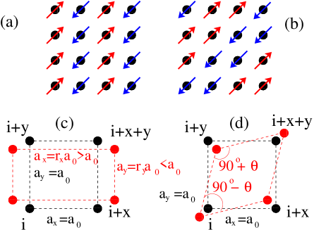
Figure 1: (color online) (a) The collinear $(\pi,0)$ AFM ordered state; (b) the bicollinear $(\pi/2,-\pi/2)$ AFM ordered state; (c) schematic drawing of the Fe lattice equilibrium position in the $\mathcal{T}_{\rm etra}$ (black symbols) and $\mathcal{O}_{\rm rth}$ (red symbols) phases (four Fe’s are indicated with filled circles and labeled by their site index ${\bf i}$); (d) Same as (c) but for the $\mathcal{M}_{\rm ono}$ case.

Model. The SF Hamiltonian used here is based on the original purely electronic model previously discussed BNL ; shuhua , supplemented by the addition of couplings to the lattice degrees of freedom shuhua13 ; chris :

$$H_{\rm SF}=H_{\rm Hopp}+H_{\rm Hund}+H_{\rm Heis}+H_{\rm Stiff}+H_{\rm SLO}+H_{\rm SLM}.$$ (1)

$H_{\rm Hopp}$ is the three-orbital ($d_{xz}$, $d_{yz}$, $d_{xy}$) tight-binding Fe-Fe hopping of electrons, with the hopping amplitudes selected to reproduce ARPES data [see Eqs.(1-3) and Table 1 of three ]. The undoped-limit average electronic density per iron and per orbital is $n$=4/3 three and a chemical potential in $H_{\rm Hopp}$ chris controls its value. The Hund interaction is $H_{\rm Hund}$=$-{J_{\rm H}}\sum_{{\bf i},\alpha}{{{\bf S}_{\bf i}}\cdot{{\bf s}_{{\bf i},\alpha}}}$, where ${{\bf S}_{\bf i}}$ are localized spins at site ${\bf i}$ and ${\bf s}_{{\bf i},\alpha}$ are itinerant spins corresponding to orbital $\alpha$ at the same site foot . $H_{\rm Heis}$ contains the NN and NNN Heisenberg interactions among the localized spins, with respective couplings $J_{\rm NN}$ and $J_{\rm NNN}$, and ratio $J_{\rm NNN}$/$J_{\rm NN}$ = 2/3 (any ratio larger than 1/2 leads to similar results below). The NN and NNN Heisenberg interactions are of comparable magnitude because in FeTe electrons hop from Fe to Fe via the intermediate Te atom at the center of Fe plaquettes Hubbard . $H_{\rm Stiff}$ is the lattice stiffness given by a Lennard-Jones potential to speed up convergence chris (see full expression in shuhua13 ).

Previous SF model investigations focused on the $\mathcal{T}_{\rm etra}$-$\mathcal{O}_{\rm rth}$ transition as in SrFe₂As₂ shuhua13 . The coupling of the spins with the $\mathcal{O}_{\rm rth}$ lattice distortion discussed in shuhua13 is given by $H_{\rm SLO}$=$-g_{66}\sum_{\bf i}\Psi^{NN}_{\bf i}\epsilon_{66}({\bf i})$ fernandes1 ; fernandes2 , where $g_{66}$ is the canonical $\mathcal{O}_{\rm rth}$ spin-lattice coupling only and the spin NN nematic order parameter is defined as

$$\Psi^{NN}_{\bf i}={1\over{2}}{{{\bf S}_{\bf i}}\cdot{({\bf S}_{\bf i+\bf y}+{\bf S}_{\bf i-\bf y}-{\bf S}_{\bf i+\bf x}-{\bf S}_{\bf i-\bf x})}},$$ (2)

where ${\bf x}$ and ${\bf y}$ are unit vectors along the $x$ and $y$ axes, respectively. This order parameter is 2 in the perfect ($\pi$,0) state shown in Fig. 1 (a). $\epsilon_{66}({\bf i})$ is the lattice $\mathcal{O}_{\rm rth}$ strain defined in terms of the positions of the As, Se or Te atoms with respect to their neighboring Fe. Its precise definition is shuhua13

$$\epsilon_{66}({\bf i})={1\over{4\sqrt{2}}}\sum_{\nu=1}^{4}(|\delta^{y}_{\bf i,\nu}|-|\delta^{x}_{\bf i,\nu}|),$$ (3)

where $\delta_{\bf i,\nu}=(\delta^{x}_{\bf i,\nu},\delta^{y}_{\bf i,\nu})$ ($\nu$=1,…,4) is the distance between Fe at ${\bf i}$ and one of its four neighbors As or Te (Fig. S1, Suppl. Sec. SuSe ). The As/Te atoms are allowed to move locally from their equilibrium position only along the $x$ and $y$ directions for simplicity. Both $\Psi^{NN}_{\bf i}$ and $\epsilon_{66}({\bf i})$ transform as the $B_{\rm 1g}$ representation of the $D_{\rm 4h}$ group under which $H_{\rm SF}$ is invariant.

The crucial novel term $H_{\rm SLM}$=$-g_{12}\sum_{\bf i}\Psi^{NNN}_{\bf i}\epsilon_{12}({\bf i})$ introduced here provides the coupling between the spin and the $\mathcal{M}_{\rm ono}$ lattice distortion kuo . The coupling constant is $g_{12}$ and the spin NNN nematic order parameter is defined as

$$\Psi^{NNN}_{\bf i}={1\over{2}}{{{\bf S}_{\bf i}}\cdot{({\bf S}_{\bf i+\bf x+\bf y}+{\bf S}_{\bf i-\bf x-\bf y}-{\bf S}_{\bf i+\bf x-\bf y}-{\bf S}_{\bf i-\bf x+\bf y})}}.$$ (4)

$\Psi^{NNN}_{\bf i}$ becomes 2 in the perfect ($\pi/2$,$-\pi/2$) state shown in Fig. 1 (b) moment . $\epsilon_{12}({\bf i})$ is the lattice $\mathcal{M}_{\rm ono}$ strain defined in terms of the Fe-Te/As distances $\delta_{{\bf i},\nu}$ as

$$\epsilon_{12}({\bf i})={1\over{8}}(|\delta_{{\bf i},2}|+|\delta_{{\bf i},4}|-|\delta_{{\bf i},1}|-|\delta_{{\bf i},3}|).$$ (5)

$\epsilon_{12}({\bf i})$ transforms as the $B_{\rm 2g}$ representation. For this reason we must use $\Psi^{NNN}_{\bf i}$, that also transforms as $B_{\rm 2g}$, in the product leading to $H_{\rm SLM}$ so that this term is invariant under the $D_{\rm 4h}$ group. This simple symmetry argument is the basic reason for why the bicollinear state is stabilized by the monoclinic distortion, as discussed below.

$H_{\rm SF}$ was studied here with the same Monte Carlo (MC) procedure employed before in shuhua13 (details in SuSe ). The range of couplings for $J_{\rm H}$, $J_{\rm NN}$, and $J_{\rm NNN}$ that we used was also extensively discussed before in shuhua ; shuhua13 (see SuSe as well). Our focus instead will be on a careful description of the new lattice coupling $\tilde{g}_{12}$. During the simulation the As/Te atoms can move locally away from their equilibrium positions on the $x$-$y$ plane, while the Fe atoms can move globally in two ways: (i) via an $\mathcal{O}_{\rm rth}$ distortion characterized by a global displacement $(r_{x},r_{y})$ from the equilibrium position $(x^{(0)}_{i},y^{(0)}_{i})$ of each iron with $r_{\alpha}=1+\Delta_{\alpha}$ ($\Delta_{\alpha}\ll 1$; $\alpha=x$ or $y$) [Fig. 1 (c)], and (ii) via a $\mathcal{M}_{\rm ono}$ distortion where the angle between two orthogonal Fe-Fe bonds is allowed to change globally to $90^{o}+\theta$ with the four angles in the $\mathcal{M}_{\rm ono}$ plaquette adding to $360^{o}$ so that the next angle in the plaquette becomes $90^{o}-\theta$, with $\theta$ a small angle [Fig. 1 (d)]. In addition, the localized (assumed classical) spins ${\bf S_{i}}$ and atomic displacements $(\delta^{x}_{{\bf i},\nu},\delta^{y}_{{\bf i},\nu})$ that determine the local $\mathcal{O}_{\rm rth}$ or $\mathcal{M}_{\rm ono}$ lattice distortion $\epsilon_{66}({\bf i})$ shuhua13 ; chris and $\epsilon_{12}({\bf i})$ are also evaluated via MC. In SuSe we provide the definitions of the spin and lattice susceptibilities $\chi_{S(k_{x},k_{y})}$, $\chi_{\delta_{O}}$, and $\chi_{\delta_{M}}$, and the dimensionless couplings $\tilde{g}_{66}$ and $\tilde{g}_{12}$.

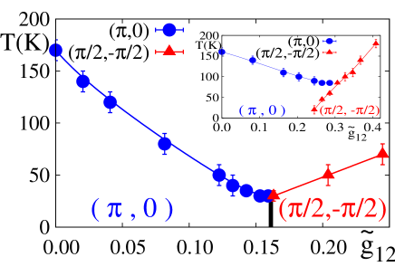
Figure 2: (color online) Phase diagram varying temperature along the straight line from $(\tilde{g}_{12},\tilde{g}_{66})=(0,0.24)$ to $(0.24,0)$, at $J_{\rm H}=0.1$ eV and $J_{\rm NN}$=$J_{\rm NNN}$=0. Inset: the same phase diagram but along the straight line from $(\tilde{g}_{12},\tilde{g}_{66})=(0,0.16)$ to $(0.40,0)$, at $J_{\rm H}=0.1$ eV, $J_{\rm NN}=0.012$ eV, and $J_{\rm NNN}=0.008$ eV. Blue circles (red triangles) denote $T_{\rm O}$ ($T_{\rm M}$) i.e. the transition temperatures to the $\mathcal{O}_{\rm rth}$/collinear ($\mathcal{M}_{\rm ono}$/bicollinear) phases.

Results. In real chalcogenides, both $B_{\rm 1g}$ and $B_{\rm 2g}$ magnetic fluctuations are expected to be present and the magnitude of their respective couplings to $\mathcal{O}_{\rm rth}$ and $\mathcal{M}_{\rm ono}$ distortions may depend on doping, replacing Te by Se, or adding extra irons as in Fe_1+yTe. In addition, weak $B_{\rm 2g}$ fluctuations may also exist in pnictides. For this reason, our study will be illustrated showing the MC phase diagrams varying temperatures and couplings in a wide range. Consider first the case $J_{\rm NN}=J_{\rm NNN}=0.$ One of our most important results is in Fig. 2. At the left, a realistic $T_{\rm O}^{max}\approx 170$ K is obtained for the transition that stabilizes the collinear/$\mathcal{O}_{\rm rth}$ state, with an $\mathcal{O}_{\rm rth}$ distortion $\delta_{O}\approx 0.004-0.008$, compatible with experiments bao and with previous studies shuhua13 . As $~{}\tilde{g}_{12}$ increases and $~{}\tilde{g}_{66}$ linearly decreases, then $T_{\rm O}^{max}$ naturally decreases. When $~{}\tilde{g}_{12}\approx 0.16$ and $~{}\tilde{g}_{66}\approx 0.08$, remarkably now the FeTe bicollinear/$\mathcal{M}_{\rm ono}$ phase appears at $T_{\rm M}$ (red triangles). At the right in Fig. 2 the critical temperature is $\sim 70$ K similarly as in FeTe experiments mizuguchi . Moreover, in the range shown, the monoclinic lattice distortions are small and compatible with experiments (for explicit values see Fig. S4 of SuSe ) comment-10K .

Why bicollinear order is stabilized? The reason is that with increasing $~{}\tilde{g}_{12}$, the nematic order parameter $\Psi^{NNN}_{\bf i}$ in $H_{\rm SLM}$ must develop a nonzero expectation value to lower the energy. In each odd-even site sublattice, $\Psi^{NNN}_{\bf i}$ favors a state with parallel spins along one diagonal direction and antiparallel in the other (equivalent to the collinear order but rotated by 45^o). The parallel locking of the two independent spin sublattices leads to the state in Fig. 1 (b) (or rotated ones).

As already explained, the purely fermionic SF model develops a collinear $(\pi,0)$ AFM ground state because of FS nesting tendencies in the tight-binding sector shuhua . Since spin and lattice are linearly coupled, an $\mathcal{O}_{\rm rth}$ distortion is induced even for an infinitesimal $\tilde{g}_{66}$. On the other hand, regardless of $\tilde{g}_{66}$, we observed that the coupling $\tilde{g}_{12}$ needed to stabilize the bicollinear/$\mathcal{M}_{\rm ono}$ state is finite because it must first “fight” the $(\pi,0)$ order tendencies. However, in practice this critical coupling is small $\sim 0.1$-$0.25$ and within the experimental range.

To analyze the universality of the Fig. 2 phase diagram we have also investigated the effect of adding NN and NNN Heisenberg couplings along the line from $(\tilde{g}_{12},\tilde{g}_{66})=(0,0.16)$ to $(0.40,0)$ (inset of Fig. 2). Qualitatively the results are similar. At $(0.40,0)$ in the inset, the largest value of $\tilde{g}_{12}$ considered in the present study, the $\mathcal{M}_{\rm ono}$ distortion is $\delta_{M}\approx 0.004$ still of the order of magnitude experimentally observed in FeTe bao . One interesting difference, though, between the two cases in Fig. 2 is the appearance in the inset of an intermediate region at $\tilde{g}_{12}\approx 0.28$ where upon heating a transition $\mathcal{M}_{\rm ono}$ to $\mathcal{O}_{\rm rth}$ is reached before the system eventually becomes paramagnetic. Experimentally it is indeed known that in Fe_1+yTe an intermediate $\mathcal{O}_{\rm rth}$ phase with incommensurate magnetic order exists between the $\mathcal{T}_{\rm etra}$ and $\mathcal{M}_{\rm ono}$ phases mizuguchi ; rodriguez with $T_{\rm O}~{}\approx 60$ K and $T_{\rm M}~{}\approx 50$ K, at $y\approx 0.13$. Although our finite lattices do not have enough resolution to study the subtle incommensurate magnetism in detail, we conjecture that the addition of Fe to FeTe may effectively increase the spin-lattice constant values to reach the intermediate regime in the inset.

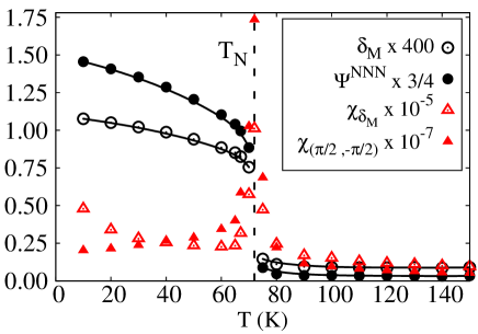
Figure 3: (color online) Filled (open) circles indicate the bicollinear AFM order parameter $\Psi^{NNN}$ (the $\mathcal{M}_{\rm ono}$ lattice distortion $\delta_{M}$) at $\tilde{g}_{12}=0.24$, $\tilde{g}_{66}=0$, $J_{\rm H}=0.1$ eV, and $J_{\rm NN}=J_{\rm NNN}=0$. Magnetic and lattice susceptibilities, $\chi_{(\pi/2,-\pi/2)}$ and $\chi_{\delta_{M}}$, are also shown (filled and open triangles, respectively). $T_{\rm N}$ denotes the first-order Neél temperature.

Another important result unveiled here is that the bicollinear/$\mathcal{M}_{\rm ono}$ phase transition was found to be strongly first order, in agreement with experiments bao , as indicated by the order parameters discontinuities shown in Fig. 3 and by the MC-time evolution histogram shown in Fig. 4 (a). The reason is that at high temperature $(\pi,0)$ fluctuations first develop (as implied by the inset of Fig. 2), leading to a free energy local minimum. However, upon further cooling the bicollinear minimum with a different symmetry also develops and eventually a crossing occurs with first-order characteristics because one local state cannot evolve smoothly into the other.

Remarkably, in addition to reproducing properly the FeTe structural/magnetic transitions, the correct behavior for the resistivity anisotropy reverse1 ; reverse2 is also observed. In the $(\pi,0)$ collinear phase, FS nesting opens a pseudogap for the $yz$ orbital shuhua13 ; shuhua ; PG-our . Because this orbital relates to electronic hopping along the ferromagnetic $y$-axis, then the FM resistivity is the largest in pnictides. However, the reversed anisotropy with lower resistance along the FM direction (open circles) was found in the bicollinear phase Fig. 4 (b) (the technique used was explained in shuhua ). Moreover, we have noticed that this reversed effect is amplified as $J_{\rm H}$ increases. The key clues to explain the effect are now clear: (i) when an electron hops along the plaquette diagonal in the AFM direction it pays an energy $J_{\rm H}$, but the hopping along the plaquette diagonal FM direction does not have this penalization; (ii) because FS nesting does not involve wavevectors such as $(\pi/2,-\pi/2)$, then pseudogaps are not created due to nesting as in pnictides. Then, in essence, the reversed resistance found here is characteristic of physics of large Hund coupling materials hund-aniso , such as manganites CMR , where it is also known that the AFM direction is more resistive than the FM direction.

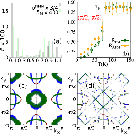
Figure 4: (color online) (a) Histogram of the MC time evolution of $\Psi^{NNN}$ and $\delta_{M}$, at the critical temperature of Fig. 3 ($T=72$ K), illustrating its bimodal character compatible with first-order characteristics. (b) Resistance ($h/2e^{2}$ units) vs. temperature in the bicollinear state ($\tilde{g}_{12}=0.24$, $\tilde{g}_{66}=0$, $J_{\rm H}=0.2$ eV, no Heisenberg terms). Filled (open) symbols denote resistivities along the AFM (FM) direction. (c,d) Symmetrized Fermi surface ($\tilde{g}_{12}=0.24$, $\tilde{g}_{66}=0$, $J_{\rm H}=0.2$ eV, no Heisenberg terms). (c) is in the high temperature paramagnetic phase ($T=360$ K); (d) is in the bicollinear phase ($T=10$ K). The FS orbital composition notation is blue ($xz$), green ($yz$), and red ($xy$). In the non-symmetrized FS (not shown) a gap opens along the AFM diagonal direction in the $xz$ and $yz$ orbitals, compatible with the resistivity results.

A paradox of FeTe is that first principles studies predict FS nesting and, thus, $(\pi,0)$ order as in pnictides. For this reason, we calculated the FS at couplings where the ground state is $\mathcal{M}_{\rm ono}$. Figure 4 (c) shows the FS in the high temperature $\mathcal{T}_{\rm etra}$ state. It is similar to that of the iron pnictides, thus suggestive of $(\pi,0)$ order upon cooling (the $\Gamma$ centered features are blurry because of how a shallow pocket is affected by temperature). However, as shown before, because of the sharp first-order transition the $\mathcal{M}_{\rm ono}$ state reached at low temperature has a peculiar FS [Fig. 4 (d)]: while the electron pockets are similar, the squarish $\Gamma$ hole pocket is different from that of pnictides. In addition “shadow bands” features at $(\pm\pi/2,\pm\pi/2)$ develop, as observed in ARPES xia , indicative of couplings stronger than for pnictides.

Discussion. Using computational techniques applied to the spin-fermion model including a spin-lattice $\mathcal{M}_{\rm ono}$ distortion in the $B_{\rm 2g}$ channel, we show that the (often puzzling) phenomenology of FeTe can be well reproduced. This includes the presence of bicollinear magnetic order and $\mathcal{M}_{\rm ono}$ lattice distortions, a strong first-order $\mathcal{T}_{\rm etra}$-$\mathcal{M}_{\rm ono}$ transition, Fermi surfaces at high temperature that naively would favor $(\pi,0)$ magnetic order, and last but not least also the low-temperature reversed anisotropic resistances between the AFM and FM directions. Moreover, all this is achieved with spin-lattice dimensionless couplings substantially less than 1, and with associated lattice distortions $\delta_{M}\sim 10^{-3}$ as in FeTe experiments.

While in pnictides the resistance anisotropy is related to FS nesting and a pseudogap in the $yz$ orbital PG-our , here we argue that in chalcogenides the strength of the Hund coupling is more important for transport since the reversed anisotropy increases with $J_{\rm H}$. To our knowledge, the spin-lattice interaction discussed here provides the first physical explanation of a vast array of experimental challenging results in FeTe.

Acknowledgments. Discussions with S. Liang, P. Dai, and J. Tranquada are acknowledged. C.B. was supported by the National Science Foundation, under Grant No. DMR-1404375. E.D. and A.M. were supported by the US Department of Energy, Office of Basic Energy Sciences, Materials Sciences and Engineering Division.

SUPPLEMENTAL
MATERIAL

In this supplemental section, technical details and additional results are provided.

S1 LATTICE DISPLACEMENTS

The lattice variables $\delta_{\bf i,\nu}=(\delta^{x}_{\bf i,\nu},\delta^{y}_{\bf i,\nu})$, with $\nu$ ranging from 1 to 4, that enter in the definition of $\epsilon_{66}$ and $\epsilon_{12}$, the orthorhombic and monoclinic lattice distortions respectively, represent the distance between an Fe atom at site ${\bf i}$ (filled circles in Fig. S1) and one of its four neighboring As or Te atoms (open circles in the figure and labeled by the index $\nu$). The As/Te atoms are allowed to move locally from their equilibrium position, but only along the directions $x$ and $y$ (the $z$ coordinate does not participate in the planar lattice distortions addressed here).

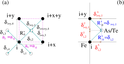
Figure S1: (color online) (a) Schematic representation of the equilibrium position of the Fe-Te/As lattice (projected on the $x$-$y$ plane). Four Fe atoms are indicated with filled circles and labeled by their site index ${\bf i}$. The open circles indicate the projection of the equilibrium position of the As/Te atoms on the $x$-$y$ plane. The distance between an Fe atom at site ${\bf i}$ and its four neighboring As/Te atoms is indicated by $\delta_{{\bf i},\nu}$ with $\nu$ running from 1 to 4 (turquoise arrows). In equilibrium $\delta_{{\bf i},\nu}=\sqrt{2}a_{0}/2$. The dashed lines indicate $a_{x}=a_{y}=a_{0}$, the equilibrium distance between neighboring irons. (b) Sketch representing the variables $\delta_{{\bf i},\nu}^{x}$ and $\delta_{{\bf i},\nu}^{y}$ (brown arrows) for labels (${\bf i},2$) and (${\bf i+y},1$) in the equilibrium configuration. For an illustration of the non-equilibrium $\delta_{{\bf i},\nu}$ see shuhua13 .

S2 METHODS

The Hamiltonian $H_{\rm SF}$ defined in the main text was studied using a Monte Carlo method shuhua ; CMR applied to (i) the localized spin degrees of freedom ${\bf S_{i}}$ assumed classical, (ii) the atomic displacements $(\delta^{x}_{{\bf i},\nu},\delta^{y}_{{\bf i},\nu})$ that determine the local orthorhombic or monoclinic lattice distortions $\epsilon_{66}({\bf i})$ shuhua13 ; chris and $\epsilon_{12}({\bf i})$, (iii) the global orthorhombic distortion $(r_{x},r_{y})$, and (iv) the global monoclinic distortion $\theta$. As already explained, in the MC simulation the As/Te atoms are allowed to move from their equilibrium positions on the $x-y$ plane but the Fe atoms can only move globally in two ways: (i) via a global orthorhombic distortion characterized by a global displacement $(r_{x},r_{y})$ from the equilibrium position $(x^{(0)}_{i},y^{(0)}_{i})$ of each Fe atom, with $r_{\alpha}=1+\Delta_{\alpha}$ ($\Delta_{\alpha}\ll 1$) and $\alpha=x$ or $y$ [see panel (c) of Fig. 1, main text]; (ii) via the angle between two orthogonal Fe-Fe bonds which is allowed to change globally to $90^{o}+\theta$ with the four angles in the monoclinic plaquette adding to $360^{o}$ so that the following angle in the plaquette becomes $90^{o}-\theta$, with $\theta$ a small angle [see panel (d) of Fig. 1, main text]. After the global distortion the new position of the Fe atom is given by

$$\biggl{\{}\begin{array}[]{ll}x_{i}=x^{(0)}_{i}r_{x}\cos\theta-y^{(0)}_{i}r_{y}\sin\theta\\ y_{i}=-x^{(0)}_{i}r_{x}\sin\theta+y^{(0)}_{i}r_{y}\cos\theta.\end{array}$$ (S1)

When an orthorhombic distortion is stabilized, the variables $\delta^{s}_{\bf i,\nu}$ satisfy the constrain

$$2Na_{s}=\sum_{{\bf i}=1}^{N}\sum_{\nu=1}^{4}|\delta^{s}_{\bf i,\nu}|,$$ (S2)

where $N$ is the number of Fe sites, $s=x,y$, and $a_{s}=a_{0}r_{s}$ is the constant Fe-Fe distance along the $s$ direction which is equal to $a_{0}$ in the undistorted tetragonal phase as shown in panel (c) of Fig. 1 (main text). The orthorhombic distortion order parameter $\delta_{O}$ is then given by

$$\delta_{O}={|a_{x}-a_{y}|\over{a_{x}+a_{y}}}={a_{0}|r_{x}-r_{y}|\over{a_{0}(r_{x}+r_{y})}}.$$ (S3)

Since $r_{s}=1+\Delta_{s}$ and $s=x$, $y$, then

$$\delta_{O}={|1+\Delta_{x}-(1+\Delta_{y})|\over{1+\Delta_{x}+1+\Delta_{y}}}\approx{1\over{2}}{|\Delta_{x}-\Delta_{y}|}.$$ (S4)

On the other hand, when a monoclinic distortion is stabilized the constraint satisfied by $\delta^{s}_{\bf i,\nu}$ is given by

$$2Nd_{x+y}=\sum_{{\bf i}=1}^{N}(|\delta_{{\bf i},4}|+|\delta_{{\bf i},2}|),$$ (S5)

and

$$2Nd_{x-y}=\sum_{{\bf i}=1}^{N}(|\delta_{{\bf i},3}|+|\delta_{{\bf i},1}|),$$ (S6)

where $d_{\mu}$ is the length of the plaquette’s diagonal along the $\mu$ direction of the plaquette formed by four Fe atoms. In the tetragonal phase $d_{\mu}=\sqrt{2}a_{0}$ while in the monoclinic phase $d_{\mu}=\sqrt{2}a_{0}\sqrt{1-\cos(90^{o}\pm\theta)}$ with the plus (minus) sign for $\mu=x-y$ ($x+y$) [see panel (d) of Fig. 1, main text]. The monoclinic distortion order parameter $\delta_{M}$ is then given by

$$\delta_{M}={|d_{x+y}-d_{x-y}|\over{d_{x+y}+d_{x-y}}}=\\ {\sqrt{2}a_{0}|(1-\sin\theta)^{1/2}-(1+\sin\theta)^{1/2}|\over{\sqrt{2}a_{0}((1-\sin\theta)^{1/2}+(1+\sin\theta)^{1/2})}}\approx{\theta\over{2}}.$$ (S7)

In summary, Monte Carlo simulations are performed on the values for the lattice variables $r_{x}$, $r_{y}$, $\theta$, and $\delta^{s}_{{\bf i},\nu}$, and also on the localized spin variables ${\bf S_{i}}$.

For each fixed Monte Carlo configuration of spins, atomic positions and global distortions, the remaining quantum fermionic Hamiltonian is diagonalized. The simulations were performed varying the temperature $T$ and the spin-lattice dimensionless couplings $\tilde{g}_{66}$ and $\tilde{g}_{12}$. The latter are defined by $\tilde{g}_{66}={2g_{66}\over{\sqrt{kW}}}$ and $\tilde{g}_{12}={2g_{12}\over{\sqrt{kW}}}$ where $W=3$ eV is the bandwidth of the tight-binding portion of the Hamiltonian and $k$ is a constant that appears in $H_{\rm Stiff}$ (for details see shuhua13 ). The range of values explored for these dimensionless coupling constants was chosen so that the orthorhombic and monoclinic distortions (also dimensionless defined) agree with the experimental values that range from 0.003 to 0.007 bao ; li ; huang .

The fermionic exact diagonalization technique results can be obtained comfortably only on up to $8\times 8$ lattices which is the cluster size used in this work. However, twisted boundary conditions were also used salafranca in the evaluation of the resistivities and Fermi surfaces (FS), effectively increasing the lattice size as explained in early efforts shuhua13 . Most couplings were fixed to values used successfully in previous investigations shuhua for simplicity: ${J_{\rm H}}$=$0.1$ eV, ${J_{\rm NN}}$=$0.012$ eV, and ${J_{\rm NNN}}$=$0.008$ eV. However, results for ${J_{\rm H}}$=$0.2$ eV and ${J_{\rm NN}}$=${J_{\rm NNN}}$=0 were also discussed in the main text.

In the Monte Carlo simulations typically 5,000 MC lattice sweeps were used for thermalization and 10,000 to 25,000 for measurements, at each temperature and parameter values investigated. In addition to the $B_{\rm 2g}$ order parameter, the magnetic transition was also determined from the behavior of the magnetic susceptibility defined as

$$\chi_{S(k_{x},k_{y})}=N\beta\langle S(k_{x},k_{y})-\langle S(k_{x},k_{y})\rangle\rangle^{2},$$ (S8)

where $\beta=1/k_{B}T$, $N$ is the number of lattice sites, and $S(k_{x},k_{y})$ is the magnetic structure factor at wavevector $(k_{x},k_{y})$ obtained via the Fourier transform of the real-space spin-spin correlations measured in the MC simulations. To study the collinear [bicollinear] AFM state $(k_{x},k_{y})$ was set to $(\pi,0)$ [$(\pi/2,-\pi/2)$].

Besides the lattice order parameter $\delta_{O}$ given in Eq. S3, the orthorhombic structural transition was determined from the behavior of the lattice susceptibility defined as

$$\chi_{\delta_{O}}=N\beta\langle\delta_{O}-\langle\delta_{O}\rangle\rangle^{2}.$$ (S9)

Reciprocally, the monoclinicic structural transition was studied via its order parameter, i.e. the monoclinic distortion $\delta_{M}$ given in Eq. S7, and also through the lattice susceptibility defined as

$$\chi_{\delta_{M}}=N\beta\langle\delta_{M}-\langle\delta_{M}\rangle\rangle^{2}.$$ (S10)

S3 ADDITIONAL PHASE DIAGRAMS

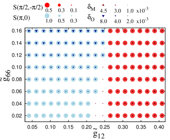
Figure S2: (color online) Phase diagram at $T=10$ K of the spin fermion model, including Heisenberg couplings with the values indicated in the Methods Section, varying the dimensionless couplings to the orthorhombic and monoclinic distortions. The size of the blue (red) circles is proportional to the strength of the collinear (bicollinear) AFM order. The size of the bottom side up (down) triangles is proportional to the magnitude of the orthorhombic (monoclinic) distortion. The actual scales used are shown at the top of the figure.

The phase diagram as a function of the couplings $\tilde{g}_{66}$ and $\tilde{g}_{12}$ at $T=10$ K is presented in Fig. S2 including Heisenberg couplings. It is important to remember that in the absence of spin-lattice couplings the SF model already develops a collinear AFM ground state due to the comparable NN and NNN hoppings in the tight-binding term of the Hamiltonian (and the concomitant NN and NNN Heisenberg interactions between the localized spins if included shuhua ). The coupling $\tilde{g}_{66}$ that couples the short-range $B_{\rm 1g}$ magnetic nematic operator to the orthorhombic distortion stabilizes a small orthorhombic distortion that increases monotonically with the value of this spin-lattice coupling, as indicated by the size of the inverted triangles in the figure. The blue circles indicate the concomitant presence of collinear $(\pi,0)$ AFM order. The figure shows that, regardless of $\tilde{g}_{66}$, the coupling $\tilde{g}_{12}$, between the monoclinic lattice distortion and the $B_{\rm 2g}$ magnetic nematic operator, has to reach a finite value close to 0.25 to stabilize the bicollinear AFM state indicated by the red circles in the figure. The bicollinear magnetic order is accompanied by a monoclinic lattice distortion indicated by the triangles whose size increases monotonically with $\tilde{g}_{12}$.

It is interesting to observe that there is a region in the phase diagram Fig. S2 where the monoclinic distortion is stabilized, but the magnetic order is neither collinear nor bicollinear. This is caused by the competition between $\tilde{g}_{12}$, that after inducing the monoclinic distortion induces the bicollinear magnetic order, and the NN and NNN Heisenberg couplings that favor a collinear $(\pi,0)$ magnetic state. Thus, $\tilde{g}_{12}$ is able to induce the lattice distortion before it clearly stabilizes the bicollinear magnetic order. The fact that the value of $\tilde{g}_{12}$ that stabilizes the bicollinear state is larger than the value of $\tilde{g}_{66}$ needed to obtain the experimentally observed magnitude of the orthorhombic distortion is also a result of the effect of the Heisenberg terms in the Hamiltonian that favor the collinear AFM state.

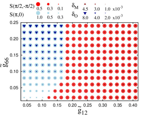
Figure S3: (color online) Phase diagram at $T=10$ K corresponding to the spin-fermion model for the case $J_{\rm NNN}$=$J_{\rm NN}$=0, varying the spin-lattice couplings that lead to the orthorhombic and monoclinic distortions. The size of the blue (red) circles is proportional to the strength of the collinear (bicollinear) AFM order, while the size of the bottom side up (down) triangles is proportional to the magnitude of the orthorhombic (monoclinic) distortion.

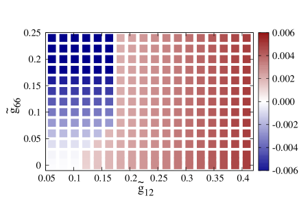
Figure S4: (color online) Orthorhombic, $\delta_{O}$ (blue), and monoclinic, $\delta_{M}$ (red), lattice distortions varying $\tilde{g}_{66}$ and $\tilde{g}_{12}$ at $T=10$ K using the spin-fermion model with $J_{\rm NNN}$=$J_{\rm NN}$=0. The scale on the right shows that the lattice distortions obtained numerically are within the correct order of magnitude when compared with experimental data bao ; li ; huang . The values for the orthorhombic distortion are plotted with a negative sign for simplicity to display.

In Fig. S3 we display the low-temperature phase diagram in the plane $\tilde{g}_{12}-\tilde{g}_{66}$ for the case $J_{\rm NN}$=$J_{\rm NNN}$=0. Again the collinear and bicollinear phases are stabilized but, as expected, smaller values of the monoclinic coupling are needed to induce the monoclinic phase. Note, however, that a finite value $\tilde{g}_{12}\approx 0.1$ is still required to stabilize the bicollinear phase because the tight-binding term in the Hamiltonian still favors a collinear magnetic state via FS nesting.

The strength of the lattice distortion of Fig. S3 is shown in Fig. S4. A reasonable coupling $\tilde{g}_{66}\approx 0.2$ is needed to reproduce the experimental value of the orthorhombic distortion corresponding to the 122 parent compounds. The scale shows that the range in the values of the stabilized monoclinic distortion is also in qualitative agreement with experiments bao ; li ; huang .

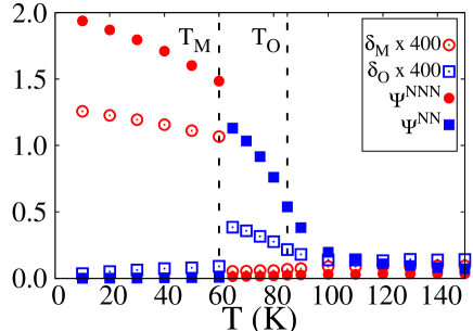
Figure S5: (color online) Orthorhombic, $\delta_{O}$ (blue open squares), and monoclinic, $\delta_{M}$ (red open circles), lattice distortions and the spin nematic order parameters $\Psi^{NN}$ (blue filled squares) and $\Psi^{NNN}$ (red filled circles) as a function of temperature corresponding to the case $\tilde{g}_{12}=0.29$, $\tilde{g}_{66}=0.05$ and with the inclusion of Heisenberg couplings.

S4 UNEXPECTED INTERMEDIATE TEMPERATURE RANGE

When Heisenberg couplings are included, the inset of Fig. 2 (main text) shows an exotic region where the bicollinear/monoclinic transition is preceded by an orthorhombic transition upon cooling. In Fig. S5 we show the magnetic and structural order parameters for both types of transitions in this unexpected regime. The transition to the collinear/orthorhombic region occurs at about $T=80$ K and it appears to be continuous, while the bicollinear/monoclinic transition occurs at $T=60$ K and is strongly first order. Note that in our simulations the orthorhombic phase appears to be accompanied by a collinear magnetic state while experimentally the orthorhombic phase that precedes the monoclinic state in FeTe with excess Fe is magnetically incommensurate mizuguchi ; rodriguez . We may need either larger lattices or the explicit addition of extra irons in order to capture the magnetic incommensurability of this phase.

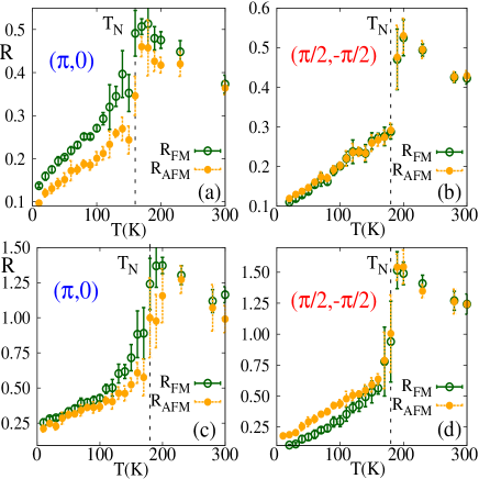
Figure S6: (color online) Resistance ($h/2e^{2}$ units) vs. temperature along the AFM (orange points) and FM (green points) directions in: (a) the collinear/orthorhombic state at $\tilde{g}_{66}=0.16$, $\tilde{g}_{12}=0.00$, $J_{\rm H}=0.10$ eV, and nonzero Heisenberg couplings; (b) same as (a) but for the bicollinear/monoclinic state with $\tilde{g}_{66}=0$ and $\tilde{g}_{12}=0.40$; (c) same as (a) but for $J_{\rm H}=0.20$ eV; (d) same as (b) but for $J_{\rm H}=0.20$ eV.

S5 REVERSED RESISTIVITY

A very interesting result that is reproduced by our study is the anisotropy observed in the planar resistivity of FeTe.

In general, one of the most puzzling behaviors observed in the Fe-based materials is the anisotropic behavior of the in-plane resistivity as the temperature decreases. In the pnictides the cause of the anisotropy is usually attributed to nematicity of electronic origin. In isovalent or electron doped pnictides the resistivity anisotropy develops in the orthorhombic phase and the resistivity is lower along the direction with the largest lattice constant which becomes the antiferromagnetic direction below the magnetic critical temperature. This behavior is in principle counterintuitive because in the colossal magnetoresistive manganites it is well-known that electrons move better in ferromagnetic states. In principle this is not the case in the pnictides due to the geometry of the orbitals that appear at the Fermi surface. Interestingly, a “reversed” or “negative” anisotropy in the resistivity has been observed in the chalcogenides, both in the parent compound FeTe uchida ; jiang and also in FeSe tanatar .

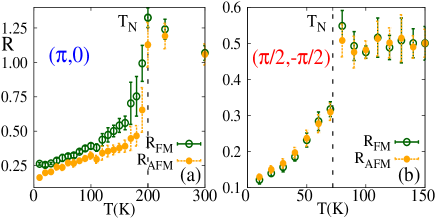
Figure S7: (color online) Resistance vs. temperature along the AFM (orange points) and FM (green points) directions in: (a) the collinear/orthorhombic state for $\tilde{g}_{66}=0.24$, $\tilde{g}_{12}=0.00$, $J_{\rm H}=0.20$ eV, and $J_{\rm NNN}$=$J_{\rm NN}$=0; (b) same as (a) but for the bicollinear/monoclinic state with $\tilde{g}_{66}=0.00$, $\tilde{g}_{12}=0.24$, $J_{\rm H}=0.10$ eV, and $J_{\rm NNN}$=$J_{\rm NN}$=0.

The resistance $R$ along the AFM and FM directions was calculated as a function of the temperature following the procedure described in shuhua implementing twisted boundary conditions so that the number of accessible momenta along the $x$ and $y$ directions was as large as $L=256$. In Fig. S6 (a) we show the planar resistance in the collinear/orthorhombic phase corresponding to $\tilde{g}_{66}=0.16$, $\tilde{g}_{12}=0.00$, $J_{\rm H}=0.10$ eV, and nonzero Heisenberg couplings. In this case, the resistance is the smallest along the AFM direction ($x$-direction in the square lattice) in agreement with previous theoretical investigations shuhua13 and with the experimental data for pnictides fisher.science1 . In the bicollinear phase, obtained for example at $\tilde{g}_{66}=0$ and $\tilde{g}_{12}=0.40$ we actually observe the reversed behavior as shown in Fig. S6 (b) although here the anisotropy is very small aniso . However, it is experimentally known that the magnetic moment measured in the chalcogenides is larger than the one in the pnictides bao ; li and, for this reason, we have repeated the simulation increasing the Hund coupling from 0.10 eV to 0.20 eV. As it can be observed in Fig. S6 (d) the reversed anisotropy effect is now enhanced. On the other hand, a similar increase in Hund coupling decreases the resistance anisotropy in the orthorhombic phase as shown in panel (c) of the same figure. These results indicate that the reversed anisotropy is favored (hindered) by the increase (decrease) in the magnitude of the magnetic moments. A similar response to the Hund coupling is observed for the case where the Heisenberg couplings are zero, as presented in the main text: in Fig.  S7 we display the results illustrating how the anisotropy is reduced with increasing Hund coupling in the collinear phase (panel a) while the reversed anisotropy decreases when the Hund coupling is reduced in the bicollinear phase (panel b).

As already explained in the main text, we believe that this “reversed” anisotropy occurs for reasons similar to those unveiled in manganite investigations CMR , namely when electrons move along the AFM direction they must pay an energy as large as $J_{\rm H}$, while along the FM direction there is no such penalization. This is compatible with the observation that the magnitude of the reversed effect increases with $J_{\rm H}$.

References

- (1) D. C. Johnston, Adv. Phys. 59, 803 (2010).
- (2) P. C. Dai, J. P. Hu, and E. Dagotto, Nature Phys. 8, 709 (2012).
- (3) Y. Zhang, F. Chen, C. He, L.X. Yang, B.P. Xie,Y.L. Xie, X.H. Chen, M. Fang, M. Arita, K. Shimada,H. Namatame, M. Taniguchi, J.P. Hu,D. L. Feng , Phys. Rev. B 82, 165113 (2010).
- (4) Y. M. Dai, A. Akrap, J. Schneeloch, R. D. Zhong, T. S. Liu, G. D. Gu, Q. Li, and C. C. Homes, Phys. Rev. B 90, 121114(R) (2014).
- (5) Y. Xia,D. Qian,L. Wray,D. Hsieh,G.F. Chen,J.L. Luo,N.L. Wang,M.Z. Hasan, Phys. Rev. Lett. 103, 037002 (2009).
- (6) P.-H. Lin, Y. Texier, A. Taleb-Ibrahimi, P. Le Fevre, F. Bertran, E. Giannini, M. Grioni, and V. Brouet, Phys. Rev. Lett. 111, 217002 (2013).
- (7) W. Bao,Y. Qiu, Q. Huang, M.A. Green, P. Zajdel, M.R. Fitzsimmons, M. Zhernenkov, S. Chang, M. Fang, B. Qian, E.K. Vehstedt, J. Yang, H.M. Pham,L. Spinu, Z.Q. Mao Phys. Rev. Lett. 102, 247001 (2009); S. Li ,C. delaCruz,Q. Huang,Y. Chen,J.W. Lynn,J. Hu,Y.L. Huang,F.C. Hsu,K.W. Yeh,M.K. Wu, P. Dai , Phys. Rev. B 79, 054503 (2009).
- (8) E. Dagotto, T. Hotta, and A. Moreo, Phys. Rep. 344, 1 (2001).
- (9) F. Ma, W. Ji, J. Hu, Z.-Y. Lu, and T. Xiang, Phys. Rev. Lett. 102, 177003 (2009).
- (10) C. Fang, B. Andrei Bernevig, and J. Hu, EPL, 86, 67005 (2009).
- (11) In addition, discrepancies with neutron scattering have been unveiled: O.J. Lipscombe,G.F. Chen,C. Fang,T.G. Perring,D.L. Abernathy,A.D. Christianson,T. Egami,N. Wang,J. Hu, P. Dai, Phys. Rev. Lett. 106, 057004 (2011); S. Chi,J.A. Rodriguez-Rivera,J.W. Lynn,C. Zhang,D. Phelan,D.K. Singh,R. Paul,P. Dai, Phys. Rev. B 84, 214407 (2011).
- (12) Hartree-Fock real-space studies of the five orbital Hubbard model without lattice distortions revealed a rich phase diagram when varying and the electronic density (see Q. Luo and E. Dagotto, Phys. Rev. B 89, 045115 (2014)). Among the plethora of different magnetic states, the E phase was found but in a very small and unrealistic region at large and .
- (13) G. F. Chen, Z. G. Chen, J. Dong, W. Z. Hu, G. Li, X. D. Zhang, P. Zheng, J. L. Luo, and N. L. Wang, Phys. Rev. B 79, 140509(R) (2009).
- (14) D. Fobes,I.A. Zaliznyak,Z.Xu,R. Zhong, G. Gu, J.M.Tranquada,L. Harriger,D. Singh,V.O. Garlea,M. Lumsden,B. Winn, , Phys. Rev. Lett. 112, 187202 (2014).
- (15) Q. Huang, Y. Qiu, Wei Bao, M. A. Green, J. W. Lynn, Y. C. Gasparovic, T. Wu, G. Wu, and X. H. Chen, Phys. Rev. Lett. 101, 257003 (2008).
- (16) L. Liu, et al., Phys. Rev. B 91, 134502 (2015).
- (17) J. Jiang,C. He,Y. Zhang,M. Xu,Q.Q. Ge,Z.R. Ye,F. Chen,B.P. Xie,D.L. Feng, Phys. Rev. B 88, 115130 (2013).
- (18) See, e.g., discussion and citations in intro .
- (19) I. A. Zaliznyak, Z. Xu, J. M. Tranquada, G. Gu, A. M. Tsvelik, and M. B. Stone, Phys. Rev. Lett. 107, 216403 (2011).
- (20) Other ARPES results were interpreted in terms of polarons, as in manganites, also concluding that the lattice plays an important role: Z. K. Liu et al., Phys. Rev. Lett. 110, 037003 (2013). Mechanisms that rely on Jahn-Teller distortions, double exchange processes and its associated Hund coupling, similar to those in manganites, have also been discussed theoretically (see A. M. Turner, F. Wang, and A. Vishwanath, Phys. Rev. B 80, 224504 (2009); M. Hirayama, T. Misawa, T. Miyake, and M. Imada, J. Phys. Soc. Jpn. 84, 093703 (2015)).
- (21) W.-G. Yin, C.-C. Lee, and W. Ku, Phys. Rev. Lett. 105, 107004 (2010).
- (22) S. Liang, G. Alvarez, C. Sen, A. Moreo, and E. Dagotto, Phys. Rev. Lett. 109, 047001 (2012).
- (23) S. Liang, A. Moreo, and E. Dagotto, Phys. Rev. Lett. 111, 047004 (2013).
- (24) S. Liang, A. Mukherjee, N. D. Patel, C. B. Bishop, Elbio Dagotto, and Adriana Moreo, Phys. Rev. B 90, 184507 (2014).
- (25) M. Daghofer, A. Nicholson, A. Moreo, and E. Dagotto, Phys. Rev. B 81, 014511 (2010).
- (26) The magnitude of the localized spins is set to since the actual value can be absorbed into the Hamiltonian parameters.
- (27) Note that a complete study of the bicollinear magnetic state would require a five-orbital Hubbard model with repulsion and Hund coupling , plus the lattice, all at finite temperature. Such a formidable many-body challenge is not practical, thus the SF model provides a simplification that allows for the study of structural, orbital, and magnetic effects simultaneously.
- (28) R. M. Fernandes, A. V. Chubukov, J. Knolle, I. Eremin, and J. Schmalian, Phys. Rev. B 85, 024534 (2012).
- (29) R. M. Fernandes and J. Schmalian, Supercond. Sci. Technol. 25, 084005 (2012).
- (30) The spin in and is only the localized spin for computational simplicity.
- (31) See Supplemental Material at http://link.aps.org/supplemental/…
- (32) H.-H. Kuo, J.-H. Chu, S. A. Kivelson, and I. R. Fisher, arXiv:1503.00402.
- (33) There are two degenerate bicollinear states with momentum and whose degeneracy is broken by the distortion. In this work we present results for the case in which the state with momentum is stabilized.
- (34) Y. Mizuguchi et al., Solid State Comm. 152 1047 (2012).
- (35) The low-temperature (10 K) phase diagrams varying and are also in the Suppl. Sec. SuSe [see Fig. S2 (S3) with (without) Heisenberg couplings]: in a broad range of couplings the bicollinear/ state is indeed spontaneously stabilized.
- (36) E.E. Rodriguez,C. Stock,P. Zajdel,K.L. Krycka, C.F. Majkrzak,P. Zavalij,M.A. Green, Phys. Rev. B 84, 064403 (2011).
- (37) M. Daghofer, Q.-L. Luo, R. Yu, D. X. Yao, A. Moreo, and E. Dagotto, Phys. Rev. B 81, 180514(R) (2010).
- (38) Chalcogenides have higher magnetic moments than pnictides, thus likely larger Hund couplings. We also noticed that for eV we found that the reversed anisotropy was still there but smaller (see Suppl. Sec. SuSe ).

References

- (1) S. Liang, A. Moreo, and E. Dagotto, Phys. Rev. Lett. 111, 047004 (2013).
- (2) E. Dagotto, T. Hotta, and A. Moreo, Phys. Rep. 344, 1 (2001).
- (3) S. Liang, G. Alvarez, C. Sen, A. Moreo, and E. Dagotto, Phys. Rev. Lett. 109, 047001 (2012).
- (4) S. Liang, A. Mukherjee, N. D. Patel, C. B. Bishop, E. Dagotto, and A. Moreo, Phys. Rev. B 90, 184507 (2014).
- (5) W. Bao et al., Phys. Rev. Lett. 102, 247001 (2009).
- (6) S.L. Li et al., Phys. Rev. B 79, 054503 (2009).
- (7) Q. Huang, Y. Qiu, Wei Bao, M. A. Green, J. W. Lynn, Y. C. Gasparovic, T. Wu, G. Wu, and X. H. Chen, Phys. Rev. Lett. 101, 257003 (2008).
- (8) J. Salafranca, G. Alvarez, and E. Dagotto, Phys. Rev. B 80, 155133 (2009).
- (9) Y. Mizuguchi et al., Solid State Comm. 152, 1047 (2012).
- (10) E. E. Rodriguez et al., Phys. Rev. B 84, 064403 (2011).
- (11) L. Liu, T. Mikami, M. Takahashi, S. Ishida, T. Kakeshita, K. Okazaki, A. Fujimori, and S. Uchida, Phys. Rev. B 91, 134502 (2015).
- (12) J. Jiang et al., Phys. Rev. B 88, 115130 (2013).
- (13) M. A. Tanatar et al., arViv: 1511.04757.
- (14) J-H. Chu, J. G. Analytis, K. De Greve, P. L. McMahon, Z. Islam, Y. Yamamoto, and I. R. Fisher, Science 329, 824 (2010).
- (15) Notice that in the bicollinear phase illustrated in Fig. 1 of the main text, the AFM direction is .