Sequential Principal Curves Analysis

Abstract

This report includes all the technical details of the Sequential Principal Curves Analysis (SPCA) in a single document. SPCA is an unsupervised nonlinear and invertible feature extraction technique. The identified curvilinear features can be interpreted as a set of nonlinear sensors: the response of each sensor is the projection onto the corresponding feature. Moreover, it can be easily tuned for different optimization criteria –e.g. infomax, error minimization, decorrelation– by choosing the right way to measure distances along each curvilinear feature.

Even though proposed in [1] and shown to work in multiple modalities in [2], the SPCA framework has its original roots in the nonlinear ICA algorithm in [3]. Later on, the SPCA philosophy for nonlinear generalization of PCA originated substantially faster alternatives at the cost of introducing different constraints in the model. Namely, the Principal Polynomial Analysis (PPA) [4], and the Dimensionality Reduction via Regression (DRR) [5]. This report illustrates the reasons why we developed such family and is the appropriate technical companion for the missing details in [1, 2]. See also the data, code and examples in the dedicated sites http://isp.uv.es/spca.html and http://isp.uv.es/after_effects.html

I Introduction

Classical unsupervised learning such as Principal Components Analysis (PCA) and Independent Component Analysis (ICA) is useful to design artificial sensory systems and to understand the organization of natural sensory systems. On the artificial side, examples include representations/transforms for image coding [6, 7, 8, 9] and image categorization [10, 11]. On the natural side, examples include the analysis of visual cortex [12, 13, 14, 15, 16]. PCA and ICA obtain basis of the space according to different optimization criteria. These basis functions can be interpreted as linear sensors: the projection of data onto these basis represents the response of the set of sensors. PCA defines a sensor hierarchy: for example, an image sensory system made out of principal directions with highest eigenvalues minimizes the image reconstruction error [6, 7]. In ICA, the basis is intended to provide responses as independent as possible, which is equivalent to design a sensory system that maximizes the transmitted information (infomax) [17, 18].

Even though linear unsupervised techniques have been successful to (1) design sets of artificial sensors, and (2) to explain the receptive fields of biological sensors, they have fundamental problems:

• Sensors are linear. Linear transforms are not efficient when the data do not come from a linear manifold or when the natural sensory system at hand is nonlinear. For example, in vision, PCA or ICA models are too simple for natural images [19, 20, 21, 22, 3, 23, 24, 25, 26], and linear feature extraction cannot explain the nonlinear responses of spatial frequency analyzers in V1 [27, 28, 29, 30, 31].

• Features are treated independently. Projecting the data in each basis function independently is an advantage to interpret each dimension of the transform as a separate sensor. However, this simplistic model ignores eventual relations between linear responses. For instance, in vision, contrast masking experiments [27, 28] and neuron recordings [29, 30, 31] indicate inhibitory interactions between linear mechanisms. Moreover, coefficients of linear ICA-like image transforms are not independent [19, 20, 21, 23, 3, 24, 25, 26, 22].

• The metric is global. Linear transforms imply a constant Jacobian and hence the induced metric is global, i.e. equal in each point [32, 22, 33]. This is an important restriction since artificial and natural sensory systems have limited resolution and more resources have to be allocated in more populated regions of the space. This means a point-dependent resolution/metric/sensitivity, and not just a different weight per dimension [28, 33].

A number of nonlinear manifold learning techniques have been developed that could be used to address the obvious problems of linear techniques. Unfortunately, more sophisticated methods are harder to interpret as a set of sensors. In order to be suitable for the interpretation or design of sensory systems, a nonlinear technique should have the following features:

• Explicit form of the sensors. An explicit representation of the sensors (analogous to the principal directions in PCA or the independent directions in linear ICA) is desirable. Implicit transforms may be flexible enough to capture data nonlinearities but one has no separate access to the properties of each sensor, which is mandatory if the properties of specific biological sensors have to be reproduced. Note that an explicit set of nonlinear sensors in the input space is helpful since it defines a curvilinear coordinate system. In this situation the response of such sensory system is just an intuitive change of coordinates.

• Out-of-sample problem. It is important that the method is applicable to data which is not in the training set.

• Invertibility. Invertibility ensures that changes in the response domain may be analyzed back in the original space. This is useful to assess the representation error when considering a reduced set of sensors (dimensionality reduction) or when they have limited resolution (transform quantization). Invertibility is also useful to obtain the meaning of the coordinates of the transform domain back in the input space.

• Tunable metric. As stated above, sensitivity should be focused on specific regions of the input space according to the Probability Density Function (PDF). The method has to include different principles guiding this point-dependent metric. A clear definition of the metric according to different organization criteria allows to explore the principles underlying the behavior of biological systems.

Conventional nonlinear manifold learning methods do not fulfill all the above requirements at the same time.

For instance, though efficient in many tasks, spectral methods [34, 35, 36] and kernel methods [37] do not generally yield intuitive mappings between the original and the intrinsic curvilinear coordinates of the low dimensional manifold. In addition, even though a metric can be derived from particular kernel functions [38], the interpretation of the transformation is hidden behind implicit mappings, and out-of-sample extensions are typically difficult, if not impossible.

An alternative family of manifold learning methods describe complicated manifolds as a mixture of local models [39] that may be merged into a single global representation [40, 41, 42, 43]. The explicit direct and inverse transforms can be derived from the obtained mixture model. However, explicit description of the sensors is not straightforward, and moreover, the effect of the local coordination in the (eventually point-dependent) metric was not explicitly analyzed. In the context of nonlinear ICA, an alternative way of merging locally disconnected representations was proposed in [3]. In that case, the global representation was based on the fact that the Jacobian of the global nonlinear ICA may be differentially approximated by local linear ICA [44]. Accordingly, the global representation was obtained by integrating the Jacobian. However, obtaining the global representation through integration in arbitrary paths requires special symmetries in the manifold (e.g. Stokes condition). Moreover, the invertibility of the transform was not addressed therein [3].

Self-Organizing Maps (SOM) [45] and variants [46] are based on tuning a predefined topology in such a way that the curved sensors and the complete lattice of discrete responses are obtained simultaneously. Therefore, training is computationally demanding in highly dimensional scenarios as is the case for visual stimuli. Moreover, the appropriate choice of the SOM lattice resolution (number of discrete perceptions per dimension) requires a priori knowledge of the sensory system one wants to model. Another candidate to describe visual sensors is isometric feature mapping (Isomap) [47]. It computes geodesic distances in the manifold obtaining an unfolded representation of the data. Nevertheless, it is not invertible and hence the explicit description of the sensors in the input space is not easy to obtain. Moreover, including different design criteria in the Isomap metric is not straightforward.

Here we present the general formulation of an alternative learning technique: the Sequential Principal Curves Analysis (SPCA). The basic SPCA idea is generalizing the explicit set of sensors of linear unsupervised learning by using a set of Principal Curves (PCs). SPCA assumes a smooth manifold made of local clusters, as the local coordination literature [40, 41, 42, 43]. However, unlike [40, 41, 42, 43], no mixture of models is computed here. On the contrary, as in [3], we integrate a suitable Jacobian intended for component independence. The distinctive features of SPCA are: (i) new PDF-based Jacobian (or metric) that can be tuned to either the infomax or the error minimization principles, (ii) using the concept of secondary PCs [48], we obtain a set of non-linear sensors made of a specific sequence of secondary curves, and (iii) straightforward out-of-sample extension and invertibility.

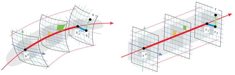
Figure 1: The SPCA leading idea is removing redundancies by unfolding the dataset along the first and secondary principal curves (PCs) while performing local equalization along the way. Left plot represents the input domain ${\bf x}$ and right plot represents the response domain ${\bf r}$. Gray regions represent the underlying PDFs. As in SOM, a curvilinear lattice is assumed (thin red, blue, and green curves). However, unlike in SOM, the computation of the whole lattice is not needed: to transform certain ${\bf x}$ just the path in bold style, made of segments of PCs, is required. Moreover, the specific resolution per dimension emerges from data: the proposed Jacobian with the embedded metric, Eq. 10, implies that highly populated regions in the input (e.g. orange area) are expanded in the response while lower density regions (e.g. green area) are shrunk. Given an origin, ${\bf x}^{o}$, in the first PC (red line) and some point of interest, ${\bf x}$, the response for the point of interest is given by the lengths (the integrals in Eq. 16) along this path: the first (or standard) PC in red, the second PC (in blue) in the orthogonal subspace at ${{\bf x}_{\bot}^{1}}$, which is the (geodesic) orthogonal projection of ${\bf x}$ on the first PC, and the third PC (in green) in the orthogonal subspace at ${{\bf x}_{\bot}^{2}}$.

Fig. 1 illustrates the SPCA concept. SPCA instrumentally requires an algorithm to draw first [49] and secondary [48] PCs from specific points (i.e. a local-to-global algorithm). Suitable choices include those in [48, 50, 51] or the one used here (see the Appendix below). However, note that the choice to draw individual PCs is not the core of SPCA, but the PDF-related metric and the specific sequential path for the Jacobian integration leading to the curvilinear coordinate system (the nonlinear sensors).

Related work includes extensions of PCA generalizing principal components from straight lines to curves, based on: (1) non-analytic principal curves [52, 53], (2) fitting analytic curves [54, 55, 56, 57], and (3) implicit methods using neural networks and autoencoders [58, 59, 60].

The distinctive property of SPCA is that it identifies an explicit system of separate sensors with tunable resolution. In [52, 53] the authors suggest that their projection method could be used for signal representation if applied sequentially. However, they acknowledge that their current setting lacks the required accuracy [53]. The nonlinear features identified by neural networks [58, 59, 60] are not explicit in the formulation, complicating their use in the interpretation of nonlinear sensors (as for instance to understand image texture analyzers in V1). Finally, the consideration of biologically plausible organization principles (such as infomax or error minimization) and their metric effects were not addressed in [52, 53, 54, 55, 56, 57, 58, 59, 60].

The work is organized as follows. Section II reviews the infomax and the error minimization principles and their geometric effects. Section III motivates the proposed Jacobian and integration path by making observations on smooth manifolds. Section IV describes our proposal: the Sequential Principal Curves Analysis with tunable metric. The experimental Section V empirically checks the SPCA assumptions and abilities through a series of examples: (1) sensible geodesic projections, (2) convergence of transform and inverse, (3) nonlinear ICA and optimal transform coding as a function of the PDF-based metric. (4) dimensionality reduction, (5) domain adaptation, (6) enhanced classification through generalization of the Mahalanobis metric. Finally the Appendix describes the instrumental algorithm used here to draw a single Principal Curve.

II Infomax, error minimization and local metric

Processing input samples ${\bf x}\in\mathbb{R}^{d}$ requires the design of an appropriate set of $d$ sensors that transform observations into ${\bf r}=R({\bf x})\in\mathbb{R}^{d}$. Limited sensor resolution or internal noise in the responses are modeled as some sort of quantization Q,

(1)

The infomax [17, 18] and error minimization [61] design principles imply different links between the sensitivity of the system (its Jacobian $\nabla R({\bf x})$), the non-Euclidean metric induced by the system [32, 22, 33], and the signal PDF, $p({\bf x})$. However, these links restrict but do not determine the response function [62, 63]. In this section we review the links and in Section III we make additional considerations that lead to a particular design for $R$.

On the one hand, infomax looks for transforms $R$ such that ${\bf r}$ has independent components or maximum entropy, which leads to [17, 18]:

$$|\nabla R({\bf x})|\propto p({\bf x})$$ (2)

On the other hand, minimization of $|{\bf x}-R^{-1}({\bf r^{\star}})|_{2}$ leads to a different constraint. The optimal MSE sensitivity fulfils [61],

$$|\nabla R({\bf x})|\propto p({\bf x})^{1/3}$$ (3)

which is consistent with the classical optimal MSE distribution of discrete perceptions in Vector Quantization [7]. The exponent accompanying the PDF in the Jacobian will be hereafter referred to as $\gamma$.

Non-linear responses have geometrical effects. Intuitively, a sensory system with non-trivial response induces a non-Euclidean metric in the input space: if the sensitivity (slope of the response) is bigger at some region of the input space, distortions in that region will be more relevant to the system. In particular, assuming that the internal representation, ${\bf r}$, is Euclidean, the following perceptual metric matrix is induced by the system at the input domain [32, 22, 33]: $M({\bf x})=\nabla R({\bf x})^{\top}\cdot\nabla R({\bf x})$.

Accordingly, relations between the sensitivity of the system and the PDF of the input space (as required by infomax or error minimization) will also give rise to relations between the induced metric and the PDF:

$$|M({\bf x})|\propto p({\bf x})^{2\gamma}$$ (4)

The above restrictions on $|\nabla R|$ and $|M|$ do not fully determine $R$. In fact, an infinite family of transforms is suitable for infomax [62, 63]. Next section makes additional considerations that inspire our proposal for $\nabla R$.

III Motivation in the infomax context

The following properties of curved smooth manifolds motivate the proposed Jacobian and integration path:

1. Global linear transforms, ${\bf v}=W\cdot{\bf x}$, are not appropriate for component independence in curved manifolds since the conditional mean with regard to one linear component (or direction), say $v_{1}$, is not constant in the range of $v_{1}$. This means that the conditional PDF, $p(v_{2},\ldots,v_{d}|v_{1})$, depends on $v_{1}$ and hence, the orthogonal subspace $(v_{2},\ldots,v_{d})$ statistically depends on $v_{1}$.

2. Unfolding along one PC is a sensible step towards independence since it makes equal the first moment (the mean) of the conditional PDFs along the PC. However, complete independence may require additional processing.

3. Additional processing after unfolding should make equal the higher order moments. For instance, if manifolds are approximated as mixtures of Gaussian clusters, the second moment (the covariance) along the PC can be made equal by local expansions (local metric changes) in the unfolded domain. In general, by choosing a metric proportional to the probability (Eq. 2), the conditional PDFs are uniformized. In this way, all the moments are constant along the PC.

III-A Unfolding along the PC: the cumulants perspective

Unfolding along PCs (or alignment of the clusters in the manifold) implies a step in the right (independence) direction but it is not enough since a metric change is still needed. This is easy to see by looking at the cumulant expansion of the conditional PDFs.

Unfolding along a PC with parameter, $u_{1}$, implies independence with regard to orthogonal subspaces iff it gives rise to:

$$p(u_{2},\ldots,u_{d}|u_{1})=p(u_{2},\ldots,u_{d})$$ (5)

Therefore, the cumulant generating functions of both sides of the above equation should be equal:

$$1-j\boldsymbol{\omega}^{\top}{\bf m}_{1}+\frac{1}{2}\boldsymbol{\omega}^{\top}\boldsymbol{m}_{2}\boldsymbol{\omega}-\ldots=1-j\boldsymbol{\omega}^{\top}{\bf m}^{\prime}_{1}+\frac{1}{2}\boldsymbol{\omega}^{\top}\boldsymbol{m}^{\prime}_{2}\boldsymbol{\omega}-\ldots$$ (6)

where ${\bf m}_{i}$ and ${\bf m}^{\prime}_{i}$ are the $i$th-order moments of each PDF, and $\boldsymbol{\omega}$ is the parameter of the characteristic functions. Independence holds if ${\bf m}_{i}={\bf m}^{\prime}_{i}$, $\forall i$.

One PC satisfies the parametric equation [49]:

$$f(u_{1})={\mathbb{E}}[{\bf x}|\lambda({\bf x})=u_{1}]$$ (7)

where $\lambda({\bf x})$ is the orthogonal projection of ${\bf x}$ on the curve, so $\{{\bf x}|\lambda({\bf x})=u_{1}\}$ is the orthogonal subspace at the curve point $u_{1}$. According to this, the curve passes through the average of the orthogonal subspace (the origin of the subspace in the unfolded representation):

$${\mathbb{E}}[u_{2},\ldots,u_{d}|u_{1}]={\bf 0},\forall u_{1}\Rightarrow{\mathbb{E}}[u_{2},\ldots,u_{d}]={\bf 0}$$ (8)

which means that unfolding along a PC makes the averages equal: ${\bf m}_{1}={\bf m^{\prime}}_{1}={\bf 0}$. However higher order moments (e.g. variance) may not be equal along the curve. Therefore, unfolding is good in independence terms (i.e. it helps to fulfill Eq. 6), but additional processing is needed to ensure the equality of all higher order moments. Next subsection shows an example based on Gaussian clusters where the additional processing after unfolding reduces to making the covariances equal (i.e. equalization).

III-B Equalization after unfolding

Here we explore the effect of unfolding and local equalization in multi information terms. To this end we consider an elementary curved manifold made of two different local clusters (Fig. 2), but the conclusions may be extended to more complicated manifolds made of local clusters.

By definition, the PC will go through the averages of the local clusters, i.e. the points $\mathbf{c}^{1}$ and $\mathbf{c}^{2}$ in our elementary example. A set of concatenated rotations with appropriate angles around the points along the PC, $\mathbf{u}=U(\mathbf{x})$, will eventually unfold the PDF by aligning the averages of each local cluster as well as the axes of the local models.

The change in multi-information, $\Delta I=I(\mathbf{x})-I(\mathbf{u})$, using this family of concatenated rotations, $U$, is easy to compute [64]:

$$\Delta I=\sum_{x_{i}}h(x_{i})-\sum_{u_{i}}h(u_{i})+{\mathbb{E}}[\log|\nabla U(\mathbf{x})|].$$ (9)

Note that this reduces to the change in the sum of marginal entropies since $|\nabla U(\mathbf{x})|=1,\,\forall\mathbf{x}$ as the local behavior is just a rotation.

In this illustrative example, the family of concatenated local rotations depends on three parameters: the angles $\alpha_{1}$, $\alpha_{2}$ and $\theta_{1}$, and we may exhaustively look for the transform $U$ that optimizes the multi-information reduction. We computed the sum of marginal entropies, or $\Delta I$, for the whole family of transforms $U$: see the isosurfaces of $\Delta I$ in the parameter spaces at the top right. This example clearly indicates that the maximum reduction in $I$ (parameters identified by black dots in the figure) also leads to unfolding and model alignment (center left figure).

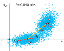
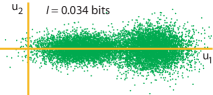
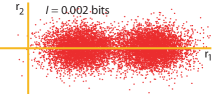
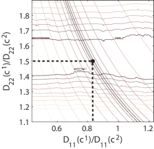
Figure 2: Unfolding and local equalization are optimal in multi-information and in achieving uniform population per unit-volume cluster. Top left plot shows a simple curved manifold, which was generated from particular misalignments $\alpha_{1}=10^{o}$, $\alpha_{2}=20^{o}$, and $\theta_{1}=30^{o}$, and particular ratios among the standard deviations in the local principal directions, namely $0.83$ and $1.5$. The effect of varying the parameters of the unfolding transform $U$ in reducing mutual information, $\Delta I$, is shown in the right top plot (darker means higher $\Delta I$). Middle left plot shows the same data under the identified optimal $U(\mathbf{x})$, and bottom left plot shows the data that jointly minimize $I$ while achieve uniform density clusters. The bottom right plot displays $I$ and iso-density contours (see text for details). The latent values are correctly identified by minimizing $I$ while enforcing uniform PDF. Conversely, unfolding along a PC, local model alignment and local equalization minimize $I$.

However, the variance of each local cluster may still depend on the location along the unfolded PC. This residual dependence can be removed by locally expanding or contracting the unfolded domain through an appropriate point dependent metric: $\mathbf{r}=D(\mathbf{x})\cdot U(\mathbf{x})$. Horizontal contour lines at the bottom right plot show the $I$ values for different combinations of metric changes applied at each cluster. Multi-information by itself does not completely constrain the line element along the unfolded dimension. However, if one additionally requires constant probability in the transformed domain (clusters of uniform volume), the solution is unique as shown by the combination of multi-information contours and the curved contours indicating uniform volume clusters. The minimum $I$ condition together with the equal volume condition (black dot) is obtained when the first cluster is vertically expanded to have the same height as the second cluster. As intuitively expected, the optimal local expansion or contraction in $I$ terms and in achieving constant volume regions is the one that makes the clusters equal (bottom left figure).

In a more general $d$-dimensional scenario, the required additional processing after unfolding along a Principal Curve could be setting the line element for local equalization in every direction of the orthogonal subspaces. This would achieve a constant (uniform) PDF along the curve thus ensuring the equality of all higher order moments. In 2-$d$ settings (as the one above) orthogonal subspaces are 1-$d$ and the additional equalization required after unfolding can be easily solved. Unfortunately, in general, orthogonal subspaces have dimension $(d-1)$, and the solution of multivariate equalization is not unique [62, 63]. A suboptimal alternative is performing the required equalization sequentially: following one secondary PC at a time. Therefore, unfolding and point-dependent equalization can be extended dimension-wise by sequentially drawing additional locally orthogonal PCs.

Even though a sequential (dimension-wise) procedure does not guarantee complete independence, equalization along secondary PCs is more sensible than using arbitrary linear directions since, according to their definition [48], they capture the main structure in the orthogonal subspaces. Moreover, the benefits of unfolding and point-dependent metric suggested so far, trivially generalize to more complicated manifolds that can be locally decomposed into clusters, as commonly assumed in the literature [40, 41, 42, 43, 3].

Accordingly, unfolding along PCs and the use of local metrics will be the basic processing elements of the proposed technique.

IV Sequential Principal Curves Analysis

The proposed transform consists of (1) certain differential behavior, and (2) certain integration path for this Jacobian.

IV-A Proposed differential behavior (Jacobian).

Local unfolding and equalization along PCs, can be expressed as:

$$\nabla R({\bf x})=D({\bf x})\cdot\nabla U({\bf x})$$ (10)

where ${\bf u}=U({\bf x})$ is the unfolding transform that consists of concatenated local rotations along the proposed path made of a sequence of PCs, and the diagonal matrix $D({\bf x})$ represents the local length of the line element along this path (change of metric). Note that $\nabla U({\bf x})$ is orthonormal for all ${\bf x}$ since the unfolding $U$ can be formulated as a set of concatenated local rotations. In fact, in agreement with [48, 50, 51], the method we (instrumentally) use here to draw local-to-global PCs relies on local PCA to estimate the tangent to the curve (see Appendix). Note that using local-PCA to compute PCs is consistent with the assumption of local Gaussian clusters, which is usual in the literature [40, 41, 42, 43, 3].

In order to adapt the metric to the density, we set the elements of $D$ using the marginal PDF on the unfolded coordinates and an appropriate exponent $\gamma\geq 0$:

$$D({\bf u})_{ii}\propto p_{u_{i}}(u_{i})^{\gamma}$$ (11)

where each marginal PDF is estimated following $k$-neighbors rule. The induced metric is: $M({\bf x})=\nabla U({\bf x})^{\top}\cdot D({\bf x})^{2}\cdot\nabla U({\bf x})$. Assuming that local clusters can be factorized by the local rotations (e.g. $\nabla U({\bf x})$ are local PCAs), we have:

$$\begin{array}[]{ll}|M({\bf x})|&=|D({\bf x})|^{2}\propto\prod_{i=1}^{n}p_{u_{i}}(u_{i})^{2\gamma}=p({\bf u})^{2\gamma}\\[8.53581pt] &=p({\bf x})^{2\gamma}|\nabla U({\bf x})|^{-2\gamma}=p({\bf x})^{2\gamma},\end{array}$$ (14)

which is the behavior required in Eq. (4) and encompasses both infomax and error minimization depending on $\gamma$.

IV-B Proposed integration path.

Given an arbitrary origin on the first PC, ${\bf x}^{o}$, assumed to give zero response, ${\bf r}^{o}={\bf 0}$, and some point of interest, ${\bf x}$; the transform $R(\bf{x})$ will be given by the integration of the proposed Jacobian along certain integration path from ${\bf x}^{o}$ to ${\bf x}$. As illustrated in Fig. 1, the proposed path is made of segments of the first and secondary PCs. The first PC is just the standard PC of the set [49], while secondary PCs were introduced in [48]. In the proposed path, the $i$-th PC is followed up to the geodesic projection of the point ${\bf x}$ on this PC, ${{\bf x}_{\bot}^{i}}$. Here geodesic projections are understood as projections that follow the local structure of the manifold. Geodesic projections are obtained from orthogonal projections according to the procedure described later.

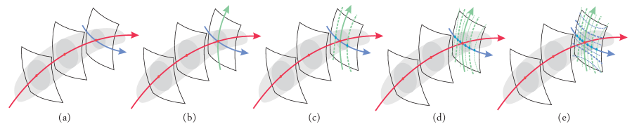
Figure 3: Curved locally orthogonal subspaces from secondary PCs and the appropriate PDF-dependent metric. Delicado’s secondary PCs (e.g. second PC in blue and third PC in green in a and b) capture the structure in the orthogonal subspace with regard to the Hastie’s PC (in red). A locally orthogonal curved subspace can be defined by considering additional 3rd PC curves at certain points on the 2nd PC (dashed and dotted green curves in c and e). Taking these points to be separated by constant cumulated density, as would be given by constant steps in $r_{2}$ (or integrated metric in 2nd dimension), the 3rd PCs divide the subspace in regions of constant population. If the same procedure is applied on the remaining dimensions (blue PCs in e), one obtains the lattice with constant population in each non-uniform cell, as in Fig. 1.

IV-C Direct Transform.

The SPCA transform of $\bf{x}$ is given by integrating the proposed $\nabla R$ along the proposed path:

$${\bf r}=R({\bf x})=C\cdot\int_{{\bf x}^{o}}^{{\bf x}}\nabla R({\bf x^{\prime}})\cdot d{\bf x^{\prime}}=C\cdot\int_{{\bf x}^{o}}^{{\bf x}}D({\bf x^{\prime}})\cdot\nabla U({\bf x^{\prime}})\cdot d{\bf x^{\prime}}\\$$ (15)

where $C$ is just a constant diagonal matrix that independently scales each component of the response. The selected path implies displacements in one PC at a time. According to this, the vector $d{\bf u^{\prime}}=\nabla U({\bf x^{\prime}})d{\bf x^{\prime}}$ has only one non-zero component: the one corresponding to the considered PC at the considered segment. Therefore, the response of each sensor to the point ${\bf x}$ is just the length on each PC in the path, measured according to the metric related to the local PDF with the selected $\gamma$,

$$r_{i}=C_{ii}\cdot\int_{{\bf x}_{\bot}^{i-1}}^{{\bf x}_{\bot}^{i}}D({\bf x^{\prime}})\cdot\nabla U({\bf x^{\prime}})\cdot d{\bf x^{\prime}}=C_{ii}\int_{0}^{u_{i\bot}^{i}}p_{u_{i}}(u^{\prime}_{i})^{\gamma}\,du^{\prime}_{i}\\$$ (16)

The scaling constants, $C_{ii}$, are a global response ranking.

SPCA is initialized by setting (i) the origin of the coordinate system, and (ii) the scale of the different dimensions and the order in which they will be visited by the sequential algorithm. Sensible choices for the origin are those suggested in other local-to-global PC algorithms [48, 50, 51]: the most dense point of the distribution (if known) or the mean of the data. Then a set of $d$ locally orthogonal PCs is drawn at the selected origin, which will be used to set the order and the relative scale of the dimensions. In our case, we set the scaling constants $C_{ii}$ according to an information distribution criterion: we use the number of quantization bins per dimension given by classical bit allocation results in transform coding [7], i.e higher marginal entropy first. Other criteria could be used, as for instance the total standard deviation of the projected data (as in global PCA) or the total Euclidean length of the curvilinear axes.

IV-D Inverse Transform.

Given a set of training samples from the source, the origin in the input space, ${\bf x}^{o}$, and the initialization (dimension order and scale), the computation of the inverse, ${\bf x}=R^{-1}({\bf r})$, is simple. It just involves drawing the first PC through the origin and taking the length $r_{1}$ on this curve, measured according to $p_{u_{1}}(u_{1})^{\gamma}$. Displacement on the first curve by the length $r_{1}$ leads to the first projection ${{\bf x}_{\bot}^{1}}$. Then, the second locally orthogonal curve is drawn from ${{\bf x}_{\bot}^{1}}$, and one takes a second displacement $r_{2}$ on this second PC leading to the second projection, ${{\bf x}_{\bot}^{2}}$. This process is repeated sequentially in every dimension until the point ${\bf x}$ is found by taking the displacement $r_{d}$ from ${\bf x}^{d-1}_{\bot}$ on the d-th PC.

Out-of-sample. Note that the transform can be easily applied to new samples (eqs. 15 and 16) as long as they are not too far from the training samples, i.e. as long as they come from the same source.

The reminder of the section is devoted to show how the concept of secondary PCs in [48] together with the local metric proposed here can be used to define (1) locally orthogonal subspaces, and (2) projections following the local structure of the manifold, which we called geodesic projections above. These are the ingredients behind the proposed SPCA path.

IV-E Locally orthogonal subspaces.

Hastie’s first PC summarizes the whole dataset [49]. Then, one may consider hyperplanes orthogonal to this first PC and local basis at those hyperplanes to describe the residuals. In principle, any set of ($d-1$) linearly independent vectors living in the corresponding hyperplane would suffice. However, as noted by Delicado [48], the residual at those hyperplanes may also have a curved structure. Therefore, it makes sense to draw a secondary PC at the hyperplane to capture this structure (e.g. blue curve in Fig. 3.a). Fig. 3 shows how the secondary PCs idea together with the proposed PDF-dependent metric can be used to define the lattice assumed in Fig. 1.

Even though SPCA does not require its explicit computation, such underlying lattice following the structure of the PDF illustrates the equalization properties of the SPCA representation. Delicado lists a set of conditions for these secondary PCs to exist [48]. A rigorous application of SPCA should start by checking that Delicado’s conditions hold for the dataset at hand. In Section V we take an empirical approach and show that in practice SPCA does induce the kind of PDF-dependent curvilinear lattices assumed in this section.

IV-F Geodesic projections.

In order to reach the target $\bf{x}$ following the structure of the manifolds (e.g. through geodesics) Delicado’s secondary PCs are drawn from certain projections on the 1st, 2nd, … PCs. If orthogonal projections are used, in general the target is not reached by the PCs. Fig. 4 describes the proposed iterative procedure to reach the target. The idea is modifying the current projections (or lengths $r_{i}$) to reduce the approximation error. At iteration $k$ we have:

$$\begin{array}[]{ll}{\bf r}(k+1)={\bf r}(k)+\alpha\,\boldsymbol{\delta}(k)\\[2.84526pt] \boldsymbol{\delta}(k)=C\cdot D({\bf x}_{\bot}^{d}(k))\cdot\nabla U({\bf x}_{\bot}^{d}(k))\cdot({\bf x}_{\bot}^{d}(k)-{\bf x})\end{array}$$ (19)

Results in synthetic and real manifolds in section V confirm the practical convergence of the geodesic projection thus leading to accurate transforms and inverses.

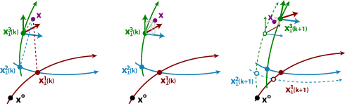
Figure 4: Iterative procedure to find the geodesic projections of the point to be transformed ${\bf x}$. In the first iteration the orthogonal projection is used as starting point for each secondary PC of the sequence (left plot). However, in general, the target point is not reached by drawing secondary PCs from the orthogonal projections. The residual from attempt $k$ to reach the point, ${\bf x}_{\bot}^{d}(k)-{\bf x}$, can be expressed in the local linear coordinates at the approximated point (center plot). The components of the residual in the local representation can be used to correct the position of the estimated projection on the curves, Eq. 19. At the new corrected projections, new local secondary PCs are drawn. The resulting path gets closer to the target (right plot).

V Experiments and Examples

In this section we focus on the intrinsic properties of SPCA which are independent of the algorithm to draw individual PCs. According to this, in each experiment we assume that that the algorithm chosen to draw individual PCs is tuned to the manifold at hand. In our case, this reduces to the minimization of the projection error (see Appendix). An implementation of SPCA with worked examples reproducing all the results of the work is available at http://isp.uv.es/spca.html.

The foundations of SPCA and its applications are analyzed in four sets of experiments:

• Underlying assumptions in SPCA. These experiments are intended to illustrate that the statements in Section IV actually hold in practice: (1) the concept of secondary PCs of Delicado can be used to define locally orthogonal subspaces and geodesic projections, and (2) the iterative procedure to get the geodesic projections converges giving rise to a transform with accurate inverse. We check this in synthetic data and in two kinds of real data: color manifolds and image (spatial texture) manifolds.

• Unfolding, Nonlinear ICA and Transform Coding. These experiments show that tuning the SPCA metric leads either to (1) plain unfolding, (2) identification of nonlinear independent components, or (3) optimal transform coding. We check this both in synthetic data and in image texture data.

• Dimensionality reduction. The performance of SPCA is compared to standard manifold learning techniques in a noisy swiss roll.

• Domain Adaptation. The performance of SPCA to find a meaningful canonical representation for manifold alignment is compared to PCA + whitening in a color constancy application.

• Classification: generalization of Mahalanobis distance. The manifold dependent metric associated to SPCA can be used in classification problems (e.g. k-nearest neighbors) as alternative to Mahalanobis distance.

V-A Underlying assumptions in SPCA

Locally orthogonal subspaces and geodesic projections. Figures 5 and 6 shows 2D and 3D examples of how the described SPCA procedure identifies curved subspaces which are locally orthogonal to the first PC.

In Fig. 5 we synthesized samples using marginal PDFs of increasing variance along a spiral. In a part of the spiral we used a Laplacian marginal, giving rise to a clear ridge in the manifold, while in the other part we used a uniform marginal. 1000 samples of such manifold were used for training. Here we show orthogonal subspaces computed at linearly spaced steps using SPCA with Euclidean metric ($\gamma=0$) and different origin points $\mathbf{x_{0}}$ on the first PC (highlighted dot on the red curve). Results show that (1) Euclidean metric does imply uniform spacing along the first PC (independent of the local PDF), (2) results are fairly independent of the chosen origin $\mathbf{x_{0}}$, and (3) identified subspaces display meaningful curvature so that samples far from the first PC are projected onto the first PC following the local PDF. Examples of Fig. 8, below, confirm that SPCA appropriately identifies subspaces and their distribution along the manifold for other metric choices.

Fig. 6 shows examples of the identified subspaces with the non-stationary manifolds used by Delicado to define the concept of secondary Principal Curves [48].

These results illustrate the fact that Delicado’s conditions for the existence of secondary PCs hold in practice for smooth manifolds (even displaying strong curvature) and the fact that these secondary PCs can be used to define locally orthogonal subspaces and geodesic projections as proposed in Section IV.

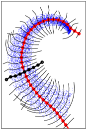
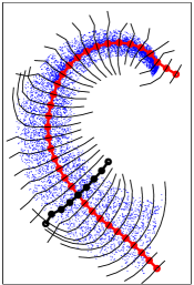
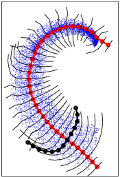
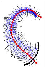
Figure 5: Locally orthogonal subspaces (in black) and geodesic projections (e.g. along black curves) are independent of the selected origin of coordinates (highlighted dots on the red curve).

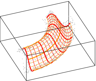
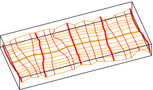
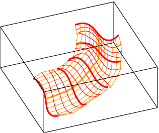
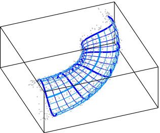
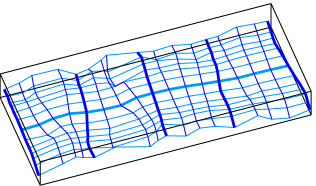
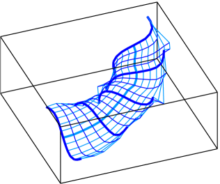
Figure 6: Locally orthogonal subspaces (curves in dark color) along the first Principal Curve (bold curve in light color) in Delicado’s manifolds [48]: the one in red with fixed locally orthogonal subspaces and the one in blue with twisted orthogonal subspaces. Left: Theoretical model and noisy data. Center: Original features in the SPCA transform domain (unfolding). Right: SPCA features (cartesian reticle in the transform domain) back in the input domain.

Color Data	Spatial Texture Data		Convergence

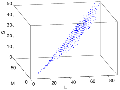
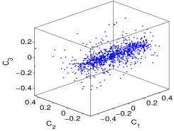
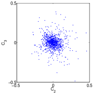
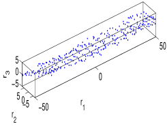
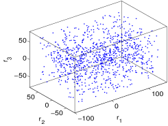
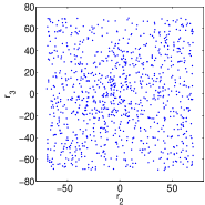
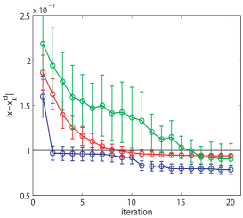
Figure 7: Convergence of the transform (accuracy of the proposed path through the geodesic projections). Top, transformed test points from the synthetic 2d manifold (left) and the real 3d color set (right). Euclidean metric $\gamma=0$ was used in the synthetic case and infomax metric $\gamma=1$ was used in the color case. Points highlighted in red are those that require iterative search since the residual is bigger than some accuracy threshold (in these examples 0.001 times the maximum Euclidean distance). Bottom, residuals as a function of the iterations in the computation of the path. Convergence saturates since iterations stopped once the accuracy threshold was reached.

Convergence. The ability to reach any point in the manifold using the proposed path through the geodesic projections (Eq. 19 and Fig. 4) is the key to obtain meaningful transforms with accurate inverse. Here we check the convergence of such procedure in three cases: (1) the synthetic manifold considered above, (2) tristimulus color data from a calibrated color image database [1], and (3) spatial texture -luminance only- data from another calibrated color image database [65].

Figure 7 -top row in left and central panels- shows the shape of the manifolds coming from real data. The color manifold in LMS space (long, medium and short wavelength) displays the classical correlation between tristimulus components [15, 66, 1]. Figure shows 300 test color samples, but 20000 samples were used for training. The spatial texture data come from $15\times 15$ luminance patches. PCA rotation and whitening was applied to these patches (225-dimensional vectors). PCA was computed using $2.5\cdot 10^{6}$ samples. Then, 15000 particular image samples were selected for training falling close to a particular 3d subspace (only 3 active PCA components and the rest close to zero). 1000 test samples are shown at the top of the central panel. Axes are named as $C_{i}$ for contrast of each PCA component. The image texture samples show the classical elongation along the first principal component and the sparse elliptical symmetry in the other dimensions [67, 68].

In all cases (synthetic data, color data and texture data), test points were transformed using SPCA using different metrics ($\gamma=0$ for the synthetic and color data, and $\gamma=1$, i.e. equalization, for the texture data). Original and transformed (unfolded) synthetic data are omitted in Fig. 7 since they are shown in Fig. 8. Real data transformed are shown in the bottom row of the left and central panels in Fig. 7. Note that $\gamma=1$ achieves component independence as predicted by the theory.

In these examples, the iteration described in Eq. 19 stopped when the reconstruction error $|\mathbf{x}-\mathbf{x}_{\bot}^{d}|$ was smaller than a fraction of the maximum Euclidean distance in the manifold.

In the experiments, a large fraction of test points is reached within the accuracy threshold in a single iteration. Figure 7 shows the evolution of the reconstruction error for the points that were not reached in the first iteration. In our implementation, the convergence constant $\alpha$ in Eq. 19 was set to 0.01. However, faster convergence results and improved accuracy could be obtained with adaptive $\alpha$ as in gradient descent procedures [69]. The aim of these convergence examples is just to illustrate that the transform works in practical situations: in the proposed examples, accurate direct and inverse transforms are obtained within less than 15 iterations of the algorithm. Note that convergence saturates since the iteration for each point stopped once the accuracy threshold was reached.

V-B Unfolding, Nonlinear ICA and Transform Coding

Synthetic example. The advantage of using PCs to design a set of sensors is that their flexibility makes them suitable to describe curved manifolds, as pointed out in Fig. 8. No matter the metric used, an unwrapped representation of the data is obtained. When using $\gamma=0$ the data is unfolded and the original local metric is preserved (e.g. the different distributions inside the manifold remain the same). When using $\gamma=1$, we obtain a representation where the different distributions are almost uniformized, leading to a representation where the different dimensions are almost independent. Finally, when using $\gamma=\frac{1}{3}$, the reconstruction error is minimized. In this latter case, redundancy is certainly reduced with regard to the input domain, however, the kurtotic structure of the Laplacian is more visible than in the second case. Note also the differences in the distribution of the inverted lattices: while in the $\gamma=0$ case, lattice cells are approximately uniform no matter the local population (local metric independent of the PDF), in the other cases, the size is related to the population, e.g. the $\gamma=1$ case results in tighter slices around the peak of the Laplacian distribution. As anticipated in Section III, unfolding alone ($\gamma=0$) is not enough to remove redundancies in general, but incorporating local changes in the metric can achieve independent components.

$\gamma=0$	$\gamma=1/3$	$\gamma=1$
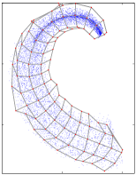
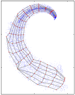
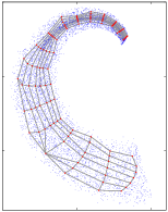
$MI$ (bits) 0.27	0.06	0.05
RMSE 0.55	0.53	0.56

Figure 8: Infomax or error minimization through SPCA. The sets in the first row were transformed using SPCA (second row) with different $\gamma$ values. Additionally, Cartesian lattices in the response domain were inverted back into the input domain leading to the curved lattices in the top row. Results are analyzed in terms of independence (Mutual Information), and reconstruction error (RMSE). In each case, MI was computed in the transform domain, while RMSE values refer to the quantization error in the input domain using the corresponding lattices as codebook. For reference, in the original domain results were $MI=0.75$ bits and RMSE=$0.63$ (using uniform scalar quantization). Note how $\gamma=1$ obtains better results in independence while $\gamma=\frac{1}{3}$ is better for RMSE minimization. The Euclidean choice, $\gamma=0$, leads to constant-size cells independent of the PDF.

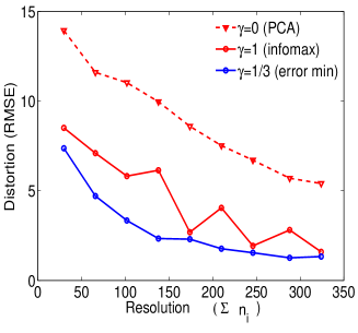
Original	PCA
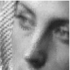
SPCA ($\gamma=1$)	SPCA ($\gamma=1/3$)

Figure 9: Image coding results. Top: Resolution-Distortion plot. Bottom: reconstructed images using the same resolution ($\sum_{i}n_{i}=66$) in different representations.

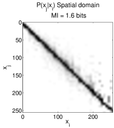
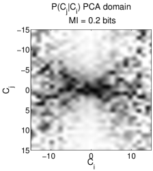
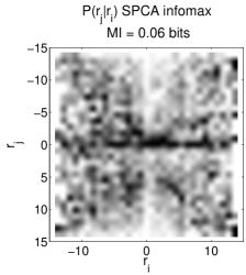
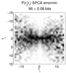
Figure 10: Conditional PDFs and quantitative independence measures in the considered domains. Top: spatial domain (left) and PCA domain (right). Bottom: SPCA $\gamma=1$ (left) and SPCA $\gamma=1/3$ (right). Note that bigger Mutual Information values are consistent with visible (correlation or bow-tie) structures in the conditional probabilities.

Encoding spatial texture. Efficient representation of spatial information is a challenging problem for manifold learning techniques and a suitable scenario to check the effect of different optimality criteria. In this section the training set consists of $2\cdot 10^{5}$ 4-dimensional vectors from $2\times 2$ luminance patches of natural images from the calibrated McGill database [65]. SPCA was trained on these samples in the PCA domain using $\gamma=1$ and $\gamma=1/3$ metrics. Note that given the symmetry of image data, plain unfolding, i.e. $\gamma=0$, is very similar to PCA. SPCA was then applied to 1500 test samples from the McGill database and to 2500 samples from the standard image Barbara (not included in the training set).

The ability of SPCA for transform coding is illustrated by using sensors with limited resolution (uniform quantization in each dimension of the transformed domain) in the considered representations. In every case, resolution in each dimension was set according to standard bit allocation [7]. Figure 9 shows the reconstruction error as a function of the resolution of the sensors for 60 randomly chosen samples from the Barbara image. Figure 9 also shows reconstructed images from the quantized representations using the same sensor resolution (number of quantization bins). The resolution-distortion plot shows that SPCA with the error minimization metric substantially reduces the RMSE in image coding with regard to Euclidean metric ($\gamma=0$, or uniform quantization of PCA) and to the infomax SPCA. The decoded images show the practical relevance of the numerical gain achieved by the non-Euclidean $\gamma=1/3$ approach.

The ability of SPCA for nonlinear ICA is qualitatively and quantitatively assessed by inspecting the conditional PDFs between AC coefficients (as in [20, 21, 26]) and by the corresponding mutual information (MI) measures (see Fig. 10). Bow-tie structures in the conditional PDFs and MI measures in the spatial domain and in the PCA domain are consistent with previously reported results for natural images [26]. Uniform conditional PDF and small MI show that SPCA with the infomax metric strongly reduces the redundancy between the coefficients of the representation. On the contrary, in the case of SPCA with the error minimization metric the bow-tie shape is still visible in the conditional PDF.

These results confirm the theoretical prediction that SPCA can be tuned either for infomax (using $\gamma=1$) or for error minimization (using $\gamma=1/3$).

V-C Dimensionality reduction

SPCA $\gamma$ = 0	SPCA $\gamma$ = 1/3	SPCA $\gamma=1$	LLE	Isomap	Charting

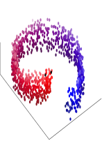
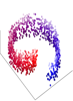
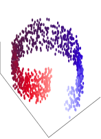
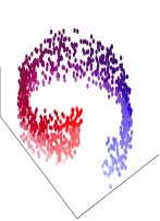
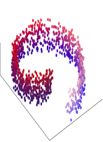
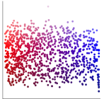
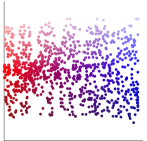
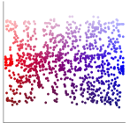
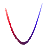
Figure 11: Dimensionality reduction (from 3d to 2d): unfolding a noisy swiss roll with SPCA using different metrics, LLE, Isomap and Charting. In every case, $2000$ samples were used to learn the reduced dimensionality responses. The number of nearest neighbors in LLE and Isomap was varied in the range [$2,50$], and the number of local models in charting was varied in the range [$2,50$]. We show the solutions with best qualitative performance. As stated above, in the SPCA cases, the parameters of the algorithm to draw individual PCs were chosen to minimize the reconstruction error (see Appendix).

Dimensionality reduction with SPCA consists of considering $d^{\prime}<d$ components of the response vector. Figure 11 shows the qualitative performance of SPCA in dimensionality reduction by unfolding a noisy version of the popular 2d swiss roll embedded in $\mathbb{R}^{3}$. We compare SPCA to the solutions given by other popular dimensionality reduction methods such as those based on geodesic computation (Isomap [47]), spectral methods (LLE [34]), and local model coordination (charting [43]).

Bottom row of Fig. 11 shows the scatter plot of the samples according to the coordinates identified by each algorithm. In this transformed domain the variation in the first dimension is depicted with a hue change from red to blue, while the variation in the second dimension is depicted with a luminance change from dark to bright. Top row of Fig. 11 shows the samples in the original domain colored according to the color code found in the transformed domain. Therefore, the quality of the curvilinear coordinates can be evaluated in two ways: (1) by assessing the shape of the unfolded sets of samples, and (2) by assessing the meaningfulness of the color distribution in the original domain.

SPCA $\gamma$ = 0	SPCA $\gamma$ = 1/3	SPCA $\gamma=1$

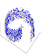
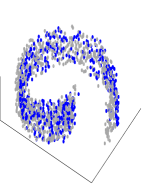
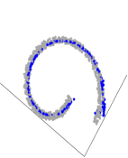
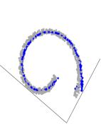
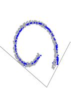
Figure 12: Original samples (in gray) and SPCA samples with reduced dimensionality projected back into the original domain (in blue). Top and bottom row show the same data from different view points to illustrate the fact that, no matter the metric strategy, the inverse of SPCA properly identifies the underlying 2d manifold.

It is observed a heavy warping of the tails of the embedding for LLE. As a result, the second (dark/bright) dimension has no meaning in the input domain. Color distribution (meaning of dimensions) is consistent in Isomap and the SPCA results no matter the selected metric: the first (hue) dimension means angular position and the second (luminance) dimension means height for a fixed angular position. It is reasonable that SPCA (which sorts the dimensions according to entropy or variance) gives rise to the same dimension sorting as Isomap, which considers the length of the geodesics. In this example the length (and the variance) along the angular dimension is bigger than in the other dimension. On the contrary, the sorting in the case of charting is the opposite. Finally, it is worth to stress that SPCA (no matter the metric) gives rise to more regular and uniform scatter plots in the transform domain.

On top of improved data visualization, the invertibility of SPCA allows to project the low dimensional samples back into the original domain revealing the latent manifold, Fig. 12.

V-D Domain Adaptation

Color constancy under change of observation conditions is a challenge for machine learning techniques because it involves strong changes in the samples coming from the same physical objects. Changes in linear measurements (tristimulus values) may arise from changes in the spectral illumination and from changes in the geometry of surfaces and light sources. In general such changes are non-linear, specially those coming from geometry changes, so they cannot be compensated through linear techniques. The examples of the top row of Fig. 13 show two pictures of similar objects illuminated with different spectral radiance (CIE D65, left and CIE A, right) under different illumination angles. The differences in spectral radiance induce a rotation of the manifold in the color space, and the change of surface and illumination geometry induce the presence of shadows. This latter effect results in a different distribution of samples within the PDF support. In the CIE A case the low luminance region is relatively more populated. According to this, color constancy is an appropriate problem to assess the ability of a manifold learning technique in (non-linear) domain adaptation. In this section, we apply the proposed method for color compensation, or more specifically for manifold matching, as an example of domain adaptation. We compare the results with a classical linear technique for chromatic adaptation based on PCA and whitening [70].

Our strategy for domain adaptation is related to the corresponding pair procedure, which has been proposed in the computational color vision literature using psychophysically-based models [71]. Given a color vision model, ${\mathcal{M}}$, that describes the perception, $P$, of a test, $K$, in some adaptation state (e.g. under observation conditions, $S$), $P={\mathcal{M}}(K,S)$, the corresponding pair, $K^{\prime}$ in a different adaptation state, $S^{\prime}$, is given by [71]:

$$K^{\prime}={\mathcal{M}}^{-1}({\mathcal{M}}(K,S),S^{\prime}).$$ (20)

In our manifold learning context, this reduces to considering the color statistics of natural scenes under illuminations $S$ and $S^{\prime}$. Then, the $K$ test points are transformed using SPCA with the set of colors under illumination $S$, and inverted back using the set of colors under $S^{\prime}$. The match between invariant (adapted) representations obtained using SPCA from different linear (variant) representations, as suggested by Eq. (20), is related to the nonlinear canonical correlation analysis [41].

As shown in Fig. 13, linear transforms can compensate the rotation due to the spectral radiance change but the resulting set is still biased towards the low luminance region. The diagram in Fig. 13 illustrates the procedure for color compensation using SPCA. Transforms leading to the corresponding latent coordinates of the manifold in the environments $A$ and $B$ may be used to estimate the position in environment $A$ of new points measured in environment $B$. Unlike in the linear adaptation case above, the proposed nonlinear transform not only removes the yellowish appearance, but additionally reduces the shadows, as expected from a better PDF matching. In particular, note how the highlighted point $\mathbf{x}_{B}$ (the same one as above) results in a white, higher luminance corresponding point $\mathbf{\hat{x}}_{A}$.

Environment A:	Environment B:
CIE D65 illumination	CIE A illumination
Linear Measurements and PCA+whitening Manifold Matching
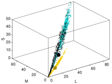
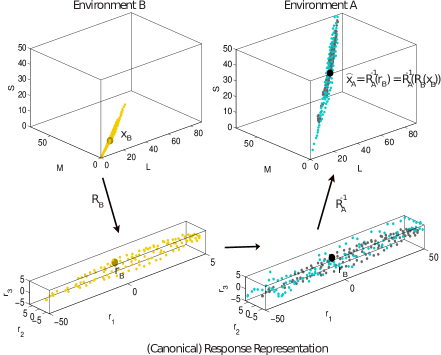
PCA+whitening	SPCA

Figure 13: Dataset shift compensation by using the corresponding pair concept and SPCA. First row: similar objects acquired in different spectral and geometry illumination conditions. Second row: manifolds of the colors in the two images are shown in blue (CIE D65) and in yellow (CIE A). In black we plot the colors of CIE A after color compensation using PCA+whitening. One particular color in the CIE A case has been highlighted (large yellow dot). The corresponding corrected color has been highlighted in black. Diagram in the third row: procedure for color compensation using SPCA. The key for color compensation is inverting the transform of points acquired in the B environment (gray points) using the inverse of the transform learned for the samples acquired in the A environment. Bottom row: reconstructed images after color compensation by PCA+whitening and the proposed SPCA.

V-E SPCA in classification

The manifold dependent metric associated to SPCA (Eq. 10 4) can be used in classification problems (e.g. k-nearest neighbors) as alternative to Mahalanobis distance. Euclidean distance in the whitened SPCA domain is a generalization of Mahalanobis metric (which is the Euclidean distance in the whitened PCA domain). Similar generalizations can be done with the related methods Principal Polynomial Analysis (PPA) [4] and Dimensionality Reduction via Regression (DRR) [5].

An example of how this kind of metrics can benefit the classification can be found in [4] (Figs. 3 and 4), where we used PPA. The reason is that given a sample, the loci of equidistant neighbors is an ellipsoid which is oriented according to the local structure of the manifold (and not a sphere). This minimizes the number of wrong-class samples in the selected neighbors. On top of this advantage (shared by PPA-based and DRR-based metrics), SPCA-based may be even better since discrimination will be higher in high density regions thus reducing the average misclassification error.

VI Summary

Here we introduced the full technical details of Sequential Principal Curves Analysis [1, 2]. It is a nonlinear feature extraction method appropriate to design artificial sensory systems and to analyze the rationale of biological sensory systems. See also [3, 4, 5] for prequels and sequels.

Here we introduced the general technical motivations of SPCA: data unfolding along PCs, followed by local metric change leads to to easily interpretable nonlinear independent components. Moreover, splitting the infomax problem into two stages (unfolding and equalization) allows us to propose data representations guided by alternative optimization criteria such as error minimization. SPCA can be seen as a particular solution to the design of optimal feature extraction for either independence or transform coding when imposing the preservation of local geometry in addition to the infomax or the error minimization goals. Following the first and secondary PCs of the manifold ensures the interpretability of the identified features, as opposed to spectral, kernel, projection-pursuit, and neural networks methods for manifold learning.

We explicitly checked the underlying assumptions of SPCA in synthetic and real examples: (1) secondary PCs can be used to define locally orthogonal subspaces, (2) the proposed transform converges so that SPCA is invertible, and (3) nonlinear ICA and optimal transform coding are available using SPCA by choosing the appropriate metric. We showed examples of the use of SPCA in dimensionality reduction, domain adaptation, and classification (by generalizing the Mahalanobis distance).

VII Acknowledgements

This work has been supported by the Spanish Ministry for Science and Innovation under grants BFU2014-58776 and TIN2013-50520. The authors thank Gustau Camps-Valls and Gema Denia for their support before a conference presentation of SPCA [72].

VIII Appendix:
A bottom-up approach to draw
one Principal Curve

In this appendix we present a local-to-global algorithm to draw first [49] or secondary [48] Principal Curves. This is just an instrument to build the individual PCs required in the sequence followed in SPCA. This element of the general SPCA framework could be implemented with already reported bottom-up algorithms such as those in [48, 50, 51]. However, given the unavailability of Matlab working code, we developed our own algorithm where the local structure is analyzed in terms of local PCA.

The proposed PC algorithm follows a local-to-global or bottom-up approach since it identifies the local structure around the selected Principal Curve origin, and progressively builds the curve from that origin. In this appendix we show the geometric meaning of the parameters of the technique (instrumental parameters) and provide a particular procedure to tune them for the dataset at hand: the appropriate set of parameters is the one that minimizes the projection error onto the Principal Curve. This procedure is consistent with the original definition of Principal Curves and with the definition of Principal Components in linear PCA.

Algorithm. This procedure draws one PC from a specific point, ${\bf x}^{o}$, in a particular direction, $B^{i}$. The algorithm uses PCA to find linear directions that go through the middle of the dataset. Hence, the proposed PC consists of segments obtained using local PCAs.

The procedure starts from ${\bf x}^{o}$, where a local PCA is computed. Then, the most similar eigenvector to the desired direction is taken. The eigenvector is modified so that it points to the mean of the data in the direction ahead. The new point of the PC, ${\bf x}^{1}$, is obtained by making a step from ${\bf x}^{o}$ in the direction of the modified eigenvector. The obtained segment goes from ${\bf x}^{o}$ to ${\bf x}^{1}$. The rest of the curve points are obtained applying the same procedure departing from the new points until one of these stopping criteria is met: (1) if the distance between the new point, ${\bf x}^{n+1}$, and some of the previously drawn PCs is less than a threshold $\tau$, the algorithm stops since the current PC is almost crossing a previous PC, and (2) if the distance between the new point, ${\bf x}^{n+1}$, and all the points in the manifold is bigger than a given distance, $d_{out}$, the algorithm stops since ${\bf x}^{n+1}$ is assumed to be out of the manifold.

Specifically, each point ${\bf x}^{n+1}\in$ PC is computed from the previous point, ${\bf x}^{n}$, and the reference matrix, ${\bf B}_{n}$, following the procedure in Algorithm 1.

The parameters of the algorithm to draw one PC at a given point basically control the rigidity of the curve. These parameters include the size of the local neighborhood (set using the $k$-neighbors rule), the stiffness $q$, and the step size $\tau$ (see the table Algorithm 1).

Intuitively, the bigger the locality, the stiffness and the step size, the bigger the rigidity, so the obtained Principal Curves approach the global linear principal components, thus reducing the flexibility of the technique to describe curved manifolds.

Algorithm 1 Draw one Principal Curve at a given point.

  Input: dataset $\{{\bf x}^{i}|i=1,\ldots,N\}$

  Set parameters: Line increment $\tau$, stiffness $q$, and $k$ nearest neighbors

  Output: PC formed by a set of basis ${\bf B}_{n}$ and connected points

  1: Set origin at $n=0$, ${\bf x}^{o}$, and center the data in ${\bf x}^{o}$

  repeat

     2: Define a neighborhood around ${\bf x}^{n}$ according to the $k$-neighbors rule

     3: Compute PCA with the neighbors, obtaining eigenvectors ${\bf V}$

     4: Align and reorder ${\bf V}$ with the corresponding vectors in ${\bf B}_{n}$

     5: Compute the local mean ahead $\boldsymbol{\mu}$

     6: Modify ${\bf V}_{i}$ to point the local mean ahead: ${\bf V}_{i}^{\prime}={\bf V}_{i}+\frac{1}{q}\cdot\boldsymbol{\mu}$

     7: Compute the new point: ${\bf x}^{n+1}={\bf x}^{n}+\tau{\bf V}_{i}^{\prime}$

     8: Compute the new reference basis: ${\bf B}_{n+1}={\bf V}$

  until New point is outside the manifold or the PC crosses a previous PC

Effect of $k$-neighborhood: $\tau=1$, $q=10$
$k=1\%$	$k=10\%$	$k=30\%$
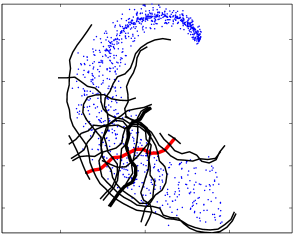
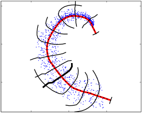
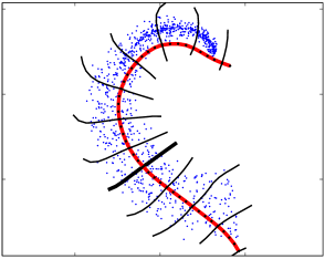
Effect of step size $\tau$: $k=10\%$, $q=10$
$\tau=0.02$	$\tau=1$	$\tau=3$
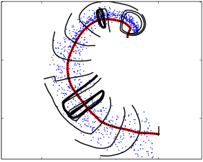
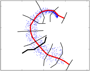
Effect of stiffness $q$: $k=10\%$, $\tau=1$
$q=2$	$q=10$	$q=\infty$

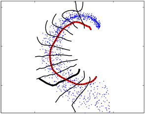
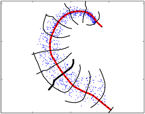
Figure 14: Effect of the $k$-rule (top), the step size $\tau$ (middle), and the stiffness $q$ (bottom) on the first and secondary PCs at different points. The first PC is shown in red and the secondary are plotted in black. The secondary PC at the selected origin of coordinates is in bold style. Note that in this example the crossing criterion is applied only between the first PC and each of the secondary PCs. The second row shows the data projected onto the first PC, which helps in assessing the committed unfolding errors.

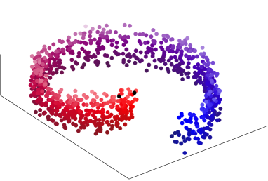
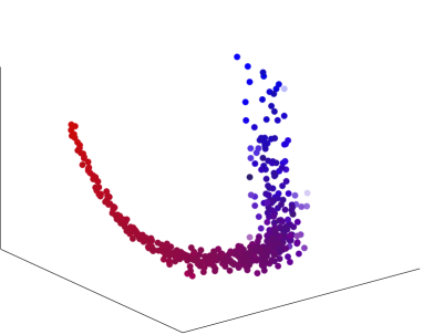
Figure 15: Manifolds for the parameter estimation experiment: noisy swiss roll (left), and noisy 1-d curve in a 3d-space (right)

.

Effect of instrumental Principal Curve parameters In this experiment we analyze the effect of the rigidity parameters. The experiment is done on a synthetic example of a challenging 2D manifold: noisy spiral data. We generated $10000$ samples from a curved manifold with changing PDF along the underlying PC: half of the manifold follows an increasing variance Laplacian distribution while the other half follows an increasing variance uniform distribution (Fig. 14).

As anticipated above, the rigidity of the PCs depends on different parameters: (2) the size of the $k$-rule neighborhood, (2) the step size, $\tau$, and (3) the stiffness parameter $q$. Some prescriptions to tune them are given below:

• The parameter $k$ determines the number of samples of the considered neighborhood for local PCA computation. Too small $k$ values give rise to noisy PCA estimates and hence the obtained PC becomes unstable, while too large $k$ values may give rise to neighborhoods which are not local enough and thus too rigid PCs are obtained. See Fig. 14[top] for the illustration of these effects.

• The step size, $\tau$, is the distance between the points where local basis are computed when drawing the PCs before setting the metric. Too large $\tau$ values give rise to too rigid PCs while too small values not only increase the computational time but also gives rise to unstable results: when the curve approaches one extreme of the manifold too small step size may cause unexpected turns, see Fig. 14[middle]. This parameter is given in Euclidean units in the input domain: if prior information on the maximum possible curvature for the manifold is available, this can be used to set the $\eta$ value conveniently.

• Finally (Fig. 14[bottom]), the stiffness controls the impact of the local mean ahead in the modification of the local PCA direction. Too small stiffness results on a big impact of the local mean, increased flexibility and unstable results. Too large stiffness implies neglecting the local mean which for big $\tau$ leads to too rigid solutions.

Fitting the instrumental Principal Curve parameters Different datasets may present different curvatures and inhomogeneities so different parameters of the algorithm may be needed. Here we present a criterion in order to tune the parameters of the algorithm for a particular dataset. This criterion is based on the definition of PC given in [49]: it is a self-consistent smooth curve which passes through the middle of a d-dimensional data cloud. In particular the parameters can be selected in order to minimize the distance between the data points and its projections on the drawn PC. This criterion is equivalent to minimize the reconstruction error obtained when using the PC for dimensionality reduction (reduction from dimension $d$ to dimension $1$), and it is also equivalent to minimize the variance in the subspace orthogonal to the PC which is the optimization criterion in classical (linear) Principal Component Analysis [54].

In order to show that different manifolds may require different parameters of the algorithm, in the following experiment we consider data from the manifolds shown in Fig. 15: swiss roll, and 1-d curve embedded in a 3-d space. Figures 16 and 17 show how the error varies depending on the parameters for the considered manifolds. The optimal parameters can be obtained from the minima (lighter points) in these surfaces. As apparent in the figures, these manifolds require different parameters to minimize the projection error.

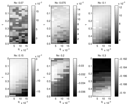
Figure 16: Projection error in the swiss roll example. Darker means more error. Each image is from different k-neighbors, inside each image the parameters $\tau$ and $q$ are modified.

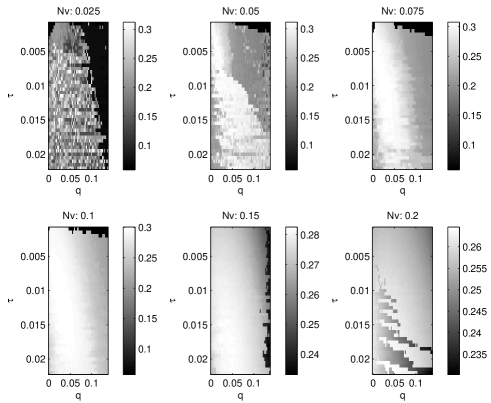
Figure 17: Projection error 1-d curve embedded in the 3-d space. Darker means more error. Each image is fro different k-neighbors, inside each image the parameters $\tau$ and $q$ are modified.

References

- [1] V. Laparra, S. Jiménez, G. Camps-Valls, and J. Malo, “Nonlinearities and adaptation of color vision from Sequential Principal Curves Analysis,” Neural Computation, vol. 24, no. 10, pp. 2751 –2788, 2012.
- [2] V. Laparra and J. Malo, “Visual aftereffects and sensory nonlinearities from a single statistical framework,” Front. Human Neurosci., vol. 9, 2015.
- [3] J. Malo and J. Gutiérrez, “V1 non-linear properties emerge from local-to-global non-linear ICA,” Network: Comp. Neur. Syst., vol. 17, no. 1, pp. 85–102, 2006.
- [4] V. Laparra, S. Jiménez, D. Tuia, G. Camps, and J. Malo, “Principal polynomial analysis,” Int. J. Neur. Syst., vol. 24, no. 6, pp. 1–21, 2014.
- [5] V. Laparra, J. Malo, and G. Camps, “Dimensionality reduction via regression in hyperspectral imagery,” IEEE J. Sel. Topics Sig. Proc., vol. 9, no. 9, 2015.
- [6] R.J. Clarke, Transform Coding of Images, Acad. Press, NY, 1985.
- [7] A. Gersho and R. M. Gray, Vector Quantization and Signal Compression, Kluwer, Boston, 1992.
- [8] P.J. Hancock, R.J. Baddeley, and L.S. Smith, “The principal components of natural images,” Network, vol. 3, no. 1, pp. 61–70, 1992.
- [9] D.S. Taubman and M.W. Marcellin, JPEG2000: Image Compression Fundamentals, Standards and Practice, Kluwer Academic Publishers, Boston, 2001.
- [10] D. G. Lowe, “Distinctive image features from scale-inveriant keypoints,” Intl. J. Comp. Vis., vol. 60, pp. 91–110, 2004.
- [11] J. Wright, Y. Ma, J. Mairal, G. Sapiro, T.S. Huang, and S. Yan, “Sparse representation for computer vision and pattern recognition,” Proc. IEEE, vol. 98, pp. 1031–1044, 2010.
- [12] B. A. Olshausen and D. J. Field, “Emergence of simple-cell receptive field properties by learning a sparse code for natural images,” Nature, vol. 381, pp. 607–609, 1996.
- [13] A. J. Bell and T. J. Sejnowski, “The ‘independent components’ of natural scenes are edge filters,” Vision Research, vol. 37, no. 23, pp. 3327–3338, 1997.
- [14] P.O. Hoyer and A. Hyvarinen, “Independent component analysis applied to feature extraction from colour and stereo images,” Network: Computation in Neural Systems, vol. 11, pp. 191–210, 2000.
- [15] E. P. Simoncelli and B. O. Olshausen, “Natural image statistics and neural representation.,” Annu. Rev. Neurosci., vol. 24, pp. 1193–1216, 2001.
- [16] E. Doi, T. Inui, T. Lee, T. Wachtler, and T. Sejnowski, “Spatiochromatic receptive field properties derived from information-theoretic analysis of cone mosaic responses to natural scenes,” Neural Computation, vol. 15, no. 2, pp. 397–417, 2003.
- [17] S. B. Laughlin, “Matching coding to scenes to enhance efficiency,” in In Braddick, O.J. & Sleigh, A.C. (Eds) Physical and Biological Processing of Images. 1983, pp. 42–52, Springer.
- [18] A. J. Bell and T. J. Sejnowski, “An information-maximization approach to blind separation and blind deconvolution,” Neural. Comput, vol. 7, no. 6, pp. 1129–1159, 1995.
- [19] E P Simoncelli, “Statistical models for images: Compression, restoration and synthesis,” in Proc 31st Asilomar Conf on Signals, Systems and Computers, Pacific Grove, CA, Nov 2-5 1997, vol. 1, pp. 673–678, IEEE Computer Society.
- [20] R. W. Buccigrossi and E.P. Simoncelli, “Image compression via joint statistical characterization in the wavelet domain,” IEEE Tr. Im. Proc., vol. 8, no. 12, pp. 1688–1701, 1999.
- [21] A. Hyvärinen, J. Hurri, and J. Väyrynen, “Bubbles: a unifying framework for low-level statistical properties of natural image sequences,” JOSA A, vol. 20, no. 7, pp. 1237–1252, 2003.
- [22] J. Malo, I. Epifanio, R. Navarro, and E. Simoncelli, “Non-linear image representation for efficient perceptual coding,” IEEE Tr. Im. Proc., vol. 15, no. 1, pp. 68–80, 2006.
- [23] J. Gutiérrez, F. Ferri, and J. Malo, “Regularization operators for natural images based on nonlinear perception models,” IEEE Tr. Im. Proc., vol. 15, pp. 189–200, 2006.
- [24] G. Camps, J. Gutiérrez, G. Gómez, and J. Malo, “On the suitable domain for SVM training in image coding.,” JMLR, vol. 9, pp. 49–66, 2008.
- [25] A. Hyvarinen, J. Hurri, and P. Hoyer, Natural Image Statistics: A Probabilistic Approach to Early Computational Vision., Springer, Berlin, 2009.
- [26] J. Malo and V. Laparra, “Psychophysically tuned divisive normalization approximately factorizes the PDF of natural images,” Neur. Comp., vol. 22, no. 12, pp. 3179–3206, 2010.
- [27] J. M. Foley, “Human luminance pattern mechanisms: Masking experiments require a new model,” JOSA, vol. 11, no. 6, pp. 1710–1719, 1994.
- [28] A. B. Watson and J. A. Solomon, “A model of visual contrast gain control and pattern masking,” JOSA A, vol. 14, pp. 2379–2391, 1997.
- [29] M. Carandini and D. J. Heeger, “Summation and division by neurons in visual cortex,” Science, vol. 264, pp. 1333–1336, 1994.
- [30] J. R. Cavanaugh, W. Bair, and J. A. Movshon, “Selectivity and spatial distribution of signals from the receptive field surround in macaque v1 neurons,” J. Neurophysiol, vol. 88, no. 5, pp. 2547–2556, 2002.
- [31] M. Carandini and D. Heeger, “Normalization as a canonical neural computation.,” Nature Reviews. Neurosci., vol. 13, no. 1, pp. 51–62, 2012.
- [32] I. Epifanio, J. Gutiérrez, and J.Malo, “Linear transform for simultaneous diagonalization of covariance and perceptual metric matrix in image coding,” Pattern Recognition, vol. 36, pp. 1799–1811, 2003.
- [33] V. Laparra, J. Muñoz Marí, and J. Malo, “Divisive normalization image quality metric revisited,” JOSA A, vol. 27, no. 4, pp. 852–864, 2010.
- [34] S. T. Roweis and L. K. Saul, “Nonlinear dimensionality reduction by locally linear embedding,” Science, vol. 290, no. 5500, pp. 2323–2326, December 2000.
- [35] M. Belkin and P. Niyogi, “Laplacian eigenmaps for dimensionality reduction and data representation,” Neural Computation, vol. 15, pp. 1373–1396, 2002.
- [36] K. Q. Weinberger and L. K. Saul, “Unsupervised learning of image manifolds by semidefinite programming,” in Proc. IEEE CVPR, 2004, pp. 988–995.
- [37] B Schölkopf, A J. Smola, and K-R. Müller, “Nonlinear component analysis as a kernel eigenvalue problem,” Neural Computation, vol. 10, no. 5, pp. 1299–1319, 1998.
- [38] C. J. C. Burges, “Geometry and Invariance in Kernel Based Methods,” in Advances in Kernel Methods: Support Vector Learning, B. Schölkopf, C. J. C. Burges, and A. J. Smola, Eds. MIT Press, 1999.
- [39] N. Kambhatla and T. Leen, “Dimension reduction by local PCA,” Neural Computation, vol. 9, pp. 1493–1500, 1997.
- [40] S. T. Roweis, L. K. Saul, and G. E. Hinton, “Global coordination of local linear models,” in Advances in Neural Information Processing Systems 14. 2002, pp. 889–896, MIT Press.
- [41] J. J. Verbeek, N. Vlassis, and B. Krose, “Coordinating principal component analyzers,” in In Proc. International Conference on Artificial Neural Networks. 2002, pp. 914–919, Springer.
- [42] Y. W. Teh and S. Roweis, “Automatic alignment of local representations,” in NIPS 15. 2003, pp. 841–848, MIT Press.
- [43] Matthew Brand, “Charting a manifold,” in NIPS 15. 2003, pp. 961–968, MIT Press.
- [44] J. Lin, “Factorizing probability density functions: Generalizing ICA,” in Proc. 1st Intl. Workshop on ICA and Signal Separation, 1999, pp. 313–318.
- [45] T. Kohonen, “Self-organized formation of topologically correct feature maps,” Biological Cybernetics, vol. 43, no. 1, pp. 59–69, January 1982.
- [46] C. M. Bishop, M. Svensén, and C. K. I. Williams, “GTM: The generative topographic mapping,” Neural Computation, vol. 10, pp. 215–234, 1998.
- [47] Joshua B. Tenenbaum, Vin Silva, and John C. Langford, “A global geometric framework for nonlinear dimensionality reduction,” Science, vol. 290, no. 5500, pp. 2319–2323, December 2000.
- [48] P. Delicado, “Another look at principal curves and surfaces,” J. Multivar. Anal., vol. 77, pp. 84–116, 2001.
- [49] T. Hastie and W. Stuetzle, “Principal curves,” J. Am. Stats. Assoc., vol. 84, no. 406, pp. 502–516, 1989.
- [50] J. Einbeck, G. Tutz, and L. Evers, “Local principal curves,” Statistics and Computing, vol. 15, pp. 301–313, 2005.
- [51] J. Einbeck, L. Evers, and K. Hinchliff, Data compression and regression based on local principal curves, pp. 701–712, Springer, 2010.
- [52] U. Ozertem, Locally Defined Principal Curves and Surfaces, Ph.D. thesis, Dept. of Science and Engineering, Oregon, USA, Sept. 2008.
- [53] U. Ozertem and D. Erdogmus, “Locally defined principal curves and surfaces,” JMLR, vol. 12, pp. 1249–1286, 2011.
- [54] I. T. Jolliffe, Principal Component Analysis, Springer Verlag, Berlin, Germany, 2002.
- [55] D. Donnell, A. Buja, and W. Stuetzle, “Analysis of additive dependencies and concurvities using smallest additive principal components,” The Annals of Statistics, vol. 22, no. 4, pp. 1635–1668, 1994.
- [56] P. C. Besse and F. Ferraty, “Curvilinear fixed effect model,” Computational Statistics, vol. 10, pp. 339–351, 1995.
- [57] V. Laparra, D. Tuia, S. Jimenez, G. Camps, and J. Malo, “Nonlinear data description with Principal Polynomial Analysis,” in IEEE Mach. Learn. Sig. Proc., 2012.
- [58] M. A. Kramer, “Nonlinear principal component analysis using autoassociative neural networks,” AIChE Journal, vol. 37, no. 2, pp. 233–243, 1991.
- [59] G. E. Hinton and R. R. Salakhutdinov, “Reducing the dimensionality of data with neural networks,” Science, vol. 313, no. 5786, pp. 504–507, July 2006.
- [60] M. Scholz, M. Fraunholz, and J. Selbig, Nonlinear principal component analysis: neural networks models and applications, chapter 2, pp. 44–67, Springer, 2007.
- [61] D. A. MacLeod, “Color discrimination, color constancy, and natural scene statistics,” in Normal and defective color vision, J. Mollon, J. Pokorny, and K. Knoblauch, Eds., pp. 189–218. Oxford Univ. Press, 2003.
- [62] A. Hyvärinen and P. Pajunen, “Nonlinear independent component analysis: existence and uniqueness results,” Neural Networks, vol. 12, no. 3, pp. 429–439, 1999.
- [63] V. Laparra, G. Camps, and J. Malo, “Iterative gaussianization: from ICA to random rotations,” IEEE Trans. Neur. Nets., vol. 22, no. 4, pp. 537–549, 2011.
- [64] T. M. Cover and J. A. Thomas, Elements of Information Theory 2nd Edition, Wiley-Interscience, 2 edition, July 2006.
- [65] A. Olmos and F. Kingdom, “A biologically inspired algorithm for the recovery of shading and reflectance images,” Perception, vol. 33, pp. 1465–1473, 2004.
- [66] Jan J. Koenderink, “The prior statistics of object colors,” JOSA A, vol. 27, no. 2, pp. 206–217, 2010.
- [67] S Lyu and E P Simoncelli, “Nonlinear extraction of ‘independent components’ of natural images using radial Gaussianization,” Neural Computation, vol. 21, no. 6, pp. 1485–519, 2009.
- [68] F. Sinz and M. Bethge, “Lp-nested symmetric distributions,” Journal of Machine Learning Research, vol. 11, pp. 3409–3451, 2010.
- [69] W.H. Press, B.P. Flannery, S.A. Teulosky, and W.T. Vetterling, Numerical Recipes in C: The Art of Scientific Computing, Cambridge University Press, Cambridge, 1992.
- [70] M. Webster and J. Mollon, “Adaptation and the color statistics of natural images,” Vision Res, vol. 37, no. 23, pp. 3283–3298, 1997.
- [71] P. Capilla, M. Díez, M. J. Luque, and J. Malo, “Corresponding-pair procedure: a new approach to simulation of dichromatic color perception,” J. Opt. Soc. Am. A, vol. 21, no. 2, pp. 176–186, 2004.
- [72] V. Laparra and J. Malo, “Masking-like non-linearities from non-linear PCA,” in GRC Conference: Sensory Coding and The Natural Environment, Lucca, Italy, 2008.