Cross-correlation between thermal Sunyaev-Zeldovich effect and the integrated Sachs-Wolfe effect

Abstract

Large-angle fluctuations in the cosmic microwave background (CMB) temperature induced by the integrated Sachs-Wolfe (ISW) effect and Compton-$y$ distortions from the thermal Sunyaev-Zeldovich (tSZ) effect are both due to line-of-sight density perturbations. Here we calculate the cross-correlation between these two signals. Measurement of this cross-correlation can be used to test the redshift distribution of the tSZ distortion, which has implications for the redshift at which astrophysical processes in clusters begin to operate. We also evaluate the detectability of a $yT$ cross-correlation from exotic early-Universe sources in the presence of this late-time effect.

I Introduction

The standard $\Lambda$CDM cosmological model provides a remarkably good fit to an array of precise measurements. However, there still remain some tensions between different measurements which must be resolved, and the physics responsible for the generation of primordial perturbations has yet to be delineated. This paper addresses both these issues.

Large-angle fluctuations in the cosmic microwave background (CMB) temperature ($T$) are induced not only by density perturbations at the CMB surface of last scatter (the Sachs-Wolfe effect; SW), but also by the growth of density perturbations along the line of sight (the integrated Sachs-Wolfe effect; ISW) Sachs:1967er . Although the CMB frequency spectrum is very close to a blackbody, there are small distortions, of the Compton-$y$ type, induced by the rare scattering of CMB photons from hot electrons in the intergalactic medium (IGM) of galaxy clusters Sunyaev:1972eq . This $y$ distortion has been mapped, as a function of position on the sky, by Planck with an angular resolution of a fraction of a degree Ade:2013qta ; Aghanim:2015eva , and there are vigorous discussions of future missions, such as PIXIE Kogut:2011xw and PRISM Andre:2013nfa , that will map the $y$ distortion with far greater sensitivity and resolution.

Given that both the tSZ and ISW fluctuations are induced by density perturbations at relatively low redshifts, there should be some cross-correlation between the two Taburet:2010hb , and the purpose of this paper is to calculate this cross-correlation. The motivation for this work is two-fold: First, there is some tension between the measured amplitude of $y$ fluctuations and the amplitude of density perturbations inferred from CMB measurements Lueker:2009rx ; Komatsu:2010fb ; Ade:2013lmv ; Ade:2015fva . The tension, though, is based upon theoretical models that connect the $y$-distortion and density-perturbation amplitudes. Ingredients of these models include nonlinear evolution of primordial perturbations, gas dynamics, and feedback processes, all of which can become quite complicated. Any empirical handle on this physics would therefore be useful. To quantify how well the cross-correlation can constrain these processes, we introduce a parameter, $\epsilon$, which describes the peak redshift of the cross-correlation signal. If clusters were to develop a hot envelope earlier than currently expected from theory, $\epsilon$ would increase. We design this parameter so that it does not affect the tSZ signal, merely the cross-correlation. Using our formalism we quantify how well the cross-correlation breaks the degeneracy between structure formation parameters (such as the amplitude of fluctuations, $\sigma_{8}$) and the astrophysical processes which lead to the halo pressure profile.

The second motivation involves the search for exotic early-Universe physics. Recent work has shown that primordial non-gaussianity may lead to a $yT$ cross-correlation which may be used to probe scale-dependent non-gaussianity Emami:2015xqa . The present calculation will be used to explore whether this early-Universe signal can be distinguished from late-time effects that induce a $yT$ correlation.

This paper is organized as follows. In Section II we derive expressions for the power spectra for the ISW effect, the tSZ effect, and their cross-correlation, and then present numerical results. In Section III we evaluate the prospects to infer some information about the redshift distribution for tSZ fluctuations from measurement of the tSZ-ISW cross-correlation. In Section IV we estimate the sensitivity of future measurements to the tSZ-ISW cross-correlation from primordial non-gaussianity. We conclude in Section V.

II Calculation

II.1 The ISW Effect

The integrated Sachs-Wolfe (ISW) effect describes the frequency shift of CMB photons as they traverse through time-evolving gravitational potentials. The fractional temperature fluctuation in a direction $\hat{n}$ due to this frequency shift is

$$\frac{\Delta T}{T}(\hat{n})=-\frac{2}{c^{2}}\int d\eta\,\frac{d\phi}{d\eta}(c\eta\hat{n};z)=-\frac{2}{c^{2}}\int\,dz\frac{d\phi}{dz}(r\hat{n};z),$$ (1)

where $\phi(\vec{x},z)$ is the gravitational potential at position $\vec{x}$ and redshift $z$, $\eta$ the conformal time, $c$ the speed of light, and $r$ the distance along the line of sight.

The potential $\phi$ is related to the density perturbation through the Poisson equation $\nabla^{2}\phi=4\pi G\rho$, where $\nabla$ is a gradient with respect to physical position, $G$ Newton’s constant, and $\rho$ the matter density. We write $\rho(\vec{x};z)=\bar{\rho}[1+\delta(\vec{x};z)]$ in terms of the mean matter density $\bar{\rho}$ and fractional density perturbation $\delta(\vec{x};z)$. We then use the Friedmann equation to write $\bar{\rho}=(3/8\pi G)\Omega_{m}H_{0}^{2}a^{-3}$ in terms of the matter density $\Omega_{m}$ (in units of the critical density), Hubble parameter $H_{0}$, and scale factor $a=(1+z)^{-1}$. We further write the density perturbation $\delta(\vec{x};z)=D(z)\delta(\vec{x};z=0)$ in terms of the linear-theory growth factor $D(z)$. We can then re-write the Poisson equation as

$$\phi(\vec{x};z)=-\frac{3}{2}\Omega_{m}H_{0}^{2}\frac{D(z)}{a(z)}\left[\nabla_{c}^{-2}\delta(\vec{x};z=0)\right],$$ (2)

where $\nabla_{c}=\nabla/a$ is the gradient with respect to the comoving coordinates.

The power spectrum for ISW-induced angular temperature fluctuations is then obtained using the Limber approximation, which can be stated as follows: If we observe a two-dimensional projection,

$$p(\hat{n})=\int\,dr\,q(r)\delta(r\hat{n}),$$ (3)

of a three-dimensional field $\delta(\vec{x})$, with line-of-sight-distance weight function $q(r)$, then the angular power spectrum, for multipole $l$, of $p(\hat{n})$ is

$$C_{l}^{p}=\int\,dr\,\frac{[q(r)]^{2}}{r^{2}}P\left(\frac{l+1/2}{r}\right),$$ (4)

in terms of the three-dimensional power spectrum $P(k)$, for wavenumber $k$, for $\delta(\vec{x})$.

Using Eqs. (1), (2), and (4), we find the power spectrum for ISW-induced temperature fluctuations to be,

$$C_{l} = \left(\frac{3\Omega_{m}H_{0}^{2}}{c^{3}(l+1/2)^{2}}\right)^{2}c\int r^{2}dr\left[H(z)\frac{d}{dz}\left(\frac{D(z)}{a(z)}\right)\right]^{2}P\left(k\right)$$ (5)

$$= \left(\frac{3\Omega_{m}H_{0}^{2}}{c^{3}(l+1/2)^{2}}\right)^{2}\int c\,dzH(z)\left[r(z)\frac{d}{dz}\left(\frac{D(z)}{a(z)}\right)\right]^{2}P\left(k\right)$$

$$= \int\frac{c\,dz}{H(z)}\left[\Delta^{\rm isw}_{l}(z)\right]^{2}P\left(\frac{l+1/2}{r}\right),$$

in terms of the matter-density power spectrum $P(k)$ today. Note that we used the relation $dz=-(H/c)dr$ to get from the first to the second line in Eq. (5), and we have defined in the last line the ISW transfer function,

$$\Delta^{\rm isw}_{l}(z)=\frac{3\Omega_{m}H_{0}^{2}}{c^{3}(l+1/2)^{2}}r(z)H(z)\frac{d}{dz}\left(\frac{D(z)}{a(z)}\right).$$ (6)

II.2 The Thermal Sunyaev-Zeldovich Effect

The thermal SZ effect (tSZ) arises from inverse-Compton scattering from the hot electrons in the intergalactic medium of galaxy clusters. This upscattering induces a frequency-dependent shift in the CMB intensity in direction $\hat{n}$ which we write as a brightness-temperature fluctuation,

$$\left(\frac{\Delta T}{T}\right)_{\nu}(\hat{n})=g(\nu)y\equiv\left(x\frac{e^{x}+1}{e^{x}-1}-4\right)y(\hat{n}),$$ (7)

where $y(\hat{n})$ is the $y$ distortion in direction $\hat{n}$, and $x\equiv h\nu/k_{B}T$, with $\nu$ the frequency, $k_{B}$ the Boltzmann constant, $h$ the Planck constant, and $T=2.7255$ K the CMB temperature (Fixsen:2009, ). The Compton-$y$ distortion is given by an integral,

$$y(\hat{n}) \equiv\frac{k_{B}\sigma_{T}}{m_{e}c^{2}}\int\,ds\,n_{e}(s\hat{n})T_{e}(s\hat{n}),$$ (8)

along the line of sight, where $s$ is the (physical) line-of-sight distance, $\sigma_{T}$ the Thomson cross section, $n_{e}(\vec{x})$ the electron number density at position $\vec{x}$, and $T_{e}(\vec{x})$ the electron temperature. The hot electrons that give rise to this distortion are assumed to be housed in galaxy clusters with a variety of masses $M$ and a variety of redshifts $z$. The spatial abundance of clusters with masses between $M$ and $M+dM$ at redshift $z$ is $(dn/dM)dM$ in terms of a mass function $(dn/dM)(M,z)$, a function of mass and redshift. Galaxy clusters of mass $M$ at redshift $z$ are distributed spatially with a fractional number-density perturbation that is assumed to be $b(M,z)\delta(\vec{x})$ in terms of a bias $b(M,z)$. The spatial fluctuations to the electron pressure $P_{e}(\vec{x})=k_{B}n_{e}(\vec{x})T_{e}(\vec{x})$ that give rise to angular fluctuations in the Compton-$y$ parameter induced by clusters of mass $M$ and redshift $z$ can then be modeled as $b(M,z)$ times a convolution of the density perturbation $\delta(\vec{x})$ with the electron-pressure profile of the cluster. Since convolution in configuration space corresponds to multiplication in Fourier space, the Limber derivation discussed above can be used to find the power spectrum for angular fluctuations in the Compton-$y$ parameter to be Komatsu:1999ev ; Diego:2004uw ; Taburet:2010hb ; Ade:2013qta ; Ade:2015mva ,

$$C_{l}^{yy,2h}=\int\frac{c\,dz}{H(z)}\left[\Delta^{y}_{l}(z)\right]^{2}P\left(\frac{l+1/2}{r}\right),$$ (9)

in terms of a transfer function,

$$\Delta_{l}^{y}(z)=r(z)D(z)\int\frac{dn}{dM}dMy_{l}(M,z)b(M,z).$$ (10)

Here, $y_{l}(M,z)$ is the 2d Fourier transform of the Compton-$y$ image, on the sky, of a cluster of mass $M$ at redshift $z$ and is given in terms of the electron pressure profile $P_{e}(M,z;x)$, as a function of scale radius $x$ in the cluster. We neglect relativistic effects, which are second-order for our purposes Itoh:1997ks . We use for our numerical work the electron-pressure profiles of Ref. Nagai:2007mt ; Arnaud:2009tt with the parameters described in Dolag:2015dta . We assume the halo mass function of Ref. Tinker:2008ff and the halo bias of Ref. Sheth:1999mn .

The “2h” superscript in the $y$-parameter power spectrum indicates that this is the “two-halo” contribution, the $y$ autocorrelation that arises from large-scale density perturbations. There is an additional “one-halo” contribution that arises from Poisson fluctuations in the number of clusters. This is Komatsu:2002wc ,

$$C_{l}^{yy,1h}=\int\,dz\left[r(z)\right]^{2}\frac{c}{H(z)}\int dM\frac{dn(M,z)}{dM}\left|y_{l}(M,z)\right|^{2}.$$ (11)

The total $y$-parameter power spectrum is $C_{l}^{yy}=C_{l}^{yy,1h}+C_{l}^{yy,2h}$. To avoid our signal being dominated by unphysical $z\sim 0$ objects, we place a lower integration limit of $z=0.02$, the redshift of the COMA cluster.

II.3 ISW-tSZ cross-correlation

Given that the temperature fluctuation induced by the ISW effect and the two-halo contribution to tSZ fluctuations are both generated on large angular scales by the same fractional density perturbation $\delta(\vec{x})$, there should be a cross-correlation between the two. From the expressions, Eq. (5) and (9), it is clear that this cross-correlation is

$$C_{l}^{yT}=\int\frac{c\,dz}{H(z)}\Delta^{\rm isw}_{l}(z)\Delta^{y}_{l}(z)P\left(\frac{l+1/2}{r}\right).$$ (12)

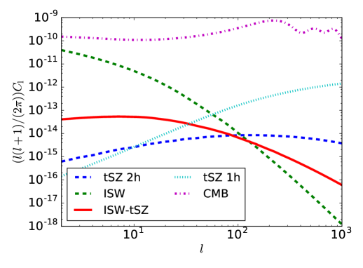
Figure 1: The ISW power spectrum $C_{l}^{\rm isw}$ (green) and the two-halo contribution ($y,2h$) to $C_{l}^{yy}$ (blue) are shown in dashed lines, while $C_{l}^{yT}$ is shown in solid red. The one-halo contribution ($y,1h$) to $C_{l}^{yy}$ is dotted. The CMB power spectrum is shown dot-dashed for comparison.

II.4 Numerical results and approximations

Fig. 1 shows the resulting power spectra. For our numerical results, we use a vacuum-energy density (in units of critical) $\Omega_{\Lambda}=0.721$, matter density $\Omega_{m}=0.279$, baryon density $\Omega_{b}=0.046$, a critical density for collapse of $\delta_{c}=1.686$, and dimensionless Hubble parameter $h=0.701$, although the large-angle results that will be our primary focus are largely insensitive to these details. In practice, we find that over ninety percent of the contribution comes from the redshift range $z=0-3$ and the halo mass range $10^{13}\,M_{\odot}$ and $10^{15}\,M_{\odot}$. We therefore integrate over slightly wider ranges; $z=0.02-4$ and halo mass $10^{12}\,M_{\odot}$ and $10^{16}\,M_{\odot}$.

The large angle (low-$l$) behaviors of the ISW-ISW autocorrelation, the $yT$ cross-correlation, and the one- and two-halo contributions to the $yy$ power spectra are easy to understand qualitatively. Let us begin with the ISW effect. Here, the $l$ dependence of the transfer function is $\Delta^{\rm isw}_{l}\propto l^{-2}$, and for large angles ($l\lesssim 20$), the power spectrum is $P(l/r)\propto l$, assuming $l+1/2\approx l$. As a result, $l^{2}C_{l}^{\rm isw}\propto l^{-1}$ for $l\lesssim 20$. Next consider the tSZ power spectra. Galaxy clusters subtend a broad distribution of angular sizes but are rarely wider than a degree. Thus, for $l\lesssim 20$, they are effectively point sources. The Fourier transform is thus effectively approximated by $y_{l}(M,z)\simeq y_{l=0}(M,z)$ which is itself precisely the integral of the $y$-distortion over the cluster image on the sky, or equivalently, the total contribution of the cluster to the angle-averaged $y$. As a result of the independence of $y_{l}$ on $l$ and $P(l/r)\propto l$ for $l\lesssim 20$, we infer $l^{2}C_{l}^{yy,2h}\propto l$ and $l^{2}C_{l}^{yT}\propto$ const for $l\lesssim 20$. Finally, the one-halo contribution to $C_{l}^{yy}$ is nearly constant (i.e., $l^{2}C_{l}\propto l^{2}$) for $l\lesssim 20$ as expected for Poisson fluctuations in what are (at these angular scales) effectively point sources.

III SZ redshift distribution

We now discuss the prospects to learn about the redshift distribution of the galaxy clusters that produce the Compton-$y$ distortion. As seen above, the $yT$ correlation is significant primarily at multipole moments $l\lesssim 100$, where the window function $y_{l}(z)$ is largely independent of $l$. The amplitude of the cross-correlation, relative to the auto-correlations, can be largely understood by examining the overlap between the redshift dependences of the two transfer functions $\Delta_{l}^{y}(z)$ and $\Delta_{l}^{\rm isw}(z)$. These transfer functions are shown in Fig. 2. More precisely, we plot–noting that $P(l/r)\propto l/r$ for the relevant angular scales—$\Delta_{l}/\left[H(z)r(z)\right]^{1/2}$, the square root of the integrands for $C_{l}$, as it is the overlap of these two functions that determines the strength of the cross-correlation relative to the auto-correlation. We also normalize the curves in Fig. 2 to both have the same area under the curve.

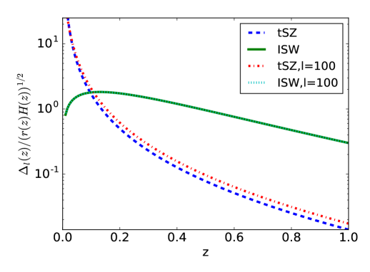
Figure 2: We plot the transfer functions $\Delta_{l}^{\rm isw}(z)$ and $\Delta_{l}^{y}(z)$, divided by $[r(z)H(z)]^{1/2}$, at $l=20$. The squares of the plotted quantities are the redshift ($z$) integrands for the ISW power spectrum $C_{l}^{\rm isw}$ and the two-halo contribution to the tSZ power spectrum $C_{l}^{yy}$. Both curves are normalized so that the areas under the curve are the same. The tSZ-ISW cross-correlation $C_{l}^{yT}$ is obtained from the overlap of these two.

Given the current fairly precise constraints to dark-energy parameters, the predictions for $\Delta_{l}^{\rm isw}(z)$ has relatively small uncertainties. The prediction for $\Delta_{l}^{y}(z)$ depends, however, on the redshift distribution of the halo mass function, bias parameters, and cluster pressure profiles, all of which involve quite uncertain physics. Measurement of the $yT$ correlation will, however, provide an additional empirical constraint on the redshift evolution of the $y$ parameter.

To see how this might work, we replace

$$\Delta_{l}^{y}(z)\to\Delta_{l}^{y}(z)\left[1+\epsilon(z-z_{0})\right],$$ (13)

where

$$z_{0}=\frac{\int\frac{dz}{r(z)H(z)}z\Delta_{l}^{y}(z)}{\int\frac{dz}{r(z)H(z)}\Delta_{l}^{y}(z)}\simeq 0.04\left(\frac{l}{100}\right).$$ (14)

The functional form in Eq. (13), is chosen so that, with $z_{0}$ given in Eq. (14), the auto-correlation power spectrum $C_{l}^{yy}$ will remain unaltered for small $\epsilon$. This alteration thus describes, for $\epsilon>0$, a weighting of the Compton-$y$ distribution to smaller redshifts (and vice versa for $\epsilon<0$) in such a way that leaves the total $y$ signal unchanged.

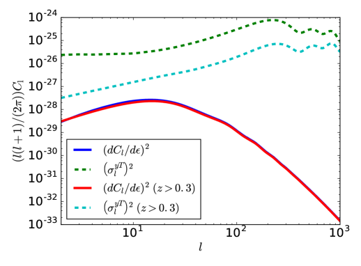
Figure 3: The derivative $\partial C_{l}^{yT}/\partial\epsilon$ of the ISW-tSZ cross-correlation with respect to $\epsilon$ (solid blue), and the ISW-tSZ noise $\sigma_{l}^{yT}$ (dashed green). We also show the same quantities restricting to $z>0.3$ (solid red and dashed cyan, respectively), which substantially increases the signal-to-noise.

We now estimate the smallest value $\sigma_{\epsilon}$ of $\epsilon$ that will be detectable with future measurements. This is given by

$$\frac{1}{\sigma_{\epsilon}^{2}}\simeq\sum_{l}\frac{\left(\partial C_{l}^{yT}/\partial\epsilon\right)^{2}}{\left(\sigma_{l}^{yT}\right)^{2}},$$ (15)

where

$$\frac{\partial C_{l}^{yT}}{\partial\epsilon}=\int\frac{c\,dz}{H(z)}\Delta^{\rm isw}_{l}(z)\Delta^{y}_{l}(z)(z-z_{0})P(l/r).$$ (16)

Fig. 3 shows $\partial C_{l}^{yT}/\partial\epsilon$ and $\sigma_{l}^{yT}$.

The error with which each $C_{l}^{yT}$ can be determined is

$$\left(\sigma_{l}^{yT}\right)^{2}=\frac{1}{2l+1}\left[\left(C_{l}^{yT}\right)^{2}+C_{l}^{TT}\left(C_{l}^{yy}+N_{l}W_{l}^{-2}\right)\right],$$ (17)

where $C_{l}^{TT}$ is the CMB temperature power spectrum, $W_{l}=e^{-l^{2}\sigma_{b}^{2}/2}$ is a window function, and $N_{l}=(4\pi/N)\sigma_{y}^{2}$ is the noise in the measurement of $C_{l}^{yy}$. Here, $\sigma_{b}$ the beam size and, $\sigma_{y}$ the root-variance of the $y$-distortion measurement in each pixel, and $N$ the number of pixels.

The Planck satellite has now measured the tSZ power spectrum and found good agreement with the expectations from the one-halo contribution to $C_{l}^{yy}$. They have now even presented good evidence for detection of the two-halo contribution at $l\lesssim 10$. From this we infer that the noise contribution $N_{l}$ to the $yy$ measurement is already small compared with $C_{l}^{yy}$, and it will be negligible for future experiments like PIXIE or PRISM. We also note from the numerical results that $\left(C_{l}^{yT}\right)^{2}$ is small compared with $C_{l}^{yy}C_{l}^{TT}$—this makes sense given that the cross-correlation of $y$ with the ISW effect is small and further that the ISW effect provides only a small contribution to large-angle temperature fluctuations. We may thus approximate

$$\left(\sigma_{l}^{yT}\right)^{2}\simeq\frac{1}{2l+1}C_{l}^{TT}C_{l}^{yy}.$$ (18)

The smallest detectable value of $\epsilon$ evaluates to $\sigma_{\epsilon}\simeq 2.3$, for $z_{0}=0.13$. This is still a considerable uncertainty, but the signal to noise can be increased. While the majority of the cross-correlation signal is at low redshifts, the 1-halo tSZ term, which appears as noise in Eq. (17), peaks even more strongly at low redshift. Thus the lowest-redshift bins are substantially noise dominated. If we remove all information at redshifts $z<0.3$, possible by explicitly detecting resolved clusters and masking them from the tSZ map, then the noise can be considerably reduced. In this case, the smallest detectable value becomes $\sigma_{\epsilon}\simeq 0.57$, which, if achieved, would provide some valuable information on the redshift distribution of tSZ fluctuations, constraining the formation of massive clusters to the era of dark energy dominance.

We also considered the profile of Ref. Komatsu:2002wc , which produces a larger tSZ signal and thus a larger cross-correlation. However, since the 1-halo tSZ term dominates the noise, this actually slightly decreased the sensitivity. Thus our results should be largely insensitive to the electron pressure profile used.

IV Primordial Non-Gaussianity

We now review the $yT$ cross-correlation from the scale-dependent primordial non-gaussianity scenario of Ref. Emami:2015xqa . If primordial perturbations are non-gaussian, the amplitude of small-wavelength power can be modulated by long-wavelength Fourier modes of the density field. The dissipation of primordial Fourier modes with wavenumbers $k\simeq 1-50$ Mpc^-1 (which takes place at redshifts $1100\lesssim z\lesssim 5\times 10^{4}$) gives rise to primordial Compton-$y$ distortions. If there is non-gaussianity, then the angular distribution of this $y$ distortion may be correlated with the large-scale density modes that give rise, through the Sachs-Wolfe effect, to large-angle fluctuations in the CMB temperature.

The predictions for this primordial $yT$ correlation depend on the yet-unmeasured isotropic value $\left\langle y\right\rangle$ of the Compton-$y$ parameter for which we take as a canonical value $4\times 10^{-9}$. The $yy$ and $yT$ power spectra for the scenario are then,

$$l^{2}C_{l}^{yy,{\rm ng}} \simeq 5.5\times 10^{-20}\,\left(\frac{f_{\rm nl}^{y}}{200}\right)^{2}\left(\frac{\left\langle y\right\rangle}{4\times 10^{-9}}\right)^{2},$$ (19)

$$l^{2}C_{l}^{yT,{\rm ng}} \simeq 5.8\times 10^{-15}\,\left(\frac{f_{\rm nl}^{y}}{200}\right)\left(\frac{\left\langle y\right\rangle}{4\times 10^{-9}}\right).$$ (20)

Here, $f_{\rm nl}^{y}$ is the non-gaussianity parameter for squeezed bispectrum configurations in which the wavenumber of the long-wavelength mode is of the $\sim$Gpc^-1 scales of modes that contribute to the ISW effect, while the two short-wavelength modes have wavelengths $1\,{\rm Mpc}^{-1}\lesssim k\lesssim 50\,{\rm Mpc}^{-1}$ As discussed in Ref. Emami:2015xqa , there are no existing model-independent constraints on $f_{\rm nl}^{y}$.

We now estimate the detectability of the $yT$ cross-correlation from non-gaussianity, discussed in Ref. Emami:2015xqa . In that work, the late-time contribution to $C_{l}^{yy}$ and $C_{l}^{yT}$ was neglected, and the detectability of the primordial signal inferred assuming that detection of $y$ fluctuations was noise-limited. Here we re-do those estimates taking into account the late-time $yT$ correlation calculated above.

If the late-time $yT$ is somehow known precisely, the signal-to-noise with which an early-Universe $yT$ signal with power spectrum $C_{l}^{yT,{\rm ng}}$ can be distinguished from the null hypothesis is

$$\left(\frac{S}{N}\right)=\left(\sum_{l}\frac{\left(C_{l}^{yT,{\rm ng}}\right)^{2}}{(\sigma_{l}^{yT})^{2}}\right)^{1/2}.$$ (21)

Using Eq. (18) and the numerical results for $C_{l}^{yy}$, we then obtain a signal-to-noise $(S/N)\simeq(f_{\rm nl}^{y}/1065)(\left\langle y\right\rangle/4\times 10^{-9})$. This calculation differs from that of Ref. Emami:2015xqa in two respects; we have included the late-time contribution to Compton-$y$ fluctuations, which degrades the detectability $f_{\rm nl}^{y}$ by about a factor of 4, even if the late-time $yT$ correlation is assumed to be known precisely. The detectability is, moreover, limited by cosmic variance and not from measurement noise. We have included in the sum in Eq. (21) angular modes up to $l\leq 1000$; the signal-to-noise improves if the sum is extended to higher $l$.

This calculation overestimates the smallest detectable signal, as there is a theoretical uncertainty in the late-time $yT$ correlation, as discussed in Section III; it must instead be determined from the data. There is thus an additional uncertainty to the inferred value of $f_{\rm nl}^{y}$ that will arise after marginalizing over the uncertain late-time $yT$ amplitude. We thus assume that the total $yT$ power spectrum is a combination $C_{l}^{yT,{\rm tot}}=\alpha C_{l}^{yT}+C_{l}^{yT,{\rm ng}}$ of the late-time and non-gaussian contributions. Here $\alpha\sim 1$ accounts for uncertainty in the amplitude of $yT$. We then calculate the Fisher matrix Jungman:1995bz ,

$$F_{ij}=\sum_{\ell}\frac{\left(\partial C_{l}^{yT,{\rm tot}}/\partial s_{i}\right)\left(\partial C_{l}^{yT,{\rm tot}}/\partial s_{j}\right)}{\left(\sigma_{l}^{yT}\right)^{2}},$$ (22)

where $\mathbf{s}=\{f_{\rm nl}^{y},\alpha\}$ is the set of parameters to be determined from the data, and the partial derivatives are evaluated under the null hypothesis $f_{\rm nl}=0$ and $\alpha=1$. The noise with which $f_{\rm nl}$ can be determined, after marginalizing over $\alpha$, is then $\left[\left(F^{-1}\right)_{f_{\rm nl}^{y}f_{\rm nl}^{y}}\right]^{1/2}$ and the signal-to-noise $(S/N)$ is $f_{\rm nl}^{y}$ divided by this quantity. Numerically, we find $(S/N)\simeq(f_{\rm nl}^{y}/1100)(\left\langle y\right\rangle/4\times 10^{-9})$. Thus, the marginalization over the ISW-tSZ effect only slightly decreases the detectability.

Since the noise is again dominated by the tSZ 1-halo term, we can perform a similar cleaning to low-redshift sources to that used in Section III. If we remove all $z<0.3$ clusters, we find that we can detect a smaller value of $f_{\rm nl}$. Numerically, using the Fisher matrix as above to marginalise over uncertainty in the $yT$ amplitude, we find $(S/N)\simeq(f_{\rm nl}^{y}/400)(\left\langle y\right\rangle/4\times 10^{-9})$, closer to the value estimated in Ref. Emami:2015xqa .

V Conclusion

Here we have calculated the tSZ-ISW cross-correlation, investigated its use in constraining the redshift distribution of $y$-parameter fluctuations, and evaluated the detectability of an early-Universe $yT$ cross-correlation. We showed that measurement of the $yT$ cross-correlation can be used to constrain the redshift distribution of the sources of $y$-parameter fluctuations, as long as low-redshift tSZ clusters can be masked, something that may be of utility given uncertainties in the cluster-physics and large-scale-structure ingredients (pressure profiles, halo biases, mass functions) that determine these fluctuations. We also showed that estimates, that neglect the $yT$ correlations induced at late times, of the detectability of early-Universe $yT$ correlations may be optimistic by factors of a few.

- (1) R. K. Sachs and A. M. Wolfe, Astrophys. J. 147, 73 (1967) [Gen. Rel. Grav. 39, 1929 (2007)].
- (2) R. A. Sunyaev and Y. B. Zeldovich, Comments Astrophys. Space Phys. 4, 173 (1972).
- (3) P. A. R. Ade et al. [Planck Collaboration], Astron. Astrophys. 571, A21 (2014) [arXiv:1303.5081 [astro-ph.CO]].
- (4) N. Aghanim et al. [Planck Collaboration], arXiv:1502.01596 [astro-ph.CO].
- (5) A. Kogut et al., JCAP 1107, 025 (2011) [arXiv:1105.2044 [astro-ph.CO]].
- (6) P. André et al. [PRISM Collaboration], JCAP 1402, 006 (2014) [arXiv:1310.1554 [astro-ph.CO]].
- (7) N. Taburet, C. Hernandez-Monteagudo, N. Aghanim, M. Douspis and R. A. Sunyaev, Mon. Not. Roy. Astron. Soc. 418, 2207 (2011) [arXiv:1012.5036 [astro-ph.CO]].
- (8) M. Lueker et al., Astrophys. J. 719, 1045 (2010) [arXiv:0912.4317 [astro-ph.CO]].
- (9) E. Komatsu et al. [WMAP Collaboration], Astrophys. J. Suppl. 192, 18 (2011) [arXiv:1001.4538 [astro-ph.CO]].
- (10) P. A. R. Ade et al. [Planck Collaboration], Astron. Astrophys. 571, A20 (2014) [arXiv:1303.5080 [astro-ph.CO]].
- (11) P. A. R. Ade et al. [Planck Collaboration], arXiv:1502.01597 [astro-ph.CO].
- (12) R. Emami, E. Dimastrogiovanni, J. Chluba and M. Kamionkowski, Phys. Rev. D 91, 123531 (2015) [arXiv:1504.00675 [astro-ph.CO]].
- (13) D. J. Fixsen, Astrophys. J. 707, 916 (2009) [arXiv:0911.1955].
- (14) E. Komatsu and T. Kitayama, Astrophys. J. 526, L1 (1999) [astro-ph/9908087].
- (15) J. M. Diego and S. Majumdar, Mon. Not. Roy. Astron. Soc. 352, 993 (2004) [astro-ph/0402449].
- (16) P. A. R. Ade et al. [Planck Collaboration], Astron. Astrophys. 581, A14 (2015) [arXiv:1502.00543 [astro-ph.CO]].
- (17) N. Itoh, Y. Kohyama and S. Nozawa, Astrophys. J. 502, 7 (1998) doi:10.1086/305876 [astro-ph/9712289].
- (18) D. Nagai, A. V. Kravtsov and A. Vikhlinin, Astrophys. J. 668, 1 (2007) doi:10.1086/521328 [astro-ph/0703661].
- (19) M. Arnaud, G. W. Pratt, R. Piffaretti, H. Boehringer, J. H. Croston and E. Pointecouteau, Astron. Astrophys. 517, A92 (2010) doi:10.1051/0004-6361/200913416 [arXiv:0910.1234 [astro-ph.CO]].
- (20) K. Dolag, E. Komatsu and R. Sunyaev, arXiv:1509.05134 [astro-ph.CO].
- (21) E. Komatsu and U. Seljak, Mon. Not. Roy. Astron. Soc. 336, 1256 (2002) [astro-ph/0205468].
- (22) J. L. Tinker et al., Astrophys. J. 688, 709 (2008) [arXiv:0803.2706 [astro-ph]].
- (23) R. K. Sheth and G. Tormen, Mon. Not. Roy. Astron. Soc. 308, 119 (1999) [astro-ph/9901122].
- (24) G. Jungman, M. Kamionkowski, A. Kosowsky and D. N. Spergel, Phys. Rev. D 54, 1332 (1996) doi:10.1103/PhysRevD.54.1332 [astro-ph/9512139].