Limits on Entanglement Effects in the String Landscape from Planck and BICEP/Keck Data

Abstract

We consider observational limits on a proposed model of the string landscape in inflation. In this scenario, effects from the decoherence of entangled quantum states in long-wavelength modes in the universe result in modifications to the Friedmann Equation and a corresponding modification to inflationary dynamics. Previous work [1, 2] suggested that such effects could provide an explanation for well-known anomalies in the Cosmic Microwave Background (CMB), such as the lack of power on large scales and the “cold spot” seen by both the WMAP and Planck satellites. In this paper, we compute limits on these entanglement effects from the Planck CMB data combined with the BICEP/Keck polarization measurement, and find no evidence for observable modulations to the power spectrum from landscape entanglement, and no sourcing of observable CMB anomalies. The originally proposed model with an exponential potential is ruled out to high significance. Assuming a Starobinsky-type $R^{2}$ inflation model, which is consistent with CMB constraints, data place a $2\sigma$ lower bound of $b>6.46\times 10^{7}\ {\rm GeV}$ on the Supersymmetry breaking scale associated with entanglement corrections.

1 Introduction

The so-called “landscape” of string theory [3, 4, 5, 6, 7, 8, 9, 10] remains an intriguing possibility. In the landscape picture, flux compactification results in a discrete collection of a large number of metastable vacua [3], each of which contains independent values of fundamental constants such as the vacuum energy, particle couplings, and Supersymmetry (SUSY) breaking scale. Inflation within these distinct vacua results in a “multiverse” of independent universes, each separated from the other by distances large compared to the Hubble length in any one region. Models for inflation in the landscape are numerous [11, 12, 13]. Despite its appeal from the perspective of fundamental theory, meaningful observational test of the string landscape has remained elusive. Efforts to connect the landscape to observables range from Anthropic arguments [14, 15, 16, 17, 18] to the possibility of bubble collisions between different landscape vacua [19, 20, 21, 22, 23, 24, 25, 26, 27], and potential trans-Planckian effects in inflation [28, 29, 30, 31]. Thus far, no solid evidence for the existence of the string landscape has been discovered.

One possible mechanism for finding observational effects of the landscape was proposed by Holman, Mersini-Houghton, and Takahashi [1, 2]. Using a mini-superspace approach, they constructed a model of the string landscape as a disordered lattice exhibiting Anderson localization [32, 33]. Localized wavepackets in different landscape vacua exhibit interference on super-Hubble length scales, resulting in nonlocal entanglement between different string vacua. Tracing over superhorizon modes [34, 35, 36] results in a locally modified Friedmann Equation

$$H^{2}=\frac{1}{3M_{\rm P}^{2}}\left(\rho+\Delta E_{\phi}\right),$$ (1.1)

where the correction $\Delta E_{\phi}$ contains the effects of the traced-over superhorizon modes. Here $M_{\rm P}\equiv m_{\rm Pl}/\sqrt{8\pi}=2.4357\times 10^{18}\ {\rm GeV}$ is the reduced Planck mass, and we take a flat Friedmann-Robertson-walker metric

$$ds^{2}=dt^{2}-a^{2}(t)d{\bf x}^{2}$$ (1.2)

and $H=\dot{a}/a$ is the Hubble parameter. This backreaction of long-wavelength modes on the local horizon can result in observable effects.

In this paper we compare the claimed predictions of this landscape entanglement model with recent Cosmic Microwave Background (CMB) data, in particular the Planck 2015 temperature and polarization spectra [37, 38, 39], and the Bicep/Keck 2014 combined data [40]. The paper is organized as follows: Section 2 discusses the specific class of landscape models tested. Section 3 presents methodology and results. Section 4 presents a summary and conclusions.

2 Landscape Entanglement Effects in Single-Field Inflation

Our approach is phenomenological. To situate landscape entanglement effects in the context of a definite model, we consider single-field inflation, which is an excellent fit to current data [30, 41, 42]. We assume a scalar field $\phi$ with a canonical Lagrangian,

$${\mathcal{L}}=\frac{1}{2}g^{\mu\nu}\partial_{\mu}\phi\partial_{\nu}\phi-V\left(\phi\right),$$ (2.1)

where the potential $V\left(\phi\right)$ is a model-dependent function: we consider two examples in this paper, first an exponential potential (Sec. 3.1),

$$V\left(\phi\right)=V_{0}e^{\lambda\phi/M_{\rm P}},$$ (2.2)

and a potential motivated by Starobinsky $R^{2}$ inflation (Sec. 3.2),

$$V\left(\phi\right)=V_{0}\left(1-e^{\sqrt{2/3}\phi/M_{\rm P}}\right)^{2}.$$ (2.3)

The energy density and pressure of a homogeneous scalar field are of the perfect fluid form, with

$$\rho = \frac{1}{2}\dot{\phi}^{2}+V\left(\phi\right),$$ (2.4)

$$p = \frac{1}{2}\dot{\phi}^{2}-V\left(\phi\right).$$ (2.5)

For a “slowly rolling” scalar field, $(1/2)\dot{\phi}^{2}\ll V\left(\phi\right)$, the field exhibits a vacuum-like equation of state, $p\simeq-\rho$, supporting accelerated expansion. The Friedmann equation for the field in the absence of entanglement modifications is

$$H^{2}=\frac{1}{3M_{\rm P}^{2}}V\left(\phi\right).$$ (2.6)

Entanglement corrections will then introduce a field-dependent modification to the potential,

$$H^{2}=\frac{1}{3M_{\rm P}^{2}}\left[V\left(\phi\right)+\delta V\left(\phi\right)\right]\equiv\frac{1}{3M_{\rm P}^{2}}V_{\rm eff}\left(\phi\right).$$ (2.7)

Following [1, 2], introducing entanglement corrections results in an effective potential of the form

$$V_{\rm eff}\left(\phi\right)=V\left(\phi\right)+\frac{1}{2}\left(\frac{V\left(\phi\right)}{3M_{\rm P}^{2}}\right)^{2}\left|F\left(\phi\right)\right|,$$ (2.8)

where

$$F\left(\phi\right)= \frac{3}{2}\left(2+\frac{m^{2}M_{\rm P}^{2}}{V\left(\phi\right)}\right)\ln\left(\frac{3b^{2}M_{\rm P}^{2}}{V\left(\phi\right)}\right)$$ (2.10)

$$-\frac{1}{2}\left(1+\frac{m^{2}}{b^{2}}\right)\exp\left(-3\frac{b^{2}M_{\rm P}^{2}}{V\left(\phi\right)}\right).$$

Here $m^{2}=V^{\prime\prime}\left(\phi\right)$ is the scalar field mass, and $b$ is a SUSY-breaking scale associated with the landscape effects, with these effects being suppressed in the limit of high scale, $b\gg 10^{10}\ {\rm GeV}$. Once the underlying inflationary potential is specified, the entanglement corrections can be calculated as a function of the additional parameter $b$ and can be compared with data. The entanglement correction (2.10) is in fact logarithmically divergent in the limit $b\rightarrow\infty$, which is an artifact of the infrared cutoff on the entanglement scale (see Ref. [1]). The correction should therefore be treated as an effective term, valid only for a limited range of scale. In practice, the logarithmic divergence does not effect constraints on the theory from data.

Previous work suggested a number of measurable effects from the presence of landscape entanglement corrections to the inflationary potential:

• Suppression of the power spectrum at large angular scales, consistent with the “Axis of Evil” [43, 44] observed in WMAP data at multipoles $\ell\leq 10$ [2].

• Running of the scalar spectral index $n_{\rm S}$ [2].

• A suppression of fluctuations due to a discontinuity in the effective potential at a scale determined by the characteristic interference length of the landscape corrections, estimated to be at a wavenumber of $k=20h\ {\rm Mpc^{-1}}$, corresponding to a scale of around $200\ {\rm Mpc}$ at a redshift $z\sim 1$ [2]. This would result in cosmic voids consistent with the observed “cold spot” in the WMAP data [45, 46].

• Anomalous cosmic “bulk flow” [47], which was suggested by analyses of the kinetic Sunyaev-Zeldovich effect in the WMAP data [48, 49, 50, 51].

• A suppression of the matter power spectrum, resulting in a value about 20-30% below the value for a $\Lambda$CDM cosmological model.

In this paper, we apply recent CMB data from the Planck satellite and the BICEP/Keck telescopes to obtain limits on power-spectrum effects from landscape entanglement, in particular:

• Suppression of power at large angular scale.

• Running of the scalar spectral index.

• Features in the power spectrum consistent with the existence of anomalous structures such as the WMAP/Planck cold spot.

• Suppressed $\sigma_{8}$ relative to $\Lambda$CDM cosmology.

The latest data strongly constrain scale-dependent modulations of the power spectrum, and we find that the primordial power spectra, including entanglement corrections during inflation, are constrained to be extremely close to a corresponding best-fit $\Lambda$CDM cosmology. We find no evidence for observably large entanglement corrections in the Planck/BICEP/Keck primordial power spectra, and we obtain a strong lower-bound on the SUSY-breaking scale $b$ for all models considered.

3 Methodology and Results

In this section, we describe the methodology used for constraining landscape entanglement effects on the power spectrum using CMB data. To enable a definite calculation, it is necessary to specify the underlying inflationary potential $V\left(\phi\right)$, since different potentials make different predictions for CMB observables [52, 53]. Single-field inflation predicts approximately power-law spectra $P_{\zeta}$ for curvature perturbations, and $P_{\rm T}$ for tensor perturbations on observable scales,

$$P_{\zeta}\left(k\right)\propto k^{n_{\rm S}-1},$$ (3.1)

and

$$P_{\rm T}\left(k\right)\propto k^{n_{T}}.$$ (3.2)

(See, e.g., Ref. [54] for a review. See also Refs. [55, 56] for a discussion of the general predictions of slow-roll inflation.) Both spectra are potential-dependent. It is conventional to describe the parameter space of inflationary observables by the scalar spectral index $n_{\rm S}$ and tensor/scalar ratio $r$, defined as the ratio of the perturbation spectra evaluated at a pivot scale $k=k_{*}$,

$$r\equiv\frac{P_{\rm T}}{P_{\zeta}}\bigg{|}_{k=k_{*}}.$$ (3.3)

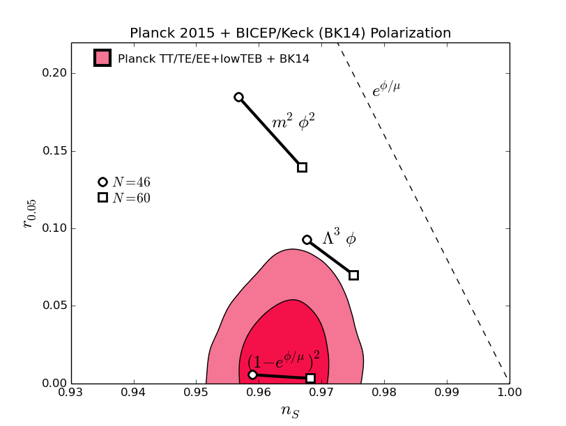
Different choices of single-field potential can then be compared to constraints from CMB data plotted in the $(n,r)$ plane. Figure 1 shows a few representative inflation models, compared with the constraints from the Planck 2015 TT/TE/EE+lowTEB temperature and polarization data [37, 38, 39], and the Bicep/Keck 2014 combined polarization data [40].

Figure 1: Planck + BKP limits on inflationary models in the parameter space of scalar spectral index $n_{\rm S}$ and tensor/scalar ratio $r$, including the models considered in this paper. The pivot scale is taken to be $k_{*}=0.05\ {\rm h\ Mpc}^{-1}$.

The allowed contours are calculated numerically using a Markov Chain Monte Carlo method with the cosmomc software package [57]. For the fiducial best-fit inflation model, we vary the following background cosmological parameters, for a total fit to eight cosmological parameters:

• Baryon density $\Omega_{\rm b}h^{2}$.

• Dark matter density $\Omega_{\rm C}h^{2}$.

• Angular scale of acoustic horizon $\theta$.

• Reionization optical depth $\tau$.

• Hubble parameter $H_{0}$.

• Power spectrum normalization $A_{s}$.

• Tensor/scalar ratio $r$.

• Scalar spectral index $n_{\rm S}$.

Curvature $\Omega_{\rm k}$ is set to zero, and the Dark Energy equation of state is fixed at $w=-1$. We fix the number of neutrino species at $N_{\nu}=3.046$, with one massive neutrino with mass $m_{\nu}=0.06\ {\rm eV}$. For these constraints, we run 8 parallel chains with Metropolis-Hastings sampling, and use a convergence criterion of the Gelman and Ruben $R$ parameter of $R-1<0.1$. The best-fit model from this set of parameters had a log likelihood of $-\ln({\mathcal{L}})=6794.396$: best-fit parameters are listed in Appendix (A). Goodness of fit of models including entanglement corrections are computed relative to this fiducial model, which we label ‘$\Lambda$CDM+r’. In Sec. (3.1), we consider the exponential model used in Ref. [2]. In Sec. (3.2), we consider entanglement corrections to a Starobinsky $R^{2}$ model.

3.1 Exponential Potential

We first consider the case of an exponential potential, which was the case considered in Ref. [2]. We take a base inflationary potential

$$V\left(\phi\right)=V_{0}\exp\left(-\frac{\lambda\phi}{M_{\rm P}}\right).$$ (3.4)

Such a potential is useful because of its analytic simplicity, allowing for exact solutions to the equations for both background dynamics and perturbations. As such, it is a useful test case. However, it has a number of shortcomings from a theoretical perspective: such potentials are not generic to Supergravity (SUGRA) scenarios, although they can be realized in special cases (see for example Ref. [58]). In addition the model lacks a graceful exit from inflation, and the unmodified potential is a poor fit to the Planck data due to overproduction of tensor perturbations. We include the model here for continuity with Refs. [1, 2]. The slow roll parameters are given by

$$\epsilon=\frac{M_{\rm P}}{2}\left(\frac{V^{\prime}}{V}\right)^{2}=\frac{\lambda^{2}}{2},$$ (3.5)

and

$$\eta=M_{\rm P}^{2}\left[\frac{V^{\prime\prime}}{V}-\frac{1}{2}\left(\frac{V^{\prime}}{V}\right)^{2}\right]=\epsilon=\frac{\lambda^{2}}{2}.$$ (3.6)

The curvature power spectrum is then a pure power-law,

$$P_{\zeta}\left(k\right)=P_{*}\left(\frac{k}{k_{*}}\right)^{n_{\rm S}-1},$$ (3.7)

with

$$n_{\rm S}-1=2\eta-4\epsilon=-\lambda^{2}.$$ (3.8)

Since $\epsilon$ is exactly constant, inflation continues forever in the absence of any new physics at some field value, and we are therefore free to fix $\phi=0$ at the times when perturbations of wavelength $k=k_{*}=0.002\ h^{-1}\ {\rm MpC}$ exited the horizon, with Planck normalization setting $P_{*}=2.2\times 10^{9}$ [38]. We can then write the power spectrum as a function of field value,

$$P_{\zeta}\left[\phi\left(k\right)\right]=\frac{1}{24\pi^{2}M_{\rm P}^{6}}\frac{V\left[\phi\left(k\right)\right]^{3}}{V^{\prime}\left[\phi\left(k\right)\right]^{2}},$$ (3.9)

where the prime is a derivative with respect to the field $\phi$, and $\phi\left(k\right)$ is defined as the field value at the time a wavenumber $k$ exited the horizon during inflation. This is straightforward to calculate using

$$dN=-d\ln(k)=-\frac{1}{M_{\rm P}\sqrt{2}}\frac{d\phi}{\sqrt{\epsilon}}=-\frac{d\phi}{\lambda M_{\rm P}}.$$ (3.10)

Here

$$N\equiv-\int{Hdt}$$ (3.11)

is the number of e-folds of expansion. Then

$$\phi_{0}\left(k\right)=\lambda M_{\rm P}\ln\left(k/k_{*}\right).$$ (3.12)

Inserting this expression into Eq. (3.9) gives an exact power-law,

$$P_{\zeta}\left(k\right)=\frac{V_{0}}{24\pi^{2}\lambda^{2}M_{\rm P}^{4}}\left(\frac{k}{k_{*}}\right)^{-\lambda^{2}}.$$ (3.13)

Therefore the Planck normalization

$$P_{*}=\frac{V_{0}}{24\pi^{2}\lambda^{2}M_{\rm P}^{4}}=2.2\times 10^{-9}$$ (3.14)

gives a constraint on the scale $V_{0}$ of inflation,

$$V_{0}=\left(5.2\times 10^{-7}\right)\left(1-n_{\rm S}\right)M_{\rm P}^{4}.$$ (3.15)

For the Planck best-fit of $1-n_{\rm S}=0.04$, this gives

$$V_{0}=2.08\times 10^{-8}\ M_{\rm P}.$$ (3.16)

Exponential potentials also predict substantial tensor production, with

$$P_{\rm T}\left(k\right)=\frac{V\left[\phi\left(k\right)\right]}{3\pi^{2}M_{\rm P}^{4}}.$$ (3.17)

The ratio $r$ of tensor to scalar power spectra is then

$$r\equiv\frac{P_{T}\left(k_{*}\right)}{P_{\zeta}\left(k_{*}\right)}=16\epsilon=8\lambda^{2}=8\left(1-n_{\rm S}\right).$$ (3.18)

For $1-n_{\rm S}=0.04$, this gives $r=0.32$, which is far higher than the $2\sigma$ upper bound of $r<0.07$ from Planck TT/TE/EE+lowTEB and BICEP/Keck. Therefore an unmodified exponential potential is inconsistent with CMB data. However, the possibility remains that entanglement corrections may lower the tensor/scalar ratio sufficiently to bring it into agreement with data.

We consider a modification to the potential of the form (2.8,2.10),

$$V_{\rm eff}\left(\phi\right)=V\left(\phi\right)+f\left[V\left(\phi\right)\right],$$ (3.19)

where $V\left(\phi\right)$ is the original potential (3.4). In general, the modification $f$ depends not only on $V$, but also on $m^{2}\left(\phi\right)=V^{\prime\prime}\left(\phi\right)$. Here we approximate the field mass as constant, $m^{2}\simeq{\rm const.}=V^{\prime\prime}\left(\phi_{0}\right)$, which is a good approximation as long as the field is slowly varying. Then we have

$$V_{\rm eff}^{\prime}\left(\phi\right)=V^{\prime}\left(\phi\right)\left[1+\frac{df}{dV}\right].$$ (3.20)

Then we have

$$d\ln(k) = \frac{1}{M_{\rm P}\sqrt{2}}\frac{d\phi}{\sqrt{\epsilon_{\rm eff}}}=\frac{1}{M_{\rm P}\sqrt{2}}\frac{d\phi}{\sqrt{\epsilon}}\left(\frac{1+f/V}{1+df/dV}\right)$$ (3.21)

$$\simeq \frac{1}{M_{\rm P}\sqrt{2}}\frac{d\phi}{\sqrt{\epsilon}}\frac{V_{\rm eff}}{V},$$ (3.22)

which is a good approximation for $f$ slowly varying. The field value as a function of wavenumber for the effective potential is then approximately [2]

$$\phi(k)\simeq\lambda M_{\rm P}\ln\left(k/k_{*}\right)\left(\frac{V\left[\phi_{0}\left(k\right)\right]}{V_{\rm eff}\left[\phi_{0}\left(k\right)\right]}\right).$$ (3.23)

The power spectrum (3.9) can then be calculated as a function of wavenumber $k$ by evaluating the effective potential (2.8) and its derivative at $\phi_{0}\left(k\right)$ given by Eq. (3.23). We accomplish this numerically via a modified version of the CAMB software (Version: January 2015) [59], with the standard power spectrum code replaced with a direct calculation using the effective potential parameters $V_{0}$, $\lambda$, and $b$. We constrain these parameters using a Markov Chain Monte Carlo (MCMC) method, as described in Sec. 3, with the parameters $n_{\rm S}$ and $r$ replaced by $V_{0}$, $\lambda$, and $b$, for a total fit to nine cosmological parameters. Sampling in the parameter in $b$ is logarithmic: i.e., the parameter directly fit by the MCMC is $\log_{10}(b)$. The tensor power spectrum is also calculated. For each case, we run 16 parallel chains with Metropolis-Hastings sampling, and use a convergence criterion of the Gelman and Ruben $R$ parameter of $R-1<0.15$.

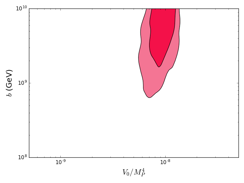
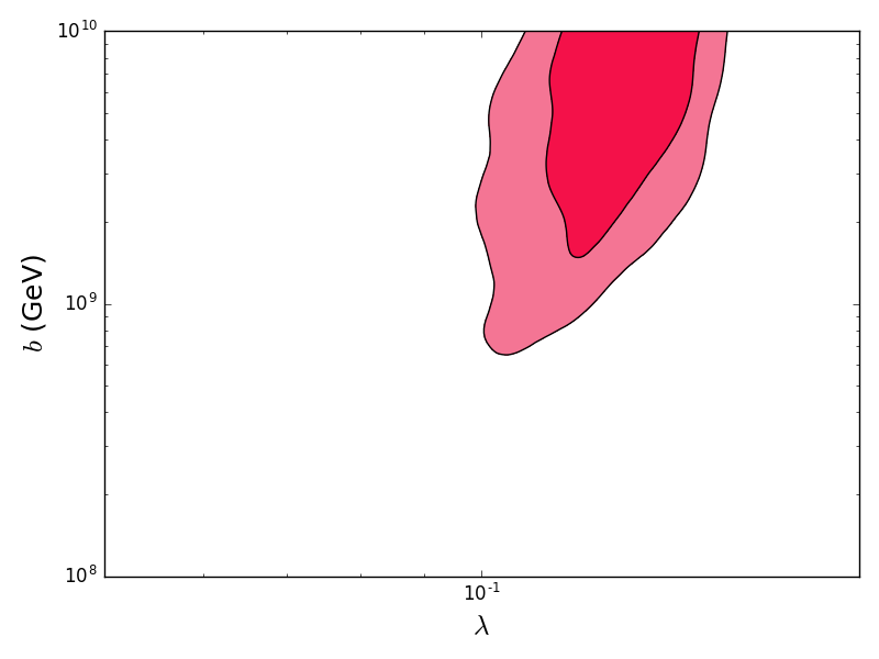
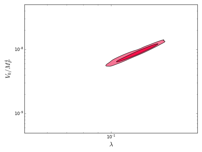
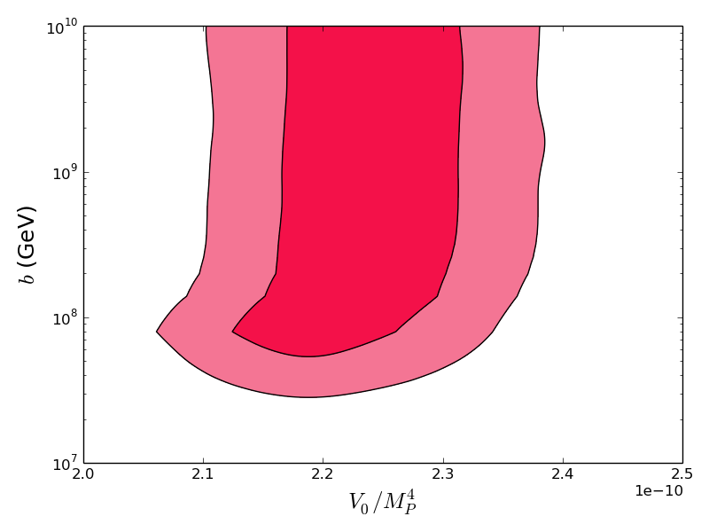
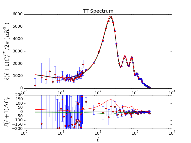
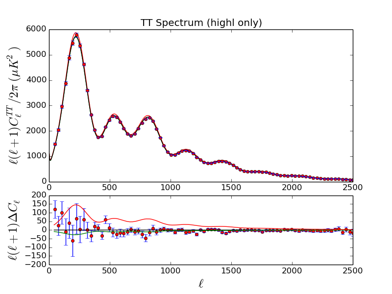
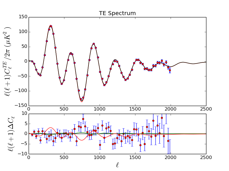
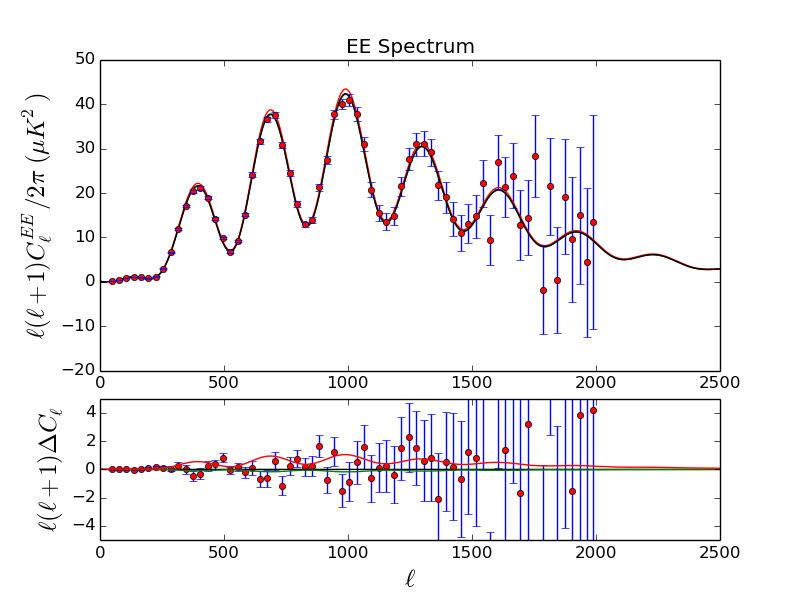
Figure 2 shows constraints on the potential parameters $V_{0}$, $\lambda$, and $b$. We obtain a lower-bound on the SUSY breaking scale $b$ of $b>1.32\times 10^{9}\ {\rm GeV}$. The overall fit of the model to the data is poor, with a best-fit log likelihood of $-\ln{\mathcal{L}}=6807.6640$, compared with $-\ln{\mathcal{L}}=6794.396$ for the $\Lambda$CDM+r model. Figure (3) shows the CMB angular power spectra for the $\Lambda$CDM+r model, and the best-fit exponential model. We conclude that the exponential potential, even with entanglement corrections, is inconsistent with data.

Figure 2: Planck limits on the parameters $V_{0}$, $b$, and $\lambda$ for the Exponential potential. Contours are for 68% and 95% confidence limits. These best-fit regions should not be considered allowed regions, as all are a poor statistical fit to Planck data. Plot limits represent actual ranges of parameters scanned by the MCMC.

Figure 3: CMB angular power spectra for the best-fit Exponential model (green), and the best-fit $\Lambda$CDM+r model (black). Points with error bars are the Planck 2015 data. Bottom pane in each plot shows residuals relative to the $\Lambda$CDM+r best-fit. This can be compared to Fig. 1 of Ref. [2]

.

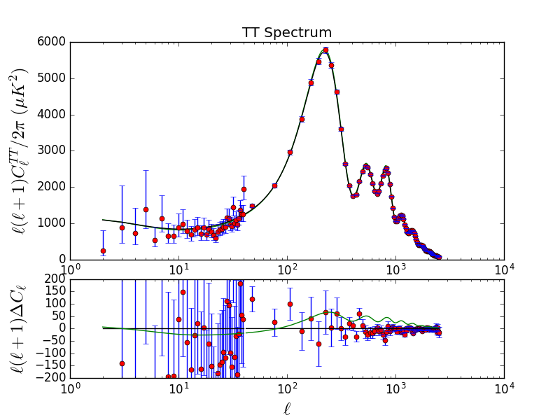
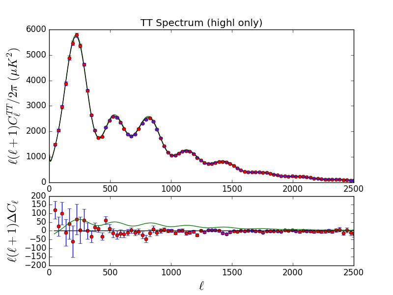
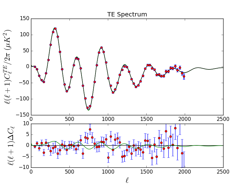
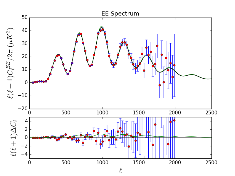
3.2 Starobinsky Potential

In this section, we consider a model which is in good agreement with existing data, and place limits on the magnitude of entanglement corrections. For this purpose, we choose the Starobinsky $R^{2}$ model [60, 61]. Despite its fundamental formulation as a modified-gravity theory, Starobinsky inflation can be re-cast in Einstein frame as an effective single-field inflation model, with potential

$$V\left(\phi\right)=V_{0}\left[1-e^{-\phi/\mu}\right]^{2},$$ (3.24)

where the mass scale $\mu$ is not a free parameter, but is fixed to be

$$\mu=\sqrt{\frac{2}{3}}M_{\rm P}.$$ (3.25)

Starobinsky-type inflation has been embedded into SUGRA scenarios in several recent works [62, 63, 64, 65, 66], and also appears in Higgs inflation [67]. As in Section 3.1, we wish to calculate an analytic expression for $\phi\left(k\right)$ suitable for numerical calculation of the power spectra. In the case of the Starobinsky potential, this will be approximate instead of exact.

The slow roll parameters (3.5), (3.6) are given by:

$$\epsilon=\frac{4}{3}\left(\frac{1}{e^{\phi/\mu}-1}\right)^{2},$$ (3.26)

and

$$\eta=\left(\frac{4}{3}\right)\frac{e^{-\phi/\mu}\left(2e^{-\phi/\mu}-1\right)-1}{\left(e^{-\phi/\mu}-1\right)^{2}}.$$ (3.27)

The number of e-folds is

$$dN=-d\ln(k) = -\frac{d\phi}{M_{\rm P}\sqrt{2\epsilon}}$$ (3.28)

$$= \frac{3}{4}\left(e^{\phi/\mu}-1\right)d\left(\frac{\phi}{\mu}\right).$$ (3.29)

For $\phi/\mu\gg 1$, the number of e-folds is then approximately

$$N\simeq\frac{3}{4}e^{\phi/\mu}.$$ (3.30)

We then have a lowest-order approximation for $\phi\left(k\right)$,

$$\phi_{0}\left(k\right)=\mu\ln{\left[\frac{4}{3}\left(N_{*}-\ln{\frac{k}{k_{*}}}\right)\right]},$$ (3.31)

where $N_{*}$ is the number of e-folds at the pivot scale $k=k_{*}$. For this analysis, we take $N_{*}=60$, consistent with high-scale inflation and rapid reheating. To leading order in $N_{*}$, the scalar spectral index is

$$n_{\rm S}-1\simeq-\frac{2}{N_{*}}=0.033,$$ (3.32)

and the tensor/scalar ratio is

$$r\simeq\frac{12}{N_{*}^{2}}=0.0033.$$ (3.33)

These values are consistent with constraints from Planck (Fig. 1). We incorporate the entanglement modifications as with the case of the exponential potential,

$$e^{\phi\left(k\right)/\mu}\simeq\ln{\left[\frac{4}{3}\left(N_{*}-\ln{\frac{k}{k_{*}}}\right)\right]}\left(\frac{V\left[\phi_{0}\left(k\right)\right]}{V_{\rm eff}\left[\phi_{0}\left(k\right)\right]}\right),$$ (3.34)

where the effective potential $V_{\rm eff}$ is again derived from $V\left(\phi\right)$ by Eqs. (2.8) and (2.10).

Numerical evaluation of the full slow-roll expression shows, however, that Eqs. (3.31) and (3.34) are accurate only to within about 10%, insufficient for an accurate numerical evaluation of the power spectrum. We can improve the approximation iteratively as follows: exactly solving the integral (3.28) gives

$$N=\frac{3}{4}\left(e^{x}-x\right)\bigg{|}_{\phi_{e}/\mu}^{\phi\left(N\right)/\mu},$$ (3.35)

where $\phi_{e}$ is the field value at the end of inflation, where $\epsilon\left(\phi_{e}\right)=1$, given by

$$\left(\phi_{e}/\mu\right)=1+\frac{2}{\sqrt{3}}.$$ (3.36)

The solution for $\phi\left(k\right)$ requires solution of a transcendental equation. We can approximate the solution by inserting the lowest-order solution $\phi_{0}\left(k\right)$ into the linear term above, with the result

$$\phi_{\rm eff}\left(k\right)\simeq\sqrt{\frac{3}{2}}M_{\rm P}\ln{\left[e^{\phi\left(k\right)/\mu}+\frac{\phi_{0}\left(k\right)}{\mu}+e^{\phi_{e}/\mu}-\frac{\phi_{e}}{\mu}\right]},$$ (3.37)

where $\phi\left(k\right)$ is given by Eq. (3.34), and $\phi_{0}\left(k\right)$ is given by the lowest-order approximation (3.31). This approximation is accurate at the level of $\Delta\phi/\phi\sim O(10^{-4})$, relative to a numerical solution. Primordial power spectra are calculated, as in the case of the exponential potential, using a modified version of CAMB directly implementing Eq. (3.13) for the scalar power spectrum, and Eq. (3.17) for the tensor power spectrum. Figure (4) shows the resulting constraints for the Starobinsky potential in the parameter plane $b$, $V_{0}$. We obtain a $2\sigma$ lower bound of $b>6.46\times 10^{7}\ {\rm GeV}$. We check consistency by comparing the analytic approximation for $P_{\zeta}\left(k\right)$ to an exact numerical integration of the slow roll parameters, and find agreement at the $O(0.001)$ level for points within the 95% confidence allowed region for Planck, demonstrating the consistency of the analytic approximations used in CAMB. For comparison with data, we consider two models:

1. The best-fit Starobinsky model, with $V_{0}=2.229236\times 10^{-10}M_{\rm P}^{4}$ and $b=6.99\times 10^{8}\ {\rm GeV}$.

2. An “extremal” Starobinsky model, with $V_{0}=2.229236\times 10^{-10}M_{\rm P}^{4}$ and $b=6.46\times 10^{7}\ {\rm GeV}$, just at the 95%-confidence lower bound for the parameter $b$, leaving all other cosmological parameters fixed at their best-fit values. This is a poor fit to the data (see Fig. 8), and is included as a reference to the most extreme modulation which is even marginally consistent with data.

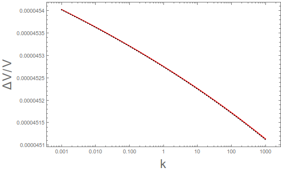
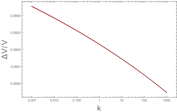
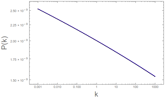
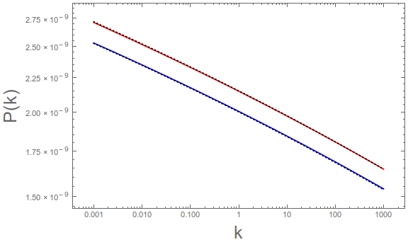
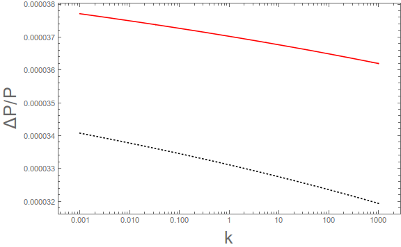
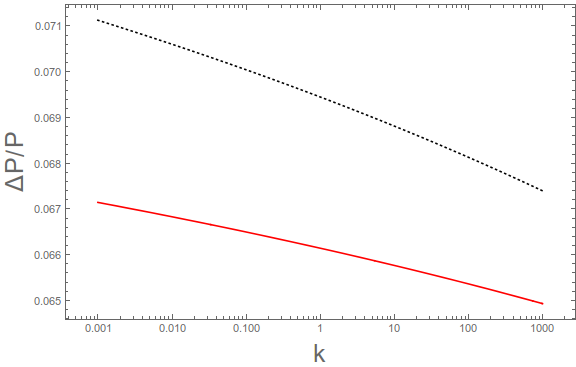
Figure (5) shows the entanglement modification $\Delta V/V$ to the potential for the best-fit and extremal models, and Figs. (6) and (7) show the corresponding power spectra and the modulation $\Delta P/P$, respectively. In the best-fit case, the power spectrum modulation is negligible, $\Delta P/P\simeq 3\times 10^{-5}$. In the extremal case, the power spectrum is of order 7%. Of particular note is the absence of any features or running in the modulated power spectrum, even in the extremal case. Nor is there suppression of power at large scales: in fact, power is slightly enhanced at large scales. In particular, we see no evidence of power suppression near the quadrupole, no running of the spectral index, and no features in the power spectrum which would explain observed CMB anomalies such as the WMAP/Planck cold spot. Figure (8) shows the CMB angular power spectra for the $\Lambda$CDM+r model, the best-fit Starobinsky model, and the extremal model.

Figure 4: Planck 68% (dark shaded) and 95% (light shaded) limits on the parameters $V_{0}$ and $b_{\rm SUSY}$ for the Starobinsky potential.

Figure 5: $\Delta V/V$ for the best-fit Starobinsky model (left), and the $2\sigma$ extremal model (right). Solid red curve is a numerical evaluation of $\phi\left(k\right)$, dotted black curve is the analytical approximation (3.37). $k$ is in units of ${\rm h\ Mpc}^{-1}$.

Figure 6: $P(k)$ for the best-fit Starobinsky model (left), and the $2\sigma$ extremal model (right). Solid red curve is the power spectrum for the entanglement-modified potential for a numerical evaluation of $\phi\left(k\right)$, and the corresponding dotted black curve is the analytical approximation (3.37). The blue curve is the unmodified power spectrum for a numerical evaluation of $\phi\left(k\right)$, and the corresponding dotted black curve is the analytical approximation. Note that in the top plot, the red curve is invisible because it is so close to the unmodified power spectrum. $k$ is in units of ${\rm h\ Mpc}^{-1}$.

Figure 7: $\Delta P(k)/P(k)$ for the best-fit Starobinsky model (left), and the $2\sigma$ extremal model (right). Solid red curve is the power spectrum for the entanglement-modified potential for a numerical evaluation of $\phi\left(k\right)$, and the corresponding dotted black curve is the analytical approximation (3.37). $k$ is in units of ${\rm h\ Mpc}^{-1}$.

Figure 8: CMB angular power spectra for the best-fit Starobinsky model (green), the extremal Starobinsky model (red), and the best-fit $\Lambda$CDM+r model (black). Points with error bars are the Planck 2015 data. Bottom pane in each plot shows residuals relative to the $\Lambda$CDM+r best-fit.

4 Conclusions

The prospect of detecting signs of stringy physics or other quantum-gravitational phenomena in high-precision cosmological data remains a tantalizing one, and new precision cosmological data are approaching the required accuracy to test stringy modifications to cosmology. In this paper, we consider one such proposed modification, relying on quantum interference effects between Anderson-localized wavepackets in a “landscape” of approximately $10^{500}$ distinct string vacua [34, 35, 36, 32, 33, 1, 2]. The authors claim a number of predictions for cosmology:

• Suppression of the power spectrum at large angular scales, consistent with the “axis of evil” [43, 44] observed in WMAP data at multipoles $\ell\leq 10$ [2].

• Running of the scalar spectral index $n_{\rm S}$ [2].

• A suppression of fluctuations due to a discontinuity in the effective potential at a scale determined by the characteristic interference length of the landscape corrections, estimated to be at a wavenumber of $k=20h\ {\rm Mpc^{-1}}$, corresponding to a scale of around $200\ {\rm Mpc}$ at a redshift $z\sim 1$ [2]. This would result in cosmic voids consistent with the observed “cold spot” in the WMAP and Planck data [45].

• Anomalous cosmic “bulk flow” [47], which was suggested by analyses of the kinetic Sunyaev-Zeldovich effect in the WMAP data [48, 49, 50, 51].

• A suppression of the matter power spectrum, resulting in $\sigma_{8}\simeq 0.8$, about 20-30% below a best-fit $\Lambda$CDM figure quoted by the authors of $\sigma_{8}=1.1$ [2]. (It is unclear where the high value for $\sigma_{8}$ was obtained, since the WMAP3 best-fit at the time was $\sigma_{8}=0.76\pm 0.05$ [68].)

A decade after the model was first proposed, new data test almost all of these claims:

• The presence of the anomalous CMB “cold spot” seen by WMAP was confirmed by Planck [69, 70], possibly associated with an anomalous void at redshift $z=0.22$ [46].

• Power suppression at the quadrupole remains in the Planck data, although the statistical significance of alignments among the lowest multipoles is debated [70, 71].

• A matter power spectrum with $\sigma_{8}\simeq 0.8$ is favored by both the WMAP data and Planck data. The Planck best-fit $\Lambda$CDM cosmology, without entanglement corrections, has $\sigma_{8}=0.830\pm 0.015$ [38].

• The presence of anomalously large bulk flow velocities has now been convincingly ruled out by a large number of independent measurements [72, 73, 74, 75, 76, 77, 78, 79, 80, 81, 82]. Current evidence strongly disfavors any model predicting large anomalous bulk flow.

In this paper, we use the Planck 2015 temperature/polarization data[37, 38, 39], and the Bicep/Keck 2014 combined data [40] to test the following claimed predictions of the landscape entanglement model:

• Suppression of power at large angular scale.

• Running of the scalar spectral index.

• Features in the power spectrum consistent with the existence of anomalous structures such as the WMAP/Planck cold spot.

• Suppressed $\sigma_{8}$ relative to $\Lambda$CDM cosmology.

We consider two cases: (1) The exponential inflationary potential proposed in the original paper [2], and (2) a Starobinsky $R^{2}$ inflation potential. Both models are compared to a fiducial $\Lambda$CDM + tensor model ($\Lambda$CDM+r) to quantify the relative likelihood of the model. Our conclusions are as follows:

• The exponential potential has three parameters: the height of the potential $V_{0}$, the coupling $\lambda$, and the SUSY-breaking scale $b$. associated with entanglement. This model is entirely ruled out by the data, with a best-fit likelihood $-\ln{({\mathcal{L}})}=6807.6640$, compared with $-\ln{({\mathcal{L}})}=6794.3960$ for the $\Lambda$CDM+r model. This is primarily because of overproduction of tensor modes, with a best-fit tensor/scalar ratio of $r=0.130768$, compared with a $\Lambda$CDM+r 95%-confidence upper bound of $r<0.06693180$. There is no evidence for observable entanglement corrections to the primordial power spectrum, with a 95%-confidence lower-bound of $b>1.12\times 10^{9}\ {\rm GeV}$, if the exponential potential is assumed as a prior.

• The Starobinsky $R^{2}$ potential has two parameters: the height of the potential $V_{0}$, and the SUSY-breaking scale $b$. The best-fit Starobinsky $R^{2}$ model, including entanglement corrections, is a good fit to data, with a best-fit $-\ln{({\mathcal{L}})}=6792.9980$. (Remarkably, even the unmodified Starobinsky potential gives a better fit to the data with fewer parameters than $\Lambda$CDM+r!) However, entanglement corrections are constrained to be unobservably small, with a 95%-confidence lower bound on the SUSY breaking scale of $b>6.46\times 10^{7}\ {\rm GeV}$. With respect to tests of predictions:

  • There is no suppression of power on large angular scales: power is in fact slightly enhanced on large scales.

  • Modulation of the power spectrum is nearly scale invariant, and no observable running of the spectral index is present. Running of the spectral index is of order $\alpha=-0.0006$, consistent with an unmodified Starobinsky $R^{2}$ potential.

  • There are no features induced in the power spectrum, so entanglement corrections do not provide the modulation which would be required to explain the WMAP/Planck cold spot.

  • We find no evidence for suppression of $\sigma_{8}$ relative to the best-fit $\Lambda$CDM+r cosmology. The best-fit $\Lambda$CDM+r cosmology used in this paper has $\sigma_{8}=0.8299$, and the best-fit Starobinsky model, including entanglement corrections, has $\sigma_{8}=0.8314$, consistent with the Planck $\Lambda$CDM favored value $\sigma_{8}=0.830\pm 0.015$ [38]. The $2\sigma$ “extremal” Starobinsky model has $\sigma_{8}=0.8439$, which is actually enhanced rather than suppressed relative to $\Lambda$CDM.

Appendix A contains a table of all parameter fits.

It is worthwhile to discuss in general the “concrete predictions” originally claimed by the authors of Refs. [1, 2], since several key claims do not survive even cursory scrutiny. For example, the discontinuity in the effective potential claimed to be correlated with voids and the CMB cold spot does not appear to in fact exist: for all physically relevant values of the parameters $V_{0}$, $\lambda$, and $b$, the modulation $F\left(\phi\right)$ is a smooth function, with no characteristic discontinuities which would explain features in the power spectrum. Perhaps more importantly, the form of the effective potential resulting from landscape entanglement is completely dependent on the choice of inflationary potential $V\left(\phi\right)$, which is itself an arbitrary free function. One could just as consistently choose the underlying inflationary potential in the absence of landscape corrections to be the same as the effective potential (2.8)! In this sense, the landscape model is no more (or less) predictive than single-field inflation itself, and most of the claimed predictions of the entanglement model turn out not to have been predictions at all. However, any considerations of theoretical consistency are a moot point: even if one takes the claimed predictions at face value, almost all of them are ruled out by Planck. Experiment always supersedes theory, and the model does not match the data.

Finally, we note that the general conclusion about constraints on modulations of the power spectrum, while derived here in the context of a specific model, is a largely model-independent statement. Modulations of the primordial power spectrum from entanglement are ruled out precisely because any observably large modulations of the primordial power spectrum will introduce substantial tension with the Planck data, relative to a pure power law [83, 84]. While it is undoubtedly possible to a posteriori engineer a modulated power spectrum which improves the fit to Planck (see, e.g. the interesting case presented in Ref. [85]), such models will necessarily require multiple tuned parameters and it is therefore questionable in such a case if even a substantially improved fit can be considered favored from a Bayesian perspective.

Appendix A Parameter Table

This section contains a table of 1-D parameter fits for the models considered in this paper. Error bars are one standard deviation, and upper/lower bounds are 95% confidence. Parameters listed in parentheses “()” are derived parameters calculated from the best-fit values for $V_{0}$, $b$, and $\lambda$. Also included is the derived best-fit running for the spectral index, $\alpha\equiv dn/d\ln{k}$. Observables are quoted at a pivot scale $k_{*}=0.05\ \mathrm{h\ Mpc}^{-1}$.

	$\Lambda$CDM+r	Exponential	Starobinsky
$\Omega_{\rm b}h^{2}$	$0.02222473\pm 0.00016$	$0.02250676\pm 0.00015$	$0.02225708\pm 0.00014$
$\Omega_{\rm c}h^{2}$	$0.1199321\pm 0.0015$	$0.1155528\pm 0.0012$	$0.1195799\pm 0.00095$
$\theta$	$1.040745\pm 0.00032$	$1.041232\pm 0.00032$	$1.040792\pm 0.00029$
$\tau$	$0.08100027\pm 0.016$	$0.1031400\pm 0.017$	$0.08644387\pm 0.015$
$H_{0}$	$67.20348\pm 0.66$	$69.1682\pm 0.55$	$67.36688\pm 0.43$
$\ln{\left(10^{10}A_{s}\right)}$	$3.097646\pm 0.031$	$(3.14846)$	$(3.10186)$
$r$	$<0.06693180$ (95%)	$(0.130768)$	$(0.0032943)$
$n_{\rm S}$	$0.9644768\pm 0.0048$	$(0.984077)$	$(0.965991)$
$\alpha$	-	$(3.6\times 10^{-6})$	$(-0.000061)$
$\sigma_{8}$	(0.8299)	(0.8360)	(0.8314)
$10^{9}V_{0}/M_{\rm P}^{4}$	-	$9.377153\pm 1.8$	$0.2229236\pm 0.0068$
$\log_{10}{b\ ({\rm GeV})}$	-	$>9.048864$ (95%)	$>7.811044$ (95%)
$\lambda$	-	$0.1261851\pm 0.012$	-
Likelihood	$6794.3960$	$6807.6640$	$6792.9980$

References

- [1] R. Holman, L. Mersini-Houghton and T. Takahashi, Cosmological avatars of the landscape I: Bracketing the SUSY breaking scale, Phys. Rev. D77 (2008) 063510, [hep-th/0611223].
- [2] R. Holman, L. Mersini-Houghton and T. Takahashi, Cosmological Avatars of the Landscape. II. CMB and LSS Signatures, Phys. Rev. D77 (2008) 063511, [hep-th/0612142].
- [3] R. Bousso and J. Polchinski, Quantization of four form fluxes and dynamical neutralization of the cosmological constant, JHEP 06 (2000) 006, [hep-th/0004134].
- [4] T. Banks, M. Dine and E. Gorbatov, Is there a string theory landscape?, JHEP 08 (2004) 058, [hep-th/0309170].
- [5] M. R. Douglas, The Statistics of string / M theory vacua, JHEP 05 (2003) 046, [hep-th/0303194].
- [6] B. Freivogel and L. Susskind, A Framework for the landscape, Phys. Rev. D70 (2004) 126007, [hep-th/0408133].
- [7] F. Denef, M. R. Douglas and B. Florea, Building a better racetrack, JHEP 06 (2004) 034, [hep-th/0404257].
- [8] M. Dine, E. Gorbatov and S. D. Thomas, Low energy supersymmetry from the landscape, JHEP 08 (2008) 098, [hep-th/0407043].
- [9] M. R. Douglas, Statistical analysis of the supersymmetry breaking scale, hep-th/0405279.
- [10] M. R. Douglas, Basic results in vacuum statistics, Comptes Rendus Physique 5 (2004) 965–977, [hep-th/0409207].
- [11] D. Baumann and L. McAllister, Advances in Inflation in String Theory, Ann. Rev. Nucl. Part. Sci. 59 (2009) 67–94, [0901.0265].
- [12] C. P. Burgess, M. Cicoli and F. Quevedo, String Inflation After Planck 2013, JCAP 1311 (2013) 003, [1306.3512].
- [13] D. Baumann and L. McAllister, Inflation and String Theory. Cambridge University Press, 2015.
- [14] J. D. Barrow and F. J. Tipler, The Anthropic Cosmological Principle. Oxford U. Pr., Oxford, 1988.
- [15] L. Susskind, The Anthropic landscape of string theory, hep-th/0302219.
- [16] S. Weinstein, Anthropic reasoning in multiverse cosmology and string theory, Class. Quant. Grav. 23 (2006) 4231–4236, [hep-th/0508006].
- [17] G. F. R. Ellis and L. Smolin, The Weak anthropic principle and the landscape of string theory, 0901.2414.
- [18] D. F. Watson, On the Anthropic Principle in the Multiverse: Addressing Provability and Tautology, 1103.6044.
- [19] J. Garriga, A. H. Guth and A. Vilenkin, Eternal inflation, bubble collisions, and the persistence of memory, Phys. Rev. D76 (2007) 123512, [hep-th/0612242].
- [20] M. P. Salem, P. Saraswat and E. Shaghoulian, Gravity waves from cosmic bubble collisions, JCAP 1302 (2013) 019, [1210.4165].
- [21] L. Mersini-Houghton and M. J Perry, The End of Eternal Inflation, Class. Quant. Grav. 31 (2014) 165005, [1211.1347].
- [22] S. Osborne, L. Senatore and K. Smith, Collisions with other Universes: the Optimal Analysis of the WMAP data, 1305.1964.
- [23] C. L. Wainwright, M. C. Johnson, H. V. Peiris, A. Aguirre, L. Lehner and S. L. Liebling, Simulating the universe(s): from cosmic bubble collisions to cosmological observables with numerical relativity, JCAP 1403 (2014) 030, [1312.1357].
- [24] C. L. Wainwright, M. C. Johnson, A. Aguirre and H. V. Peiris, Simulating the universe(s) II: phenomenology of cosmic bubble collisions in full General Relativity, JCAP 1410 (2014) 024, [1407.2950].
- [25] P. Zhang and M. C. Johnson, Testing eternal inflation with the kinetic Sunyaev Zel’dovich effect, JCAP 1506 (2015) 046, [1501.00511].
- [26] M. C. Johnson, C. L. Wainwright, A. Aguirre and H. V. Peiris, Simulating the Universe(s) III: Observables for the full bubble collision spacetime, JCAP 1607 (2016) 020, [1508.03641].
- [27] M. C. Johnson and W. Lin, Observable Signatures of a Classical Transition, JCAP 1603 (2016) 051, [1508.03786].
- [28] R. Easther, W. H. Kinney and H. Peiris, Observing trans-Planckian signatures in the cosmic microwave background, JCAP 0505 (2005) 009, [astro-ph/0412613].
- [29] P. D. Meerburg, R. Wijers and J. P. van der Schaar, WMAP 7 Constraints on Oscillations in the Primordial Power Spectrum, Mon. Not. Roy. Astron. Soc. 421 (2012) 369, [1109.5264].
- [30] Planck collaboration, P. A. R. Ade et al., Planck 2015 results. XX. Constraints on inflation, 1502.02114.
- [31] R. H. Brandenberger and J. Martin, Trans-Planckian Issues for Inflationary Cosmology, Class. Quant. Grav. 30 (2013) 113001, [1211.6753].
- [32] A. Kobakhidze and L. Mersini-Houghton, Birth of the universe from the landscape of string theory, Eur. Phys. J. C49 (2007) 869–873, [hep-th/0410213].
- [33] L. Mersini-Houghton, Can we predict Lambda for the non-SUSY sector of the landscape, Class. Quant. Grav. 22 (2005) 3481–3490, [hep-th/0504026].
- [34] J. J. Halliwell and S. W. Hawking, The Origin of Structure in the Universe, Phys. Rev. D31 (1985) 1777.
- [35] C. Kiefer, Continuous Measurement of Minisuperspace Variables by Higher Multipoles, Class. Quant. Grav. 4 (1987) 1369.
- [36] C. Kiefer, Decoherence in quantum electrodynamics and quantum gravity, Phys. Rev. D46 (1992) 1658–1670.
- [37] Planck collaboration, R. Adam et al., Planck 2015 results. I. Overview of products and scientific results, 1502.01582.
- [38] Planck collaboration, P. A. R. Ade et al., Planck 2015 results. XIII. Cosmological parameters, 1502.01589.
- [39] Planck collaboration, N. Aghanim et al., Planck 2015 results. XI. CMB power spectra, likelihoods, and robustness of parameters, Submitted to: Astron. Astrophys. (2015) , [1507.02704].
- [40] BICEP2, Keck Array collaboration, P. A. R. Ade et al., BICEP2 / Keck Array V: Measurements of B-mode Polarization at Degree Angular Scales and 150 GHz by the Keck Array, Astrophys. J. 811 (2015) 126, [1502.00643].
- [41] BICEP2, Planck collaboration, P. A. R. Ade et al., Joint Analysis of BICEP2/ and Data, Phys. Rev. Lett. 114 (2015) 101301, [1502.00612].
- [42] J. Martin, The Observational Status of Cosmic Inflation after Planck, 2015. 1502.05733.
- [43] A. de Oliveira-Costa, M. Tegmark, M. Zaldarriaga and A. Hamilton, The Significance of the largest scale CMB fluctuations in WMAP, Phys. Rev. D69 (2004) 063516, [astro-ph/0307282].
- [44] K. Land and J. Magueijo, The Axis of evil, Phys. Rev. Lett. 95 (2005) 071301, [astro-ph/0502237].
- [45] C. L. Bennett et al., Seven-Year Wilkinson Microwave Anisotropy Probe (WMAP) Observations: Are There Cosmic Microwave Background Anomalies?, Astrophys. J. Suppl. 192 (2011) 17, [1001.4758].
- [46] A. Kovács et al., Supervoid Origin of the Cold Spot in the Cosmic Microwave Background, IAU Symp. 306 (2015) 269–272, [1407.1470].
- [47] L. Mersini-Houghton and R. Holman, ’Tilting’ the Universe with the Landscape Multiverse: The ’Dark’ Flow, JCAP 0902 (2009) 006, [0810.5388].
- [48] A. Kashlinsky, F. Atrio-Barandela, D. Kocevski and H. Ebeling, A measurement of large-scale peculiar velocities of clusters of galaxies: results and cosmological implications, Astrophys. J. 686 (2009) L49–L52, [0809.3734].
- [49] R. Watkins, H. A. Feldman and M. J. Hudson, Consistently Large Cosmic Flows on Scales of 100 Mpc/h: a Challenge for the Standard LCDM Cosmology, Mon. Not. Roy. Astron. Soc. 392 (2009) 743–756, [0809.4041].
- [50] A. Kashlinsky, F. Atrio-Barandela, H. Ebeling, A. Edge and D. Kocevski, A new measurement of the bulk flow of X-ray luminous clusters of galaxies, Astrophys. J. 712 (2010) L81–L85, [0910.4958].
- [51] H. A. Feldman, R. Watkins and M. J. Hudson, Cosmic Flows on 100 Mpc/h Scales: Standardized Minimum Variance Bulk Flow, Shear and Octupole Moments, Mon. Not. Roy. Astron. Soc. 407 (2010) 2328–2338, [0911.5516].
- [52] S. Dodelson, W. H. Kinney and E. W. Kolb, Cosmic microwave background measurements can discriminate among inflation models, Phys. Rev. D56 (1997) 3207–3215, [astro-ph/9702166].
- [53] W. H. Kinney, Constraining inflation with cosmic microwave background polarization, Phys. Rev. D58 (1998) 123506, [astro-ph/9806259].
- [54] W. H. Kinney, TASI Lectures on Inflation, 0902.1529.
- [55] V. F. Mukhanov and G. V. Chibisov, Quantum Fluctuations and a Nonsingular Universe, JETP Lett. 33 (1981) 532–535.
- [56] V. F. Mukhanov, CMB, quantum fluctuations and the predictive power of inflation, astro-ph/0303077.
- [57] A. Lewis and S. Bridle, Cosmological parameters from CMB and other data: A Monte Carlo approach, Phys. Rev. D66 (2002) 103511, [astro-ph/0205436].
- [58] K. Nakayama and F. Takahashi, General Analysis of Inflation in the Jordan frame Supergravity, JCAP 1011 (2010) 039, [1009.3399].
- [59] A. Lewis, A. Challinor and A. Lasenby, Efficient computation of CMB anisotropies in closed FRW models, Astrophys. J. 538 (2000) 473–476, [astro-ph/9911177].
- [60] A. A. Starobinsky, A New Type of Isotropic Cosmological Models Without Singularity, Phys. Lett. B91 (1980) 99–102.
- [61] A. Kehagias, A. M. Dizgah and A. Riotto, Remarks on the Starobinsky model of inflation and its descendants, Phys. Rev. D89 (2014) 043527, [1312.1155].
- [62] S. V. Ketov and A. A. Starobinsky, Embedding ()-Inflation into Supergravity, Phys. Rev. D83 (2011) 063512, [1011.0240].
- [63] S. V. Ketov and A. A. Starobinsky, Inflation and non-minimal scalar-curvature coupling in gravity and supergravity, JCAP 1208 (2012) 022, [1203.0805].
- [64] S. Ferrara, R. Kallosh and A. Van Proeyen, On the Supersymmetric Completion of Gravity and Cosmology, JHEP 11 (2013) 134, [1309.4052].
- [65] S. V. Ketov, Starobinsky Model in Supergravity, Phys. Rev. D89 (2014) 085042, [1402.0626].
- [66] S. Ferrara, A. Kehagias and M. Porrati, Supergravity, JHEP 08 (2015) 001, [1506.01566].
- [67] F. L. Bezrukov and M. Shaposhnikov, The Standard Model Higgs boson as the inflaton, Phys. Lett. B659 (2008) 703–706, [0710.3755].
- [68] WMAP collaboration, D. N. Spergel et al., Wilkinson Microwave Anisotropy Probe (WMAP) three year results: implications for cosmology, Astrophys. J. Suppl. 170 (2007) 377, [astro-ph/0603449].
- [69] Planck collaboration, P. A. R. Ade et al., Planck 2015 results. XVI. Isotropy and statistics of the CMB, 1506.07135.
- [70] D. J. Schwarz, C. J. Copi, D. Huterer and G. D. Starkman, CMB Anomalies after Planck, Class. Quant. Grav. 33 (2016) 184001, [1510.07929].
- [71] A. Rassat, J. L. Starck, P. Paykari, F. Sureau and J. Bobin, Planck CMB Anomalies: Astrophysical and Cosmological Secondary Effects and the Curse of Masking, JCAP 1408 (2014) 006, [1405.1844].
- [72] R. Keisler, The Statistical Significance of the ’Dark Flow’, Astrophys. J. 707 (2009) L42–L44, [0910.4233].
- [73] S. J. Osborne, D. S. Y. Mak, S. E. Church and E. Pierpaoli, Measuring the Galaxy Cluster Bulk Flow from WMAP data, Astrophys. J. 737 (2011) 98, [1011.2781].
- [74] D.-C. Dai, W. H. Kinney and D. Stojkovic, Measuring the cosmological bulk flow using the peculiar velocities of supernovae, JCAP 1104 (2011) 015, [1102.0800].
- [75] A. Nusser and M. Davis, The cosmological bulk flow: consistency with CDM and constraints on and , Astrophys. J. 736 (2011) 93, [1101.1650].
- [76] S. J. Turnbull, M. J. Hudson, H. A. Feldman, M. Hicken, R. P. Kirshner and R. Watkins, Cosmic flows in the nearby universe from Type Ia Supernovae, Mon. Not. Roy. Astron. Soc. 420 (2012) 447–454, [1111.0631].
- [77] G. Lavaux, N. Afshordi and M. J. Hudson, First measurement of the bulk flow of nearby galaxies using the cosmic microwave background, Mon. Not. Roy. Astron. Soc. 430 (2013) 1617–1635, [1207.1721].
- [78] Planck collaboration, P. A. R. Ade et al., Planck 2013 results. XIX. The integrated Sachs-Wolfe effect, Astron. Astrophys. 571 (2014) A19, [1303.5079].
- [79] B. Rathaus, E. D. Kovetz and N. Itzhaki, Studying the Peculiar Velocity Bulk Flow in a Sparse Survey of Type-Ia SNe, Mon. Not. Roy. Astron. Soc. 431 (2013) 3678, [1301.7710].
- [80] Y.-Z. Ma and J. Pan, An estimation of local bulk flow with the maximum-likelihood method, Mon. Not. Roy. Astron. Soc. 437 (2014) 1996–2004, [1311.6888].
- [81] D. Huterer, D. L. Shafer and F. Schmidt, No evidence for bulk velocity from type Ia supernovae, JCAP 1512 (2015) 033, [1509.04708].
- [82] M. I. Scrimgeour et al., The 6dF Galaxy Survey: Bulk Flows on Mpc scales, Mon. Not. Roy. Astron. Soc. 455 (2016) 386–401, [1511.06930].
- [83] X. Chen, C. Dvorkin, Z. Huang, M. H. Namjoo and L. Verde, The Future of Primordial Features with Large-Scale Structure Surveys, 1605.09365.
- [84] X. Chen, P. D. Meerburg and M. Münchmeyer, The Future of Primordial Features with 21 cm Tomography, 1605.09364.
- [85] D. K. Hazra, A. Shafieloo, G. F. Smoot and A. A. Starobinsky, Primordial features and Planck polarization, JCAP 1609 (2016) 009, [1605.02106].