Controlling local currents in molecular junctions

Abstract

The effect of non-equilibrium constraints and dephasing on the circulating currents in molecular junctions are analyzed. Circulating currents are manifestations of quantum effects and can be induced either by externally applied bias or an external magnetic field through the molecular system. In symmetric Aharonov-Bohm ring, bond currents have two contributions, bias driven and magnetic field driven. We analyze the competition between these two contributions and show that, as a consequence, current through one of the branches can be completely suppressed. We then study the effect of asymmetry (as a result of chemical substitution) on the current pathways inside the molecule and study asymmetry induced circulating currents (without magnetic field) by tuning the coupling strength of the substituent (at finite bias).

I Introduction

Persistent charge current is the current flowing in systems with ring geometries, due to the phase coherent motion of electrons imry . It can be induced by the presence of vector potential due to magnetic fields threading the ring, first studied by Pauling in the context of aromatic molecules pauling . The effect of magnetic flux through superconducting discs was studied by Byers and Yang byers . Buttiker et.al. buttiker , showed that 1D metallic rings, where phase coherence of electrons is maintained, act like superconductors to produce a persistent current flowing in the ring. Further studies have explored the effects of various quantities like disorder, temperature and coulomb interaction between electrons on the persistent current imry . In this study we extend these works to the molecular regime in the molecular junction setup.

In recent years, the electron conduction through single molecular junction has attracted a lot of research interest due to its fundamental interest in exploring quantum effects and its applications in miniaturization of electronic components (molecular electronics). The idea of molecular electronics is to control the electronic current by manipulating the physical and chemical properties of the molecule. Current flowing through molecules in junction can take different pathways inside a molecule. These pathways have been studied recently solomon . Here we analyze the local currents inside a molecular junction in presence (in symmetric junction) and absence (asymmetric junction) of the magnetic field.

Magnetic field threading the molecular ring induces different phases in the electron wavefunction as it transverses through different pathways inside the molecule. As we discuss below, this phase acquired by the electron affects both the local currents and the net current. Hence the dependence of current flow on magnetic flux allows to control not only the net current through the junction but also the local bond currents inside the junction. Although much work has been done to study the effect of magnetic flux on current flowing between leads rai ; solomon ; Hod1 ; Hod2 , little attention has been paid to the study of the effect of magnetic flux on the circulating currents inside the molecule in the presence of external bias, with notable exceptions of references Rai1 ; Rai2 ; Jayannavar1 ; Davidovich . Here we analyze the aspect of controlling the local currents by manipulating external magnetic field and chemical substitution. For a symmetric Aharonov-Bohm ring case, in the presence of the external bias, it is possible to fine tune the magnetic flux to completely suppress current flow across different branches selectively. We show that the bond current has two contributions, which we identify as magnetic field driven and bias driven contributions. These two contributions compete and may cancel each other along a branch, while add up to enhance the current along the other branch. This is not possible if either the magnetic field or the bias is present alone. We further consider the case where an extra site is coupled to the ring system and demonstrate that a circulating current (in this work we adapt an intuitive definition of circulating current as, ”circulating current is present if the direction of current flowing through one of the branches is opposite to the direction of the net current, and its magnitude is given by the smallest of the currents flowing across the two branches”) can also be induced by tuning the coupling strength of the substituent (at finite bias). This is due to the asymmetry induced between pathways by the extra coupling site. We derive analytic expressions for the bond currents and discuss them under different conditions. We find that the circulating currents can be induced not only by the magnetic field but also due to coupling with the leads (in the presence of asymmetry and finite bias). That is the direction of the current flowing across a branch can be manipulated by tuning the coupling strength with the leads. We present a detailed analysis of bond currents based on analytical results.

The rest of the paper is organized as follows. In the next section (Sec.(II)) we consider a model with asymmetry in the presence of magnetic field and calculate the bond currents inside the molecule and the net current in the circuit. In Sec, (III), we present a symmetric molecular ring system coupled to two metal leads in the presence of a magnetic flux. We discuss bond currents, net current and the circulating current at equilibrium (when the two leads are at the same thermodynamic state) and non-equilibrium conditions. In Sec. (IV) we discuss circulating currents in an asymmetric molecular ring junction in absence of the magnetic field. We conclude in Sec. (V).

II Model Hamiltonian and Current calculations

Model Hamiltonian

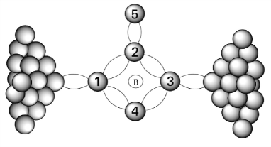
Figure 1: (Color online) Schematic of model system considered. It consists of four identical localized sites coupled to each other to form a ring geometry (with magnetic field piercing the ring), diagonally opposite sites are coupled to two metal leads and one of the sites not coupled to leads is coupled to an extra site.

To study the effect of asymmetry and magnetic fields on bond currents in ring molecular systems out of equilibrium (at steady-state), we consider a simple model shown in Fig. 1. It consists of a ring molecular system with four identical localized sites (orbitals) coupled to nearest sites through hopping. Diagonally opposite sites are coupled to two metal leads, and one of the sites not coupled to leads is coupled to an extra site. Further a magnetic flux is pierced through the molecular ring. All four sites forming the ring are taken to have the same energy (taken as zero by rescaling all other energies) and their coupling strengths to nearest neighbors are equal, taken as energy unit. Specifically, sites ’1’ $\&$ ’3’ are coupled to left and right metallic leads (modeled as free electron reservoirs at thermal equilibrium) respectively. Site ’2’ is coupled to an extra site (site ’5’ with energy ’$\epsilon$’) with coupling strength ’$t$’. Effect of the external magnetic field is included in the model Hamiltonian in the spirit of Peierls substitution peierls .

The Hamiltonian describing this model is given as,

$$\hat{H} = \sum_{i,j=1}^{5}H_{0_{ij}}c_{i}^{{\dagger}}c_{j}+\mathop{\sum_{k}}_{\alpha=L,R}\epsilon_{\alpha,k}d_{\alpha k}^{\dagger}d_{\alpha k}$$ (1)

$$+ \sum_{k}\big{[}g_{L}d_{Lk}^{\dagger}c_{1}+g_{R}d_{Rk}^{\dagger}c_{3}+h.c.\big{]}$$

where

$$H_{0}=\begin{pmatrix}0&-e^{-i\frac{\phi}{4}}&0&-e^{i\frac{\phi}{4}}&0\\ -e^{i\frac{\phi}{4}}&0&-e^{-i\frac{\phi}{4}}&0&-t\\ 0&-e^{i\frac{\phi}{4}}&0&-e^{-i\frac{\phi}{4}}&0\\ -e^{-i\frac{\phi}{4}}&0&-e^{i\frac{\phi}{4}}&0&0\\ 0&-t&0&0&\epsilon\\ \end{pmatrix}$$ (2)

is the single particle Hamiltonian for the isolated molecule. ’$\phi$’ is the dimensionless magnetic flux given by $(B\times A)/(\frac{\hbar c}{e})$, where ’B’ is the strength of applied magnetic field, ’A’ is the area of the molecular ring and $\hbar$, c, e represents reduced Planck’s constant, speed of light and (absolute) charge of an electron respectively. Here $c_{i}$ ($c_{i}^{{\dagger}}$) are the fermion annihilation (creation) operators for destroying (creating) electron at site ’$i$’ and similarly $d_{\alpha k}$ ($d_{\alpha k}^{{\dagger}}$) are operators for destroying (creating) electron in state ’k’ in the ’$\alpha$’ lead ($\alpha=L/R$). First two terms in the Hamiltonian represent free system and free lead Hamiltonians, and the third term represents hybridization between system and lead sites. We also assumed wide-band approximation (i.e., system lead hybridization is independent of ’k’).

Bond currents

Expressions for bond current operators between localized sites can be obtained from the continuity equation for charge density operator at any localized site. For example rate of change of charge at site ’1’ i.e,

$$\frac{d}{dt}(-ec_{1}^{{\dagger}}c_{1})= \frac{ie}{\hbar}[c_{1}^{{\dagger}}c_{1},H]$$ (3)

gives three terms on the R.H.S. and each of these three terms can be identified as the operator for current from site ’1’ to site ’2’ or to site ’4’ or to left lead regions. In particular, the operator for current from site ’2’ to ’1’ and from site ’4’ to ’1’can be identified as,

$$\hat{I}_{2\rightarrow 1}=\frac{ie}{\hbar}\big{(}e^{i\frac{\phi}{4}}c_{2}^{{\dagger}}c_{1}-e^{-i\frac{\phi}{4}}c_{1}^{{\dagger}}c_{2}\big{)}$$ (4)

and

$$\hat{I}_{4\rightarrow 1}=\frac{ie}{\hbar}\big{(}e^{-i\frac{\phi}{4}}c_{4}^{{\dagger}}c_{1}-e^{i\frac{\phi}{4}}c_{1}^{{\dagger}}c_{4}\big{)}$$ (5)

whose average gives the bond currents flowing between sites ’1’ $\&$ ’2’ ($I_{2\rightarrow 1}$) and ’1’ $\&$ ’4’ ($I_{4\rightarrow 1}$)). At steady state these two bond currents are expressed as,

$$I_{2\rightarrow 1} = \frac{e}{\hbar}\int_{-\infty}^{+\infty}\frac{d\omega}{2\pi}\big{[}e^{i\frac{\phi}{4}}G^{<}_{12}(\omega)-e^{-i\frac{\phi}{4}}G^{<}_{21}(\omega)\big{]}$$ (6)

and

$$I_{4\rightarrow 1} = \frac{e}{\hbar}\int_{-\infty}^{+\infty}\frac{d\omega}{2\pi}\big{[}e^{-i\frac{\phi}{4}}G^{<}_{14}(\omega)-e^{i\frac{\phi}{4}}G^{<}_{41}(\omega)\big{]}$$ (7)

where $G^{<}_{ab}$ is the ’ab’ matrix element of Fourier transformed lesser projections of systems Green’s function to be introduced shortly. Note that these are the only independent bond currents flowing inside the molecule, as all other bond currents can be expressed in terms of these two currents due to stationarity of charge densities at all the sites in the molecule at steady-state. Indeed, at steady state $I_{2\rightarrow 5}=0$, $I_{3\rightarrow 2}=I_{2\rightarrow 1}$ and $I_{3\rightarrow 4}=I_{4\rightarrow 1}$.

Net current in the circuit

The net current $I_{L}$ (which is same as $-I_{R}$) flowing into the left lead from site ’1’ at steady-state is given by the rate of change of charge on the left lead i.e., $I_{L}(t)=\frac{d}{dt}(-e\sum_{k}d_{LK}^{\dagger}d_{LK})$. Similar to the bond currents, the net current can also be expressed in terms of system greater and lesser Green’s functions $G^{>/<}$ as haug ,

$$I_{L}=\frac{e}{\hbar}\int_{-\infty}^{+\infty}\frac{d\omega}{2\pi}\big{[}\Sigma^{<}_{11}(\omega)G^{>}_{11}(\omega)-G^{<}_{11}(\omega)\Sigma^{>}_{11}(\omega)\big{]},$$ (8)

where $\Sigma^{>/<}$ are Fourier transformed greater and lesser projections of contour ordered self energy to be introduced shortly. Note that the two terms on the R.H.S. of Eq.(8) are real and represent inflow and out flow of the electrons from the left lead. On the other hand, such an interpretation is not possible for the two terms on the R.H.S. of Eq.(6) and Eq.(7) as they are complex functions in general.

Green’s function calculation

In order to calculate bond currents and net current in the circuit, we need to compute the system’s Green’s functions. These Green’s functions (in matrix form) are defined on Schwinger-Keldysh contour rammer ; haug as,

$$G^{c}(\tau,\tau^{\prime})=$$

$$-\frac{i}{\hbar}\langle\big{[}\Theta(\tau,\tau^{\prime})\Psi(\tau)\Psi^{\dagger}(\tau^{\prime})-\Theta(\tau^{\prime},\tau)\Psi^{\dagger}(\tau^{\prime})^{T}\Psi(\tau)^{T}\big{]}\rangle$$ (9)

where $\tau$ and $\tau^{\prime}$ are contour times with,

$$\Psi(\tau) = \begin{pmatrix}c_{1}(\tau)&c_{2}(\tau)&c_{3}(\tau)&c_{4}(\tau)&c_{5}(\tau)\\ \end{pmatrix}^{T}$$ (10)

and $\Theta(\tau,\tau^{\prime})$ is the Heaviside step function defined on the Schwinger-Keldysh contour rammer . $G^{c}(\tau,\tau^{\prime})$ satisfies the following equation of motion rammer ; haug

$$\int_{c}d\tau_{1}\big{[}(i\hbar\frac{\partial}{\partial\tau}-H_{S})\delta^{c}(\tau,\tau_{1})-\Sigma^{c}(\tau,\tau_{1})\big{]}G^{c}(\tau_{1},\tau^{\prime})=\delta^{c}(\tau,\tau^{\prime})$$ (11)

where $\Sigma^{c}$ is the self-energy due to interaction with the leads and has the following matrix structure

$$\Sigma^{c}(\tau,\tau^{\prime})=$$

$$\begin{bmatrix}|g_{L}|^{2}\displaystyle\sum_{k,k^{\prime}}G^{0}_{Lk,Lk^{\prime}}(\tau,\tau^{\prime})&0&0&0&0\\ 0&0&0&0&0\\ 0&0&|g_{R}|^{2}\displaystyle\sum_{k,k^{\prime}}G^{0}_{Rk,Rk^{\prime}}(\tau,\tau^{\prime})&0&0\\ 0&0&0&0&0\\ 0&0&0&0&0\\ \end{bmatrix}.$$

Here $G^{0}_{Lk,Lk^{\prime}}(\tau,\tau^{\prime})$ and $G^{0}_{Rk,Rk^{\prime}}(\tau,\tau^{\prime})$ are contour ordered Green’s functions for the isolated leads. Equation (11) can be projected onto the real times using Langreth rules to obtain all other real-time Green’s functionshaug . At steady-state all the Green’s functions become time translational invariant and can be handled easily in the frequency domain. For example, equation for retarded system Green’s function can be obtained from Eq. (11) by using Langreth rules and Fourier transforming the resulting equation to get,

$$\big{[}\omega I-H_{0}-\Sigma^{r}(\omega)\big{]}G^{r}(\omega)=I,$$ (13)

where ’$I$’ is a $5\times 5$ identity matrix and $\Sigma^{r}(\omega)$ is Fourier transformed retarded self energy, obtained by Fourier transforming retarded projection of contour ordered self energy $\Sigma^{c}(\tau,\tau^{\prime})$ given in Eq. (II). Retarded Green’s function can be obtained from the above equation by matrix inversion i.e., $G^{r}(\omega)=\big{[}\omega I-H_{0}-\Sigma^{r}(\omega)\big{]}^{-1}$. Advanced Green’s function can be obtained in a similar manner, i.e., $G^{a}(\omega)=\big{[}\omega I-H_{0}-\Sigma^{a}(\omega)\big{]}^{-1}$, where $\Sigma^{a}(\omega)$ is Fourier transformed advanced self energy. Lesser and greater Green’s functions can be obtained from,

$$G^{</>}(\omega) = G^{r}(\omega)\Sigma^{</>}(\omega)G^{a}(\omega)$$ (14)

where $\Sigma^{</>}(\omega)$ are Fourier transformed lesser and greater self energies obtained by Fourier transforming lesser and greater projections of contour ordered self energy given in Eq. (II).

Thus obtained Green’s functions can be used in Eqs. (6), (7) and (8) to get expressions for the bond currents, $I_{2\rightarrow 1}$ and $I_{4\rightarrow 1}$ and the net current, $I_{L}$, as (from here onwards we choose units such that $e=1$ and $\hbar=1$),

$$I_{2\rightarrow 1} = \int_{-\infty}^{+\infty}\frac{d\omega}{2\pi}\frac{\Gamma_{L}\Gamma_{R}[f_{L}(\omega)-f_{R}(\omega)]}{D[\omega]}\omega(\omega-\epsilon)\big{[}\{2\omega(\omega-\epsilon)-t^{2}\}\cos^{2}(\frac{\phi}{2})+t^{2}\sin^{2}(\frac{\phi}{2})\big{]}$$ (15)

$$+ \int_{-\infty}^{+\infty}\frac{d\omega}{2\pi}\frac{2[\Gamma_{L}f_{L}(\omega)+\Gamma_{R}f_{R}(\omega)]\sin(\phi)}{D[\omega]}(\omega-\epsilon)\big{[}\omega(\omega-\epsilon)(\omega^{2}-2)-t^{2}(\omega^{2}-1)\big{]},$$

$$I_{4\rightarrow 1} = \int_{-\infty}^{+\infty}\frac{d\omega}{2\pi}\frac{\Gamma_{L}\Gamma_{R}[f_{L}(\omega)-f_{R}(\omega)]}{D[\omega]}\{\omega(\omega-\epsilon)-t^{2}\}\big{[}\{2\omega(\omega-\epsilon)-t^{2}\}\cos^{2}(\frac{\phi}{2})-t^{2}\sin^{2}(\frac{\phi}{2})\big{]}$$ (16)

$$- \int_{-\infty}^{+\infty}\frac{d\omega}{2\pi}\frac{2[\Gamma_{L}f_{L}(\omega)+\Gamma_{R}f_{R}(\omega)]\sin(\phi)}{D[\omega]}(\omega-\epsilon)\big{[}\omega(\omega-\epsilon)(\omega^{2}-2)-t^{2}(\omega^{2}-1)\big{]},$$

and

$$I_{L} = \int_{-\infty}^{+\infty}\frac{d\omega}{2\pi}\frac{\Gamma_{L}\Gamma_{R}[f_{L}(\omega)-f_{R}(\omega)]}{D[\omega]}\big{[}\{2\omega(\omega-\epsilon)-t^{2}\}^{2}\cos^{2}(\frac{\phi}{2})+t^{4}\sin^{2}(\frac{\phi}{2})\big{]}.$$ (17)

Here $D[\omega]=\big{[}(\omega-\epsilon)\{\omega^{4}-(\frac{\Gamma_{L}\Gamma_{R}}{4}+4)\omega^{2}+4\sin^{2}(\frac{\phi}{2})\}-\omega t^{2}\{\omega^{2}-2-\frac{\Gamma_{L}\Gamma_{R}}{4}\}\big{]}^{2}+(\frac{\Gamma_{L}+\Gamma_{R}}{2})^{2}\big{[}\omega(\omega-\epsilon)(\omega^{2}-2)-t^{2}(\omega^{2}-1)\big{]}^{2}$, $\Gamma_{\alpha}=2\pi\rho|g_{\alpha}|^{2}$ and $f_{\alpha}(\omega)=\frac{1}{e^{\beta_{\alpha}(\omega-\mu_{\alpha})}+1}$. Note that $\Gamma$, $t$ and $\omega$ are dimensionless numbers given in units of the coupling between sites constituting the ring. Both the bond currents, $I_{2\rightarrow 1}$ and $I_{4\rightarrow 1}$ have two contributions, one purely due to applied bias (and becomes zero for $eV=0$) and the other purely due to applied magnetic flux (and becomes zero for $\phi=0$). In passing, we note that $I_{L}=I_{2\rightarrow 1}+I_{4\rightarrow 1}$, which is nothing but Kirchoff’s law. Notice, the net transmission function given as,

$$T_{L}(\omega)=\frac{\Gamma_{L}\Gamma_{R}}{D[\omega]}\big{[}\{2\omega(\omega-\epsilon)-t^{2}\}^{2}\cos^{2}(\frac{\phi}{2})+t^{4}\sin^{2}(\frac{\phi}{2})\big{]},$$ (18)

has no real zeros (anti resonances) for $\phi\neq 2n\pi$ (’n’ is any integer). For $\phi=2n\pi$, $T_{L}(\omega)$ has zeros at $\omega=\frac{\epsilon\pm\sqrt{\epsilon^{2}+2t^{2}}}{2}$.

The two different cases, symmetric and asymmetric junctions, mentioned in the introduction, are special cases of the model presented in this section. They are obtained in the limits $t\to 0$ and $\phi\to 0$, respectively. We analyze these two cases separately in the next two sections.

III Symmetric Aharonov-Bohm ring

In this section we analyze the effect of applied magnetic field and bias on the bond currents flowing in a symmetric ring. We therefore take the limit of $t\to 0$ in the general equations (15), (16) and (17), given in Section II. The extra site (substituent) gets decoupled from the ring and hence does not affect the bond currents as well as the net current. The quantum Aharonov-Bohm effects on the net conductance of this junction is studied in Ref.zeng , where the effect of magnetic flux and asymmetry between two branches on the net transmission function were analyzed. In this work we are mainly interested in controlling bond currents inside the molecule. For simplification we set $\Gamma_{L}=\Gamma_{R}=\Gamma$.

For this symmetric Aharonov-Bohm ring case, bond currents become $I_{2\rightarrow 1}=I_{V}+I_{\phi}$ and $I_{4\rightarrow 1}=I_{V}-I_{\phi}$, where $I_{V}$ and $I_{\phi}$ are given by

$$I_{V}=\int_{-\infty}^{+\infty}\frac{d\omega}{2\pi}\bigg{[}\frac{2\Gamma^{2}\omega^{2}\cos^{2}(\frac{\phi}{2})}{D[\omega]}\bigg{]}\big{[}f_{L}(\omega)-f_{R}(\omega)\big{]}$$ (19)

and

$$I_{\phi}=\int_{-\infty}^{+\infty}\frac{d\omega}{2\pi}\bigg{[}\frac{2\Gamma\omega(\omega^{2}-2)\sin(\phi)}{D[\omega]}\bigg{]}\big{[}f_{L}(\omega)+f_{R}(\omega)\big{]}$$ (20)

with $D[\omega]=\big{[}\omega^{4}-(\frac{\Gamma^{2}}{4}+4)\omega^{2}+4\sin^{2}(\frac{\phi}{2})\big{]}^{2}+\Gamma^{2}\omega^{2}\big{[}\omega^{2}-2\big{]}^{2}$. The expressions for $I_{2\rightarrow 1}$ and $I_{4\rightarrow 1}$ have two contributions : $I_{V}$ is due to the applied chemical potential difference between two metallic leads and $I_{\phi}$ is the contribution driven due to the magnetic flux, this contribution vanishes only if $\phi$ is an integral multiple of $2\pi$. Note that both the contributions vanish if $\phi$ is an odd integral multiple of $\pi$, irrespective of the applied bias. This behavior can be understood better if we analyze the bond current in the molecular eigenspace (Appendix A) and the net current in terms of spatial pathways (Appendix B). We find that the two contributions, $I_{\phi}$ and $I_{V}$, have different origins. Each eigenstate carries a current which depends on $\phi$. These add up to give $I_{\phi}$, while $I_{V}$ contribution comes due to the coherences induced by the leads between different eigenstates. $I_{V}$ can also be interpreted as the net current due to two interfering pathways $1\to 2\to 3$ and $1\to 4\to 3$ in the molecule (Appendix B). At $\phi=\pi$, these two pathways interfere destructively and hence $I_{V}=0$. On the other hand, $I_{\phi}=0$ for $\phi=\pi$, as eigenstates which carry opposite currents become degenerate (Appendix A). When $\phi=0$, the bond current, $I_{12}=I_{V}$, i.e., the contribution comes entirely from the coherences between eigenstates which can not be described within the simplified Lindblad Quantum Master Equation approach Archak . Analytical expressions for $I_{\phi}$ and $I_{V}$ for both finite temperature and zero temperature cases are given in Appendix C. Note that for the bias driven part, $I_{V}$, it is straightforward to define an energy dependent transmission function $T(\omega)=\bigg{[}\frac{2\Gamma^{2}\omega^{2}\cos^{2}(\frac{\phi}{2})}{D[\omega]}\bigg{]}$, however the same is not possible for $I_{\phi}$.

Close to equilibrium, by linearizing the two fluxes in $\phi$ and $eV$, we get :

$$I_{V}=L_{VV}\times eV+L_{V\phi}\times\phi$$ (21)

$$I_{\phi}=L_{\phi V}\times eV+L_{\phi\phi}\times\phi$$ (22)

where $L_{VV}=\int_{-\infty}^{+\infty}\frac{d\omega}{2\pi}\bigg{[}\frac{2\Gamma^{2}\omega^{2}}{D[\omega]_{\phi=0}}\bigg{]}f^{\prime}(\omega)$, $L_{\phi\phi}=\int_{-\infty}^{+\infty}\frac{d\omega}{2\pi}\bigg{[}\frac{4\Gamma\omega(\omega^{2}-2)}{D[\omega]_{\phi=0}}\bigg{]}f(\omega)$ and $L_{V\phi}=L_{\phi V}=0$ are Onsager matrix elements. The off-diagonal elements are individually zero since, (i) $I_{V}$ is an even function of $\phi$ and $I_{V}=0$ for $eV=0$, hence contribution linear in $\phi$ to $I_{V}$ vanishes, and (ii) $I_{\phi}$ is an even function of $eV$ (for $\mu=0$) and $I_{\phi}=0$ for $\phi$, hence contribution linear in $eV$ to $I_{\phi}$ vanishes. Thus close to equilibrium the two fluxes, one originating from the applied bias and the other due to the applied magnetic field, are independent of each other. Therefore, close to equilibrium, the net current in the circuit ($2I_{V}$) can not be manipulated by applied magnetic field. Note that here, $\phi$ acts as a thermodynamic force for the flux $I_{\phi}$. This scenario is different from standard linear irreversible thermodynamics, where the cross Onsager matrix elements for a general case, where generalized fluxes $J_{m}$, are driven by generalized forces $X_{n}$ (i.e., $J_{m}=\sum_{n}L_{mn}X_{n}$), satisfy Onsager-Casimir relationship Groot as a consequence of microscopic reversibility of underlying dynamics, $L_{mn}(\phi)=(-1)^{(\alpha_{m}+\alpha_{n})}L_{nm}(-\phi)$ ($\alpha_{m}$ assumes ’0’ if $J_{m}$ and $X_{m}$ are symmetric under time reversal or ’1’ if $J_{m}$ and $X_{m}$ are antisymmetric under time reversal), where $\phi$ is treated as a parameter. Since here $\phi$ is an external force which drives $I_{\phi}$, on time reversal both the force ($\phi$) and hence the resultant flux ($I_{\phi}$) change sign, which is consistent with linear irreversible thermodynamics Groot .

Thermodynamic equilibrium

When $\mu_{L}=\mu_{R}=\mu$ and $\beta_{L}=\beta_{R}=\beta$, (i.e., when both the leads are at the same thermodynamic equilibrium) only the magnetic field driven current $I_{\phi}=I_{2\rightarrow 1}$ exists ($I_{4\rightarrow 1}=-I_{2\rightarrow 1}$) and leads only act as phase-breakers for the electronic motion in the molecular ring. Note that in this case $\phi$ may be arbitrarily large.

Figure 2: Equilibrium bond current as a function of $\phi$ with $\Gamma=0.1$ and $\beta=100$. Here, dashed : $\mu=-1.0$, dotted : $\mu=0$ and continuous : $\mu=1.5$. Note that all energy values are given in units of coupling strength between sites constituting the ring.

Figure 2 is a plot of the equilibrium bond current, $I_{\phi}$, as a function of $\phi$ for various values of the chemical potential ($\mu$) of leads at fixed $\Gamma$ and $\beta$. It shows that at thermodynamic equilibrium, $I_{\phi}$ is a periodic function of $\phi$ with period $2\pi$, although eigenstate energies, eigenstate contributions (to $I_{phi}$) and their populations, are periodic in $\phi$ with period $8\pi$. This is because the eigenstate populations and their respective contributions to $I_{\phi}$ get swapped after $2\pi$ increase in $\phi$ such that $I_{\phi}$ remains periodic in $\phi$ with period $2\pi$ (appendix A).

Figure 3: Equilibrium bond current as a function of $\Gamma$ with bare chemical potential $\mu=0$ and $\beta=100$. Here, dashed : $\phi=-\frac{\pi}{2}$, thin : $\phi=-\frac{\pi}{3}$, thick : $\phi=\frac{\pi}{3}$ and dotted : $\phi=\frac{\pi}{2}$.

We next analyze the effect of molecule-lead coupling on the equilibrium bond current. Figure 3 shows $I_{\phi}$ as a function of $\Gamma$ at fixed $\mu$ and $\beta$ for various values of $\phi$. Increasing the coupling strength to leads, $I_{\phi}$ decreases because leads acts as phase breakers that hinder the coherent motion of electrons Buttiker1 ; Buttiker2 and therefore suppresses the coherent current. As $\Gamma$ is increased, different eigenstates mix strongly due to coupling to leads. This enhances scattering of electrons between different eigenstates and leads to dephasing. Said differently, the suppression of $I_{\phi}$ can also be understood as due to increasing overlap between density of states of different eigenstates carrying opposite currents, as $\Gamma$ is increased. As $\Gamma\rightarrow\infty$ (specifically $\Gamma^{2}\gg\Gamma\beta\gg 1$), $I_{\phi}$ decays to zero as,

$$I_{\phi} \approx \frac{4\beta\sin(\phi)}{\pi^{2}\Gamma^{2}}Re[\Psi^{(1)}[\frac{1}{2}-\frac{i\beta\mu}{2\pi}]],$$ (23)

where $\Psi^{(1)}[Z]$ is trigamma function Thomson in variable ’$Z$’. On the other hand, as $\Gamma\rightarrow 0$, $I_{\phi}$ reduces to the limit of circulating current in an isolated molecule which is given by the sum of the currents carried by eigenstates (Appendix A) multiplied by their respective populations (at thermodynamic equilibrium given by lead Fermi functions at the corresponding eigenstate energies).

Figure 4: Equilibrium bond current as a function of $\beta$ with $\Gamma=0.1$ and $\phi=\frac{\pi}{2}$. Here, dashed : $\mu=-1.0$, continuous : $\mu=0$ and dotted : $\mu=1.5$.

As the temperature is increased, different eigenstates start to get populated due to coupling with leads. At high temperatures ($\beta\rightarrow 0$), the populations of various eigenstates become almost identical. As discussed in Appendix A, different eigenstates contribute oppositely to the current, and hence the net bond current diminishes as the temperature is increased. This is shown in Fig. 4. At small temperature ($\beta\rightarrow\infty$), the current approaches to the sum of currents carried by all eigenstates with energies below $\mu$ (since only states below $\mu$ are occupied).

Out of thermodynamic equilibrium

We now consider the case when the two leads are not at the thermodynamic equilibrium, i.e., $\mu_{L}\neq\mu_{R}$ and $\beta_{L}=\beta_{R}=\beta$. Further, we take $\mu_{L}=\mu+\frac{eV}{2}$ and $\mu_{R}=\mu-\frac{eV}{2}$, with bare chemical potentials of the leads set in resonance with ring site energies ($\mu=0$). In this case, the external bias also contributes to the bond currents and we have to consider both $I_{\phi}$ and $I_{V}$ given in Eqs. (19) and (20). We note that $I_{V}$ is an even (odd) function of $\phi$ ($eV$), whereas $I_{\phi}$ is an odd (even) function of $\phi$ ($eV$). Hence, by changing the polarity of either $eV$ or $\phi$, it would be possible to make the two contributing currents flow in opposite directions leading to enhancement of current flowing along one branch and reduction of current flowing along the other branch. This is a trivial case.

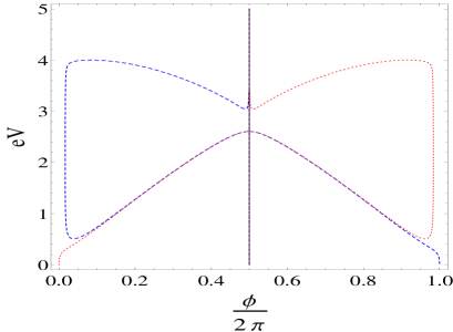
Figure 5: (Color online) Phase diagram for bond currents in the molecular ring. The two curves (red-dotted and blue-dashed) separate regions where both the branches are conducting and black line represents a region where both the branches are non conducting. On the blue (dashed) curve only lower branch is conducting, while on the red (dotted) curve upper branch is conducting. Parameters chosen are $\Gamma=0.1$, $\beta=100$, $\mu=0$, $\mu_{L}=\mu+eV/2$ and $\mu_{R}=\mu-eV/2$.

However we find that, at finite bias ($eV$), $\phi$ can be tuned (without changing polarity) such that only one of the branches is conducting. This is shown in Fig.5, where the white region in $\phi$-$eV$ space indicates that both the branches are conducting, the blue (dashed) curve corresponds to $\phi$ and $eV$ values where only lower branch is conducting ($I_{2\rightarrow 1}=0$) and the red (dotted) curve corresponds to $\phi$ and $eV$ values where only the upper branch is conducting ($I_{4\rightarrow 1}=0$). It should be recalled that at $\phi=\pi$, due to destructive interference, both the branches are non conducting and hence net current in the circuit is also zero (Appendix B), irrespective of the applied bias. This is indicated by a black line in the figure.

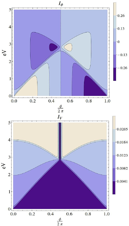
Figure 6: (Color online) Contributions, $I_{\phi}$ (upper panel) and $I_{V}$ (lower panel), to bond currents are plotted as a function of $\phi$ and $eV$ with $\Gamma=0.1$, $\beta=100$, $\mu=0$, $\mu_{L}=\mu+eV/2$ and $\mu_{R}=\mu-eV/2$.

Magnetic field driven ($I_{\phi}$) and applied bias driven ($I_{V}$) contributions to the bond current are plotted in Fig.6 as a function of $\phi$ and $eV$. Notice that $I_{\phi}$ changes sign with respect to both $\phi$ and $eV$, while direction of $I_{V}$ cannot be changed by changing $\phi$. The change in the sign of $I_{\phi}$ with $\phi$ is similar to the case discussed in the thermodynamic equilibrium. However the change in the sign of $I_{\phi}$ with $eV$ happens because, as the bias increases, the populations of states with different contributions changes, resulting in sign change of $I_{\phi}$.

The net current flowing in the circuit for the symmetric ($t=0$) Aharonov-Bohm ring case becomes,

$$I_{L} = \int_{-\infty}^{+\infty}\frac{d\omega}{2\pi}\bigg{[}\frac{4\Gamma^{2}\omega^{2}\cos^{2}(\frac{\phi}{2})}{D[\omega]}\bigg{]}[f_{L}(\omega)-f_{R}(\omega)].$$ (24)

Net current flowing in the circuit has been analyzed in several works to study the effects of the magnetic flux on the net current, for example, Refs. rai ; zeng studied the effect of magnetic field on net transmission function in asymmetric ring system. In Ref. Bai the effect of inhomogeneous magnetic flux on the net current is analyzed. In Ref. Sztenkiel the effect of coulomb interaction on the net current in the presence of magnetic flux is studied. Dissipation due to electron-phonon coupling and its effect on the net transmission has been studied in Ref. Wohlman2 , and the effect of external electromagnetic field has been discussed in Ref. Wohlman1 . In the present work, since we are only interested in bond currents in the molecule, we do not pursue the net current further.

IV Effect of chemical substitution

Here we explore the effect of coupling an extra site (with site energy ’$\epsilon$’ and coupling strength ’t’) to an otherwise symmetric ring system. We analyze the effect of this substitution on the bond currents in the absence of magnetic field. The substitution introduces asymmetry between two paths that an electron can take in going from the left lead to the right lead. This leads to interference effects in the net current as discussed in Refs.Jayannavar2 ; Jayannavar3 . However this asymmetry not only affects the net current but also the bond currents in the molecule and may lead to circulating currents (at finite bias) even in the absence of magnetic flux. The goal in this section is to study these circulating currents. To this end we take the limit $\phi\to 0$ of the general equations (15), (16) and (17), given in Section. II. To further simplify the analysis, we consider the case $\Gamma_{L}=\Gamma_{R}=\Gamma$ and $\epsilon=0$.

The expressions for the bond currents, $I_{2\rightarrow 1}$ and $I_{4\rightarrow 1}$ and the net current, $I_{L}$, assume the form,

$$I_{2\rightarrow 1}=\int_{-\infty}^{+\infty}\frac{d\omega}{2\pi}\bigg{[}\frac{\Gamma^{2}\omega^{2}(2\omega^{2}-t^{2})}{D[\omega]}\bigg{]}\big{[}f_{L}(\omega)-f_{R}(\omega)\big{]},$$

$$I_{4\rightarrow 1}=\int_{-\infty}^{+\infty}\frac{d\omega}{2\pi}\bigg{[}\frac{\Gamma^{2}(\omega^{2}-t^{2})(2\omega^{2}-t^{2})}{D[\omega]}\bigg{]}\big{[}f_{L}(\omega)-f_{R}(\omega)\big{]},$$

$$I_{L}=\int_{-\infty}^{+\infty}\frac{d\omega}{2\pi}\bigg{[}\frac{\Gamma^{2}(2\omega^{2}-t^{2})^{2}}{D[\omega]}\bigg{]}\big{[}f_{L}(\omega)-f_{R}(\omega)\big{]}$$ (27)

where $D[\omega]=\big{[}\omega^{2}+(\frac{\Gamma}{2})^{2}\big{]}\big{[}((\omega^{2}-t^{2})(\omega^{2}-4)-2t^{2})^{2}+(\frac{\Gamma}{2})^{2}\omega^{2}(\omega^{2}-t^{2})^{2}\big{]}$. These currents are plotted as functions of $eV$ and $t$ in Fig.7. Note that the bond current $I_{2\rightarrow 1}$ (corresponding to the branch having the extra substituent) changes sign as bias is scanned, while $I_{4\rightarrow 1}$ remains positive (in the direction of the net current).

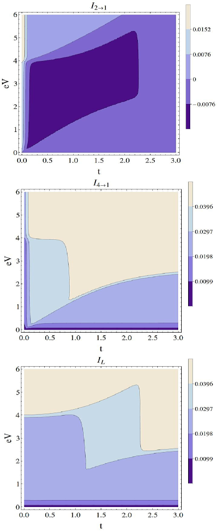
Figure 7: (Color online) Bond currents $I_{2\rightarrow 1}$ and $I_{4\rightarrow 1}$ together with the net current, $I_{L}$, as a function of $t$ and $eV$ with $\epsilon=0$, $\Gamma=0.1$, $\beta=100$, $\mu=0$, $\mu_{L}=\mu+eV/2$ and $\mu_{R}=\mu-eV/2$.

Unlike the case in presence of magnetic flux, in this case the two bond currents (which vanish at zero bias) have well defined energy dependent transmission functions, $T_{12}$ and $T_{14}$. We note that both the transmission functions have common zeros at $\omega=\pm\frac{t}{\sqrt{2}}$. We analyze the nature of transmission functions at these zeros. Since $D[\omega=\pm\frac{t}{\sqrt{2}}]>0$, it is clear that both $T_{12}$ and $T_{14}$ change sign in opposite directions around $\omega=\pm\frac{t}{\sqrt{2}}$. However the total transmission function, $T_{L}(\omega)=\frac{(2\omega^{2}-t^{2})^{2}}{D[\omega]}$ attains its minimum value (zero) at these points (anti-resonances). This behavior of bond transmission functions changing sign around anti-resonances of the total transmission function was noticed by Jayannavar et.al., Jayannavar1 using scattering theory. Apart from the anti-resonance points, $T_{14}$ has extra zeros at $\omega=\pm t$, where it is an increasing (decreasing) function at $+t$ ($-t$), and $T_{12}$ has an extra zero at $\omega=0$ where it has a maximum. For $|\omega|>t$, both $T_{12}(\omega)$ and $T_{14}(\omega)$ are positive functions of $\omega$. Thus at energies $|\omega|>t$, the two bond currents flow in the same (positive) direction, while for $|\omega|<t$, the two currents flow in the opposite direction and a circulating current exists. The energy range $|\omega|<t$ is, therefore, critical for the existence of a circulating current in the molecule. Thus at low temperatures, the circulating current exists only for $|eV|<t$ (here $\mu=0$ is assumed). In Fig.8 we show a plot of $T_{12}(\omega)$, $T_{14}(\omega)$ and $T_{L}(\omega)$.

Zeros of transmission functions $T_{12}(\omega)$, $T_{14}(\omega)$ and $T_{L}(\omega)$ are analyzed using projection operator method in Appendix D. It is shown in Appendix D that the anti- resonance (multi-path zero) of $T_{L}(\omega)$ at $\omega=\pm\frac{t}{\sqrt{2}}$ is due to the destructive interference between two paths ’$1\rightarrow 2\rightarrow 3$’ and ’$1\rightarrow 4\rightarrow 3$’ that an electron can take through the molecule to go from left lead to right lead. $T_{12}(\omega)$ and $T_{14}(\omega)$ are also zero at $\omega=\pm\frac{t}{\sqrt{2}}$, but they do not have simple interpretation in this scheme. Zero (multi-path zero) of $T_{12}(\omega)$ at $\omega=0$ is (for $\epsilon=0$, another zero at $\omega=\epsilon$ called resonance zero coincides with zero at $\omega=0$), is due to the destructive interference between direct (’$1\rightarrow 2$’) and indirect (’$1\rightarrow 4\rightarrow 3\rightarrow 2$’) paths an electron can take to go from site ’1’ to site ’2’. Zeros of $T_{14}(\omega)$ at $\omega=\pm t$ are due to the destructive interference between direct (’$1\rightarrow 4$’) and indirect paths (’$1\rightarrow 2\rightarrow 3\rightarrow 4$’) an electron can take to go from site ’1’ to site ’4’.

Figure 8: Bond transmission functions $T_{12}$ (dashed), $T_{14}$ (dotted) and net transmission function $T_{L}$ (continuous) as a function of $\omega$ with $\Gamma=1$, $\epsilon=0$ and $t=1$.

Circulating current appears due to the negativity of $I_{12}$ which comes from the negativity of $T_{12}$ in the region $|\omega|<\frac{t}{\sqrt{2}}$, outside which $T_{12}$ is positive. For $\Gamma\rightarrow\infty$ (specifically $\Gamma\gg t$), $T_{12}$ in the region $|\omega|<\frac{t}{\sqrt{2}}$ goes to zero as $T_{12}\approx\frac{(2\omega^{2}-t^{2})}{(\omega^{2}-t^{2})^{2}}\frac{16}{\Gamma^{2}}$ and hence negative contribution to $I_{2\rightarrow 1}$ vanishes asymptotically. Therefore for large $\Gamma$, circulating current vanishes. Thus for sufficiently large bias (with $\mu=0$), greater than $\frac{t}{\sqrt{2}}$, and at low temperatures it is be possible to change the sign of $I_{12}$ (from negative to positive) by tuning the coupling strength, $\Gamma$, (for high temperature this can happen even for $|eV|<\frac{t}{\sqrt{2}}$). Hence it is possible to switch between the phases with and without circulating currents in the molecule by tuning $\Gamma$. This is shown in Fig. (9), where the black region represents circulating current in the ring and white region represents a region with no circulating current. It is clear that, for certain values of $eV$, it is possible to switch between phases with and without circulating current by changing $\Gamma$ values. Note that $T_{14}$ is also negative over a small energy window, $\frac{t}{\sqrt{2}}<|\omega|<t$ which is always compensated by the positive contribution from the region $|\omega|<\frac{t}{\sqrt{2}}$, leading to positive $I_{4\rightarrow 1}$.

Figure 9: Circulating current as a function of $\Gamma$ and $eV$ with $\mu_{L}=\mu+\frac{eV}{2}$, $\mu_{R}=\mu-\frac{eV}{2}$, $\mu=0$, $\beta=100$, $t=1$ and $\epsilon=0$. Here it is shown that switching between phases with circulating current (black region) and without circulating current (white region) can be done by tuning $\Gamma$ for certain $eV$.

V Conclusions

We have studied the bond currents in simple ring shaped molecular junction in presence of asymmetry and magnetic field. First case studied is symmetric Aharonov-Bohm ring coupled to metal leads, where we identified two contributions to bond currents, one induced by applied magnetic field ($I_{\phi}$) and the other due to applied bias ($I_{V}$). These two contributions have different origins, the term $I_{\phi}$ is due to the population terms in eigenstate basis and the term $I_{V}$ is due to the coherences induced by leads between different eigenstates. It is possible to tune the applied bias and the applied magnetic field to completely suppress current across one branch and enhance current across the other branch. Lead induced dephasing suppresses the circulating current which, for large lead couplings, dies off quadratically ($\approx\frac{1}{\Gamma^{2}}$). When an asymmetry is introduced by coupling a substituent on one of its branches, it is possible to generate a circulating current at finite bias, even in the absence of applied magnetic field by tuning the coupling strength of the substituent. Furthermore, we find that it is possible to switch between phases with and without circulating currents by tuning the coupling strength of the molecule with leads.

VI Appendix

VI.1 Eigenstate picture of bond currents in Symmetric Aharonov-Bohm ring

The isolated molecule in the presence of magnetic flux is described by the Hamiltonian expressed in terms of Fock space operators,

$$\hat{H}= \begin{pmatrix}c_{1}^{\dagger}&c_{2}^{\dagger}&c_{3}^{\dagger}&c_{4}^{\dagger}\\ \end{pmatrix}H_{system}\begin{pmatrix}c_{1}\\ c_{2}\\ c_{3}\\ c_{4}\\ \end{pmatrix}$$ (28)

with $H_{system}$ given by Eq.(2). The eigenstates of single particle Hamiltonian (given by Eq.(2)) are given by

$$\psi_{1}=\frac{1}{2}\begin{pmatrix}1\\ 1\\ 1\\ 1\end{pmatrix},\psi_{2}=\frac{1}{2}\begin{pmatrix}-i\\ -1\\ i\\ 1\end{pmatrix},\psi_{3}=\frac{1}{2}\begin{pmatrix}i\\ -1\\ -i\\ 1\end{pmatrix}\text{and }\psi_{4}=\frac{1}{2}\begin{pmatrix}-1\\ 1\\ -1\\ 1\end{pmatrix}$$ (29)

with corresponding energies

$$\epsilon_{1}=-2\cos(\frac{\phi}{4}),\epsilon_{2}=2\sin(\frac{\phi}{4}),\epsilon_{3}=-2\sin(\frac{\phi}{4})\text{and }\epsilon_{4}=2\cos(\frac{\phi}{4})$$ (30)

respectively. Hamiltonian in eigenbasis is expressed as

$$\hat{H}=\sum_{i=1}^{4}\epsilon_{i}A_{i}^{\dagger}A_{i}$$ (31)

where creation/annihilation ($A_{i}^{\dagger}\/A_{i}$) operators in eigenbasis can be expressed in terms of creation/annihilation operators in the local basis as,

$$\begin{pmatrix}A_{1}\\ A_{2}\\ A_{3}\\ A_{4}\end{pmatrix}=\mathcal{U}^{\dagger}\begin{pmatrix}c_{1}\\ c_{2}\\ c_{3}\\ c_{4}\end{pmatrix}$$ (32)

where matrix $\mathcal{U}$ has single particle eigenstates given in Eq.(29) as columns. Similarly, from Eq. (4) and (5), $\hat{I}_{2\rightarrow 1}$ and $\hat{I}_{4\rightarrow 1}$ in eigenbasis is given by

$$\hat{I}_{2\rightarrow 1/4\rightarrow 1} = \frac{i}{\hbar}\begin{pmatrix}A^{{\dagger}}_{1}&A^{{\dagger}}_{2}&A^{{\dagger}}_{3}&A^{{\dagger}}_{4}\end{pmatrix}I_{{bond}_{2\rightarrow 1/4\rightarrow 1}}\begin{pmatrix}A_{1}\\ A_{2}\\ A_{3}\\ A_{4}\end{pmatrix}$$ (33)

where

$$I_{{bond}_{2\rightarrow 1}}=\begin{pmatrix}\frac{1}{2}i\sin(\frac{\phi}{4})&(\frac{1}{4}-\frac{i}{4})(\sin(\frac{\phi}{4})+\cos(\frac{\phi}{4}))&(\frac{1}{4}+\frac{i}{4})(\cos(\frac{\phi}{4})-\sin(\frac{\phi}{4}))&-\frac{1}{2}\cos(\frac{\phi}{4})\\ (-\frac{1}{4}-\frac{i}{4})(\sin(\frac{\phi}{4})+\cos(\frac{\phi}{4}))&\frac{1}{2}i\cos(\frac{\phi}{4})&\frac{1}{2}\sin(\frac{\phi}{4})&(\frac{1}{4}-\frac{i}{4})(\cos(\frac{\phi}{4})-\sin(\frac{\phi}{4}))\\ (-\frac{1}{4}+\frac{i}{4})(\cos(\frac{\phi}{4})-\sin(\frac{\phi}{4}))&-\frac{1}{2}\sin(\frac{\phi}{4})&-\frac{1}{2}i\cos(\frac{\phi}{4})&(\frac{1}{4}+\frac{i}{4})(\sin(\frac{\phi}{4})+\cos(\frac{\phi}{4}))\\ \frac{1}{2}\cos(\frac{\phi}{4})&(-\frac{1}{4}-\frac{i}{4})(\cos(\frac{\phi}{4})-\sin(\frac{\phi}{4}))&(-\frac{1}{4}+\frac{i}{4})(\sin(\frac{\phi}{4})+\cos(\frac{\phi}{4}))&-\frac{1}{2}i\sin(\frac{\phi}{4})\end{pmatrix}$$

and

$$I_{{bond}_{4\rightarrow 1}}=\begin{pmatrix}-\frac{1}{2}i\sin(\frac{\phi}{4})&(-\frac{1}{4}-\frac{i}{4})(\cos(\frac{\phi}{4})+\sin(\frac{\phi}{4}))&(-\frac{1}{4}+\frac{i}{4})(\cos(\frac{\phi}{4})-\sin(\frac{\phi}{4}))&-\frac{1}{2}\cos(\frac{\phi}{4})\\ (\frac{1}{4}-\frac{i}{4})(\cos(\frac{\phi}{4})+\sin(\frac{\phi}{4}))&-\frac{1}{2}i\cos(\frac{\phi}{4})&\frac{1}{2}\sin(\frac{\phi}{4})&(-\frac{1}{4}-\frac{i}{4})(\cos(\frac{\phi}{4})-\sin(\frac{\phi}{4}))\\ (\frac{1}{4}+\frac{i}{4})(\cos(\frac{\phi}{4})-\sin(\frac{\phi}{4}))&-\frac{1}{2}\sin(\frac{\phi}{4})&\frac{1}{2}i\cos(\frac{\phi}{4})&(-\frac{1}{4}+\frac{i}{4})(\cos(\frac{\phi}{4})+\sin(\frac{\phi}{4}))\\ \frac{1}{2}\cos(\frac{\phi}{4})&(\frac{1}{4}-\frac{i}{4})(\cos(\frac{\phi}{4})-\sin(\frac{\phi}{4}))&(\frac{1}{4}+\frac{i}{4})(\cos(\frac{\phi}{4})+\sin(\frac{\phi}{4}))&\frac{1}{2}i\sin(\frac{\phi}{4})\end{pmatrix}.$$

Here diagonal elements of $I_{{bond}_{\alpha\rightarrow 1}}$ multiplied by their respective populations give bond currents (between sites ’$\alpha$’ and ’1’ for $\alpha=2,4$) carried by different eigenstates.

It is clear that in isolated molecule described by a thermal ensemble, only populations contribute to bond currents. But if the molecule is connected to leads, coherences can be induced between eigenstates and hence bond currents also change. It is clear, contrary to the recent work Archak , eigenstate Lindblad master equation can give nonzero bond currents (as eigenstates themselves carry finite currents), albeit a wrong result out of equilibrium.

Lesser Green’s function matrix, $G^{<}(\omega)$, can be transformed into eigenbasis as, $\tilde{G}^{<}(\omega)=\mathcal{U}^{{\dagger}}G^{<}(\omega)\mathcal{U}$. From this, bond currents are calculated using, $I_{\alpha\rightarrow 1}=\int^{+\infty}_{-\infty}\frac{d\omega}{2\pi}Tr[I_{{bond}_{\alpha\rightarrow 1}}\tilde{G}^{<}(\omega)]$ for $\alpha=2,4$. By explicit calculation it can be seen (for the case $\Gamma_{L}=\Gamma_{R}=\Gamma$) that, $I_{2\rightarrow 1}=I_{V}+I_{\phi}$ and $I_{4\rightarrow 1}=I_{V}-I_{\phi}$, where only population terms of $\tilde{G}^{<}(\omega)$ contribute to $I_{\phi}$ and coherences contribute to $I_{V}$.

For thermodynamic equilibrium (i.e., $\mu_{L}=\mu_{R}=\mu$ and $\beta_{L}=\beta_{R}=\beta$), eigenstate energies, eigenstate populations ($-i\int_{-\infty}^{+\infty}\frac{d\omega}{2\pi}G_{mm}^{<}(\omega)$) and eigenstate contributions to $I_{\phi}$ are periodic in $\phi$ with period $8\pi$ as shown in Figs. (13), (13) and (13). The net contribution of each eigenstate is also periodic in $\phi$ with period $8\pi$ as shown in Fig. (13), but $I_{\phi}$ is periodic in $\phi$ with period $2\pi$ as can be seen in Fig. (14). This is because eigenstate energies, eigenstate contributions ($I_{{bond}_{{2\rightarrow 1}_{mm}}}$) to $I_{\phi}$ and eigenstate populations get swapped after $2\pi$ increment in $\phi$ as can be seen in Figs. (13), (13) and (13). Furthermore, for $\phi=\pi$, states with opposites contributions to current $I_{\phi}$ become degenerate, hence the circulating current vanishes.

Figure 10: Eigenvalues of isolated ring as a function of $\phi$. Dashed, thick, dotted and thin curves represent eigenstate energies of states 1, 2, 3 and 4.

Figure 11: Contribution of various eigenstates to $I_{\phi}$ as a function of $\phi$. Dashed, thick, dotted and thin curves represent contribution of eigenstates 1, 2, 3 and 4 to $I_{\phi}$.

Figure 12: Populations of various eigenstates of ring connected to reservoir as a function of $\phi$ with $\mu=0$, $eV=0$, $\beta=1$ and $\Gamma=0.1$. Dashed, thick, dotted and thin curves represent populations of eigenstates 1, 2, 3 and 4.

Figure 13: Individual contributions of eigenstates as a function of $\phi$ with $\mu=0$, $eV=0$, $\beta=1$ and $\Gamma=0.1$. Dashed, thick, dotted and thin curves represent individual contributions of eigenstates 1, 2, 3 and 4 to $I_{\phi}$.

Figure 14: $I_{\phi}$ as a function of $\phi$ with $\mu=0$, $eV=0$, $\beta=1$ and $\Gamma=0.1$.

VI.2 Spatial path picture of net current in symmetric Aharonov-Bohm ring

For non interacting electron systems considered here, the net current in the circuit (which can be obtained by using Eq. (14) in Eq. (8)) can be expressed as,

$$I_{L} = \int_{-\infty}^{+\infty}\frac{d\omega}{2\pi}[\Gamma_{L}G^{r}_{13}(\omega)\Gamma_{R}G^{a}_{31}(\omega)][f_{L}(\omega)-f_{R}(\omega)].$$ (36)

Following Ref. Hansen , we use projection operator technique to project out sites ’2’ and ’4’ and obtain,

$$G^{r}_{13}(\omega)=\frac{1}{\omega+i\frac{\Gamma_{L}}{2}-\Sigma_{11}^{Upper}-\Sigma_{11}^{Lower}-\frac{(\Sigma_{13}^{Upper}+\Sigma_{13}^{Lower})(\Sigma_{31}^{Upper}+\Sigma_{31}^{Lower})}{\omega+i\frac{\Gamma_{R}}{2}-\Sigma_{33}^{Upper}-\Sigma_{33}^{Lower}}}\times(\Sigma_{13}^{Upper}+\Sigma_{13}^{Lower})\times\frac{1}{\omega+i\frac{\Gamma_{R}}{2}-\Sigma_{33}^{Upper}-\Sigma_{33}^{Lower}}.$$ (37)

The first term in the product corresponds to renormalized retarded Green’s function for site ’1’ with self energies coming from excursions into upper branch ($\Sigma_{11}^{Upper}$), lower branch ($\Sigma_{11}^{Lower}$) and to and fro excursions to site ’3’ ($\frac{(\Sigma_{13}^{Upper}+\Sigma_{13}^{Lower})(\Sigma_{31}^{Upper}+\Sigma_{31}^{Lower})}{\omega+i\frac{\Gamma_{R}}{2}-\Sigma_{33}^{Upper}-\Sigma_{33}^{Lower}}$). The second term corresponds to the sum of bare amplitudes to go from site ’1’ to site ’3’ through upper ($\Sigma_{13}^{Upper}$) and lower branches ($\Sigma_{13}^{Lower}$). The third term corresponds to the retarded Green’s function for site ’3’ with self energies coming from excursions into upper branch ($\Sigma_{33}^{Upper}$) and lower branch ($\Sigma_{33}^{Lower}$) only. $\Sigma^{Upper/Lower}_{ab}$ are matrix elements of self energies due to upper or lower branches respectively and they are given by $\Sigma^{Upper}=\frac{1}{\omega}\begin{pmatrix}1&&e^{i\frac{\phi}{2}}\\ e^{-i\frac{\phi}{2}}&&1\end{pmatrix}$ and $\Sigma^{Lower}=\frac{1}{\omega}\begin{pmatrix}1&&e^{-i\frac{\phi}{2}}\\ e^{i\frac{\phi}{2}}&&1\end{pmatrix}$. $G^{a}_{31}(\omega)$ can be obtained as $G^{a}_{31}(\omega)=(G^{r}_{13}(\omega))^{*}|_{\phi\rightarrow-\phi}$. For $\phi=\pi$, the two pathways $1\rightarrow 2\rightarrow 3$ and $1\rightarrow 4\rightarrow 3$ destructively interfere (since $(\Sigma_{13}^{Upper}+\Sigma_{13}^{Lower})|_{\phi=\pi}=(\frac{e^{i\frac{\phi}{2}}}{\omega}+\frac{e^{-i\frac{\phi}{2}}}{\omega})|_{\phi=\pi}=0$) leading to zero net current in the circuit. Also for $\phi\neq 2n\pi$ (’n’ is any integer), the net transmission function $T_{L}(\omega)=\Gamma_{L}G^{r}_{13}(\omega)\Gamma_{R}G^{a}_{31}(\omega)$ has a zero (anti-resonance) at $\omega=0$, which is a resonance zero Hansen (since the particle injected from lead into the system at this energy is in resonance with sites ’2’ and ’4’).

VI.3 Analytical expressions for currents for the Symmetric Aharonov-Bohm ring

Finite temperature expressions

$\omega$ integrals in Eqs. (19) and (20) can be performed using contour integration technique to get,

$$I_{V} = \frac{\Gamma^{2}\cos^{2}(\frac{\phi}{2})}{2\pi}\times$$

$$\bigg{[}\frac{ia_{1}}{(a_{1}^{2}-a_{2}^{2})(a_{1}^{2}-a_{3}^{2})(a_{1}^{2}-a_{4}^{2})}\times$$

$$\Big{\{}\Psi[\frac{1}{2}-i\frac{\beta}{2\pi}(\mu_{L}+ia_{1})]-\Psi[\frac{1}{2}+i\frac{\beta}{2\pi}(\mu_{L}-ia_{1})]+\Psi[\frac{1}{2}+i\frac{\beta}{2\pi}(\mu_{R}-ia_{1})]-\Psi[\frac{1}{2}-i\frac{\beta}{2\pi}(\mu_{R}+ia_{1})]\Big{\}}$$

$$+ \frac{ia_{2}}{(a_{2}^{2}-a_{1}^{2})(a_{2}^{2}-a_{3}^{2})(a_{2}^{2}-a_{4}^{2})}\times$$

$$\Big{\{}\Psi[\frac{1}{2}-i\frac{\beta}{2\pi}(\mu_{L}+ia_{2})]-\Psi[\frac{1}{2}+i\frac{\beta}{2\pi}(\mu_{L}-ia_{2})]+\Psi[\frac{1}{2}+i\frac{\beta}{2\pi}(\mu_{R}-ia_{2})]-\Psi[\frac{1}{2}-i\frac{\beta}{2\pi}(\mu_{R}+ia_{2})]\Big{\}}$$

$$+ \frac{ia_{3}}{(a_{3}^{2}-a_{1}^{2})(a_{3}^{2}-a_{2}^{2})(a_{3}^{2}-a_{4}^{2})}\times$$

$$\Big{\{}\Psi[\frac{1}{2}-i\frac{\beta}{2\pi}(\mu_{L}+ia_{3})]-\Psi[\frac{1}{2}+i\frac{\beta}{2\pi}(\mu_{L}-ia_{3})]+\Psi[\frac{1}{2}+i\frac{\beta}{2\pi}(\mu_{R}-ia_{3})]-\Psi[\frac{1}{2}-i\frac{\beta}{2\pi}(\mu_{R}+ia_{3})]\Big{\}}$$

$$+ \frac{ia_{4}}{(a_{4}^{2}-a_{1}^{2})(a_{4}^{2}-a_{2}^{2})(a_{4}^{2}-a_{3}^{2})}\times$$

$$\Big{\{}\Psi[\frac{1}{2}-i\frac{\beta}{2\pi}(\mu_{L}+ia_{4})]-\Psi[\frac{1}{2}+i\frac{\beta}{2\pi}(\mu_{L}-ia_{4})]+\Psi[\frac{1}{2}+i\frac{\beta}{2\pi}(\mu_{R}-ia_{4})]-\Psi[\frac{1}{2}-i\frac{\beta}{2\pi}(\mu_{R}+ia_{4})]\Big{\}}\bigg{]}$$

and

$$I_{\phi} = \frac{\Gamma\sin(\phi)}{2\pi}\times$$

$$\bigg{[}\frac{a_{1}^{2}+2}{(a_{1}^{2}-a_{2}^{2})(a_{1}^{2}-a_{3}^{2})(a_{1}^{2}-a_{4}^{2})}\times$$

$$\Big{\{}\Psi[\frac{1}{2}+i\frac{\beta}{2\pi}(\mu_{L}-ia_{1})]+\Psi[\frac{1}{2}-i\frac{\beta}{2\pi}(\mu_{L}+ia_{1})]+\Psi[\frac{1}{2}+i\frac{\beta}{2\pi}(\mu_{R}-ia_{1})]+\Psi[\frac{1}{2}-i\frac{\beta}{2\pi}(\mu_{R}+ia_{1})]\Big{\}}$$

$$+ \frac{a_{2}^{2}+2}{(a_{2}^{2}-a_{1}^{2})(a_{2}^{2}-a_{3}^{2})(a_{2}^{2}-a_{4}^{2})}\times$$

$$\Big{\{}\Psi[\frac{1}{2}+i\frac{\beta}{2\pi}(\mu_{L}-ia_{2})]+\Psi[\frac{1}{2}-i\frac{\beta}{2\pi}(\mu_{L}+ia_{2})]+\Psi[\frac{1}{2}+i\frac{\beta}{2\pi}(\mu_{R}-ia_{2})]+\Psi[\frac{1}{2}-i\frac{\beta}{2\pi}(\mu_{R}+ia_{2})]\Big{\}}$$

$$+ \frac{a_{3}^{2}+2}{(a_{3}^{2}-a_{1}^{2})(a_{3}^{2}-a_{2}^{2})(a_{3}^{2}-a_{4}^{2})}\times$$

$$\Big{\{}\Psi[\frac{1}{2}+i\frac{\beta}{2\pi}(\mu_{L}-ia_{3})]+\Psi[\frac{1}{2}-i\frac{\beta}{2\pi}(\mu_{L}+ia_{3})]+\Psi[\frac{1}{2}+i\frac{\beta}{2\pi}(\mu_{R}-ia_{3})]+\Psi[\frac{1}{2}-i\frac{\beta}{2\pi}(\mu_{R}+ia_{3})])\Big{\}}$$

$$+ \frac{a_{4}^{2}+2}{(a_{4}^{2}-a_{1}^{2})(a_{4}^{2}-a_{2}^{2})(a_{4}^{2}-a_{3}^{2})}\times$$

$$\Big{\{}\Psi[\frac{1}{2}+i\frac{\beta}{2\pi}(\mu_{L}-ia_{4})]+\Psi[\frac{1}{2}-i\frac{\beta}{2\pi}(\mu_{L}+ia_{4})]+\Psi[\frac{1}{2}+i\frac{\beta}{2\pi}(\mu_{R}-ia_{4})]+\Psi[\frac{1}{2}-i\frac{\beta}{2\pi}(\mu_{R}+ia_{4})]\Big{\}}\bigg{]},$$

where $a_{1}=\frac{\Gamma+\sqrt{\Gamma^{2}-64\sin^{2}(\frac{\phi}{4})}}{4}$, $a_{2}=\frac{\Gamma-\sqrt{\Gamma^{2}-64\sin^{2}(\frac{\phi}{4})}}{4}$, $a_{3}=\frac{\Gamma+\sqrt{\Gamma^{2}-64\cos^{2}(\frac{\phi}{4})}}{4}$, $a_{4}=\frac{\Gamma-\sqrt{\Gamma^{2}-64\cos^{2}(\frac{\phi}{4})}}{4}$ and $\Psi[z]$ is digamma function in variable ’z’ Thomson .

Zero temperature expressions

$\omega$ integrals can be performed after taking zero temperature ($\beta\to\infty$) limits in Eqs. (19) and (20) to get,

$$I_{V} = 2\Gamma^{2}\cos^{2}(\frac{\phi}{2})\times$$

$$\bigg{[}\frac{a_{1}}{(a_{1}^{2}-a_{2}^{2})(a_{1}^{2}-a_{3}^{2})(a_{1}^{2}-a_{4}^{2})}\big{[}\arctan(\frac{\mu_{L}}{a_{1}})-\arctan(\frac{\mu_{R}}{a_{1}})\big{]}+\frac{a_{2}}{(a_{2}^{2}-a_{1}^{2})(a_{2}^{2}-a_{3}^{2})(a_{2}^{2}-a_{4}^{2})}\big{[}\arctan(\frac{\mu_{L}}{a_{2}})-\arctan(\frac{\mu_{R}}{a_{2}})\big{]}$$

$$+ \frac{a_{3}}{(a_{3}^{2}-a_{1}^{2})(a_{3}^{2}-a_{2}^{2})(a_{3}^{2}-a_{4}^{2})}\big{[}\arctan(\frac{\mu_{L}}{a_{3}})-\arctan(\frac{\mu_{R}}{a_{3}})\big{]}+\frac{a_{4}}{(a_{4}^{2}-a_{1}^{2})(a_{4}^{2}-a_{2}^{2})(a_{4}^{2}-a_{3}^{2})}\big{[}\arctan(\frac{\mu_{L}}{a_{4}})-\arctan(\frac{\mu_{R}}{a_{4}})\big{]}\bigg{]}$$

and

$$I_{\phi} = 2\Gamma\sin(\phi)\times$$

$$\bigg{[}\frac{a_{1}^{2}+2}{(a_{1}^{2}-a_{2}^{2})(a_{1}^{2}-a_{3}^{2})(a_{1}^{2}-a_{4}^{2})}\big{[}\ln(\mu_{L}^{2}+a_{1}^{2})+\ln(\mu_{R}^{2}+a_{1}^{2})\big{]}+\frac{a_{2}^{2}+2}{(a_{2}^{2}-a_{1}^{2})(a_{2}^{2}-a_{3}^{2})(a_{2}^{2}-a_{4}^{2})}\big{[}\ln(\mu_{L}^{2}+a_{2}^{2})+\ln(\mu_{R}^{2}+a_{2}^{2})\big{]}$$

$$+ \frac{a_{3}^{2}+2}{(a_{3}^{2}-a_{1}^{2})(a_{3}^{2}-a_{2}^{2})(a_{3}^{2}-a_{4}^{2})}\big{[}\ln(\mu_{L}^{2}+a_{3}^{2})+\ln(\mu_{R}^{2}+a_{3}^{2})\big{]}+\frac{a_{4}^{2}+2}{(a_{4}^{2}-a_{1}^{2})(a_{4}^{2}-a_{2}^{2})(a_{4}^{2}-a_{3}^{2})}\big{[}\ln(\mu_{L}^{2}+a_{4}^{2})+\ln(\mu_{R}^{2}+a_{4}^{2})\big{]}\bigg{]}.$$

VI.4 Interpretation of zeros of Transmission functions for asymmetric ring junction

Using Eq. (14) in Eq. (8), the net current in the circuit can be recast as,

$$I_{L}=$$

$$\int_{-\infty}^{+\infty}\frac{d\omega}{2\pi}[\Gamma_{L}G^{r}_{13}(\omega)\Gamma_{R}G^{a}_{31}(\omega)][f_{L}(\omega)-f_{R}(\omega)].$$ (42)

Similar to Appendix B, we project out sites ’2’, ’4’ and ’5’ to obtain expression for $G^{r}_{13}(\omega)$ as,

$$G^{r}_{13}(\omega)=\frac{1}{\omega+i\frac{\Gamma_{L}}{2}-\Sigma_{11}^{Upper}-\Sigma_{11}^{Lower}-\frac{(\Sigma_{13}^{Upper}+\Sigma_{13}^{Lower})(\Sigma_{31}^{Upper}+\Sigma_{31}^{Lower})}{\omega+i\frac{\Gamma_{R}}{2}-\Sigma_{33}^{Upper}-\Sigma_{33}^{Lower}}}\times(\Sigma_{13}^{Upper}+\Sigma_{13}^{Lower})\times\frac{1}{\omega+i\frac{\Gamma_{R}}{2}-\Sigma_{33}^{Upper}-\Sigma_{33}^{Lower}},$$ (43)

The interpretation of three terms in $G^{a}_{13}(\omega)$ is same as discussed in Appendix B. $\Sigma^{Upper/Lower}_{ab}$ are matrix elements of self energies due to upper (lower) branch, they are given by $\Sigma^{Upper}=\frac{(\omega-\epsilon)}{\omega(\omega-\epsilon)-t^{2}}\begin{pmatrix}1&&1\\ 1&&1\end{pmatrix}$ and $\Sigma^{Lower}=\frac{1}{\omega}\begin{pmatrix}1&&1\\ 1&&1\end{pmatrix}$. $G^{a}_{31}(\omega)$ can be obtained as $G^{a}_{31}(\omega)=(G^{r}_{13}(\omega))^{*}$. For $\omega=\frac{\epsilon\pm\sqrt{\epsilon^{2}+2t^{2}}}{2}$, the two pathways $1\rightarrow 2\rightarrow 3$ and $1\rightarrow 4\rightarrow 3$ destructively interfere (since $(\Sigma_{13}^{Upper}+\Sigma_{13}^{Lower})|_{\omega=\frac{\epsilon\pm\sqrt{\epsilon^{2}+2t^{2}}}{2}}=0$) leading to zeros (anti-resonances) in the net transmission coefficient (termed as multi-path zeros due to their origin from destructive interference between the two paths) Hansen . However in the presence of applied magnetic field, these anti resonances in $T_{L}(\omega)$ disappear (Eq. (17)).

Using Eq. (14) in Eqs. (6) and (7) (additionally using $Im[G^{r}_{13}(\omega)G^{a}_{32}(\omega)]=-Im[G^{r}_{11}(\omega)G^{a}_{12}(\omega)]$ and $Im[G^{r}_{13}(\omega)G^{a}_{34}(\omega)]=-Im[G^{r}_{11}(\omega)G^{a}_{14}(\omega)]$ for $\phi=0$ case), expressions for the two bond currents $I_{2\rightarrow 1}$ and $I_{4\rightarrow 1}$, given by Eqs. (6) and (7) with $\phi=0$ and $\Gamma_{L}=\Gamma_{R}=\Gamma$ can be cast as,

$$I_{2\rightarrow 1}=$$

$$-2\int_{-\infty}^{+\infty}\frac{d\omega}{2\pi}\Gamma Im[G^{r}_{11}(\omega)G^{a}_{12}(\omega)][f_{L}(\omega)-f_{R}(\omega)],$$ (44)

$$I_{4\rightarrow 1}=$$

$$-2\int_{-\infty}^{+\infty}\frac{d\omega}{2\pi}\Gamma Im[G^{r}_{11}(\omega)G^{a}_{14}(\omega)][f_{L}(\omega)-f_{R}(\omega)].$$ (45)

To analyze zeros of transmission function $T_{12}(\omega)=-2\Gamma Im[G^{r}_{11}(\omega)G^{a}_{12}(\omega)]$, for the current between sites ’1’ and ’2’, we follow the same procedure as above and project out sites ’3’, ’4’ and ’5’ to get,

$$G^{r}_{11}(\omega)=\frac{1}{\omega+i\frac{\Gamma}{2}-\Sigma^{Indirect}_{11}-\frac{(\Sigma^{Direct}_{12}+\Sigma^{Indirect}_{12})(\Sigma^{Direct}_{21}+\Sigma^{Indirect}_{21})}{\omega-\Sigma^{Indirect}_{22}-\Sigma^{Substituent}_{22}}}$$ (46)

and

$$G^{a}_{12}(\omega)=\frac{1}{\omega-i\frac{\Gamma}{2}-(\Sigma^{Indirect}_{11})^{*}-\frac{((\Sigma^{Direct}_{12})^{*}+(\Sigma^{Indirect}_{12})^{*})((\Sigma^{Direct}_{21})^{*}+(\Sigma^{Indirect}_{21})^{*})}{\omega-(\Sigma^{Indirect}_{22})^{*}-(\Sigma^{Substituent}_{22})^{*}}}$$

$$\times((\Sigma^{Direct}_{12})^{*}+(\Sigma^{Indirect}_{12})^{*})\frac{1}{\omega-(\Sigma^{Indirect}_{22})^{*}-(\Sigma^{Substituent}_{22})^{*}}.$$ (47)

$\Sigma^{Direct/Indirect}_{ab}$ are matrix elements of self energies due to direct path ’$1\rightarrow 2$’ (indirect path ’$1\rightarrow 4\rightarrow 3\rightarrow 2$’) given by $\Sigma^{Direct}=\begin{pmatrix}0&&-1\\ -1&&0\end{pmatrix}$ and $\Sigma^{Direct}=\begin{pmatrix}\frac{1}{\omega-\frac{1}{\omega+i\frac{\Gamma}{2}}}&&-\frac{1}{\omega}\frac{1}{\omega+i\frac{\Gamma}{2}-\frac{1}{\omega}}\\ -\frac{1}{\omega+i\frac{\Gamma}{2}-\frac{1}{\omega}}\frac{1}{\omega}&&\frac{1}{\omega+i\frac{\Gamma}{2}-\frac{1}{\omega}}\end{pmatrix}$, self energy due to extra substituent is $\Sigma^{Substituent}=\begin{pmatrix}0&&0\\ 0&&\frac{t^{2}}{\omega-\epsilon}\end{pmatrix}$. At $\omega=\epsilon$, $G^{a}_{12}(\omega)$ becomes zero (due to the bare advanced Green’s function term becoming zero due to divergence of $\Sigma_{22}^{Substituent}$), leading to zero of the transmission function (termed as resonance zero). Another zero (multi-path zero) of the transmission function can be identified at $\omega=0$, where $(\Sigma^{Direct}_{12})^{*}+(\Sigma^{Inirect}_{12})^{*}=-\frac{\omega}{\omega(\omega-i\frac{\Gamma}{2})-1}$ becomes zero, which can be interpreted as a result of destructive interference between direct and indirect paths. Another set of zeros (which are multi-path zeros of net transmission function $T_{L}(\omega)$ at $\omega=\frac{\epsilon\pm\sqrt{\epsilon^{2}+2t^{2}}}{2}$ discussed above) does not have a simple interpretation in this procedure.

For analyzing zeros of transmission function $T_{14}(\omega)=-2\Gamma Im[G^{r}_{11}(\omega)G^{a}_{14}(\omega)]$, for the current between sites ’1’ and ’4’, we project out sites ’2’, ’3’ and ’5’ to get,

$$G^{r}_{11}(\omega)=\frac{1}{\omega+i\frac{\Gamma}{2}-\Sigma^{Indirect}_{11}-\frac{(\Sigma^{Direct}_{14}+\Sigma^{Indirect}_{14})(\Sigma^{Direct}_{41}+\Sigma^{Indirect}_{41})}{\omega-\Sigma^{Indirect}_{44}}}$$ (48)

and

$$G^{a}_{14}(\omega)=\frac{1}{\omega-i\frac{\Gamma}{2}-(\Sigma^{Indirect}_{11})^{*}-\frac{((\Sigma^{Direct}_{14})^{*}+(\Sigma^{Indirect}_{14})^{*})((\Sigma^{Direct}_{41})^{*}+(\Sigma^{Indirect}_{41})^{*})}{\omega-(\Sigma^{Indirect}_{44})^{*}}}$$

$$\times((\Sigma^{Direct}_{14})^{*}+(\Sigma^{Indirect}_{14})^{*})\frac{1}{\omega-(\Sigma^{Indirect}_{44})^{*}}.$$ (49)

$\Sigma^{Direct/Indirect}_{ab}$ are matrix elements of self energies due to direct path ’$1\rightarrow 4$’ (indirect path ’$1\rightarrow 2\rightarrow 3\rightarrow 4$’) given by $\Sigma^{Direct}=\begin{pmatrix}0&&-1\\ -1&&0\end{pmatrix}$ and $\Sigma^{Direct}=\frac{1}{[(\omega+i\frac{\Gamma}{2})\{\omega(\omega-\epsilon)-t^{2}\}-(\omega-\epsilon)]}\begin{pmatrix}(\omega-\epsilon)(\omega+i\frac{\Gamma}{2})&&-(\omega-\epsilon)\\ -(\omega-\epsilon)&&\omega(\omega-\epsilon)-t^{2}\end{pmatrix}$. At $\omega=\frac{\epsilon\pm\sqrt{\epsilon^{2}+4t^{2}}}{2}$, $(\Sigma^{Direct}_{14})^{*}+(\Sigma^{Inirect}_{14})^{*}=\frac{(\omega+i\frac{\Gamma}{2})\{\omega(\omega-\epsilon)-t^{2}\}}{[(\omega+i\frac{\Gamma}{2})\{\omega(\omega-\epsilon)-t^{2}\}-(\omega-\epsilon)]}$ becomes zero, hence $\omega=\frac{\epsilon\pm\sqrt{\epsilon^{2}+4t^{2}}}{2}$ are zeros of $T_{14}(\omega)$ (these zeros are a result of destructive interference between direct and indirect paths and hence can be termed as multi-path zeros). Similar to $T_{12}(\omega)$ case, another set of zeros (at $\omega=\frac{\epsilon\pm\sqrt{\epsilon^{2}+2t^{2}}}{2}$) does not have a simple interpretation in this procedure.

References

• (1) Yoseph Imry. Introduction to mesoscopic physics. Number 2. Oxford University Press on Demand, 2002.
• (2) Linus Pauling. The diamagnetic anisotropy of aromatic molecules. The Journal of Chemical Physics, 4(10):673–677, 1936.
• (3) N Byers and CN Yang. Theoretical considerations concerning quantized magnetic flux in superconducting cylinders. Physical review letters, 7(2):46, 1961.
• (4) M Büttiker, Yoseph Imry, and Rolf Landauer. Josephson behavior in small normal one-dimensional rings. Physics letters a, 96(7):365–367, 1983.
• (5) Gemma C Solomon, Carmen Herrmann, Thorsten Hansen, Vladimiro Mujica, and Mark A Ratner. Exploring local currents in molecular junctions. Nature chemistry, 2(3):223–228, 2010.
• (6) Dhurba Rai, Oded Hod, and Abraham Nitzan. Magnetic field control of the current through molecular ring junctions. The Journal of Physical Chemistry Letters, 2(17):2118–2124, 2011.
• (7) Oded Hod, Eran Rabani, and Roi Baer. Magnetoresistance of nanoscale molecular devices. Accounts of chemical research, 39(2):109–117, 2006.
• (8) Oded Hod, Roi Baer, and Eran Rabani. Magnetoresistance of nanoscale molecular devices based on aharonov–bohm interferometry. Journal of Physics: Condensed Matter, 20(38):383201, 2008.
• (9) Dhurba Rai, Oded Hod, and Abraham Nitzan. Circular currents in molecular wires†. The Journal of Physical Chemistry C, 114(48):20583–20594, 2010.
• (10) Dhurba Rai, Oded Hod, and Abraham Nitzan. Magnetic fields effects on the electronic conduction properties of molecular ring structures. Physical Review B, 85(15):155440, 2012.
• (11) AM Jayannavar, P Singha Deo, and TP Pareek. Current magnification and circulating currents in mesoscopic rings. Physica B: Condensed Matter, 212(3):261–266, 1995.
• (12) Maria A Davidovich, VM Apel, EV Anda, and G Chiappe. Currents along ring arms with quantum dots: Kondo and aharonov–bohm effects. Journal of Magnetism and Magnetic Materials, 320(14):e246–e248, 2008.
• (13) R Peierls. On the theory of diamagnetism of conduction electrons. Z. Phys, 80:763–791, 1933.
• (14) Hartmut Haug, Antti-Pekka Jauho, and M Cardona. Quantum kinetics in transport and optics of semiconductors, volume 14. Springer, 2008.
• (15) Jørgen Rammer. Quantum field theory of non-equilibrium states. Cambridge University Press, 2007.
• (16) ZY Zeng, F Claro, and Alejandro Pérez. Fano resonances and aharonov-bohm effects in transport through a square quantum dot molecule. Physical Review B, 65(8):085308, 2002.
• (17) Archak Purkayastha, Manas Kulkarni, and Abhishek Dhar. Exact redfield description for open non-interacting quantum systems and failure of the lindblad approach. arXiv preprint arXiv:1511.03778, 2015.
• (18) Sybren Ruurds De Groot and Peter Mazur. Non-equilibrium thermodynamics. Courier Corporation, 2013.
• (19) M Büttiker. Role of quantum coherence in series resistors. Physical Review B, 33(5):3020, 1986.
• (20) M Büttiker. Small normal-metal loop coupled to an electron reservoir. Physical Review B, 32(3):1846, 1985.
• (21) L Melville Milne-Thomson, M Abramowitz, and IA Stegun. Handbook of mathematical functions. Handbook of Mathematical Functions, 1972.
• (22) Zhi-Ming Bai, Min-Fong Yang, and Yung-Chung Chen. Effect of inhomogeneous magnetic flux on double-dot aharonov–bohm interferometer. Journal of Physics: Condensed Matter, 16(12):2053, 2004.
• (23) D Sztenkiel and R Świrkowicz. Interference effects in a double quantum dot system with inter-dot coulomb correlations. Journal of Physics: Condensed Matter, 19(17):176202, 2007.
• (24) O Entin-Wohlman, Y Imry, and A Aharony. Persistent currents in interacting aharonov-bohm interferometers and their enhancement by acoustic radiation. Physical review letters, 91(4):046802, 2003.
• (25) O Entin-Wohlman, Y Imry, and A Aharony. Effects of external radiation on biased aharonov-bohm rings. Physical Review B, 70(7):075301, 2004.
• (26) TP Pareek, P Singha Deo, and AM Jayannavar. Effect of impurities on the current magnification in mesoscopic open rings. Physical Review B, 52(20):14657, 1995.
• (27) AM Jayannavar and P Singha Deo. Persistent currents in the presence of a transport current. Physical Review B, 51(15):10175, 1995.
• (28) Thorsten Hansen, Gemma C Solomon, David Q Andrews, and Mark A Ratner. Interfering pathways in benzene: An analytical treatment. The Journal of chemical physics, 131(19):194704, 2009.