Interpretable sparse SIR for functional data

Abstract

We propose a semiparametric framework based on Sliced Inverse Regression (SIR) to address the issue of variable selection in functional regression. SIR is an effective method for dimension reduction which computes a linear projection of the predictors in a low-dimensional space, without loss of information on the regression. In order to deal with the high dimensionality of the predictors, we consider penalized versions of SIR: ridge and sparse. We extend the approaches of variable selection developed for multidimensional SIR to select intervals that form a partition of the definition domain of the functional predictors. Selecting entire intervals rather than separated evaluation points improves the interpretability of the estimated coefficients in the functional framework. A fully automated iterative procedure is proposed to find the critical (interpretable) intervals. The approach is proved efficient on simulated and real data. The method is implemented in the R package SISIR available on CRAN at https://cran.r-project.org/package=SISIR. Keywords : functional regression; SIR; Lasso; ridge regression; interval selection.

1 Introduction

This article focuses on the functional regression problem, in which a real random variable $Y$ is predicted from a functional predictor $X(t)$ that takes values in a functional space (e.g., $L^{2}([0,1])$, the space of squared integrable functions over $[0,1]$), based on a set of observed pairs $(X,Y)$, $(\mathbf{x}_{i},y_{i})_{i=1,\ldots,n}$. The main challenge with functional regression lies in its high dimension: the underlying dimension of a functional space is infinite, and even if the digitized version of the curves is considered, the number of evaluation points is typically much larger than the number of observations.

Recently, an increasing number of works have focused on variable selection in this functional regression framework, in particular in the linear setting. The problem is to select parts of the definition domain of $X$ that are relevant to predict $Y$. Considering digitized versions of the functional predictor $X$, approaches based on Lasso have been proposed to select a few isolated points of $X$ (Ferraty et al, 2010; Aneiros and Vieu, 2014; McKeague and Sen, 2010; Kneip et al, 2016). Alternatively, other authors proposed to perform variable selection on predefined functional bases. For instance, Matsui and Konishi (2011) used $L^{1}$ regularization on Gaussian basis functions and Zhao et al (2012); Chen et al (2015) on wavelets.

However, in many practical situations, the relevant information may not correspond to isolated evaluation points of $X$ neither to some of the components of its expansion on a functional basis, but to its value on some continuous intervals, $X(\left[t_{a},t_{b}\right])$. In that case, variable selection amounts to identify those intervals. As advocated by James et al (2009), a desirable feature of variable selection provided by such an approach is to enhance the interpretability of the relation between $X$ and $Y$. Indeed, it reduces the definition domain of the predictors to a few influential intervals, or it focuses on some particular aspects of the curves in order to obtain expected values for $Y$. Tackling this issue can be seen as selecting groups of contiguous variables (i.e., intervals) instead of selecting isolated variables. Fraiman et al (2016), in the linear setting, and Fauvel et al (2015); Ferraty and Hall (2015), in a nonparametric framework, propose several alternatives to do so. However, no specific contiguity constraint is put on groups of variables.

In the present work, we propose a semi-parametric model that selects intervals in the definition domain of $X$ with an automatic approach. The method is based on Sliced Inverse Regression (SIR, Li, 1991): the main idea of SIR is to define a low dimensional data-driven subspace on which the functional predictors can be projected. This subspace, called Effective Dimension Reduction (EDR) space is defined so as to optimize the prediction ability of the projection. As a particular case, the method includes the linear regression. Our choice for SIR is motivated by the fact that the method is based on a semi-parametric model that is more flexible than linear models. The method has been extended to the functional framework in previous works (Ferré and Yao, 2003; Ferré and Villa, 2006) and sparse (i.e., $\ell_{1}$ penalized) versions of the approach have also already been proposed in Li and Nachtsheim (2008) and Li and Yin (2008) for the multivariate framework. Building on these previous proposals, we show that a tailored group-Lasso-like penalty allows us to select groups of variables corresponding to intervals in the definition domain of the functional predictors.

Our second contribution is a fast and automatic procedure for building intervals in the definition domain of the predictors without using any prior knowledge. As far as we know, the only works that propose a method to both define and select relevant intervals in the domain of the predictors are the work of Park et al (2016) and Grollemund et al (2018), both in the linear framework. Our approach is based on an iterative procedure that uses the full regularization path of the Lasso.

The paper is organized as follows: Section 2 presents the SIR approach in a multidimensional framework and its adaptations to the high-dimensional and functional frameworks, which are based on regularization and/or sparsity constraints. Section 3 describes our proposal when the domain of the predictors are partitioned using a fixed set of intervals. Then, Section 4 describes an automatic procedure to find these intervals and Section 5 provides practical methods to tune the different parameters in a high dimensional framework. Finally, Section 6 evaluates our approach on simulated and real-world datasets.

2 A review on SIR and regularized versions

In this section, we review the standard SIR for multivariate data and its extensions to the high-dimensional setting. Here, $(X,Y)$ denotes a random pair of variables such that $X$ takes values in $\mathbb{R}^{p}$ and $Y$ is real. We assume given $n$ i.i.d. realizations of $(X,Y)$, $(\mathbf{x}_{i},y_{i})_{i=1,\ldots,n}$.

2.1 The standard multidimensional case

When $p$ is large, classical modeling approaches suffer from the curse of dimensionality. This problem might occur even if $p$ is smaller than $n$. A standard way to overcome this issue is to rely on dimension reduction techniques. This kind of approaches is based on the assumption that there exists an Effective Dimension Reduction (EDR) space $\mathcal{S}_{Y|X}$ which is the smallest subspace such that the projection of $X$ on $\mathcal{S}_{Y|X}$ retains all the information on $Y$ contained in the predictor $X$. More precisely, $\mathcal{S}_{Y|X}$ is assumed of the form $\mbox{Span}\{\mathbf{a}_{1},\ldots,\mathbf{a}_{d}\}$, with $d\ll p$, such that

$$Y=F(\mathbf{a}_{1}^{\top}X,\ldots,\mathbf{a}_{d}^{\top}X,\epsilon),$$ (1)

in which $F:\mathbb{R}^{p+1}\rightarrow\mathbb{R}$ is an unknown function and $\epsilon$ is an error term independent of $X$. To estimate this subspace, SIR is one of the most classical approaches when $p<n$: under an appropriate and general enough condition, Li (1991) shows that $\mathbf{a}_{1},\ldots,\mathbf{a}_{d}$ can be estimated as the first $d$ $\Sigma$-orthonormal eigenvectors of the generalized eigenvalue problem: $\Gamma\mathbf{a}=\lambda\Sigma\mathbf{a}$, in which $\Sigma$ is the covariance matrix of $X$ and $\Gamma$ is the covariance matrix of $\mathbb{E}(X|Y)$.

In practice, $\Sigma$ is replaced by the empirical covariance, $\widehat{\Sigma}=\frac{1}{n}\sum_{i=1}^{n}\left(\mathbf{x}_{i}-\overline{X}\right)\left(\mathbf{x}_{i}-\overline{X}\right)^{\top}$, and $\Gamma$ is estimated by “slicing” the observations $(y_{i})_{i}$ as follows. The range of $Y$ is partitioned into $H$ consecutive and non-overlapping slices, denoted hereafter $\mathcal{S}_{1}$, …, $\mathcal{S}_{H}$. An estimate of $\mathbb{E}(X|Y)$ is thus simply obtained by $\left(\overline{X}_{1},\ldots,\overline{X}_{H}\right)$ in which $\overline{X}_{h}$ is the average of the observations $\mathbf{x}_{i}$ such that $y_{i}$ is in $\mathcal{S}_{h}$ and $\overline{X}_{h}$ is associated with the empirical frequency $\hat{p}_{h}=\frac{n_{h}}{n}$ with $n_{h}$ the number of observations in $\mathcal{S}_{h}$. $\widehat{\Gamma}$ is thus defined as $\sum_{h=1}^{H}\hat{p}_{h}\overline{X}_{h}\overline{X}_{h}^{\top}$.

SIR has different equivalent formulations that can be useful to introduce regularization and sparsity. Cook (2004) shows that the SIR estimate can be obtained by minimizing over $A\in\mathbb{R}^{p\times d}$ and $C=\left(C_{1},\,...,\,C_{H}\right)$, with $C_{h}\in\mathbb{R}^{d}$ (for $h=1,\ldots,H$),

$$\mathcal{E}_{1}(A,C)=\sum_{h=1}^{H}\hat{p}_{h}\|(\overline{X}_{h}-\overline{X})-\widehat{\Sigma}AC_{h}\|^{2}_{\widehat{\Sigma}^{-1}},$$ (2)

in which $\|.\|_{\widehat{\Sigma}^{-1}}^{2}$ is the norm $\forall\,u\in\mathbb{R}^{p}$, $\|u\|_{\widehat{\Sigma}^{-1}}^{2}=u^{\top}\widehat{\Sigma}^{-1}u$ and the searched vectors $\mathbf{a}_{j}$ are the columns of $A$.

An alternative formulation is described in Chen and Li (1998), where SIR is written as the following optimization problem:

$$\max_{\mathbf{a}_{j},\phi}\mbox{Cor}(\phi(Y),\mathbf{a}_{j}^{\top}X),$$ (3)

where $\phi$ is any function $\mathbb{R}\rightarrow\mathbb{R}$ and $(\mathbf{a}_{j})_{j}$ are $\Sigma$-orthonormal. So, SIR can be interpreted as a canonical correlation problem. The authors also prove that the solution of $\phi$ optimizing Equation (3) for a given $\mathbf{a}_{j}$ is $\phi(y)=\mathbf{a}_{j}^{\top}\mathbb{E}(X|Y=y)$, and that $\mathbf{a}_{j}$ is also obtained as the solution of the mean square error optimization $\min_{\mathbf{a}_{j}}\mathbb{E}\left(\phi(Y)-\mathbf{a}_{j}^{\top}X\right)^{2}$.

However, as explained in Li and Yin (2008) and Coudret et al (2014) among others, in a high dimensional setting ($n<p$), $\widehat{\Sigma}$ is singular and the SIR problem is thus ill-posed. The same problem occurs in the functional setting (Dauxois et al, 2001). Solutions to overcome this difficulty include variable selection (Coudret et al, 2014), ridge regularization or sparsity constraints.

2.2 Regularization in the high-dimensional setting

In the high-dimensional setting, directly applying a ridge penalty, $\mu_{2}\sum_{h=1}^{H}\hat{p}_{h}\|AC_{h}\|_{\mathbb{I}_{p}}^{2}$ (for a given $\mu_{2}>0$), to $\mathcal{E}_{1}$ would require the computation of $\widehat{\Sigma}^{-1}$ (see Equation (2)) that does not exist when $n<p$. However, Bernard-Michel et al (2008) show that this problem can be rewritten as the minimization of

$$\sum_{h=1}^{H}\hat{p}_{h}C_{h}^{\top}A^{\top}(\widehat{\Sigma}+\mu_{2}\mathbb{I}_{p})AC_{h}-$$

$$\qquad\qquad\qquad 2\sum_{h=1}^{H}\hat{p}_{h}\left(\overline{X}_{h}-\overline{X}\right)AC_{h},$$ (4)

which is well defined even for the high-dimensional setting. Minimizing this quantity with respect to $A$ leads to define the columns of $A$ (and hence the searched vectors $\mathbf{a}_{j}$) as the first $d$ eigenvectors of $\left(\widehat{\Sigma}+\mu_{2}\mathbb{I}_{p}\right)^{-1}\widehat{\Gamma}$.

2.3 Sparse SIR

Sparse estimates of $\mathbf{a}_{j}$ usually increase the interpretability of the model (here, of the EDR space) by focusing on the most important predictors only. Also, Lin et al (2018) prove the relevance of sparsity for SIR in high dimensional setting by proposing a consistent screening pre-processing of the variables before the SIR estimation. A different and very commmon approach is to handle sparsity directly by a sparse penalty (in the line of the well-known Lasso). However, contrary to ridge regression, adding directly a sparse penalty to Equation (2) does not allow a reformulation valid for the case $n<p$. To the best of our knowledge, only two alternatives have already been published to use such methods, one based on the regression formulation (2) and the other on the correlation formulation (3) of SIR.

Li and Yin (2008) derive a sparse ridge estimator from the work of Ni et al (2005). Given $(\hat{A},\hat{C})$, solution of the ridge SIR, a shrinkage index vector $\boldsymbol{\alpha}=(\alpha_{1},\ldots,\alpha_{p})^{\top}\in\mathbb{R}^{p}$ is obtained by minimizing a least square error with $\ell_{1}$ penalty:

$$\mathcal{E}_{s,1}(\boldsymbol{\alpha}) = \sum_{h=1}^{H}\hat{p}_{h}\left\|\left(\overline{X}_{h}-\overline{X}\right)-\widehat{\Sigma}\mbox{Diag}(\boldsymbol{\alpha})\hat{A}\hat{C}_{h}\right\|_{\mathbb{I}_{p}}^{2}+$$ (5)

$$\qquad\mu_{1}\|\boldsymbol{\alpha}\|_{\ell_{1}},$$

for a given $\mu_{1}\in\mathbb{R}^{+*}$ where $\|\boldsymbol{\alpha}\|_{\ell_{1}}=\sum_{j=1}^{p}|\alpha_{j}|$. Once the coefficients $\boldsymbol{\alpha}$ have been estimated, the EDR space is the space spanned by the columns of $\mbox{Diag}(\hat{\boldsymbol{\alpha}})\hat{A}$, where $\hat{\boldsymbol{\alpha}}$ is the solution of the minimization of $\mathcal{E}_{s,1}(\boldsymbol{\alpha})$.

An alternative is described in Li and Nachtsheim (2008) using the correlation formulation of the SIR. After the standard SIR estimates $\hat{\mathbf{a}}_{1},\ldots,\hat{\mathbf{a}}_{d}$ have been computed, they solve $d$ independent minimization problems with sparsity constraints introduced as an $\ell_{1}$ penalty: $\forall\,j=1,\ldots,d$,

$$\mathcal{E}_{s,2}(\mathbf{a}^{s}_{j})=\sum_{i=1}^{n}\left[\mathcal{P}_{\hat{\mathbf{a}}_{j}}(X|y_{i})-(\mathbf{a}_{j}^{s})^{\top}\mathbf{x}_{i}\right]^{2}+\mu_{1,j}\|\mathbf{a}_{j}^{s}\|_{\ell_{1}},$$ (6)

in which $\mathcal{P}_{\hat{\mathbf{a}}_{j}}(X|y_{i})=\widehat{\mathbb{E}}(X|Y=y_{i})^{\top}\hat{\mathbf{a}}^{j}$, with $\widehat{\mathbb{E}}(X|Y=y_{i})=\overline{X}_{h}$ for $h$ such that $y_{i}\in\mathcal{S}_{h}$ in the case of a sliced estimate of $\widehat{\mathbb{E}}(X|Y)$ and $\mu_{1,j}>0$ is a parameter controlling the sparsity of the solution.

Note that both proposals have problems in the high-dimensional setting:

• In their proposal, Li and Yin (2008) avoid the issue of the singularity of $\widehat{\Sigma}$ by working in the original scale of the predictors for both the ridge and the sparse approach (hence the use of the $\|.\|_{\mathbb{I}_{p}}$-norm in Equation (5) instead of the standard $\|.\|_{\widehat{\Sigma}^{-1}}$-norm of Equation (2)). However, for the ridge problem, this choice has been proved to produce a degenerate problem by Bernard-Michel et al (2008).

• Li and Nachtsheim (2008) base their sparse version of the SIR on the standard estimates of the SIR problem that cannot be computed in the high-dimensional setting.

Moreover, the other differences between these two approaches can be summarized in two points:

• using the approach of Li and Yin (2008) based on shrinkage coefficients, the indices $\alpha_{j}$ where $\alpha_{j}>0$ are the same on all the $d$ components of the EDR. This makes sense because the vectors $\mathbf{a}_{j}$ themselves are not relevant: only the space spanned by them is and so there is no interest to select different variables $j$ for the $d$ estimated directions. Moreover, this allows to formulate the optimization in a single problem. However, this problem relies on a least square minimization with dependent variables in a high dimensional space $\mathbb{R}^{p}$;

• on the contrary, the approach of Chen and Li (1998) relies on a least square problem based on projections and is thus obtained from $d$ independent optimization problems. The dimension of the dependent variable is reduced (1 instead of $p$) but the different vectors which span the EDR space are estimated independently and not simultaneously.

In our proposal, we combine both advantages of Li and Yin (2008) and Li and Nachtsheim (2008) using a single optimization problem based on the correlation formulation of SIR. In this problem, the dimension of the dependent variable is reduced ($d$ instead of $p$) when compared to the approach of Li and Yin (2008) and it is thus computationally more efficient. Identical sparsity constraints are imposed on all $d$ dimensions using a shrinkage approach, but instead of selecting the nonzero variables independently, we adapt the sparsity constraint to the functional setting to avoid selecting isolated measurement points. The next section describes this approach.

3 Sparse and Interpretable SIR (SISIR)

In this section, a functional regression framework is assumed. $X$ is thus a functional random variable, taking value in a (infinite dimensional) Hilbert space. $(x_{i},y_{i})_{i=1,\ldots,n}$ are $n$ i.i.d. realizations of $(X,Y)$. However, $x_{i}$ are not perfectly known but observed on a given (deterministic) grid $\tau=\{t_{1},\ldots,t_{p}\}$. We denote by $\mathbf{x}_{i}=(x_{i}(t_{j}))_{j=1,\ldots,p}\in\mathbb{R}^{p}$ the $i$-th observation, by $\mathbf{x}^{j}=(x_{i}(t_{j}))_{i=1,\ldots,n}$ the observations at $t_{j}$ and by $\mathbf{X}$ the $n\times p$ matrix $(\mathbf{x}_{1},\ldots,\mathbf{x}_{n})^{\top}$. Unless said otherwise, the notations are derived from the ones introduced in the multidimensional setting (Section 2) by using the $\mathbf{x}_{i}$ as realizations of $X$.

Some very common methods in functional data analysis, such as splines (Hastie et al, 2001), use the supposed smoothness of $X$ to project them in a reduced dimension space. Contrary to these methods, we do not use or need that the observed functional predictor is smooth. We take advantage of the functional aspects of the data in a different way, using the natural ordering of the definition domain of $X$ to impose sparsity on the EDR space. To do so, we assume that this definition domain is partitioned into $D$ contiguous and non-overlapping intervals, $\tau_{1},\ldots,\tau_{D}$. In the present section, these intervals are supposed to be given a priori and we will describe later (in Section 4) a fully automated procedure to obtain them from the data.

The following two subsections are devoted to the description of the two steps (ridge and sparse) of the method, adapted from Bernard-Michel et al (2008); Li and Yin (2008); Li and Nachtsheim (2008).

3.1 Ridge estimation

The ridge step is the minimization of Equation (2.2), over $(A,C)$ to obtain $\hat{A}$ and $\hat{C}$. In practice, the solution is computed as follows:

1. The estimator of $A\in\mathbb{R}^{p\times d}$ is the solution of the ridge penalized SIR and is composed of the first $d$ $\left(\widehat{\Sigma}+\mu_{2}\mathbb{I}_{p}\right)$-orthonormal eigenvectors of $\left(\widehat{\Sigma}+\mu_{2}\mathbb{I}_{p}\right)^{-1}\widehat{\Gamma}$ associated with the $d$ largest eigenvalues. In practice, the same procedure as the one described in Ferré and Yao (2003); Ferré and Villa (2006) is used: first, orthonormal eigenvectors (denoted hereafter $(\hat{\mathbf{b}}_{j})_{j=1,\ldots,d}$) of the matrix $\left(\widehat{\Sigma}+\mu_{2}\mathbb{I}_{p}\right)^{-1/2}\widehat{\Gamma}\left(\widehat{\Sigma}+\mu_{2}\mathbb{I}_{p}\right)^{-1/2}$ are computed. Then, $\hat{A}$ is the matrix whose columns are equal to $\left(\widehat{\Sigma}+\mu_{2}\mathbb{I}_{p}\right)^{-1/2}\hat{\mathbf{b}}_{j}$ for $j=1,\ldots,d$. It is easy to prove that these columns are $\left(\widehat{\Sigma}+\mu_{2}\mathbb{I}_{p}\right)$-orthonormal eigenvectors of $\left(\widehat{\Sigma}+\mu_{2}\mathbb{I}_{p}\right)^{-1}\widehat{\Gamma}$.

2. For a given $A$, the optimal $\hat{C}=(\hat{C}_{1},\ldots,\hat{C}_{H})\in\mathbb{R}^{d,H}$ is given by the first order derivation condition over the minimized criterion. This is equivalent to $\left[A^{\top}\widehat{\Sigma}A+\mu_{2}A^{\top}A\right]\hat{C}_{h}=A^{\top}\left(\overline{X}_{h}-\overline{X}\right)$ that gives $\hat{C}_{h}=\left[A^{\top}\widehat{\Sigma}A+\mu_{2}A^{\top}A\right]^{-1}A^{\top}\left(\overline{X}_{h}-\overline{X}\right)=A^{\top}\left(\overline{X}_{h}-\overline{X}\right)$ because the columns of $A$ are $\left(\widehat{\Sigma}+\mu_{2}\mathbb{I}_{d}\right)$-orthonormal.

3.2 Interval-sparse estimation

Once $\hat{A}$ and $\hat{C}$ have been computed, the estimated projections of $(\widehat{\mathbb{E}}(X|Y=y_{i}))_{i=1,\ldots,n}$ onto the EDR space are obtained by: $\mathcal{P}_{\hat{A}}(\widehat{\mathbb{E}}(X|Y=y_{i}))=(\overline{X}_{h}-\overline{X})^{\top}\hat{A}$, for $h$ such that $y_{i}\in\mathcal{S}_{h}$. This $d$ dimensional vector will be denoted by $(\mathcal{P}_{i}^{1},\ldots,\mathcal{P}_{i}^{d})^{\top}$. In addition, we will also denote by $\mathbf{P}^{j}$ (for $j=1,\ldots,d$), $\mathbf{P}^{j}=(\mathcal{P}_{1}^{j},\ldots,\mathcal{P}_{n}^{j})^{\top}\in\mathbb{R}^{n}$.

$D$ shrinkage coefficients, $\boldsymbol{\alpha}=(\alpha_{1},\ldots,\alpha_{D})\in\mathbb{R}^{D}$, one for each interval $(\tau_{k})_{k=1,\ldots,D}$, are finally estimated. If $\Lambda(\boldsymbol{\alpha})=\mbox{Diag}\left(\alpha_{1}\mathbb{I}_{|\tau_{1}|},\ldots,\alpha_{D}\mathbb{I}_{|\tau_{D}|}\right)\in\mathbb{R}^{p\times p}$, this leads to solve the following Lasso problem

$$\hat{\boldsymbol{\alpha}} = \arg\min_{\boldsymbol{\alpha}\in\mathbb{R}^{D}}\sum_{j=1}^{d}\sum_{i=1}^{n}\|\mathcal{P}_{i}^{j}-\left(\Lambda(\boldsymbol{\alpha})\,\hat{\mathbf{a}}_{j}\right)^{\top}\mathbf{x}_{i}\|^{2}+\mu_{1}\|\boldsymbol{\alpha}\|_{\ell_{1}}$$

$$= \arg\min_{\boldsymbol{\alpha}\in\mathbb{R}^{D}}\sum_{j=1}^{d}\|\mathbf{P}^{j}-\left(\mathbf{X}\Delta(\hat{\mathbf{a}}_{j})\right)\boldsymbol{\alpha}\|^{2}+\mu_{1}\|\boldsymbol{\alpha}\|_{\ell_{1}},$$

with $\Delta(\hat{\mathbf{a}}_{j})$ the $(p\times D)$-matrix such that $\Delta_{lk}(\hat{\mathbf{a}}_{j})$, is the $l$-th entry of $\hat{\mathbf{a}}_{j}$, $\hat{a}_{jl}$, if $t_{l}\in\tau_{k}$ and 0 otherwise.

This problem can be rewritten as

$$\arg\min_{\boldsymbol{\alpha}\in\mathbb{R}^{D}}\|\mathbf{P}-\Delta(\mathbf{X}\hat{A})\,\boldsymbol{\alpha}\|^{2}+\mu_{1}\|\boldsymbol{\alpha}\|_{\ell_{1}}$$ (7)

with $\mathbf{P}=\left(\begin{array}[]{c}\mathbf{P}^{1}\\ \vdots\\ \mathbf{P}^{d}\end{array}\right)$, a vector of size $dn$ and $\Delta(\mathbf{X}\hat{A})=\left(\begin{array}[]{c}\mathbf{X}\Delta(\hat{\mathbf{a}}_{1})\\ \vdots\\ \mathbf{X}\Delta(\hat{\mathbf{a}}_{p})\\ \end{array}\right)$, a $(dn)\times D$-matrix.

$\hat{\boldsymbol{\alpha}}$ are used to define the $\hat{\mathbf{a}}_{j}^{s}$ of the vectors spanning the EDR space by:

$$\forall\,l=1,\ldots,p,\ \hat{a}_{jl}^{s}=\hat{\alpha}_{k}\,\hat{a}_{jl}\ \mbox{for }k\mbox{ such that }t_{l}\in\tau_{k}.$$

Once the sparse vectors $(\hat{\mathbf{a}}_{j}^{s})_{j=1,\ldots,d}$ have been obtained, an Hilbert-Schmidt orthonormalization approach is used to make them $\widehat{\Sigma}$-orthonormal.

Of note, as a single shrinkage coefficient is defined for all $(\hat{a}_{jl})_{t_{l}\in\tau_{k}}$, the method is close to group-Lasso (Simon et al, 2013), in the sense that, for a given $k\in\{1,\ldots,D\}$, estimated $(\hat{a}^{s}_{jl})_{j=1,\ldots,d,\,t_{l}\in\tau_{k}}$ are either all zero or either all different from zero. However, the approach differs from group-Lasso because group-sparsity is not controlled by the $L_{2}$-norm of the group but by a single shrinkage coefficient associated to that group: the final optimization problem of Equation (7) is thus written as a standard Lasso problem (on $\boldsymbol{\alpha}$).

Another alternative would have been to use fused-Lasso (Tibshirani et al, 2005) to control the total variation norm of the estimates. However, the method does not explicitely select intervals and, as illustrated in Section 6.1, is better designed to produce piecewise constant solutions than solutions that have sparsity properties on intervals of the definition domain.

4 An iterative procedure to select the intervals

The previous section described our proposal to detect the subset of relevant intervals among a fixed, predefined set of intervals of the definition domain of the predictor, $(\tau_{k})_{k=1,\ldots,D}$. However, choosing a priori a proper set of intervals is a challenging task without expert knowledge, and a poor choice (too small, too large, or shifted intervals) may largely hinder interpretability. In the present section, we propose an iterative method to automatically design the intervals, without making any a priori choice.

In a closely related framework, Fruth et al (2015) tackle the problem of designing intervals by combining sensitivity indices, linear regression models and a method called sequential bifurcation (Bettonvil, 1995) which allows them to sequentially split in two the most promising intervals (starting from a unique interval covering the entire domain of $X$). Here, we propose the inverse approach: we start with small intervals and merge them sequentially. Our approach is based on the standard sparse SIR (which is used as a starting point) and iteratively performs the most relevant merges in a flexible way (contrary to a splitting approach, we do not need to arbitrary set the splitting positions).

The intervals $(\tau_{k})_{k=1,\ldots,D}$ are first initialized to a very fine grid, taking for instance $\tau_{k}=\{t_{k}\}$ for all $k=1,\ldots,p$ (hence, at the beginning of the procedure, $D=p$). The sparse step described in Section 3.2 is then performed with the a priori intervals $(\tau_{k})_{k=1,\ldots,D}$: the set of solutions of Equation (7), for varying values of the regularization parameter $\mu_{1}$, is obtained using a regularization path approach, as described in Friedman et al (2010). Three elements are retrieved from the path results:

• $(\hat{\boldsymbol{\alpha}}_{k}^{*})_{k=1,\ldots,D}$ are the solutions of the sparse problem for the value $\mu_{1}^{*}$ of $\mu_{1}$ that minimizes the GCV error;

• $(\hat{\boldsymbol{\alpha}}_{k}^{+})_{k=1,\ldots,D}$ and $(\hat{\boldsymbol{\alpha}}_{k}^{-})_{k=1,\ldots,D}$ are the first solutions, among the path of solutions, such that at most (resp. at least) a proportion $P$ of the coefficients are non zero coefficients (resp. are zero coefficients), for a given chosen $P$, which should be small (0.05 for instance).

Then, the following sets are defined: $\mathcal{D}_{1}=\{k:\hat{\boldsymbol{\alpha}}_{k}^{-}\neq 0\}$ (called “strong non zeros”) and $\mathcal{D}_{2}=\{k:\hat{\boldsymbol{\alpha}}_{k}^{+}=0\}$ (called “strong zeros”). This step is illustrated in Figure 1.

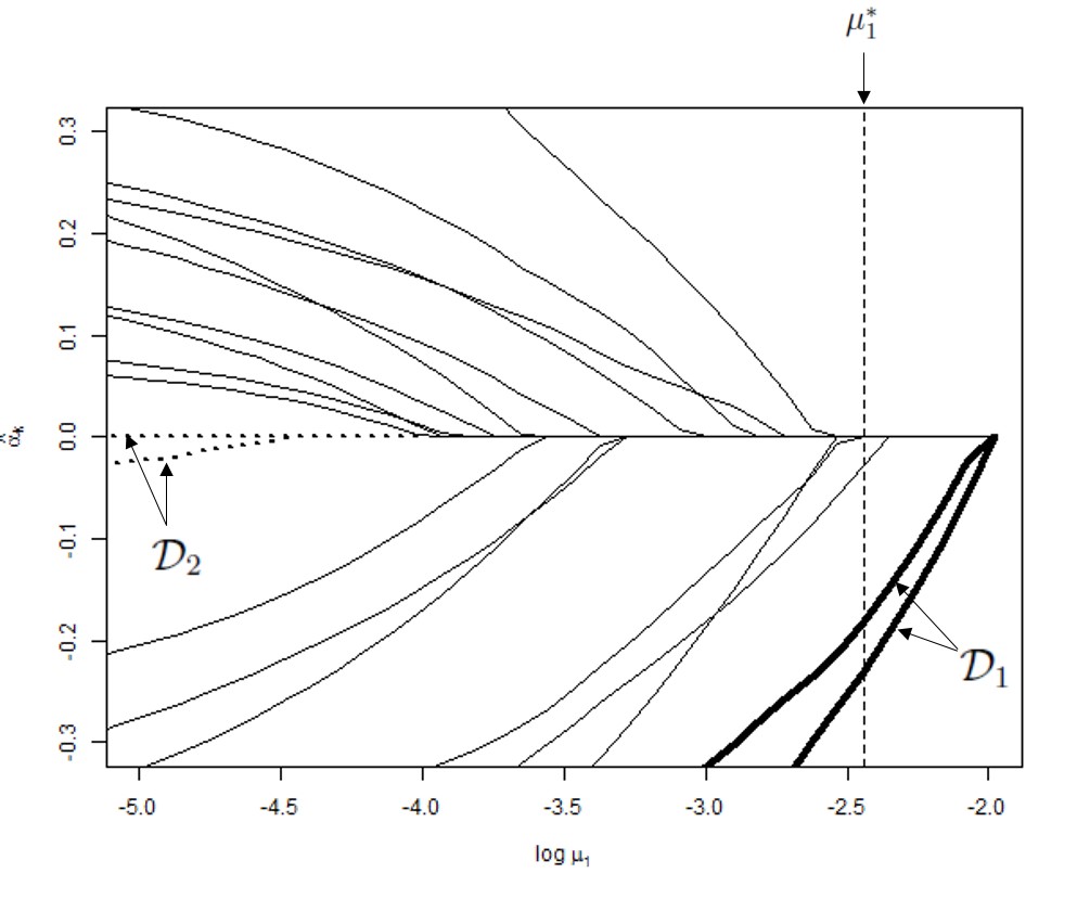
Figure 1: Example of regularization path with $D=20$: $(\hat{\boldsymbol{\alpha}}_{k})_{k=1,\ldots,D}$ are plotted according to different values of the tuning parameter $\mu_{1}$. The vertical dotted line represents the optimal value $\mu_{1}^{*}$ that provides the solutions $(\hat{\boldsymbol{\alpha}}_{k}^{*})_{k=1,\ldots,D}$ of the sparse problem. $(\hat{\boldsymbol{\alpha}}_{k})_{k\in\mathcal{D}_{1}}$ and $(\hat{\boldsymbol{\alpha}}_{k})_{k\in\mathcal{D}_{2}}$ are respectively represented in bold and in pointed lines for $P=0.1$.

Intervals are merged using the following rules:

• “neighbor rule”: consecutive intervals of the same set are merged ($\tau_{k}$ and $\tau_{k+1}$ are merged if both $k$ and $k+1$ belong to $\mathcal{D}_{1}$ or if they both belong to $\mathcal{D}_{2}$) (see a) and b) in Figure 2);

• “squeeze rule”: $\tau_{k}$, $\tau_{k+1}$ and $\tau_{k+2}$ are merged if both $k$ and $k+2$ belong to $\mathcal{D}_{1}$ while $k+1\notin\mathcal{D}_{2}$ (or if both $k$ and $k+2$ belong to $\mathcal{D}_{2}$ while $k+1\notin\mathcal{D}_{1}$) and $l_{k}+l_{k+2}>l_{k+1}$ with $l_{k}=\max\tau_{k}-\min\tau_{k}$ (see c) and d) in Figure 2).

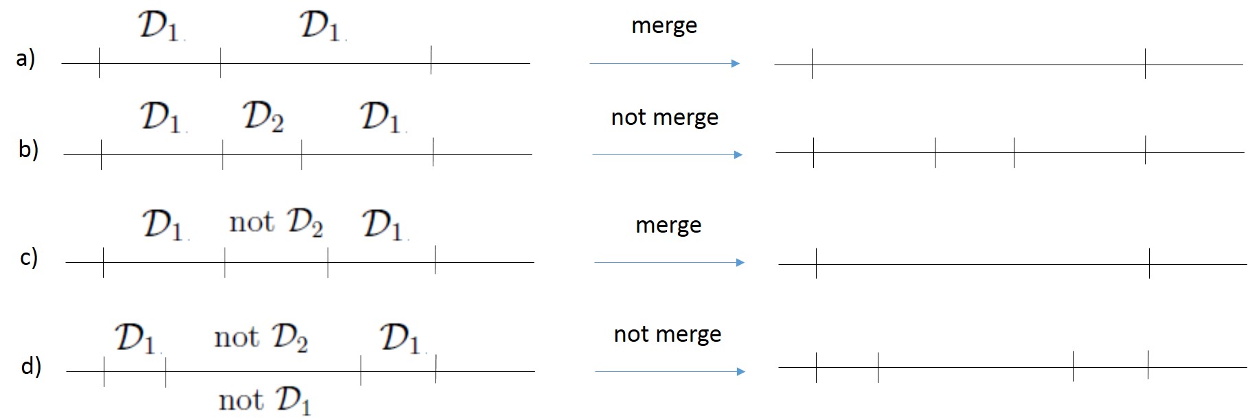
Figure 2: Illustration of the merge procedure for the intervals.

If the current value of $P$ does not yield any fusion between intervals, $P$ is updated by $P\leftarrow P+P_{0}$ in which $P_{0}$ is the initial value of $P$. The procedure is iterated until all the original intervals have been merged.

The result of the method is a collection of models $(\hat{\boldsymbol{\alpha}}_{k}^{*})_{k=1,\ldots,D}$, starting with $p$ intervals and finishing with one. The final selected model is the one that minimizes the CV error. In practice, this often results in a very small number of contiguous intervals which are of the same type (zero or non zero) and are easily interpretable (see Section 6).

Let us remark that the intervals $(\tau_{k})_{k=1,\ldots,D}$ are not used in the ridge step of Section 3.1, which can thus be performed once, independently of the interval search. The whole procedure is described in Algorithm 1.

Algorithm 1 Overview of the complete procedure

1:Ridge estimation

2:Choose $\mu_{2}$ and $d$ according to Section 5

3:Solve the ridge penalized SIR to obtain $\hat{A}$ and $\hat{C}$, ridge estimates of the SIR (see details in Section 3.1)

4:Sparse estimation

5:Initialize the intervals $(\tau_{k})_{k=1,\ldots,D}$ to $\tau_{k}=\{t_{k}\}$

6:repeat

7:     Estimate and store $(\hat{\boldsymbol{\alpha}}_{k}^{*})_{k=1,\ldots,D}$ the solutions of the sparse problem that minimizes the GCV error

8:     Estimate $(\hat{\boldsymbol{\alpha}}_{k}^{+})_{k=1,\ldots,D}$ and $(\hat{\boldsymbol{\alpha}}_{k}^{-})_{k=1,\ldots,D}$ such that at most (resp. at least) a proportion $P$ of the coefficients are non zero coefficients (resp. are zero coefficients), for a given chosen $P$ (details in Section 4)

9:     Update the intervals $(\tau_{k})_{k=1,\ldots,D}$ according to the “neighbor” and the “squeeze” rules (see Section 4)

10:until $\tau_{1}\neq\left[t_{1},t_{p}\right]$

11:Output : A collection of models $(\hat{\boldsymbol{\alpha}}_{k}^{*})_{k=1,\ldots,D}$

12:Select the model $(\hat{\boldsymbol{\alpha}}_{k}^{*})^{*}_{k=1,\ldots,D^{*}}$ that minimizes the CV error

13:Active intervals (for interpretation) are consecutive $\tau_{k}$ with non zero coefficients $\hat{\boldsymbol{\alpha}}^{*}_{k}$

5 Choice of parameters in the high dimensional setting

The method requires to tune four parameters : the number of slices $H$, the dimension of the EDR space $p$, the penalization parameter of the ridge regression $\mu_{2}$ and of the one of the sparse procedure $\mu_{1}$. Two of these parameters, $H$ and $\mu_{1}$, are chosen in a standard way (see Section 6 for further details). This section presents a method to jointly choose $\mu_{2}$ and $d$, for which no solution has been proposed that is suited to our high-dimensional framework. Two issues are raised to tune these two parameters: i) they depend from each other and ii) the existing methods to tune them are only valid in a low-dimensional setting ($p<n$). We propose an iterative method which adapts existing approaches only valid for the low dimension framework and combine them to find an optimal joint choice for $\mu_{2}$ and $d$.

5.1 A Cross-Validation (CV) criterion for $\mu_{2}$

Using the results of Golub et al (1979), Li and Yin (2008) propose a Generalized Cross-Validation (GCV) criterion to select the regularization parameter $\mu_{2}$ and Bernard-Michel et al (2008) explain that this criterion can be applied to their modified estimator, using similar calculations. However, it requires the computation of $\widehat{\Sigma}^{-1/2}$, which does not exist in the high dimensional setting.

We thus used a different strategy, based on $L$-fold cross-validation (CV), which is also used to select the best dimension of the EDR space, $d$ (see Section 5.2). More precisely, the data are split into $L$ folds, $\mathcal{L}_{1}$, …, $\mathcal{L}_{L}$ and a CV error is computed for several values of $\mu_{2}$ in a given search grid and for a given (large enough $d_{0}$). The optimal $\mu_{2}$ is chosen as the one minimizing the CV error for $d_{0}$.

The CV error is computed based on the original regression problem $\mathcal{E}_{1}(A,C)$. In the expression of $\mathcal{E}_{1}(A,C)$ and for the iteration number $l$ ($\in\{1,\ldots,L\}$), $A$ and $C_{h}$ are replaced by their estimates computed without the observations in fold number $l$. Then, an error is computed by replacing the values of $\hat{p}_{h}$, $\overline{X}_{h}$, $\overline{X}$ and $\widehat{\Sigma}$ by their empirical estimators for the observations in fold $l$. The precise expression is given in step 5 of Algorithm  2 in Appendix B.

5.2 Choosing $d$ in a high dimensional setting

The results of CV (i.e., the values of $\mathcal{E}_{1}(A,C)$ estimated by $L$-fold CV) are not directly usable for tuning $d$. The reason is similar to the one developed in Biau et al (2005); Fromont and Tuleau (2006): different $d$ correspond to different MLR (Multiple Linear Regression) problems which cannot be compared directly using a CV error. In such cases, an additional penalty depending on $d$ is necessary to perform a relevant selection and avoid overfitting due to large $d$.

Alternatively, a number of works have been dealing with the choice of $d$ in SIR. Many of them are asymptotic methods (Li, 1991; Schott, 1994; Bura and Cook, 2001; Cook and Yin, 2001; Bura and Yang, 2011; Liquet and Saracco, 2012) which are not directly applicable in the high dimensional framework. When $n<p$, Zhu et al (2006); Li and Yin (2008) estimate $d$ using the number of non zero eigenvalues of $\Gamma$, but their approach requires setting a hyper-parameter to which the choice of $d$ is sensitive. Portier and Delyon (2014) describes an efficient approach that can be used when $n<p$ but it is based on bootstrap sampling and would thus be overly extensive in our situations where $d$ has to be tuned jointly with $\mu_{2}$ (see next section).

Another point of view can be taken from Li (1991) who introduces a quantity, denoted by $R^{2}(d)$, which is the average of the squared canonical correlation between the space spanned by the columns of $\Sigma^{1/2}A$ and the columns of the space spanned by the columns of $\widehat{\Sigma}^{1/2}\widehat{A}$. As explained in Ferré (1998), a relevant measure of quality for the choice of a dimension $d$ is $R(d)=d-\mathbb{E}\left[\mbox{Tr}\left(\Pi_{d}\widehat{\Pi}_{d}\right)\right]$, in which $\Pi_{d}$ is the $\Sigma$-orthogonal projector onto the subspace spanned by the columns of $A$ and $\widehat{\Pi}_{d}$ is the $\widehat{\Sigma}$-orthogonal projector onto the space spanned by the columns of $\hat{A}$. This quantity is equal to $\frac{1}{2}\mathbb{E}\left\|\Pi_{d}-\widehat{\Pi}_{d}\right\|^{2}_{F}$ (in which $\|.\|_{F}$ is the Frobenius norm; see the proof in Appendix A).

In practice, the quantity $\Pi_{d}$ is unknown and $\mathbb{E}\left[\mbox{Tr}\left(\Pi_{d}\widehat{\Pi}_{d}\right)\right]$ is thus frequently estimated by re-sampling techniques as bootstrap. Here, we choose a less computationally demanding approach by performing a CV estimation: $\mathbb{E}\left[\mbox{Tr}\left(\Pi_{d}\widehat{\Pi}_{d}\right)\right]$ is estimated during the same $L$-fold loop described in Section 5.1. An additional problem comes from the fact that, in the high dimensional setting, the $\widehat{\Sigma}$-orthogonal projector onto the space spanned by the columns of $\hat{A}$ is not well defined since the matrix $\widehat{\Sigma}$ is ill-conditioned. This estimate is replaced by its regularized version using the $(\widehat{\Sigma}+\mu_{2}\mathbb{I}_{p})$-orthogonal projector onto the space spanned by the columns of $\hat{A}$ and $\widehat{\Pi}_{d}$ is the $(\widehat{\Sigma}+\mu_{2}\mathbb{I}_{p})$-orthogonal projector onto the space spanned by the columns of $\hat{A}$. Finally, for all $l=1,\ldots,L$, we computed the $(\widehat{\Sigma}^{\setminus l}+\mu_{2}\mathbb{I}_{p})$-orthogonal projector onto the space spanned by the columns of $\hat{A}(l)$ in which $\widehat{\Sigma}^{\setminus l}$ and $\hat{A}(l)$ are computed without the observations in fold number $l$ and averaged the results to obtain an estimate of $\mathbb{E}\left[\mbox{Tr}\left(\Pi_{d}\widehat{\Pi}_{d}\right)\right]$.

In practice, this estimate is often a strictly increasing function of $d$ and we chose the optimal dimension as the largest one before a gap in this increase (“elbow rule”).

5.3 Joint tuning

The estimation of $\mu_{2}$ and $d$ is jointly performed using a single CV pass in which both parameters are varied. Note that only the number of different values for $\mu_{2}$ strongly influences the computational time since SIR estimation is only performed once for all values of $d$, and selecting the first $d$ columns of $\widehat{A}$ for the last computation of the two criteria, the estimation of $\mathcal{E}(A,C)$ and that of $R(d)$. The overall method is described in Appendix B.

6 Experiments

This section evaluates different aspects of the methods on simulated and real datasets. The relevance of the selection procedure is evaluated on simulated and real datasets in Sections 6.1 and 6.3. Additionally, its efficiency in a regression framework is assessed on a real supervised regression problem in Section 6.2.

All experiments have been performed using the R package SISIR. Datasets and R scripts are provided at https://github.com/tuxette/appliSISIR.

6.1 Simulated data

6.1.1 Model description

To illustrate our approach, we first consider two toy datasets, built as follow: $Y=\sum_{j=1}^{d}\log\left|\langle X,\mathbf{a}_{j}\rangle\right|$ with $X(t)=Z(t)+\epsilon$ in which $Z$ is a Gaussian process indexed on $[0,1]$ with mean $\mu(t)=-5+4t-4t^{2}$ and the Matern 3/2 covariance function (Rasmussen and Williams, 2006), and $\epsilon$ is a centered Gaussian variable independent of $Z$. The vectors $\mathbf{a}_{j}$ have a sinusoidal shape, but are nonzero only on specific intervals $I_{j}$: $\mathbf{a}_{j}=\sin\left(\frac{t(2+j)\pi}{2}-\frac{(j-1)\pi}{3}\right)\mathbb{I}_{I_{j}}(t)$.

From this basis, we consider two models with increasing complexity:

• (M1): $d=1$, $I_{1}=[0.2,0.4]$

• (M2): $d=3$ and $I_{1}=[0,0.1]$, $I_{2}=[0.5,0.65]$ and $I_{3}=[0.65,0.78]$.

For both cases the datasets consist of $n=100$ observations of $Y$, digitized at $p=200$ and $300$ evaluation points, respectively. The number of slices used to estimate the conditional mean $\mathbb{E}(X|Y)$ has been chosen equal to $H=10$: according to Li (1991); Coudret et al (2014) among others, the performances of SIR estimates are not sensitive to the choice of $H$, as long as it is large enough (on a theoretical point of view, $H$ is required to be larger than $d+1$).

The datasets are displayed in Figure 3, with a priori intervals provided to test the sparse penalty (see Section 6.1.3 for further details).

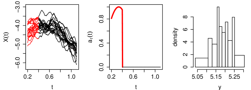
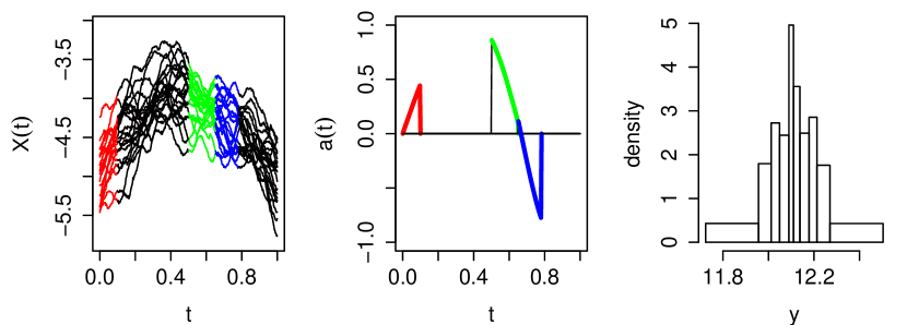
Figure 3: Summary of the two simulated datasets: top (M1), bottom (M2). The left charts display ten samples of $X$, the colors showing the actual relevant intervals; the middle charts display the functions that span the EDR space with the relevant slices highlighted in color; the right charts display the distribution of $Y$.

6.1.2 Step 1: Ridge estimation and parameter selection

The method described in Section 3.1 with parameter selection as in Section 5 has been used to obtain the ridge estimates of $(\mathbf{a}_{j})$ and to select the parameters $\mu_{2}$ (ridge regularization) and $d$ (dimension of the EDR space). Figure 4 shows the evolution of the CV error and of the estimation of $\mathbb{E}(R(d))$ versus (respectively) $\mu_{2}$ and $d$ among a grid search both for $\mu_{2}\in\{10^{-2},10^{-1},...,10^{5}\}$ and $d\in\{1,2,\ldots,10\}$.

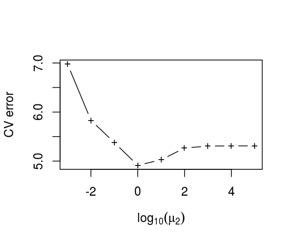
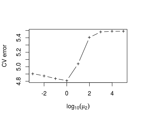
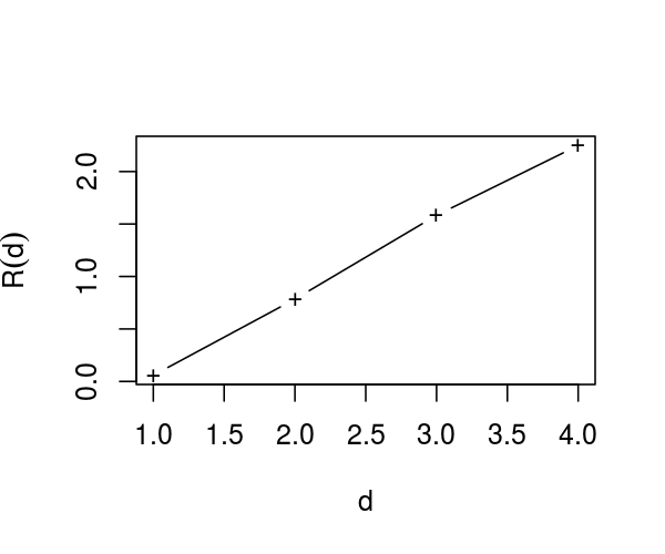
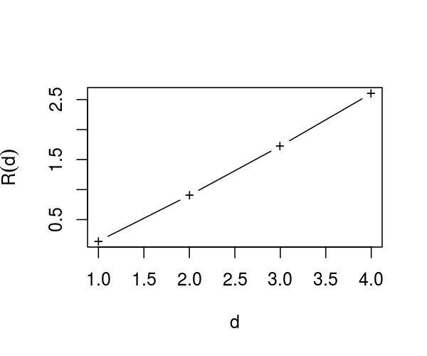
(M1)	(M2)

Figure 4: Top: CV error versus $\mu_{2}$ ($\log_{10}$ scale, for $d=1$) and Bottom: estimation of $\mathbb{E}(R(d))$ versus $d$ (for $\mu_{2}$ = 1 in both cases), for models (M1) (left) and (M2) (right).

The chosen value for $\mu_{2}$ is 1 for both models and the chosen values for $d$, given by the “elbow rule” are $d=1$ for both models. The true values are, respectively, $d=1$ and $d=3$, which shows that the criterion tends to slightly underestimate the model dimension.

6.1.3 Step 2: Sparse selection and definition of relevant intervals

The approach described in Section 4 is then applied to both models. The algorithm produces a large collection of models with a decreasing number of intervals: a selection of the estimates of $\mathbf{a}_{1}$ for (M1), corresponding to those models is shown in Figure 5.

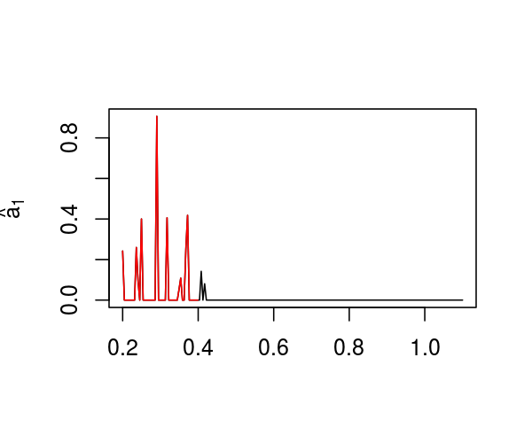
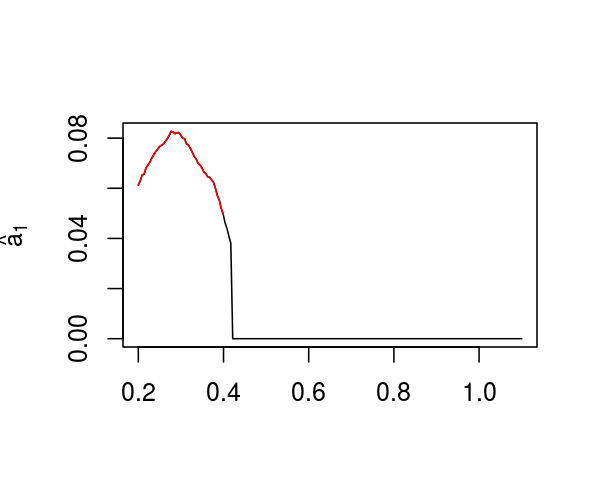
(a) 200 intervals	(b) 142 intervals
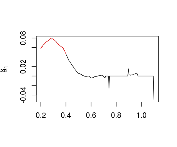
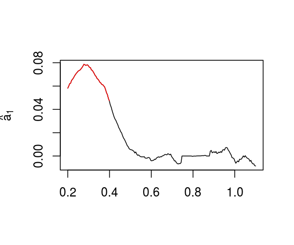
(c) 41 intervals	(d) 5 intervals

Figure 5: (M1) Values of $\hat{\mathbf{a}}_{1}^{s}$ corresponding to four models obtained using the iterative procedure with a different numbers of intervals. (b) is the chosen model and (a) corresponds to a standard sparse estimation with no constraint on intervals.

The first chart (Figure 5,a) corresponds to the standard sparse penalty in which the constraint is put on isolated evaluation points. Even though most of selected points are found in the relevant interval, the estimated parameter $\hat{\mathbf{a}}_{1}^{s}$ has an uneven aspect which does not favor interpretation.

By constrast, for a low number of intervals (less than 50, Figure 5, c and d), the selected relevant points (those corresponding to nonzero coefficients) have a much larger range than the original relevant interval (in red on the figure).

The model selected by minimization of the cross-validation error (Figure 5, b) was found relevant: this approach lead us to choose the model with 142 intervals, which actually correspond to two distinct and consecutive intervals (a first one, which contains only nonzero coefficients and a second one in which no point is selected by the sparse estimation). This final estimation is very close to the actual direction $\mathbf{a}_{1}$, both in terms of shape and support.

The same method is used for (M2). A comparison between the true relevant intervals and the estimated ones is provided in Figure 6 (left).

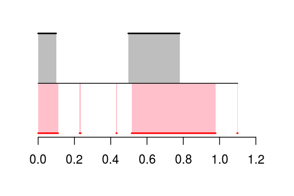
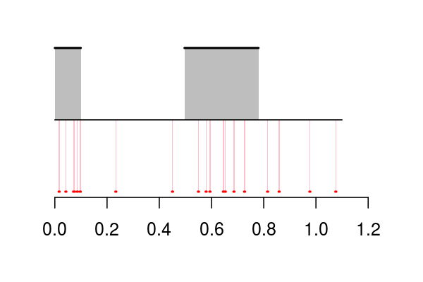
SISIR	standard sparse

Figure 6: (M2) Left: comparison between the true intervals and the estimated ones. True intervals are represented in the upper side of the figure (in black) and by the gray background. Estimated intervals are represented by the red lines in the bottom of the figure and by the pink background. Right: same representation for the standard sparse approach (penalty is applied to $t_{j}$ and not to the intervals).

The support of each of the estimate $\hat{\mathbf{a}}_{1}$ is fairly appropriate: it slightly overestimates the length of the two real intervals and contains only three additional isolated points which are not relevant for the estimation. Compared to the standard sparse approach (right part of Figure 6), the approach is much more efficient to select the relevant intervals and provide more interpretable results by identifying properly important contiguous areas in the support of the predictors.

As a basis for comparison, fused Lasso (Tibshirani et al, 2005), as implemented in the R package genlasso, was used with both (M1) and (M2) datasets. For comparison with our method, we applied fused Lasso on the output of the ridge SIR so as to find $\mathbf{a}_{1}^{s}\in\mathbb{R}^{p}$ that minimizes:

$$\sum_{i=1}^{n}\left[\mathcal{P}_{\hat{\mathbf{a}}_{1}}(X|y_{i})-(\mathbf{a}_{1}^{s})^{\top}\mathbf{x}_{i}\right]^{2}+$$

$$\qquad\lambda_{1}\|\mathbf{a}_{1}^{s}\|_{\ell_{1}}+\lambda_{2}\sum_{j=1}^{p-1}|a_{1j}^{s}-a^{s}_{1,j+1}|,$$

for $\mathbf{a}^{s}_{1}=(a^{s}_{1,1},\ldots,a^{s}_{1,p})$. The tuning parameters $\lambda_{1}$ and $\lambda_{2}$ were selected by 10-fold CV over a 2-dimensional grid search. The idea behind fused Lasso is to have a large number of identical consecutive entries in $\mathbf{a}_{1}^{s}$. In our framework, the hope is to automatically design relevant intervals using this property. Results are displayed in Figure 7 for both simulated datasets.

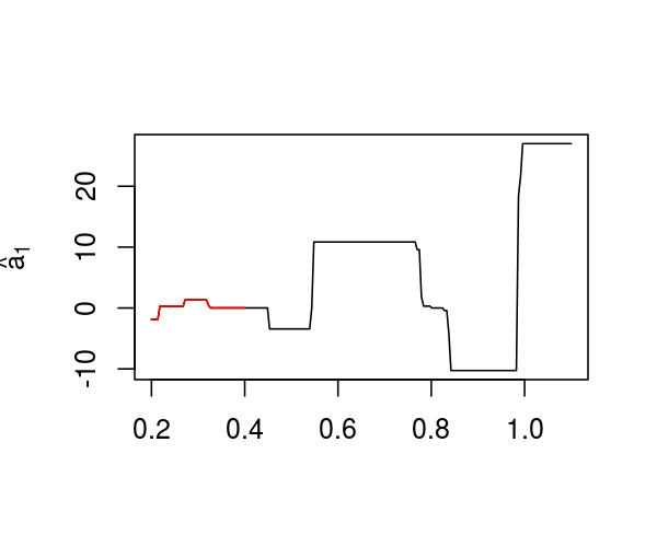
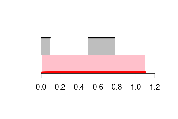
(M1)	(M2)

Figure 7: (M1) Values of $\hat{\mathbf{a}}_{1}^{s}$ obtained with fused Lasso. The target relevant interval is highlighted in red. (M2) Comparison between the true intervals and the estimated ones. True intervals are represented in the upper side of the figure (in black) and by the gray background. Fused Lasso estimated intervals are represented by the red lines in the bottom of the figure and by the pink background.

Contrary to simple Lasso, fused Lasso produces a piecewise constant estimate. However, both for (M1) and (M2), the method fails to provide a sparse solution: almost the whole definition domain of the predictor is returned as relevant.

6.2 Tecator dataset

Additionally, we tested the approach with the well-known Tecator dataset (Borggaard and Thodberg, 1992), which consists of spectrometric data from the food industry. This dataset is a standard benchmark for functional data analysis. It contains 215 observations of near infrared absorbency spectra of a meat sample recorded on a Tecator Infratec Food and Feed Analyzer. Each spectrum was sampled at 100 wavelengths uniformly spaced in the range 850–1050 nm. The composition of each meat sample was determined by analytic chemistry, among which we focus on the percentage of fat content. The data is displayed in Figure 8: the left chart displays the original spectra whereas the right chart displays the first order derivatives (obtained by simple finite differences). The fat content is represented in both graphics by the color level and, as is already well known with this dataset, the derivative is a good predictor of this quantity: these derivatives were thus used as predictors ($X$) to explain the fat content ($Y$).

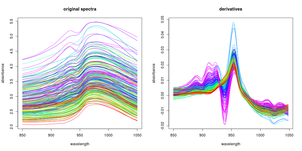
Figure 8: Tecator. 215 near infrared spectra from the “Tecator” dataset (left) and corresponding first order derivatives (right). The color level indicates the percentage of fat content.

We first applied the method on the entire dataset to check the relevance of the estimated EDR space and corresponding intervals in the domain 850–1050 nm. Using the ridge estimation and the method described in Section 5, we set $\mu_{2}=10^{-4}$ and $d=1$.

The relevance of the approach was then assessed in a regression setting. Following the simulation setting described in Hernández et al (2015), we split the data into a training and test sets with 150 observations for the training. This separation of the data was performed 100 times randomly. For each training data set, the EDR space was estimated and the projection of the predictors on this space obtained. A a Support Vector Machine (SVM, $\epsilon$-regression method, package e1071 Meyer et al, 2015) was used to fit the link function $F$ of Equation (1) from both the projection on the EDR space obtained by a simple ridge SIR and the projection on the EDR space obtained by SISIR. The mean square error was then computed on the test set. We found an averaged value equal to 5.54 for the estimation of the EDR space obtained by SISIR and equal to 11.11 when the estimation of the EDR space is directly obtained by ridge SIR only. The performance of SISIR in this simulation is thus half the value reported for the Nadaraya-Watson kernel estimate in Hernández et al (2015).

Even if some methods achieve better performance on this data set (Hernández et al (2015) reported an average MSE of 2.41 for their non parametric approach), our method has the advantage of being easily interpretable because it extracts a few components which are themselves composed of a small number of relevant intervals: Figure 9 shows the intervals selected in the simulation with the smallest MSE, compared to the values selected by the standard Lasso. Our method is able to identify two intervals in the middle of the wavelength definition domain that are actually relevant to predict the fat content (according to the ordering of the colors in this area). On the contrary, standard sparse SIR selects almost the entire interval.

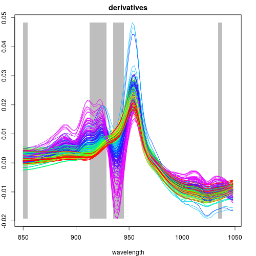
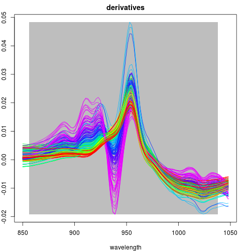
Figure 9: Tecator. Left: original predictors (first order derivatives) with a gray background superimposed to highlight the active intervals found by our procedure. Right: same figure for the standard sparse approach (no constraint on intervals).

6.3 Sunflower yield

Finally, we applied our strategy to a challenging agronomic problem, the inference of interpretable climate-yield relationships on complex crop models.

We consider a process-based crop model called SUNFLO, which was developed to simulate the annual grain yield (in tons per hectare) of sunflower cultivars, as a function of time, environment (soil and climate), management practice and genetic diversity (Casadebaig et al, 2011). SUNFLO requires functional inputs in the form of climatic series. These series consist of daily measures of five variables over a year: minimal temperature, maximal temperature, global incident radiation, precipitations and evapotranspiration.

The daily crop dry biomass growth rate is calculated as an ordinary differential equation function of incident photosynthetically active radiation, light interception efficiency and radiation use efficiency. Broad scale processes of this framework, the dynamics of leaf area, photosynthesis and biomass allocation to grains were split into finer processes (e.g leaf expansion and senescence, response functions to environmental stresses). Globally, the SUNFLO crop model has about 50 equations and 64 parameters (43 plant-related traits and 21 environment-related). Thus, due to the complexity of plant-climate interactions and the strongly irregular nature of climatic data, understanding the relation between yield and climate is a particularly challenging task.

The dataset used in the experiment consisted of 111 yield values computed using SUNFLO for different climatic series (recorded between 1975 and 2012 at five French locations). We focused solely on evapotranspiration as a functional predictor because it is essentially a combination of the other four variables (Allen et al, 1998). The cultural year (i.e., the period on which the simulation is performed) is from weeks 16 to 41 (April to October). We voluntarily kept unnecessary data (11 weeks before simulation and 8 weeks after) for testing purpose (because these periods are known to be irrelevant for the prediction). The resulting curves contained 309 measurement points. Ten series of this dataset are shown in Figure 10, with colors corresponding to the yield that we intend to explain: no clear relationship can be identified between the the value of the curves at any measurement point and the yield value.

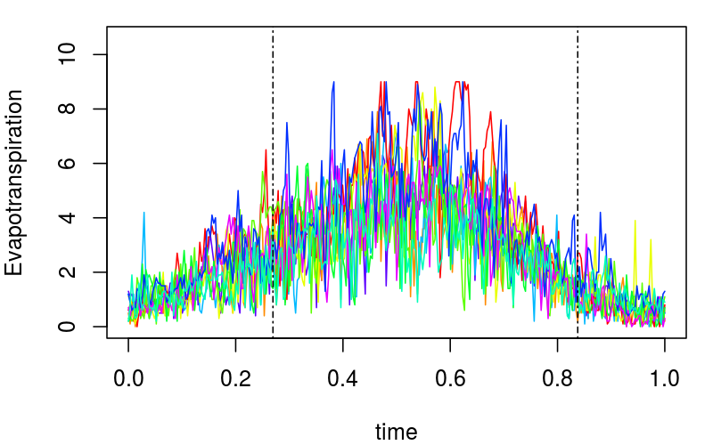
Figure 10: Sunflo. Ten series of evaportranspiration daily recordings. The color level indicates the corresponding yield and the dashed lines bound the actual simulation definition domain.

Using the ridge estimation and the method described in Section 5, we set $\mu_{2}=10^{3}$ and $d=2$. Then, we followed the approach described in Section 4 to design the relevant intervals.

Figure 11 shows the selected intervals obtained after running our algorithm, as well as the points selected using a standard sparse approach. The standard sparse SIR (top of the figure) captures well the simulation interval (with only two points selected outside of it), but fails to identify the important periods within it. In contrast, SISIR (bottom) focuses on the second half of the simulation interval, and in particular its third quarter. This matches well expert knowledge, that reports little influence of the climate conditions at early stage of the plant growth and almost none once the grains are ripe (Casadebaig et al, 2011).

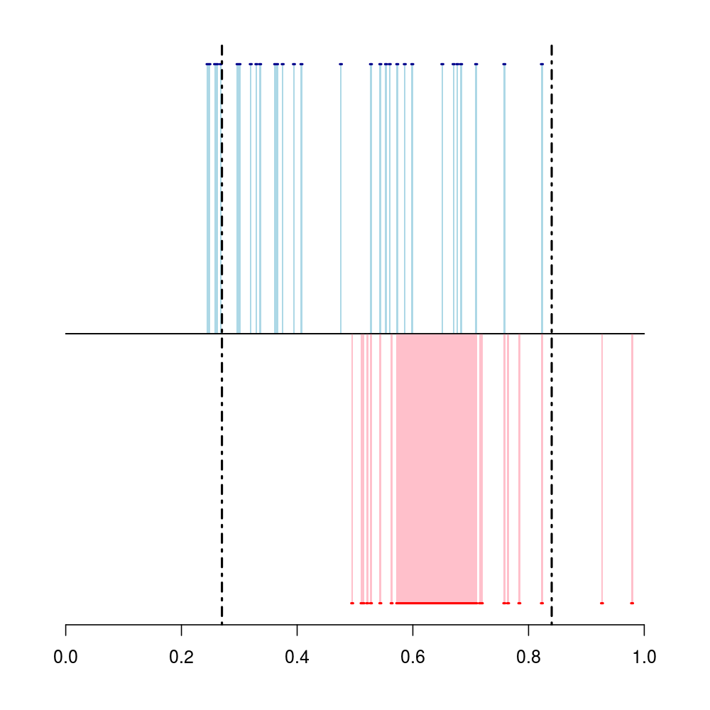
Figure 11: Sunflo. Top: standard sparse SIR (blue). Bottom: SISIR (pink). The colored areas depict the active intervals. The dashed lines bound the actual simulation definition domain.

Appendix A Equivalent expressions for $R^{2}(d)$

In this section, we show that $R^{2}(d)=\frac{1}{2}\mathbb{E}\left\|\Pi_{d}-\widehat{\Pi}_{d}\right\|^{2}_{F}$. We have

$$\frac{1}{2}\left\|\Pi_{d}-\widehat{\Pi}_{d}\right\|^{2}_{F} = \frac{1}{2}\mbox{Tr}\left[\left(\Pi_{d}-\widehat{\Pi}_{d}\right)\left(\Pi_{d}-\widehat{\Pi}_{d}\right)^{\top}\right]$$

$$= \frac{1}{2}\mbox{Tr}\left[\left(\Pi_{d}\Pi_{d}\right)\right]-\mbox{Tr}\left[\left(\Pi_{d}\widehat{\Pi}_{d}\right)\right]+$$

$$\qquad\frac{1}{2}\mbox{Tr}\left[\left(\widehat{\Pi}_{d}\widehat{\Pi}_{d}\right)\right].$$

The norm of a $M$-orthogonal projector onto a space of dimension $d$ is equal to $d$, we thus have that

$$\frac{1}{2}\left\|\Pi_{d}-\widehat{\Pi}_{d}\right\|^{2}_{F}=d-\mbox{Tr}\left[\left(\Pi_{d}\widehat{\Pi}_{d}\right)\right],$$

which concludes the proof.

Appendix B Joint choice of the parameters $\mu_{2}$ and $d$

Notations:

• $\mathcal{L}_{l}$ are observations in fold number $l$ and $\overline{\mathcal{L}_{l}}$ are the remaining observations;

• $\hat{A}(\mathcal{L},\mu_{2},d)$ and $\hat{C}(\mathcal{L},\mu_{2},d)$ are minimizers of the ridge regression problem restricted to observations $i\in\mathcal{L}$. Note that for $d_{1}<d_{2}$, $\hat{A}(\tau,\mu_{2},d_{1})$ are the first $d_{1}$ columns of $\hat{A}(\mathcal{L},\mu_{2},d_{2})$ (and similarly for $\hat{C}(\mathcal{L},\mu_{2},d)$);

• $\hat{p}_{h}^{\mathcal{L}}$, $\overline{X}_{h}^{\mathcal{L}}$, $\overline{X}^{\mathcal{L}}$ and $\widehat{\Sigma}^{\mathcal{L}}$ are, respectively, slices frequencies, conditional mean of $X$ given the slices, mean of $X$ given the slices and covariance of $X$ for observations $i\in\mathcal{L}$;

• $\widehat{\Pi}_{d,\mu_{2}}^{\mathcal{L}}$ is the $(\widehat{\Sigma}^{\mathcal{L}}+\mu_{2}\mathbb{I}_{p})$-orthogonal projector onto the space spanned by the first $d$ columns of $\hat{A}(\mathcal{L},\mu_{2},d_{0})$ and $\widehat{\Pi}_{d,\mu_{2}}$ is $\widehat{\Pi}_{d,\mu_{2}}^{\mathcal{L}}$ for $\mathcal{L}=\{1,\,\ldots,\,n\}$.

Algorithm 2

1:Set $\mathcal{G}_{\mu_{2}}$ (finite search grid for $\mu_{2}$) and $d_{0}\in\mathbb{N}^{*}$ large enough

2:for $\mu_{2}\in\mathcal{G}_{\mu_{2}}$ do

3:     for $l=1,\ldots,L$ do

4:         Estimate $\hat{A}(\overline{\mathcal{L}_{l}},\mu_{2},d_{0})$ and $\hat{C}(\overline{\mathcal{L}_{l}},\mu_{2},d_{0})$

5:         With the observations $i\in\mathcal{L}_{l}$ and for $d\in\{1,\ldots,d_{0}\}$, compute

$$\mbox{CVerr}^{l}_{d,\mu_{2}} = \sum_{h=1}^{H}\hat{p}_{h}^{\mathcal{L}_{l}}\left\|\left(\overline{X}_{h}^{\mathcal{L}_{l}}-\overline{X}^{\mathcal{L}_{l}}\right)-\right.$$

$$\qquad\left.\widehat{\Sigma}^{\mathcal{L}_{l}}\hat{A}(\overline{\mathcal{L}_{l}},\mu_{2},d)\hat{C}_{h}(\overline{\mathcal{L}_{l}},\mu_{2},d)\right\|^{2}_{(\widehat{\Sigma}^{\mathcal{L}_{l}}+\epsilon\mathbb{I})^{-1}}$$

in which $\epsilon$ is a small positive number that makes $(\widehat{\Sigma}^{\mathcal{L}_{l}}+\epsilon\mathbb{I})$ invertible.

6:         For $d\in\{1,\ldots,d_{0}\}$, compute $\widehat{\Pi}_{d,\mu_{2}}^{\overline{\mathcal{L}_{l}}}$

7:         For $d\in\{1,\ldots,d_{0}\}$, compute

$$\hat{R}_{\mu_{2}}(d)=d-\frac{1}{L}\sum_{l=1}^{L}\mbox{Tr}\left(\widehat{\Pi}_{d,\mu_{2}}^{\overline{\mathcal{L}_{l}}}\widehat{\Pi}_{d,\mu_{2}}\right)$$

8:     end for

9:     Compute

$$\mbox{CVerr}_{\mu_{2},d}=\frac{1}{L}\sum_{l=1}^{L}\mbox{CVerr}^{l}_{\mu_{2},d}$$

10:end for

11:State $d^{*}\leftarrow d_{0}$.

12:repeat

13:     Choose $\mu_{2}^{*}=\arg\min_{\mu_{2}\in\mathcal{G}_{\mu_{2}}}\mbox{CVerr}_{\mu_{2},d^{*}}$

14:     Update $d^{*}$ with an “elbow rule” in $\hat{R}_{\mu_{2}^{*}}(d)$

15:until Stabilization of $d^{*}$

16:Output: $\mu_{2}^{*}$ and $d^{*}$

References

- Allen et al (1998) Allen RG, Pereira LS, Raes D, Smith M (1998) Crop evapotranspiration-guidelines for computing crop water requirements-fao irrigation and drainage paper 56. FAO, Rome 300(9):D05,109
- Aneiros and Vieu (2014) Aneiros G, Vieu P (2014) Variable in infinite-dimensional problems. Statistics and Probability Letters 94:12–20
- Bernard-Michel et al (2008) Bernard-Michel C, Gardes L, Girard S (2008) A note on sliced inverse regression with regularizations. Biometrics 64(3):982–986, DOI 10.1111/j.1541-0420.2008.01080.x
- Bettonvil (1995) Bettonvil B (1995) Factor screening by sequential bifurcation. Communications in Statistics, Simulation and Computation 24(1):165–185
- Biau et al (2005) Biau G, Bunea F, Wegkamp M (2005) Functional classification in Hilbert spaces. IEEE Transactions on Information Theory 51:2163–2172
- Borggaard and Thodberg (1992) Borggaard C, Thodberg H (1992) Optimal minimal neural interpretation of spectra. Analytical Chemistry 64(5):545–551
- Bura and Cook (2001) Bura A, Cook R (2001) Extending sliced inverse regression: the weighted chi-squared test. Journal of the American Statistical Association 96(455):996–1003
- Bura and Yang (2011) Bura E, Yang J (2011) Dimension estimation in sufficient dimension reduction: a unifying approach. Journal of Multivariate analysis 102(1):130–142, DOI 10.1016/j.jmva.2010.08.007
- Casadebaig et al (2011) Casadebaig P, Guilioni L, Lecoeur J, Christophe A, Champolivier L, Debaeke P (2011) Sunflo, a model to simulate genotype-specific performance of the sunflower crop in contrasting environments. Agricultural and forest meteorology 151(2):163–178
- Chen and Li (1998) Chen C, Li K (1998) Can SIR be as popular as multiple linear regression? Statistica Sinica 8:289–316
- Chen et al (2015) Chen S, Donoho D, Saunders M (2015) Atomic decomposition by basis puirsuit. SIAM Journal on Scientific Computing 20(1):33–61
- Cook (2004) Cook R (2004) Testing predictor contributions in sufficient dimension reduction. Annals of Statistics 32(3):1061–1092
- Cook and Yin (2001) Cook R, Yin X (2001) Dimension reduction and visualization in discriminant analysis. Australian & New-Zealand Journal of Statistics 43(2):147–199
- Coudret et al (2014) Coudret R, Liquet B, Saracco J (2014) Comparison of sliced inverse regression aproaches for undetermined cases. Journal de la Société Française de Statistique 155(2):72–96, URL http://journal-sfds.fr/index.php/J-SFdS/article/view/278
- Dauxois et al (2001) Dauxois J, Ferré L, Yao A (2001) Un modèle semi-paramétrique pour variable aléatoire hilbertienne. Comptes Rendus Mathématique Académie des Sciences Paris 327(I):947–952, DOI 10.1016/S0764-4442(01)02163-2
- Fauvel et al (2015) Fauvel M, Deschene C, Zullo A, Ferraty F (2015) Fast forward feature selection of hyperspectral images for classification with Gaussian mixture models. IEEE Journal of Selected Topics in Applied Earth Observations and Remote Sensing 8(6):2824–2831, DOI 10.1109/JSTARS.2015.2441771
- Ferraty and Hall (2015) Ferraty F, Hall P (2015) An algorithm for nonlinear, nonparametric model choice and prediction. Journal of Computational and Graphical Statistics 24(3):695–714, DOI 10.1080/10618600.2014.936605
- Ferraty et al (2010) Ferraty F, Hall P, Vieu P (2010) Most-predictive design points for functiona data predictors. Biometrika 97(4):807–824, DOI 10.1093/biomet/asq058
- Ferré (1998) Ferré L (1998) Determining the dimension in sliced inverse regression and related methods. Journal of the American Statistical Association 93(441):132–140, DOI 10.1080/01621459.1998.10474095
- Ferré and Villa (2006) Ferré L, Villa N (2006) Multi-layer perceptron with functional inputs: an inverse regression approach. Scandinavian Journal of Statistics 33(4):807–823, DOI doi:10.1111/j.1467-9469.2006.00496.x
- Ferré and Yao (2003) Ferré L, Yao A (2003) Functional sliced inverse regression analysis. Statistics 37(6):475–488
- Fraiman et al (2016) Fraiman R, Gimenez Y, Svarc M (2016) Feature selection for functional data. Journal of Multivariate Analysis 146:191–208, DOI 10.1016/j.jmva.2015.09.006
- Friedman et al (2010) Friedman J, Hastie T, Tibshirani R (2010) Regularization paths for generalized linear models via coordinate descent. Journal of Statistical Software 33(1):1–22
- Fromont and Tuleau (2006) Fromont M, Tuleau C (2006) Functional classification with margin conditions. In: Lugosi G, Simon H (eds) Proceedings of the 19th Annual Conference on Learning Theory (COLT 2006), Springer (Berlin/Heidelberg), Pittsburgh, PA, USA, Lecture Notes in Computer Science, vol 4005, pp 94–108, DOI 10.1007/11776420˙10
- Fruth et al (2015) Fruth J, Roustant O, Kuhnt S (2015) Sequential designs for sensitivity analysis of functional inputs in computer experiments. Reliability Engineering & System Safety 134:260–267
- Golub et al (1979) Golub T, Slonim D, Wahba G (1979) Generalized cross-validation as a method for choosing a good ridge parameter. Technometrics 21(2):215–223, DOI 10.2307/1268518
- Grollemund et al (2018) Grollemund P, Abraham C, Baragatti M, Pudlo P (2018) Bayesian functional linear regression with sparse step functions, preprint arXiv 1604.08403
- Hastie et al (2001) Hastie T, Tibshirani R, Friedman J (2001) The Elements of Statistical Learning. Data Mining, Inference and Prediction, Springer-Verlag, New York, USA
- Hernández et al (2015) Hernández N, Biscay R, Villa-Vialaneix N, Talavera I (2015) A non parametric approach for calibration with functional data. Statistica Sinica 25:1547–1566, DOI 10.5705/ss.2013.242
- James et al (2009) James G, Wang J, Zhu J (2009) Functional linear regression that’s interpretable. Annals of Statistics 37(5A):2083–2108, DOI 10.1214/08-AOS641
- Kneip et al (2016) Kneip A, Poß D, Sarda P (2016) Functional linear regression with points of impact. Annals of Statistics 44(1):1–30, DOI 10.1214/15-AOS1323
- Li (1991) Li K (1991) Sliced inverse regression for dimension reduction. Journal of the American Statistical Association 86(414):316–342, URL http://www.jstor.org/stable/2290563
- Li and Nachtsheim (2008) Li L, Nachtsheim C (2008) Sparse sliced inverse regression. Technometrics 48(4):503–510
- Li and Yin (2008) Li L, Yin X (2008) Sliced inverse regression with regularizations. Biometrics 64(1):124–131, DOI 10.1111/j.1541-0420.2007.00836.x
- Lin et al (2018) Lin Q, Zhao Z, Liu J (2018) On consistency and sparsity for sliced inverse regression in high dimensions. Annals of Statistics Forthcoming
- Liquet and Saracco (2012) Liquet B, Saracco J (2012) A graphical tool for selecting the number of slices and the dimension of the model in SIR and SAVE approches. Computational Statistics 27(1):103–125
- Matsui and Konishi (2011) Matsui H, Konishi S (2011) Variable selection for functional regression models via the regularization. Computational Statistics and Data Analysis 55(12):3304–3310, DOI 10.1016/j.csda.2011.06.016
- McKeague and Sen (2010) McKeague I, Sen B (2010) Fractals with point impact in functional linear regression. Annals of Statistics 38(4):2559–2586, DOI 10.1214/10-AOS791
- Meyer et al (2015) Meyer D, Dimitriadou E, Hornik K, Weingessel A, Leisch F (2015) e1071: Misc Functions of the Department of Statistics, Probability Theory Group (Formerly: E1071), TU Wien. R package version 1.6-7
- Ni et al (2005) Ni L, Cook D, Tsai C (2005) A note on shrinkage sliced inverse regression. Biometrika 92(1):242–247
- Park et al (2016) Park A, Aston J, Ferraty F (2016) Stable and predictive functional domain selection with application to brain images, preprint arXiv 1606.02186
- Portier and Delyon (2014) Portier F, Delyon B (2014) Bootstrap testing of the rank of a matrix via least-square constrained estimation. Journal of the American Statistical Association 109(505):160–172, DOI 10.1080/01621459.2013.847841
- Rasmussen and Williams (2006) Rasmussen C, Williams C (2006) Gaussian Processes for Machine Learning. The MIT Press, Cambridge, MA, USA
- Schott (1994) Schott J (1994) Determining the dimensionality in sliced inverse regression. Journal of the American Statistical Association 89(425):141–148
- Simon et al (2013) Simon N, Friedman J, Hastie T, Tibshirani R (2013) A sparse-group lasso. Journal of Computational and Graphical Statistics 22:231–245, DOI 10.1080/10618600.2012.681250
- Tibshirani et al (2005) Tibshirani R, Saunders G, Rosset S, Zhu J, Knight J (2005) Sparsity and smoothness via the fused lasso. Journal of the Royal Statistical Society, Series B 67(1):91–108
- Zhao et al (2012) Zhao Y, Ogden R, Reiss P (2012) Wavelet-based LASSO in functional linear regression. Journal of Computational and Graphical Statistics 21(3):600–617, DOI 10.1080/10618600.2012.679241
- Zhu et al (2006) Zhu L, Miao B, Peng H (2006) On sliced inverse regression with high-dimensional covariates. Journal of the American Statistical Association 101(474):360–643