Multiscale approach to equilibrating model polymer melts

Abstract

We present an effective and simple multiscale method for equilibrating Kremer Grest model polymer melts of varying stiffness. In our approach, we progressively equilibrate the melt structure above the tube scale, inside the tube and finally at the monomeric scale. We make use of models designed to be computationally effective at each scale. Density fluctuations in the melt structure above the tube scale are minimized through a Monte Carlo simulated annealing of a lattice polymer model. Subsequently the melt structure below the tube scale is equilibrated via the Rouse dynamics of a force-capped Kremer-Grest model that allows chains to partially interpenetrate. Finally the Kremer-Grest force field is introduced to freeze the topological state and enforce correct monomer packing. We generate $15$ melts of $500$ chains of $10.000$ beads for varying chain stiffness as well as a number of melts with $1.000$ chains of $15.000$ monomers. To validate the equilibration process we study the time evolution of bulk, collective and single-chain observables at the monomeric, mesoscopic and macroscopic length scales. Extension of the present method to longer, branched or polydisperse chains and/or larger system sizes is straight forward.

I introduction

Computer simulations of polymer melts and networks allow unprecedented insights into the relation between microscopic molecular structure and macroscopic material properties such as the viscoelastic response to deformation, see e.g. (Snijkers et al., 2015; Padding and Briels, 2011; Li et al., 2013; Everaers et al., 2004). Such simulation studies rely on very large model systems to reliably estimate material properties, and an important obstacle is the generation of large well equilibrated model systems for long entangled polymer chains.

What do we mean by equilibrium in the case of a linear homopolymer polymer melt? 1) Polymeric liquids have bulk moduli comparable to that of water, and they are nearly incompressible. Hence in equilibrium, we expect model melt states without significant density fluctuations. 2) Single chains in a melt adopt self-similar random walk statistics because excluded volume interactions are screened at length scales sufficiently large compared to monomeric scales. Hence in equilibrium, we expect model states without significant deviations from random walk statistics. 3) At mesoscopic scales, many polymer chains pervade the same volume, such that chains are strongly topologically entangled. This gives rise to the well known plateau modulus.(Doi and Edwards, 1986) Hence in equilibrium, we also require model melts that achieve the correct entanglement density. 4) Finally at the monomeric scale we require the correct monomeric packing, such that we can expect to run long stable simulations where topology is preserved. Taken together, these constraints couple the conformations on scales that range from monomeric to macroscopic length scales. This makes the problem of making equilibrated model melts particular difficult, and the problem is acerbated in the case of heteropolymers or for branched polymers which are of significant industrial interest.

Brute force equilibration of model polymer materials is typically not feasible. Polymer materials display dynamics over a huge range of time scales. Even for polymers of moderate size, their largest conformational relaxation times are many orders of magnitude beyond that which is currently available via brute force simulation. Monomeric motion takes place on pico second time scales, whereas conformational relaxation times can easily reach up to macroscopic time scales. For a long linear polymer chains the dominant relaxation mechanism is reptation(de Gennes, 1971, 1976; Klein, 1978) which gives rise to relaxation times $\tau\sim N^{3}$ where $N$ is the number of monomers.(de Gennes, 1976) In the case of star shaped polymers, reptation is not possible and the dominant relaxation mechanism becomes contour length fluctuations(Zamponi et al., 2005), in which case the relaxation times are $\tau\sim\exp(N_{arm})$, where $N_{arm}$ is the number of monomers in an arm.(Pearson and Helfand, 1984)

To our knowledge, there are three major strategies for equilibrating model polymer melts that address the challenges raised above: a) algorithms that attempts to construct equilibrium model melts with the correct large-scale single chain statistics, b) algorithms that utilize unphysical Monte Carlo (MC) moves to accelerate the dynamics compared to brute force Molecular Dynamics (MD), which simulates the real physical polymer dynamics, c) algorithms using different models e.g. utilizing softer potentials and a push-off process to allow chains to cross to accelerate the relaxation process. In the present approach we combine all these approaches, but before presenting our approach we review examples of these strategies found in the literature.

It is easy to generate single chain conformations with the desired large scale chain statistics. Equilibration procedures following this approach typically place the resulting chains randomly into the simulation domain. However, when monomer packing is introduced, the presence of density fluctuations in the initial state cause significant local chain stretching and compression. Brown et al. (Brown et al., 1994) were the first to recognize the importance of such density fluctuations. This was analyzed in detail by Auhl et al.(Auhl et al., 2003), who made two proposals of how to resolved the density fluctuations, either to accelerate the relaxation utilizing double bridging moves, or to pre-pack the chains in space to avoid density fluctuations. This was done using Monte Carlo simulated annealing and accepting only moves that reduce density fluctuations(Auhl et al., 2003)

An completely different approach is has been proposed by Gao(Gao, 1995). The idea is to start by an equilibrated liquid of monomers and then to create bonds between the monomers corresponding to a melt of polymers. This completely side steps the issue of density fluctuations, since the monomeric liquid is also incompressible. However, the problem becomes how to identify a set of potential bonds to that correspond to a mono-disperse melt of long linear or branched polymers. To reach near complete conversion Gao had to increase the search distance for the last bonds, and to remove the last monomers that could not be bonded. Whereas Gao performed instantaneous bonding on a frozen monomer liquid, Barrat and coworkers(Perez et al., 2008) extended the method by allowing the monomers to move during bonding. This has the effect of enhancing the search distance for bonding. This method still has issues with producing mono-disperse melts, Barrat and coworkers solved the problem by aborting the bonding procedure when 80% of the monomers are linked into mono-disperse chains, and then removing the last 20% of monomers. The resulting states were then compressed to the target pressure, which globally deforms the chain statistics.

Monte Carlo techniques (MC) have the advantage that unphysical moves can be used to accelerate the relaxation dynamics compared to MD techniques, which follow the physical dynamics. A key contribution to the equilibration of polymer melts were the complex MC moves developed by Theodorou and co-workers.(Karayiannis et al., 2002a; Mavrantzas et al., 1999) End-bridging moves works by identifying a the end monomer of one chain and an internal monomer of another chain where the two monomers are in close proximity. The move is performed by cutting the chain at the internal monomer and attaching it to the end of the other chain.(Pant and Theodorou, 1995; Mavrantzas et al., 1999) Double bridging moves works by identifying two pairs of bonded monomers in spatial proximity. The move is performed by replacing the two intramolecular bonds by two intermolecular bonds. The result of these moves is a melt conformation with a new chemical connectivity. Compared with end-bridging moves double-bridging preserves the chain length when equivalent bead pairs along the polymer contours are chosen.

The double bridging moves are the best way currently known to accelerate the polymer dynamics, but method suffers from two major problems: 1) as the chain length is increased the density of potential sites for double bridging drops, and 2) the new proposed connectivity can have a high configurational energy, hence necessitating further tricks to relax the conformation to ensure a reasonable acceptance rate. For instance, it was proposed to reconnect not just monomers, but to grow small bridge segments in order to reduce the conformational energy of the proposed new state.(Karayiannis et al., 2002a) These methods have been used to equilibrate linear melts of polyethylene up to $1000$ monomers(Karayiannis et al., 2002a, b), and polydisperse polyethylene melts up to $5000$ monomers.(Uhlherr et al., 2002) They have also been applied to branched molecules(Karayiannis et al., 2003; Peristeras et al., 2005; Ramos et al., 2007) and grafted polymers(Daoulas et al., 2002, 2003).

The first multi-scale approach was introduced by Subramanian(Subramanian, 2010, 2011), who applied it to linear and branched melts. His idea was to start by equilibrating a coarse representation of the polymer, and successively rescale the simulation domain by while doubling the number of beads in the polymer model. In this way polymer conformations are successively equilibrated on smaller and smaller length scales. A more sophisticated version of hierarchical equilibration has been studied by Zhang et al.(Zhang et al., 2014), where a range of blob chain models were successively fine grained with force field that depended on the scale of fine graining. The most recently proposed equilibration method is that of Moreira et al.(Moreira et al., 2015), who develop the Auhl method further by applying a warm-up procedure where pair-interactions are slowly introduced via a cap on the maximal force as well as the cut-off distance of the pair interactions that is progressively raised using an elaborate feed-back control mechanism during the equilibration process.

Equilibrated melts of atomistic polymer models can be obtained via fine-graining from a coarse-grained polymer model. Theodorou and Suter(Theodorou and Suter, 1985, 1986) studied polymer melts with atomistic models which they prepared by growing atomistic polymer models bond-by-bond in the simulation domain using a metropolis acceptance criterion while taking non-bonded interactions into account when choosing bond angles. The resulting states were then energy minimized. Carbone et al. (Carbone et al., 2010) produce atomistic polymer melts by generating continuous (non-packed) random walks and fine graining them using an atomistic polymer models. For each continuous random walk, a corresponding atomistic polymer chain is created by confining the configuration to follow the continuous random walk, and intra-chain monomeric packing is slowly introduced through a simulation with a soft push-off potential. In a second step, the atomistic polymer chains are placed in the simulation domain, and a second push-off procedure is performed to introduce inter-chain monomeric packing. A similar approach was used by Kotelyanskii et al. but using self-avoiding random walks on a cubic lattice for the initial random walks, which resolves the packing problem.(Kotelyanskii et al., 1996) Recently, Sliozberg et al. equilibrated a one million atom system of polyethylene using an united atom model. (Sliozberg et al., 2016). Similar to Theodorou and Suter the polymers are grown in the simulation domain, taking chemical structure into account to some extend. The resulting melt conformations are then simulated with a soft DPD inspired potential to gentle introduce excluded volume interactions, until they can be switched to the final united-atom force field.

In the present paper, our aim is to present a new general, simple, and computationally effective method of rapidly generating very large equilibrated melts of polymers. We illustrate the method by creating equilibrated monodisperse linear Kremer-Grest (KG)(Grest and Kremer, 1986) polymer models. This polymer model is the standard model for Molecular Dynamics simulations of polymers. The KG model is generic and describes universal polymer properties without attempting to model chemical details of specific polymer species. Chemical details can be introduced in the KG model by varying the effective chain stiffness, which allows us to use this model for studying universal properties of specific polymer types.(Svaneborg et al., 2016) Here we follow Auhl et al.(Auhl et al., 2003) and study how to produce equilibrated melts for a wide range of chain stiffnesses. The typical size of the melts we generate in this study comprise $5-15\times 10^{6}$ beads for chains of $15.000$ beads per chain or $200$ entanglements per chain. These numbers are chosen be about a factor of five above the state of the art e.g. (Zhang et al., 2014; Moreira et al., 2015). However, we are by no means pushing the limitations of the present equilibration approach.

We borrow ideas from many of the approaches described above, but with a few twists and improvements. The most important being that we use different polymer models at the different scales. At the tube length scale, we model the polymer as a chain of entanglement blobs on a lattice and minimize spatial density fluctuations using Monte Carlo simulated annealing. Here we use double-bridge moves, which are easy to identify and always accepted. The lattice conformations are mapped onto a bead-spring model. Subsequently we equilibrate the chain structure at the tube length scale and below using a force capped force field inspired from dissipative-particle dynamics(Hoogerbrugge and Koelman, 1992; Espanol and Warren, 1995). The resulting Rouse dynamics allows chains to pass through each other, and hence equilibrate local chain structure. Finally we switch to the Kremer-Grest force field and thermalize the conformations to produce the correct local bead packing. Each of these steps are fast because we are using computationally efficient models at each scale. The evolution of an example configuration is shown in Fig. 1 for a melt with $M=1.000$ chains of length $N_{b}=15.000$ beads.

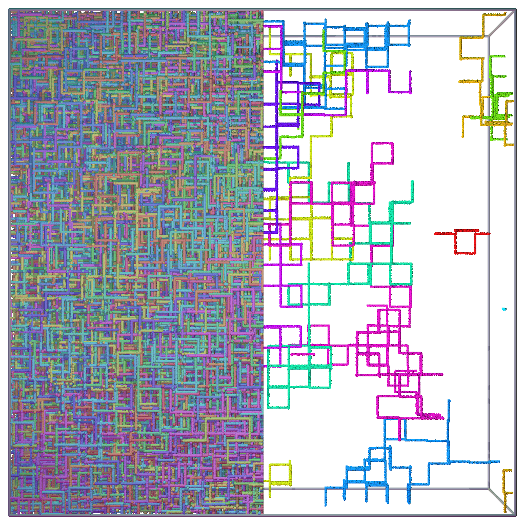
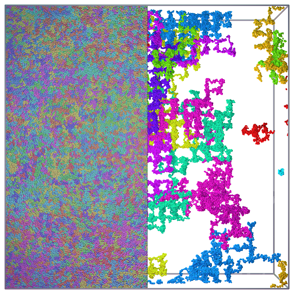
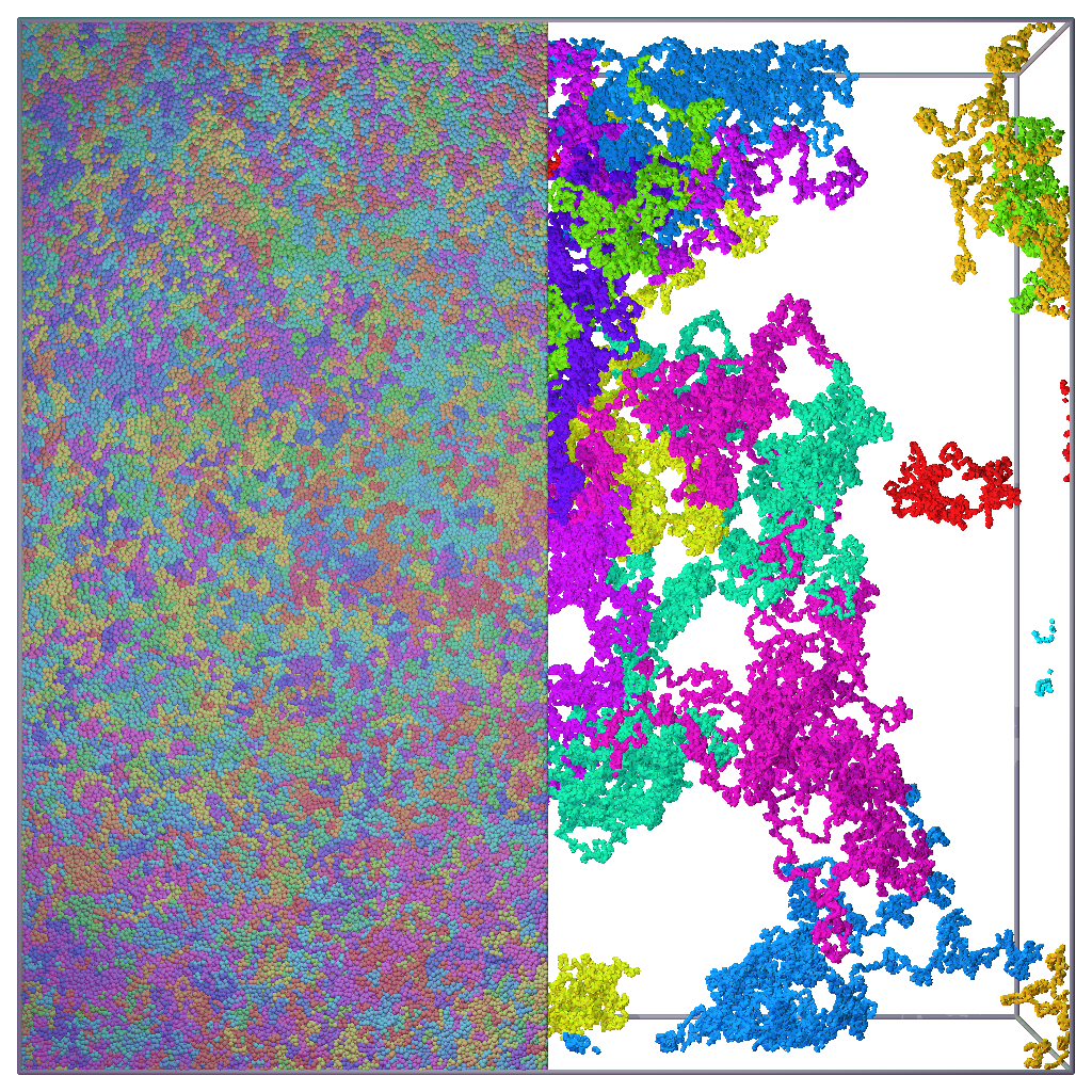
Figure 1: Visualization of a $M\times N_{b}=1.000\times 15.000$ melt state during the equilibration process. All the polymers are shown on the left hand side of the box, while the same $10$ randomly selected polymers are shown on the right hand side of the box. Configuration just after lattice annealing (top left), after $0.1\tau_{e}$ (top right), and $1\tau_{e}$ (bottom left) of Rouse dynamics simulation with the force-capped KG model, and final melt configuration after KG warm up (bottom right).

The paper is structured as follows; In the short theory section we introduce the basic concepts and quantities characterizing polymer melts. In Sect. III, we define and characterize the three polymer models that we use in the paper. In Sect. IV, we proceed to characterize the equilibration process in terms of single-chain, collective, and bulk observables at microscopic, mesoscopic and macroscopic scales. Finally, we conclude with our conclusion in Sect. V.

II Characteristics of polymer melts

Below we introduce the characteristic spatial and temporal scales associated with polymers conformations and their dynamics. At the molecular scale, we can characterize the single chain statistics in a polymer melt as a ideal random walk, since excluded volume interactions are approximately screened.(Flory, 1949; Flory and Jackson, 1989) We can characterize chain statistics either in terms of number of carbon atoms in the backbone or number of monomers, however, since our target here is the Kremer-Grest bead-spring model, we express conformations in terms of the number of beads $N_{b}$ per chain. The end-to-end distance of a chain of $N_{b}$ beads is then given by

$$\langle R^{2}(N_{b})\rangle=c_{b}l_{b}^{2}N_{b}=l_{K}L_{K},$$ (1)

where $l_{b}$ is the average bond length, and $c_{b}$ is the chain stiffness due bead-packing and local chain structure. For $N_{b}\gg 1$ the chain stiffness is given by $c_{b}=\left[\langle\cos\theta\rangle+1\right]/\left[\langle\cos\theta\rangle-1\right]$, where $\theta$ denotes the angle between subsequent bonds. At the Kuhn scale (denoted by subscript “K”) the chain statistics becomes particular simple. It is described by a random walk with contour length $L_{K}=l_{K}N_{K}=l_{b}N_{b}$ where the walk consists of $N_{K}$ Kuhn segments that are statistically independent i.e. $c_{K}=1$ at and above the Kuhn scale.

The Kuhn length can be estimated using

$$l_{K}=\frac{\langle R^{2}(N_{b})\rangle}{L_{K}}=2\sqrt{\langle l_{b}^{2}\rangle}\int_{0}^{N_{b}}\left(1-\frac{n}{N_{b}}\right)C(n)\mbox{d}n,$$ (2)

where we have expressed the mean-square end-to-end distance in terms of the bond correlation function $C(n)=\left\langle{\bf b}(m)\cdot{\bf b}(m+n)\right\rangle_{m}$. This correlation function characterize along how many bonds correlations between bond directions persists. The bond correlation function is easy to sample from simulations.

To define a mesoscopic length scale due to collective chain effects, we can look at most characteristic macroscopic material property of a polymer melt – the plateau modulus. Since polymers can not move though each other, thermal fluctuations are topologically constrained. This leads to a localization of the thermal fluctuations inside a tube-like shape of typical size $d_{T}$.(Edwards, 1967) Each topological entanglement contributes an free energy of $k_{B}T$, and the plateau modulus is the corresponding free energy density

$$G_{N}=\frac{4}{5}\frac{\rho_{K}kT}{N_{eK}}.$$

Here $\rho_{K}=\rho_{b}/c_{b}$ is the number density of Kuhn segments, $\rho_{b}$ the number density of beads, $k$ is the Boltzmann constant, and $T$ the temperature. The entanglement length $N_{ek}$ is a measure of the contour length between topological entanglements along the chain. Note that we specify it in terms of Kuhn units and not beads between entanglements. In the present paper, we generally report results in terms of Kuhn units rather than numbers specific for the Kremer-Grest model. This is to simplify comparisons with theory and experiment, since in Kuhn units we would characterize a real chemical molecule and one of our model molecules with exactly the same numbers independent of the chosen polymer model. The $4/5$ pre-factor is due to the entanglements lost as the stretched chains initially retract into the tube to reestablish their equilibrium contour length.(Doi and Edwards, 1986)

We can relate the length of a tube segment $d_{T}$ to the number of Kuhn units it contains as $d_{T}^{2}=l_{K}^{2}N_{eK}$ and $Z=N_{K}/N_{eK}$ as the number of entanglements/tube segments per chain. Since the tube is a coarse representation of the chain it contains, the large scale tube and chain statistics must coincide, while below the tube length scale, the tube is straight and the chain performs a random-walk. In particular, the chain end-to-end distance matches the end-to-end distance of the tube $\langle R^{2}\rangle=d_{T}^{2}Z=l_{K}^{2}N_{K}$.

The dynamics of short unentangled polymer melts, is described by the Rouse model,(Rouse Jr, 1953; Doi and Edwards, 1986) which also describes the local dynamics of long entangled melts. In this model, a chain is represented by a flexible string of non-interacting units connected by harmonic springs, i.e. each unit represents one Kuhn segment of the polymer. Besides the forces that arise due to connectivity, each unit also receives a stochastic kick and is affected by a friction force, i.e. the Rouse model is endowed with Langevin dynamics. The combined effects of these two forces are to model the presence of the other chains in the melt. The Rouse model can be solved exactly analytically by transforming it to a mode representation, see e.g. (Doi and Edwards, 1986). In particular, the Rouse model predicts the chain centre-of-mass diffusion coefficient $D_{cm}$ and its relation to the Kuhn friction $\zeta_{K}$ as

$$D_{cm}=\frac{kT}{\zeta_{K}N_{K}}.$$ (3)

which has the form of a fluctuation-dissipation theorem. This relation can be inverted to derive the Kuhn friction from a measured diffusion coefficient. The fastest dynamics is that associated with the diffusive motion of individual Kuhn segments one Kuhn length i.e. $\tau_{K}\sim l_{K}^{2}D_{K}^{-1}\sim\zeta_{K}l_{K}^{2}/kT$. A more careful derivation using Rouse theory provides the prefactor as

$$\tau_{K}=\frac{\zeta_{K}l_{K}^{2}}{3\pi^{2}kT}.$$ (4)

In the case of entangled melts, we can define the entanglement time which is the characteristic time it takes an entangled chain segment to diffuse the length of a tube segment $\tau_{e}\sim d_{T}^{2}(D_{K}/N_{e})^{-1}\sim l_{K}^{2}N_{e}^{2}\zeta_{K}/kT$, and with prefactors from Rouse theory

$$\tau_{e}=\tau_{K}N_{e}^{2}=\frac{\zeta_{K}}{3\pi^{2}kT}\frac{d_{T}^{4}}{l_{K}^{2}},$$ (5)

the entanglement time is typically much larger than the fundamental Kuhn time. The conformational relaxation times due to reptation (linear polymers) or contour length fluctuations (star polymers) is again typically much larger than the entanglement time.

The Kuhn length is a microscopic single chain property, and the tube diameter is a collective mesoscale property that is typically associated with pair-wise entanglements.(Everaers, 2012) In order to characterize bulk large scale melt properties and in particular density fluctuations, we use the structure factor. The structure factor is defined as

$$S({\bf q})=\left(N_{b}M\right)^{-1}\left\langle\left|\sum_{j=1}^{M}\sum_{k=1}^{N_{b}}\exp(i{\bf q}\cdot{\bf R}_{jk})\right|^{2}\right\rangle,$$ (6)

where ${\bf q}$ is the momentum transfer in the scattering process. $M$ denotes the number of polymers, and ${\bf R}_{jk}$ the position of the $k$’th bead in the $j$’th polymer. We assume for notational simplicity that all polymers has the same number of beads. When performing simulations with periodic boundary conditions, we are limited to momentum transfers on the reciprocal lattice of the simulation box i.e. ${\bf q}$ vectors of the form ${\bf q}=(2\pi n_{x}/L,2\pi n_{y}/L,2\pi n_{z}/L)$, where $L$ denote the box size. Since the melts are isotropic, we average and bin the structure factor based on the magnitude of the momentum transfer vector denoted $q=|{\bf q}|$. The structure factor for small $q$ values converges to $\lim_{q\rightarrow 0}S(q)=\chi_{T}\rho kT$ where $\chi_{T}$ is the isothermal compressibility of the melt. For a further discussion on density fluctuations and compressibility, we refer to the more detailed derivations in the appendix.

III Polymer models

In the following, we define and characterize the three polymer models employed in the present study: We begin with the Kremer-Grest model (sec. III.1), we also introduce a force capped variant of the Kremer-Grest model (fcKG) (sec. III.2), and finally we introduce a model where chains are modelled as a string of entanglement blobs on a lattice (sec. III.3). We also characterize the Kuhn length for both the KG and fcKG models (sec. III.4), the tube diameter for the Kremer-Grest model (sec. III.5), and finally the Kuhn friction of the fcKG model (sec. III.6). These relations are required to transfer melt conformations between the different polymer models, and to determine how long a Rouse simulation is required for the equilibration process.

III.1 Kremer-Grest polymer model

The end goal of the present equilibration procedure is to produce an equilibrated Kremer-Grest model melt.(Grest and Kremer, 1986; Kremer and Grest, 1990) This is a generic bead-spring polymer model, where all beads interact via a Weeks-Chandler-Anderson (WCA) potential

$$U_{WCA}=4\epsilon\left[\left(\frac{\sigma}{r}\right)^{-12}-\left(\frac{\sigma}{r}\right)^{-6}+\frac{1}{4}\right]\quad\mbox{for}\quad r<2^{1/6}\sigma,$$

while springs are modeled by finite-elastic-non-extensible spring (FENE) potential

$$U_{FENE}=-\frac{kR^{2}}{2}\ln\left[1-\left(\frac{r}{R}\right)^{2}\right],$$

where we choose $\epsilon$ and $\sigma$ as the units of energy and distance respectively. The unit of time is $\tau=\sigma\sqrt{m_{b}/\epsilon}$ where $m_{b}$ denotes the mass of a bead. We add an additional bending interaction given by

$$U_{bend}(\Theta)=\kappa\left(1-\cos\Theta\right).$$

The bending potential was introduced by Faller and MÃŒller-Plathe.(Faller et al., 1999, 2000; Faller and Müller-Plathe, 2001) The KG models are simulated using Langevin dynamics, which couples all beads to a thermostat, and allows long simulations at constant temperature to be performed with reasonable large time steps. The Langevin dynamics is given by the conservative force due pair and bond interactions, as well as a friction term and a stochastic force term:

$$m\frac{\partial^{2}{\bf R}{}_{n}}{\partial t^{2}}=-\nabla_{{\bf R}_{n}}U-\Gamma\frac{\partial}{\partial t}{\bf R}_{n}+{\bf\xi}_{n},$$

where the stochastic force obeys $\langle{\bf\xi}_{n}\rangle=0$ and $\langle{\bf\xi}_{n}(t)\cdot{\bf\xi}_{m}(t^{\prime})\rangle=6kT\Gamma\delta(t-t^{\prime})\delta_{nm}$. The standard choice of the FENE bonds are $R=1.5\sigma$ and $k=30\epsilon\sigma^{-2}$, which produce a bond length of $l_{b}=0.965\sigma$(Subramanian, 2010). Hence the number of beads per Kuhn unit is $c_{b}=l_{K}(\kappa)/l_{b}$. The standard value for the thermostat coupling is $\Gamma=0.5m_{b}\tau^{-1}$. KG model melts are typically simulated with a bead density of $\rho_{b}=0.85\sigma^{-3}$. We use a time step of $\Delta t=0.01\tau$. For integrating the dynamics of our force field, we utilize the GrÞnbech-Jensen/Farago Langevin integration algorithm(Grønbech-Jensen and Farago, 2013; Grønbech-Jensen et al., 2014) implemented in the Large Atomic Molecular Massively Parallel Simulator (LAMMPS).(Plimpton, 1995)

III.2 Force-capped KG model

The KG model preserves topological entanglements via a kinetic barrier of about $75kT$ for chain pairs to move through each other.(Sukumaran et al., 2005) This is due to the strong repulsive pair interaction in combination with a strongly attractive bond potential that diverges when bonds are stretched towards the maximal distance $R$. Preserving topological entanglements is essential for reproducing the plateau modulus. The lattice melt configurations has the correct large scale chain statistics, but as we will show later, the density of entanglements is much too low, hence directly switching from a lattice configuration to a topology preserving KG polymer model would produce model melts with a wrong entanglement density. Hence we need a computationally effective model to introduce the correct random walk statistics inside the tube diameter, and hence produce the correct entanglement density before switching to the KG model.

The force-capped Kremer-Grest model (fcKG) should solve this problem by 1) performing a Rouse like dynamics to introduce local random walk chain statistics, 2) prevent the growth of density fluctuations, 3) avoid the numerical instabilities due to short pair distances or long bonds which can occur in the lattice melt state or during the Rouse dynamics of the fcKG model, and finally 4) approximate the ground state of the KG force field such we can switch to this force field with a minimum of computational effort.

Inspired from dissipative particle dynamics(Hoogerbrugge and Koelman, 1992; Espanol and Warren, 1995) and a previous equilibration methods (Zhang et al., 2014; Moreira et al., 2015), we apply a force-cap to the WCA potential as follows

$$U_{WCA}^{cap}(r)=\begin{cases}(r-r_{c})\left.\frac{dU_{WCA}}{dr}\right|_{r=r_{c}}+U_{WCA}(r_{c})&\quad\quad r<r_{c}\\ U_{WCA}(r)&\quad\quad r_{c}\leq r\leq 2^{1/6}\sigma\\ 0&\quad\quad r>2^{1/6}\sigma\end{cases}.$$ (7)

The inner cutoff distance $r_{c}$ determines the potential at overlap. We choose $U_{WCA}^{cap}(r=0)=5\epsilon$ which corresponds to an inner cutoff of $r_{c}=0.9558\times 2^{1/6}\sigma$. For the bond potential, we choose a fourth degree Taylor expansion of sum of the original WCA and FENE bond potentials around the equilibrium distance ($r_{0}=0.9609\sigma$). The resulting bond potential is

$$U_{bond}(r)=20.2026\epsilon+490.628\epsilon\sigma^{-2}(r-r_{0})^{2}$$

$$-2256.76\epsilon\sigma^{-3}(r-r_{0})^{3}+9685.31\epsilon\sigma^{-4}(r-r_{0})^{4}.$$ (8)

Finally we retain the bending potential

$$U_{bend}(\Theta)=\kappa_{fc}\left(1-\cos\Theta\right),$$

and simulate the fcKG model with exactly the same Langevin dynamics as the full KG model.

We avoid numerical instabilities by using the Taylor expansion in the fcKG model rather than FENE and WCA potentials between bonded beads in the KG model. As a result the numerical stability of the force capped model is considerably improved both for very short and very long bonds. We can simulate the lattice melt states directly (after simple energy minimization) without requiring any elaborate push-off or warm-up procedures to gradually change the force field. Since the force-capped model also approximates the ground state of the full KG model, we can also switch force-capped melt configurations to the full KG force field using simple energy minimization and also avoid designing a delicate push-off or warm-up procedure for this change of force field. Furthermore, expect an increased bead mobility while local single chain structure remains mostly unaffected. Note that in the KG model the WCA interaction is applied between all bead pairs, however for the fcKG model the WCA potential is already included in Taylor expanded bond potential above, hence the pair interaction is limited to non-bonded beads for the force capped KG model.

Figure 2 shows a comparison between the pair and bonded potentials of the KG and fcKG models. The figure also shows the height of the energy barrier of chains passing through each other as function of the force cap expressed as function of the pair potential at overlap $U_{WCA}^{cap}(r=0)$. The transition state is a planar configuration of two perpendicular chains, where two perpendicular bonds open up to allow one chain to pass through the other. Compared to the KG model, this force cap reduce this energy barrier from $75\epsilon$ down to $7.5\epsilon$.

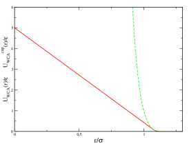
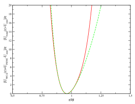
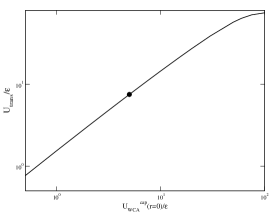
Figure 2: The pair potential (left) and bond potential (middle) for the full KG model (green dashed lines) and for the fcKG model (red solid lines). Shown is also the height of the energetic barrier for chains to pass through each other as function of the force cap (right). The circle denotes our choice of $U_{WCA}^{cap}(r=0)=5\epsilon$

III.3 Lattice blob model

We coarse-grain space into a lattice on a length scale $a$ corresponding to the tube segment length $d_{T}$. The polymers become random walks on this lattice. Since multiple chains pervade an entanglement volume, multiple blobs can occupy the same lattice site. We regard the polymers as consisting of $Z$ entanglement blobs of $N_{e}$ Kuhn segments each. The number of chains within the volume associated with a blob is $n_{e}=\rho_{K}N_{e}^{-1}d_{T}^{3}$. For most flexible well-entangled polymers $n_{e}\sim 19$.(Fetters et al., 2007)

We utilize the recently published lattice polymer model of Wang(Wang, 2009). This model has the computational advantage that the Hamiltonian does not include pair-interactions, which makes it computationally very effective. The Hamiltonian comprises an incompressibility term and a configuration term as follows

$$H=\frac{1}{2\chi\langle n\rangle}\sum_{c}\left(n_{c}-\langle n\rangle\right)^{2}+\sum_{p}\left(\epsilon_{0}N_{p0}+\epsilon_{90}N_{p90}+\epsilon_{180}N_{p180}\right),$$ (9)

the first term is a sum over all sites, while the second is a sum over all polymers. $n_{c}$ denotes the blob occupation number at site $c$, while $\langle n\rangle\approx n_{e}$ is the average number of blobs per site. The parameter $\chi$ plays the role of a compressibility(Helfand and Tagami, 1971, 1972) and hence allows us to introduce incompressibility gradually to remove large scale density fluctuations. In the configuration term we sum over bond angles in the chains. The three terms represents anti-parallel, orthogonal, and parallel successive bonds and their respective energy penalties, respectively. The average bond-bond angle is in this case given by

$$\langle\cos\Theta\rangle=\frac{-\exp(-\beta\epsilon_{0})+\exp(-\beta\epsilon_{180})}{\exp(-\beta\epsilon_{0})+4\exp(-\beta\epsilon_{90})+\exp(-\beta\epsilon_{180})},$$

to obtain non-reversible random walk of blobs we require $\langle\cos\Theta\rangle=0$, such that $c_{L}=\left[\langle\cos\theta\rangle+1\right]/\left[\langle\cos\theta\rangle-1\right]=1$. We choose the parameters $\epsilon_{0}=\epsilon_{180}=1$ and $\epsilon_{90}=0$. We furthermore choose $\chi=1$. Since we are doing simulated annealing the exact values of these parameters are irrelevant. Any state with density fluctuations or configurations with deviations from non-reversible random walks will be exponentially unlikely when the temperature is reduced sufficiently.

We have implemented double bridging, pivot, reptation, and translate moves. Double bridge moves are performed by identifying two pairs of connected blobs on neighboring sites where “crossing over” the bond between the two pairs of blobs does not change mono-dispersity of the melt. Since double bridge moves alters neither angles nor blob positions, the double bridge moves does not change the energy, and are always accepted. Double bridge moves can be carried out both inside a chain and between pairs of chains. Pivot moves picks a random bond and randomly pivots the head or tail of the chain around the the chosen bond.(Madras and Sokal, 1988) Pivot moves only change one angle at the pivot point, but cause major spatial reorganization of the polymer. In densely packed systems, the acceptance rate of pivot moves drops rapidly. Reptation moves delete an number of blobs at either the head or the tail of a polymer and regrows the same number of blobs at the other end of the polymer. Reptation moves are very efficient at generating new configurations in dense systems. Translate moves pick a random bond and randomizes it, and hence randomly translates the head or the tail of the chain by one lattice step relative to the bond. Of the moves discussed here, only the reptation move is limited to linear chain connectivity. We implemented the Metropolis Monte Carlo algorithm in C++ (2011 standard version) making extensive use of standard-template library containers and pointer structures choosing optimal data structures for implementing the infrastructure for generating new moves, rejecting moves with a minimal overhead, and rapidly estimating the energy change of a given trial move.

We note that our choice of lattice length scale $a$ is in fact an arbitrary, since the subsequent Rouse simulation with the fcKG model removes the lattice artifacts. From eq. 5, we see that the Rouse simulations duration growths as the fourth power of the lattice constant. On the other hand, the advantage of enforcing the incompressibility constraint with a lattice Hamiltonian requires a meaningful site occupation numbers $n_{c}\gg 1$. When this limit is approached, the incompressibility constraint converges to an excluded volume constraint and blobs to single monomers. Matching the lattice spacing and the tube diameter producing $\langle n\rangle\sim 19$ offers a reasonable compromise.

III.4 Kuhn lengths of both KG models

In order to have the same chain statistics and in particular a specific Kuhn length for the force capped and full KG models, we need to estimate how these change with stiffness. Theoretically predicting the Kuhn length of a polymer model with pair-interactions is a highly non-trivial problem. While excluded volume interactions are approximately screened in melts (the Flory ideality hypothesis(Flory, 1949; Flory and Jackson, 1989)), melt deviates from polymers in $\Theta$-solutions due to their incompressibility. The incompressibility constraint creates a correlation hole, which leads to a long range net repulsive interaction between polymer blobs along the chain, this effectively causes a renormalization of the bead-bead stiffness to make them stiffer.(Wittmer et al., 2007a, b; Beckrich et al., 2007; Meyer et al., 2008; Semenov, 2010)

To circumvent this problem, we have brute force equilibrated medium length entangled melts with $M=2000$ chains of length $N_{b}=400$ beads while systematically varying the stiffness parameter for both the KG and fcKG models. Each initial melt conformation was simulated for at least $2\times 10^{5}\tau$ while performing double-bridging hybrid MC/MD simulations(Daoulas et al., 2003; Karayiannis et al., 2002b, a, 2003) using the bond/swap fix in LAMMPS(Sides et al., 2004). Ten to twenty configurations from the last $5\times 10^{4}\tau$ of the trajectory were used to estimate the Kuhn length. We choose the chain length as a compromise between having as many Kuhn segments as possible and on having an acceptable double bridging acceptance rate. While double bridging moves are very efficient at removing correlations between the chain conformations, the acceptance rate drops significantly with chain lengths since the potential cross-over points are progressively diluted when requiring that the melt remains mono-disperse. The Kuhn length were derived using eq. 2.

The resulting Kuhn lengths are shown in Fig. 3. As expected, as the stiffness parameter is increased the Kuhn length grows concomitantly. The stiffness of the fcKG and the KG models varies slightly. This is due to the additional stiffness introduced by the WCA pair interaction between next nearest neighbors along the chain compared to the force-capped model. Using the extrapolations shown in Fig 3 we can numerically solve for the force-capped model stiffness $\kappa_{fc}$ required to reproduce equivalent KG model with stiffness parameter $\kappa$. The result is shown in Fig. 3, and is given by the following empirical relationship valid for $\kappa\in[-1:2.5]$.

$$\kappa_{fc}(\kappa)=0.298+0.722\kappa+0.099\kappa^{2}-0.012\kappa^{3}.$$ (10)

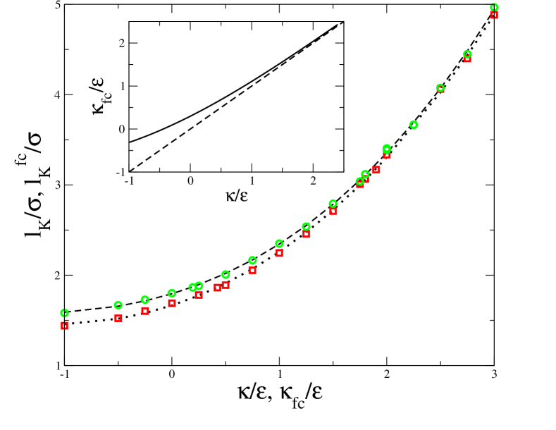
Figure 3: Kuhn length $l_{K}$ vs stiffness parameter for the KG (green circles) and fcKG models (red boxes). The lines are polynomial fits $l_{K}(\kappa)/\sigma=1.795+0.358\epsilon^{-1}\kappa+0.172\epsilon^{-2}\kappa^{2}+0.019\epsilon^{-3}\kappa^{3}$ (hashed black line) and $l_{K}^{fc}(\kappa_{fc})/\sigma=1.666+0.389\epsilon^{-1}\kappa_{fc}+0.192\epsilon^{-2}\kappa_{fc}^{2}+0.012\epsilon^{-3}\kappa_{fc}^{3}$ (dotted black line). The insert shows the relation between $\kappa_{fc}$ and $\kappa$ defined by eq. 10. (solid black line)

III.5 Tube diameter of Kremer-Grest melts

In order to choose the spacing of the lattice model, we need to estimate the length of a tube segment $a(\kappa)$ as function of stiffness $\kappa$ for the KG model. We have generated $15$ melt states with $M=500$ chains of length $N_{b}=10.000$ for $\kappa=-1,-0.75,-0.50,\cdots,2.25,2.50$. We used the algorithm of the present paper, but chose the lattice spacing $a=l_{K}(\kappa)\sqrt{N_{K}(\kappa)}$, with $N_{K}(\kappa)=100c_{b}^{-1}(\kappa)$. This corresponds to using not entanglement blobs, but rather blobs with a fixed number of beads ($100$) independently of chain stiffness.

We have performed primitive-path analysis (PPA) of the melt states.(Everaers et al., 2004) During the PPA a melt conformation is converted into the topologically equivalent primitive-path mesh-work characterizing the tube structure. We have performed a version of the PPA analysis which preserves self-entanglements by only disabling pair interactions between beads within a chemical distance of $2c_{b}N_{eK}$ bonds.(Sukumaran et al., 2005) The minimization was performed using the steepest descent algorithm implemented in LAMMPS followed by dampened Langevin dynamics as described in Ref. (Everaers et al., 2004).

Since the large scale chain melt statistics and primitive-path statistics agree, the PPA essentially consists of filtering out the effects of thermal fluctuations on the chain configurations. The chain mean-square end-to-end distance is constant, and hence the Kuhn length of the tube (the tube diameter) is given by $a=\langle R^{2}\rangle/L_{pp}$. $L_{pp}$ is the average primitive-path contour length, which we obtain directly from the mesh work produced by the PPA. By preforming the analysis on melts of varying $\kappa$ we can obtain the tube diameter as function of chain stiffness $a(\kappa)$. The result is shown in Fig. 4, and as expected, when the chains becomes stiffer they can pervade a large volume and hence become more entangled, which corresponds to the observed decrease of the tube diameter. The generated melts range from $Z(\kappa=-1)=80$ to $Z(\kappa=2.5)=540$ entanglements. Hence, they are all deep inside the regime of strongly entangled polymer melts, where we can neglect the effect of ends during the PPA process.(Hoy et al., 2009)

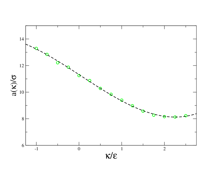
Figure 4: Tube segmental length $a(\kappa)$ vs stiffness parameter for the KG model (green symbols), also shown is an interpolation given by $a(\kappa)/\sigma=11.32-2.096\epsilon^{-1}\kappa-0.0293\epsilon^{-2}\kappa^{2}+0.1465\epsilon^{-3}\kappa^{3}$

III.6 Time mapping of the force-capped KG model

In order to estimate how long time we should run the Rouse simulation to relax chain statistics up to the tube scale, we need to know the entanglement time of the fcKG model. The unit of time of the simulated force field is $\tau$, however, this unit has no direct relation to the time scales characterizing the emergent polymer dynamics, which depends on the force field as well as the thermostat parameters. To define a natural time scale for the polymer dynamics, we obtain the effective Kuhn friction $\text{$\zeta$}_{K}$. We have measured the center-of-mass (CM) diffusion coefficient by performing a series of simulations with varying stiffness parameter $\kappa_{fc}$. Each melt contains $2.000$ molecules and chain length $N_{K}=10,20,30,40$. The melts were equilibrated for a period of $10^{4}\tau$ using double bridging hybrid MC/MD(Daoulas et al., 2003; Karayiannis et al., 2002b, a, 2003). The resulting equilibrium states were run for up to $2-10\times 10^{5}\tau$ and the center of mass diffusion coefficient $D_{cm}(\kappa_{fc},N_{K})$ was obtained from the plateau of the measured mean-square displacements $D_{cm}(\kappa_{fc},N_{K};t)=\langle[R_{cm}(t)-R_{cm}(0)]^{2}\rangle/[6t]$ for $t>10^{5}\tau$ by sampling plateau values for log-equidistant times, and discarding simulations where the standard deviation of the samples exceeded $2\%$ of their average value.

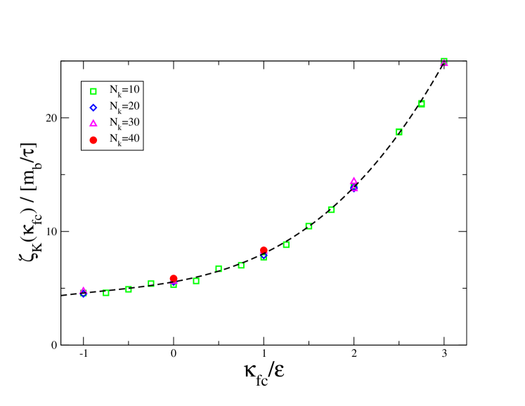
Figure 5: Kuhn friction for the fcKG model as function of stiffness parameter $\kappa_{fc}$. The line through the data points is the fit $\zeta(\kappa_{fc})/[m_{b}/\tau]=5.5657+1.4367\epsilon^{-1}\kappa_{fc}+0.7564\epsilon^{-2}\kappa_{fc}^{2}+0.30372\epsilon^{-3}\kappa_{fc}^{3}$.

Figure 5 shows the Kuhn friction obtained from the analysis of the simulations using eq. 3. We observe that the friction increases slowly with chain stiffness. The excellent collapse of data from different chain lengths supports the validity of the Rouse dynamics for the force-capped KG model.

Using Eq. 5 and the empirical relations shown in Figs. 4, 3, and 5, we obtain an empirical relation for the entanglement time of the fcKG model as

$$\tau_{e}(\kappa_{fc})/\tau=935.5-710.8\epsilon^{-1}\kappa_{fc}+226.6\epsilon^{-1}\kappa_{fc}^{2}-26.61\epsilon^{-1}\kappa_{fc}^{3},$$ (11)

valid within the range of $\kappa_{fc}=-1,\dots,2.5$. The entanglement time varies from $1900\tau$ down to $160\tau$ as chains gets stiffer. For simplicity, we define $\tau_{e}(\kappa)\equiv\tau_{e}(\kappa_{fc}(\kappa))$ below to simplify the notation. This does not lead to confusion since in the present paper entanglement times always refers to the Rouse simulations of the force capped model, and the aim of running a fcKG model to equilibrate the corresponding KG models with a specific stiffness $\kappa$.

Figure 6 shows the mean-square displacements $MSD(t)=\langle[{\bf R}_{i}(0)-{\bf R}_{i}(t)]^{2}\rangle$ of beads for the fcKG and KG models. We observe the expected sub-diffusive Rouse power law $MSD(t)\sim t^{1/2}$ both above and below the estimated entanglement for the fcKG model, whereas for the KG model we see the start of the crossover to a $MSD(t)\sim t^{1/4}$ power law above the entanglement time. The latter dynamics is due to local reptation motion inside the tubes. This observation is consistent with our assumption that the fcKG model produces Rouse dynamics because it allows chains to pass through each other. Hence the entanglement Rouse time of the fcKG model is the relevant time for establishing local random walk structure inside the tube. The mean-square displacements for the KG models were shifted using the Kuhn times for the corresponding fcKG models in order to retain the horizontal shift between the curves. This shift indicates that the dynamics of the full KG model is approximately a factor of six slower than the fcKG model. We have used this factor to estimate the entanglement times for the full KG model, which are also shown in the figure and is in good agreement with the indicated power law cross-overs.

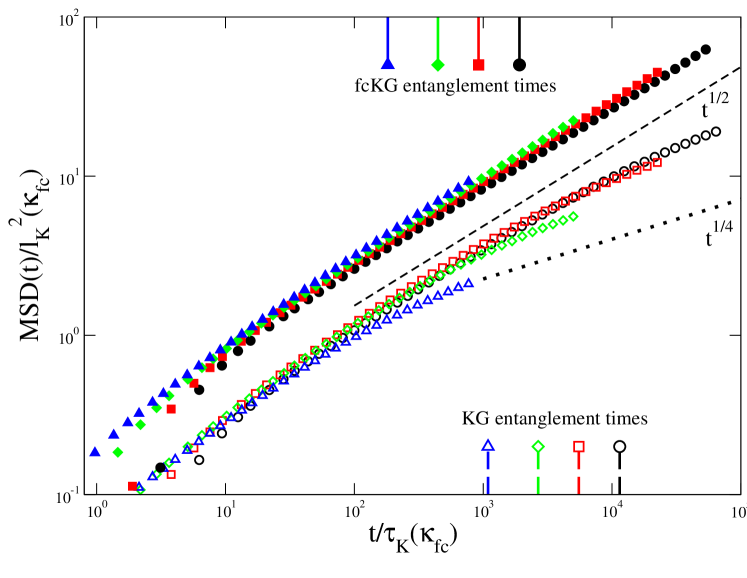
Figure 6: Mean-square displacements for the fcKG model (filled symbols) and KG model (open symbols) for melts with $M\times N_{b}=500\times 10.000$ for $\kappa,\kappa_{fc}=-1$ (black circle), $0$ (red box), $1$ (green diamond), and $2$ (blue triangle up). For the KG model the times were normalized using the time mapping for the corresponding force-capped KG model to retain their horizontal position. Also indicated are the entanglement times for the fcKG model and estimated for the KG model (vertical lines ending a single symbol of the corresponding model).

III.7 Switching between models

Using the relations derived above we can fine-grain melt states from the lattice model to the fcKG model, and later introduce the target KG model and retaining the desired melt properties through the whole equilibration process.

After lattice annealing of large scale density fluctuations, the final lattice polymer melt state is converted into an off-lattice bead-spring model representation, that can be used as input for the subsequent Molecular Dynamics simulations. Each lattice chain is translated in space by a random vector in a cell $[-a/2,a/2]^{3}$, and decorated with beads to produce the desired target contour length density of beads. Each bead is furthermore offset by a small random vector in $[-a/200,a/200]^{3}$ to facilitate energy minimization. This melt shown in Fig. 1 corresponds to a $23\times 23\times 23$ lattice, and each polymer chain consists of $200$ entanglement blobs.

After the lattice annealing, the Rouse simulation should introduce random chain structure at progressively larger and larger scales. Before starting the Rouse simulation, the energy of the final lattice conformation is minimized with the force-capped force field. The melt configuration after $0.1\tau_{e}$ is shown in Fig. 1. After $0.1\tau_{e}$ the lattice structure is still visible. However, after $1\tau_{e}$ of Rouse simulation the polymers appears to have adopted a random walk conformation on the tube scale, and no signs of the lattice structure remains. After having simulated Rouse dynamics with the fcKG model for a number of entanglement times $\tau_{e}$, we expect that the correct chain statistics have been established on all scales.

To switch a fcKG melt conformation to the KG force field, it is first energy minimized using the full WCA pair interaction, but retaining the fcKG bond potential. Subsequently, the bond potential is changed to sum of the FENE and WCA potentials and again the energy is minimized. The resulting melt conformation is then simulated for $5\times 10^{4}$ MD steps at $T=1\epsilon$ with the full KG force field to equilibrate the local bead packing. We denote this procedure the KG warm-up. The resulting KG configuration is also shown in Fig. 1. It shows no discernible difference compared to the fcKG melt state at $1\tau_{e}$.

IV Characterization of equilibration process

Above, we characterized the KG and fcKG models using results for $15$ melt states of $M\times N_{b}=500\times 10.000$ i.e. $Z=80,\dots,540$ entanglements for $\kappa=-1,-0.75,-0.50,\cdots,2.25,2.50$. We have also equilibrated a number of large melts with $M\times N_{b}=1.000\times 15.000$ i.e. $Z=200$ but only in the case of $\kappa=0$. In comparison, the largest melts produced in Refs. (Moreira et al., 2015; Zhang et al., 2015) where $1.000$ chains of length $2.000$ beads. We produced eight melts using the full lattice Hamiltonian described above, five melts without the incompressibility term, and three melts without the configuration term. With these variations of the annealing procedure, we can illustrate why both the incompressibility and configuration terms are required. The lattice states were simulated with the same Rouse simulation, but we have also performed the KG warm up at different times during the Rouse simulation to study how this impacts the resulting KG melts. Below we will characterize the $1.000\times 15.000$ melts states unless specifying a chain stiffnesses $\kappa$, in which case the observables are calculated for the $500\times 10.000$ melt states.

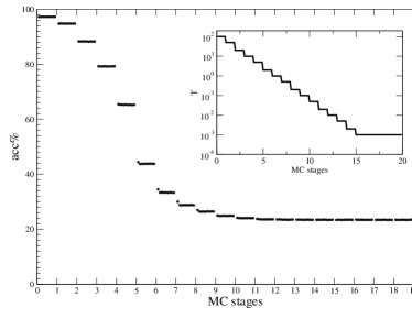
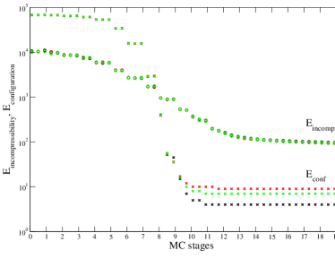
Figure 7: Characterization of simulated annealing process showing total acceptance probability (right) and energy contributions from configuration (circles) and incompressibility (crosses) terms for three melts (red, green, black). The insert shows the temperature profile.

Figure 7 shows a characterization of the simulated annealing process. After some experimentation, we chose an annealing protocol where the temperature is reduced in $20$ annealing stages from $T=10^{2}$ to $10^{-3}$. At each annealing stage, we attempt $50$ Monte Carlo (MC) moves per blob in the melt, where we use both global and local Monte Carlo moves. Above the transition temperature $T^{*}\sim 0.1$, the system rapidly equilibrates and the acceptance probability shows a clear step structure. Below the transition temperature, the equilibration slows down considerably and the step like structure of the acceptance probability is lost. The acceptance rate remains clearly above $20\%$ even below the transition temperature. This is primarily due to the end-bridging moves, which are attempted with $20\%$ probability. The local chain dynamics becomes frozen while the global chain state remains dynamic, since double bridge moves are still accepted with even below the transition temperature. Figure 7 also shows the decrease of the energy contributions from the incompressibility and configuration terms in the lattice Hamiltonian. The configuration energy contribution drops by about four orders of magnitude while the incompressibility energy drops by about two orders of magnitude. Both contributions levels out after $10-12$ annealing stages. After this time, the three melts have reached approximately the same energy minimum.

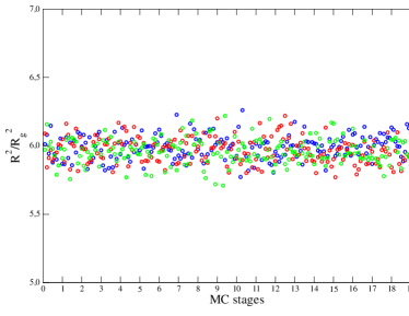
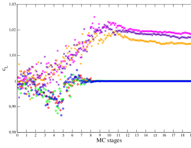
Figure 8: Melt characterization during simulated annealing showing $\langle R^{2}\rangle/\langle R_{g}^{2}\rangle\approx 6$ ratio (left) and chain stiffness $c_{L}$ for lattice melts with the configuration term (red, green, blue circles) and without the configuration term in the Hamiltonian (magenta, orange, purple crosses).

Figure 8 shows how the chain conformations evolve during the annealing process. We describe the large scale properties with the ratio of the end-to-end distance and the radius of gyration which for a random walk should be about six.(Flory and Jackson, 1989) We observe that at large scales the melt conformations remain random walk like during the whole annealing process. Furthermore the scatter of the curves below the transition temperature again shows that the MC moves keeps generating new conformations searching for a better minimum.

The chain stiffness $c_{L}$ characterizes blob chain angle statistics at the tube scale. This should be unity for random walks where subsequent steps are statistically uncorrelated. For melts with the configuration term, this is seen to be the case after some transients around the transition temperature, however, we see a slight but systematic increase in the chain stiffness for melts without the configuration term. This could be either due to the incompressibility constraint acting as a weak excluded volume even at occupation numbers of $\langle n\rangle\approx 19$, and hence leading to a small degree of swelling. Alternatively, it is also known that the Flory ideality hypothesis is only approximately true even for dense melts. The incompressibility constraint leads to a correlation hole of density fluctuations, which has been shown to give rise to an effective weakly repulsive intra-molecular interaction.(Wittmer et al., 2007a, b; Beckrich et al., 2007; Meyer et al., 2008; Semenov, 2010) Both these effects lead to swelling, and the severity of the swelling is likely to depend on the rate at which the simulated annealing process is quenched. We have opted for adding the additional configuration term to the lattice Hamiltonian, to ensure that the lattice conformations show the desired random walk statistics at the smallest scales.

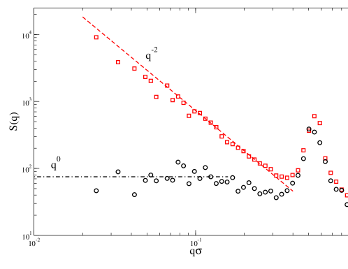
Figure 9: Structure factor for initial lattice configurations with density fluctuations (red boxes), and after simulated annealing with the incompressibility term (black circles). Also shown are the power laws expected from the density fluctuations and from incompressibility (hashed and dash-dotted lines)

Figure 9 shows the impact of incompressibility on the lattice melt conformations. We have averaged the structure factor over several statistically independent melts to improve the statistics. At the lowest $q$ values, the structure factor characterize density fluctuations on the scale of the whole simulation domain, whereas the highest $q$ values reflect density fluctuations on the scale of individual blobs. The structure factors were calculated for MD bead-spring melt states and include effects due to random shifts of chains and beads described above.

For the lattice simulations without the incompressibility term, very large scale density fluctuations can be seen at large scales, which follows the predicted power law behavior $S(q)\sim 2N_{b}(qR_{g})^{-2}$ (for derivation see the Appendix). This power law reflects the density fluctuations created by randomly inserting the polymer chains on the lattice. After annealing, with the the incompressibility term in the Hamiltonian the large scale density fluctuations are reduced by about two orders of magnitude, and the resulting structure factor is flat indicating constant density on all scales as expected for an incompressible melt. A large peak is seen in both the lattice configurations, this peak reflects the lattice structure and the position is given by $q_{lattice}=2\pi/a$.

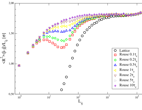
Figure 10: Evolution of mean-square internal distances during equilibration for the initial lattice configuration (black circle), and after $0.1\tau_{e}$, $0.2\tau_{e},0.5\tau_{e},1\tau_{e}$, $2\tau_{e}$, $5\tau_{e}$, $10\tau_{e}$, $20\tau_{e}$ of Rouse simulation time with the fcKG for $\kappa=0$.

Figure 10 shows the evolution of single chain conformations characterized by their mean-square internal distances (MSID), which are defined by $MSID(L_{ij})=\langle({\bf R}{}_{i}-{\bf R}{}_{j})^{2}\rangle/L_{ij}$ where ${\bf R}{}_{i}$ is the position of the $i$’th bead on a chain, and $L_{ij}=l_{b}|i-j|$ denotes the chemical contour length between the two beads. For large chemical distances the MSID converges to the Kuhn length, whereas for neighboring monomers it is identical to the bond length $l_{b}$. Between these limits it characterize the local effects of the chain stiffness.

The evolution of the chain statistics during the Rouse simulation is shown in Fig. 10. The final state from the lattice simulation matches the large scale chain statistics by construction, but shows strong compression at all length scales below the tube diameter, which is an expected lattice artifact. After energy minimization and a brief simulation, the bond distance agrees with the KG model, but chains are stretched at very short scales, and compressed at scales all the way to the tube scale. During the Rouse simulation, the chain statistics is progressively equilibrated at intermediate scales such that the desired chain statistics is established on all length scales. In the initial lattice configuration all the beads are lying on a straight line and hence we approach the equilibrium chain statistics from below, whereas in the approach of Auhl et al.(Auhl et al., 2003), their push off produced a peak in the MSID that is due to local chain stretching due to density fluctuations, which was mitigated by the introduction of a pre-packing procedure. Here our fcKG model has been designed to perform this pre-packing on scales below the tube diameter during the Rouse simulation.

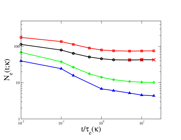
Figure 11: Topological evolution of the melt during the Rouse simulation. The entanglement lengths of the force-capped KG model melts for $\kappa=-1\epsilon$ (red box), $0\epsilon$ (black circle), $1.5\epsilon$ (green diamond), and $2.5\epsilon$ (blue triangle up). Also shown are the entanglement length of melts after the KG warm up for three different times along the Rouse simulation for $\kappa=0\epsilon$ (red crosses).

The MSID is a single chain observable, we can also take melt configurations at various times along the Rouse dynamics simulation and submit them to PPA analysis to estimate the topological evolution of the melt. The entanglement length has been shown to be quite sensitive to the equilibration procedure, since chain stretching during equilibration of badly prepared samples artificially increase the entanglement density.(Hoy and Robbins, 2005) The result is shown in Fig. 11. The entanglement length is seen to systematically decrease towards the equilibrium entanglement length after about one entanglement time of Rouse dynamics independently of chain stiffness. During the Rouse simulation chains can pass through each other, however, during the PPA the topological structure is frozen. Hence the figure shows the growth of the entanglement density due to the random chain structure that is gradually introduced by the Rouse dynamics of the fcKG model. The figure also shows that the initial lattice states produce a completely wrong entanglement density, hence any attempt to equilibrate it with a topology preserving chain model would fail. Finally, the entanglement length of the three conformations after the KG warm up are in excellent agreement with that of the Rouse simulations, as expected the KG warm up does not change the topological structure of the melts.

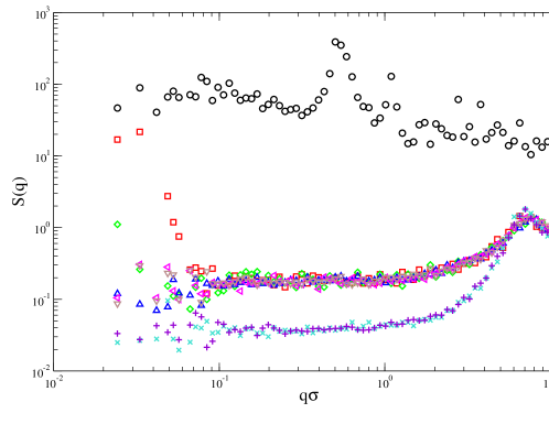
Figure 12: Evolution of structure factor during equilibration process. Structure factor for the annealed lattice (black circle), force-capped KG model after $0.1\tau_{e}$ (red box), $0.5\tau_{e}$ (green diamond), $1\tau_{e}$ (blue triangle up), $5\text{$\tau$}_{e}$ (magenta triangle right), $10\tau_{e}$ (brown triangle down) of simulation, and finally after KG warm for configurations after $5\tau_{e}$ (turquoise cross) or $10\tau_{e}$ (violet plus) of Rouse simulation.

The structure factor during the Rouse simulation and after the KG warm up is shown in Fig. 12. The structure factor measures density fluctuations and when constant allows us to estimate the compressibility of the melt (for derivation see the Appendix). We see that the melt compressibility rapidly decrease by about three orders of magnitude when lattice melt states are equilibrated with the fcKG model. Residual large scale density fluctuations are still observable at $0.1\tau_{e}$, but after $1\tau_{e}$ density fluctuations are absent on all scales. After the KG warm up, the compressibility is further reduced by about one order of magnitude on all scales. This is also seen to be independent of when we perform the KG warm up. A rising tendency of the structure factors are observed at large $q$ values, which is due to the first Bragg peak at $2\pi/\sigma$ and is due to local liquid like bead packing. The structure factors for melts with varying stiffness show similar behavior (data not shown).

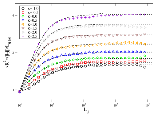
Figure 13: Mean-square internal distances of equilibrated melts (coloured symbols) compared to brute force equilibrated melts (dashed black lines) and Kuhn length (dotted black line) for varying stiffness.

Figure 13 compares the MSID for different stiffness of rapidly equilibrated long melts and brute force equilibrated shorter melts used to estimate the Kuhn lengths. The Rouse simulations were performed for $10\tau_{e}$ when $\kappa<1.5\epsilon$, $20\tau_{e}$ for $\kappa=1.5\epsilon$, $30\tau_{e}$ for $\kappa=2.0\epsilon$, and $40\tau_{e}$ for $\kappa=2.5\epsilon$. Note that since the entanglement time drops rapidly with increasing chain stiffness, the actual run time is largest for the equilibration of the most flexible melts with $\kappa=-1$, which require about a factor of three longer simulation time than the stiffest melts. The chain statistics shown in the figure is in good agreement with the brute force equilibrated melts at short scales, furthermore all the melts levels off to the expected plateau given by the Kuhn length at large scales. A small dip is seen for the two stiffest melts shown in the figure for an intermediate length scale $L_{ij}\approx 100$. Perhaps the stiffest melts are locally nematically ordered, in which case the energy barrier for chain interpenetration could be larger than expected and hence explain why we apparently need to run the simulation for longer than expected from the entanglement time expected from Rouse dynamics. Clearly, the MSID is the measure that is the slowest to converge to the equilibrium since the bulk properties and collective mesoscopic properties measured by the structure factor and melt entanglement length have already reached their equilibrium values after $1\tau_{e}$.

V Conclusions

We have shown how to equilibrate huge model polymer melts in three simple stages for Kremer-Grest polymer melts(Grest and Kremer, 1986) of varying chain stiffness. Firstly, density fluctuations are annealed on scales above the tube scale using simulated annealing with a lattice polymer model. Secondly, with a Molecular Dynamics simulation of a force capped Kremer-Grest (fcKG) polymer model, we simulate the Rouse dynamics(Rouse Jr, 1953) and introduce the desired chain structure on the tube scale and below while preventing the growth of density fluctuations. Finally, we perform a fast warm up to the Kremer-Grest force field to establish the correct local bead packing. We have characterized the involved models in order to transfer melt states between them for varying chain stiffnesses. By measuring the Rouse friction of the fcKG model, we have also estimated the simulation time required for the equilibration of chain structure inside the tube, which was shown to be strongly dependent on chain stiffness.

We have also characterized and validated the equilibration process in terms of 1) single chain observables such as mean-square internal distances, 2) collective mesoscopic melt properties such as the evolution of the entanglement length during the Rouse dynamics, and 3) bulk melt density fluctuations in terms of structure factors. We have demonstrated the convergence of these observables to their equilibrium values for varying chain stiffness.

The main requirement of a equilibration process is computational performance. Here we have equilibrated $15$ melts of $500$ chains with $10.000$ beads each for varying stiffness, and several melts of $1.000$ chains of $15.000$ beads each for varying lattice annealing parameters. For the latter melts, the lattice annealing of density fluctuations takes about $3$ days computer time using a single core on a standard laptop ($72$ core hours). Rouse simulation with the fcKG model for $10\tau_{e}$ takes about 2 days on 4 ABACUS2 nodes(Aba, ), i.e. $4.600$ core hours of compute time. Finally introducing the full KG model, requires about 2 hours on 4 nodes, i.e. $200$ core hours. Moreira(Moreira et al., 2015) equilibrated $1.000\times 2.000$ melts using $3.500$ core hours for pre-packing (equivalent to our lattice annealing), and $3.800$ core hours for subsequent warm up. Zhang et al. (Zhang et al., 2014) equilibrated similar sized melts but using a multiscale method that required $1.600$ core hours. Scaling these numbers to a standard melt of one million beads, the method of Moreira et al. would require $3.600$ core hours, the method of Zhang et al. would requires $800$ core hours, while our method would require $600$ core hours. This could be further optimized e.g. the choice of the force cap is entirely serendipitous, and we use the standard values of the Kremer-Grest polymer model, which could be optimized further.

The present method is essentially independent of e.g. chain length and the polymer structure. These only impacts the lattice annealing stage of the equilibration procedure, which is the fastest part of the equilibration process. The Rouse simulation and KG warm up are completely independent of the chain structure and composition. Hence the present method can directly be used to equilibrate e.g. polymer melts of stars or mixtures of different polymer structures. Furthermore, the equilibrated KG melt configurations produced by the present approach can be fine-grained further to act as starting points for atomistic simulations of polymer melts.

With simple and computationally efficient equilibration approaches such as the one presented here, access to well equilibrated melts for studies of material properties is no longer a computational limitation, rather the limitation is the computational effort required to estimate the material properties of these huge systems.

VI Acknowledgements

Computation/simulation for the work described in this paper was supported by the DeiC National HPC Center at University of Southern Denmark.

VII Appendix

Below we derive predictions for the structure factor due to the density fluctuations created by randomly inserting polymers in the simulation box, and the structure factor after equilibration of density fluctuations and its relation to the compressibility.

Defining the microscopic density as microscopic density field $\rho({\bf R})=\sum_{j=1}^{M}\sum_{k=1}^{N}\delta({\bf R}-{\bf R}_{jk})$, where $\delta$ denotes the Dirac-delta function. We can then recognize the Fourier transform of the density field is $\rho({\bf q})=\sum_{j=1}^{M}\sum_{k=1}^{N_{b}}\exp(i{\bf q}\cdot{\bf R}_{jk})$, such that the structure factor can be written

$$S(q)=\left(N_{b}M\right)^{-1}\langle\rho(-{\bf q})\rho({\bf q})\rangle$$ (12)

To derive the structure factor after equilibration of density fluctuation, we start by expressing the structure factor in terms of spatially varying densities. From the right hand side of eq. 12 we get

$$S({\bf q})=\left\langle\int\mbox{d}{\bf R}_{1}{\bf\mbox{d}}{\bf R}_{2}\rho({\bf R}_{1})\rho({\bf R}_{2})\exp(i{\bf q}\cdot({\bf R}_{1}-{\bf R}_{2}))\right\rangle$$

$$=\int\mbox{d}{\bf R}_{1}{\bf\mbox{d}}{\bf R}_{2}\exp(i{\bf q}\cdot({\bf R}_{1}-{\bf R}_{2}))\left\langle\delta\rho({\bf R}_{1})\delta\rho({\bf R}_{2})\right\rangle$$

$$=\int\mbox{d}{\bf R}\exp(i{\bf q}\cdot{\bf R})\left\langle\delta\rho(0)\delta\rho({\bf R})\right\rangle$$ (13)

where in the second equation we have replaced $\rho({\bf R})\rightarrow\delta\rho({\bf R})=\rho({\bf R})-\langle\rho\rangle$. The constant average density gives rise to a contribution proportional to a Dirac-delta function, which can be neglected for $q>0$. In the third equation, we have furthermore assumed translational invariance.

Lets assume a local Hamiltonian for density fluctuations $H(\delta\rho)=\frac{1}{2\chi\langle\rho\rangle}\delta\rho^{2}$ for a particular position analogous to a site in the lattice model. The Boltzmann probability of a given density fluctuation is given by $P(\delta\rho)\propto\exp(-H/kT)$, and hence $\left\langle\delta\rho^{2}\right\rangle=\chi\langle\rho\rangle kT$ by the equipartition theorem. Assuming that the density fluctuations at different sites are statistically independent, which in practice is valid for sufficiently large distances, i.e. small values of $q$. The density fluctuation correlation function is then given by $\left\langle\delta\rho(0)\delta\rho({\bf R})\right\rangle=\chi\langle\rho\rangle kT\delta({\bf R})$. Inserting this in eq. 13, we obtain the prediction that the structure factor is independent of $q$ and proportional to the compressibility

$$S(q)=\chi\langle\rho\rangle kT.$$

We can also predict the structure factor for polymers randomly inserted into the simulation domain using the approach in Refs. (Svaneborg and Pedersen, 2012a, b). By introducing an origin of the coordinate system for each polymer ${\bf R}_{j}^{o}$ e.g. one of its ends, we can rewrite eq. 6 as

$$S(q)=\left(N_{b}M\right)^{-1}\sum_{k_{1}=1}^{N_{b}}\sum_{k_{2}=1}^{N_{b}}\left[\sum_{j=1}^{M}\left\langle\exp(i{\bf q}\cdot\left({\bf R}_{jk_{1}}-{\bf R}_{jk_{2}}\right))\right\rangle\right.$$

$$\left.+\sum_{\begin{array}[]{c}j_{1},j_{2}=1\\ j_{1}\neq j_{2}\end{array}}^{M}\left\langle\exp(i{\bf q}\cdot\left[\left({\bf R}_{j_{1}k_{1}}-{\bf R}_{j_{1}}^{o}\right)-\left({\bf R}_{j_{2}k_{2}}-{\bf R}_{j_{2}}^{o}\right)+\left({\bf R}_{j_{1}}^{o}-{\bf R}_{j_{2}}^{o}\right)\right])\right\rangle\right],$$

here the first term describes the single polymer scattering due to pairs of scattering sites on the same polymer, while the second term is the interference contribution between scattering sites on different polymers. Configurations of different polymers are generated independently of each other, and the starting points of the polymers are chosen randomly. Hence the three terms in parenthesis in the second exponential are sampled from statistically independent distributions. Having noted this, the average of the interference contribution factorize exactly into a product of three averages, where the first and third only depend on single chain statistics, while the second term only depends on the distance distribution between randomly chosen points:

$$\left\langle\exp(i{\bf q}\cdot\left({\bf R}_{j_{1}k_{1}}-{\bf R}_{j_{1}}^{o}\right))\right\rangle_{j_{1},k}\left\langle\exp(i{\bf q}\cdot\left({\bf R}_{j_{1}}^{o}-{\bf R}_{j_{2}}^{o}\right))\right\rangle_{j_{1},j_{2}}\left\langle\exp(-i{\bf q}\cdot\left({\bf R}_{j_{2}k_{2}}-{\bf R}_{j_{2}}^{o}\right))\right\rangle_{j_{2},k_{2}}.$$

For notational simplicity, we can identify the average form factor as $F({\bf q})=\left\langle\exp(i{\bf q}\cdot\left({\bf R}_{jk_{1}}-{\bf R}_{jk_{2}}\right))\right\rangle_{j,k_{1},k_{2}}$ with the average single polymer scattering, $A({\bf q})=\left\langle\exp(i{\bf q}\cdot\left({\bf R}_{jk_{1}}-{\bf R}_{j}^{o}\right))\right\rangle_{j,k_{1}}$ with the average form factor amplitude relative to an end, and the average phase factor between different ends $\Psi({\bf q})=\left\langle\exp(i{\bf q}\cdot\left[\left({\bf R}_{j_{1}}^{o}-{\bf R}_{j_{2}}^{o}\right)\right])\right\rangle_{j_{1}\neq j_{2}}$. Note all these factors are normalized as $F({\bf q})=A({\bf q})=\Psi({\bf q})\rightarrow 1$ for ${\bf q}\rightarrow 0$. With these simplifications, the structure factor reduce to the much shorter expression

$$S({\bf q})=N_{b}F({\bf q})+(M-1)N_{b}A({\bf q})\Psi({\bf q})A(-{\bf q}).$$

this expression is exact and was derived without any assumptions as to the detailed structure of the objects inserted in the simulation domain and only results from the assumption of statistical independence of intrnal conformations and positions of the objects.(Svaneborg and Pedersen, 2012a) For polymers modeled as ideal random walks, the expressions for the form factor and form factor amplitude are well known(Debye, 1947; Hammouda, 1992):

$$F(q)=\frac{2\left[\exp(-q^{2}R_{g}^{2})-1+q^{2}R_{g}^{2}\right]}{q^{4}R_{g}^{4}}\sim\frac{2}{q^{2}R_{g}^{2}},$$

$$A(q)=\frac{1-\exp(-q^{2}R_{g}^{2})}{q^{2}R_{g}^{2}}\sim\frac{1}{q^{2}R_{g}^{2}},$$

since random walks on average are isotropic, these functions only depends on the magnitude of the scattering vector $q=|{\bf q}|$. The asymptotic behavior is realized for $qR_{g}\gg 1$, where $R_{g}=l_{K}^{2}N_{k}/6$ is the radius of gyration of the polymer. Furthermore, because polymers pairs are placed randomly in the box their starting positions are statistically independent, hence $\Psi({\bf q})=1$. Hence for randomly inserted polymers, the asymptotic behavior of the structure factor describing the resulting density fluctuation correlations is

$$S(q)\sim\frac{2N_{b}}{q^{2}R_{g}^{2}}.$$

References

- Snijkers et al. (2015) F. Snijkers, R. Pasquino, P. Olmsted, and D. Vlassopoulos, J. Phys. Condens. Matter. 27, 473002 (2015).
- Padding and Briels (2011) J. Padding and W. Briels, J. Phys. Condens. Matter 23, 233101 (2011).
- Li et al. (2013) Y. Li, B. C. Abberton, M. Kröger, and W. K. Liu, Polymers 5, 751 (2013).
- Everaers et al. (2004) R. Everaers, S. K. Sukumaran, G. S. Grest, C. Svaneborg, A. Sivasubramanian, and K. Kremer, Science 303, 823 (2004).
- Doi and Edwards (1986) M. Doi and S. F. Edwards, The Theory of Polymer Dynamics (Claredon Press, Oxford, 1986).
- de Gennes (1971) P.-G. de Gennes, J. Chem. Phys. 55, 572 (1971).
- de Gennes (1976) P.-G. de Gennes, Macromolecules 9, 587 (1976).
- Klein (1978) J. Klein, Nature 271, 143 (1978).
- Zamponi et al. (2005) M. Zamponi, M. Monkenbusch, L. Willner, A. Wischnewski, B. Farago, and D. Richter, Europhys. Lett. 72, 1039 (2005).
- Pearson and Helfand (1984) D. S. Pearson and E. Helfand, Macromolecules 17, 888 (1984).
- Brown et al. (1994) D. Brown, J. H. R. Clarke, M. Okuda, and T. Yamazaki, J. Chem. Phys. 100 (1994).
- Auhl et al. (2003) R. Auhl, R. Everaers, G. S. Grest, K. Kremer, and S. J. Plimpton, J. Chem. Phys. 119, 12718 (2003).
- Gao (1995) J. Gao, J. Chem. Phys. 102, 1074 (1995).
- Perez et al. (2008) M. Perez, O. Lame, F. Leonforte, and J.-L. Barrat, J. Chem. Phys. 128, 234904 (2008).
- Karayiannis et al. (2002a) N. C. Karayiannis, V. G. Mavrantzas, and D. N. Theodorou, Phys. Rev. Lett. 88, 105503 (2002a).
- Mavrantzas et al. (1999) V. G. Mavrantzas, T. D. Boone, E. Zervopoulou, and D. N. Theodorou, Macromolecules 32, 5072 (1999).
- Pant and Theodorou (1995) P. K. Pant and D. N. Theodorou, Macromolecules 28, 7224 (1995).
- Karayiannis et al. (2002b) N. C. Karayiannis, A. E. Giannousaki, V. G. Mavrantzas, and D. N. Theodorou, J. Chem. Phys. 117, 5465 (2002b).
- Uhlherr et al. (2002) A. Uhlherr, M. Doxastakis, V. Mavrantzas, D. Theodorou, S. Leak, N. Adam, and P. Nyberg, Europhys. Lett. 57, 506 (2002).
- Karayiannis et al. (2003) N. C. Karayiannis, A. E. Giannousaki, and V. G. Mavrantzas, J. Chem. Phys. 118, 2451 (2003).
- Peristeras et al. (2005) L. D. Peristeras, I. G. Economou, and D. N. Theodorou, Macromolecules 38, 386 (2005).
- Ramos et al. (2007) J. Ramos, L. D. Peristeras, and D. N. Theodorou, Macromolecules 40, 9640 (2007).
- Daoulas et al. (2002) K. C. Daoulas, A. F. Terzis, and V. G. Mavrantzas, J. Chem. Phys. 116, 11028 (2002).
- Daoulas et al. (2003) K. C. Daoulas, A. F. Terzis, and V. G. Mavrantzas, Macromolecules 36, 6674 (2003).
- Subramanian (2010) G. Subramanian, J. Chem. Phys. 133, 164902 (2010).
- Subramanian (2011) G. Subramanian, Macromol. Theory Simul. 20, 46 (2011).
- Zhang et al. (2014) G. Zhang, L. A. Moreira, T. Stuehn, K. C. Daoulas, and K. Kremer, ACS Macro. Lett. 3, 198 (2014).
- Moreira et al. (2015) L. A. Moreira, G. Zhang, F. Müller, T. Stuehn, and K. Kremer, Macromol. Theory Simul. 24, 419 (2015).
- Theodorou and Suter (1985) D. N. Theodorou and U. W. Suter, Macromolecules 18, 1467 (1985).
- Theodorou and Suter (1986) D. N. Theodorou and U. W. Suter, Macromolecules 19, 139 (1986).
- Carbone et al. (2010) P. Carbone, H. A. Karimi-Varzaneh, and F. Müller-Plathe, Faraday Discuss. 144, 25 (2010).
- Kotelyanskii et al. (1996) M. Kotelyanskii, N. Wagner, and M. E. Paulaitis, Macromolecules 29, 8497 (1996).
- Sliozberg et al. (2016) Y. R. Sliozberg, M. Kröger, and T. L. Chantawansri, The Journal of Chemical Physics 144, 154901 (2016).
- Grest and Kremer (1986) G. S. Grest and K. Kremer, Phys. Rev. A 33, 3628 (1986).
- Svaneborg et al. (2016) C. Svaneborg, H. Karimi-Varzaneh, N. Hojdis, and R. Everaers, “Kremer-Grest models of common polymer melts. Manuscript submitted.” (2016).
- Hoogerbrugge and Koelman (1992) P. Hoogerbrugge and J. Koelman, Europhys. Lett. 19, 155 (1992).
- Espanol and Warren (1995) P. Espanol and P. Warren, Europhys. Lett. 30, 191 (1995).
- Flory (1949) P. J. Flory, J. Chem. Phys. 17, 303 (1949).
- Flory and Jackson (1989) P. Flory and J. Jackson, Statistical Mechanics of Chain Molecules (Hanser, 1989).
- Edwards (1967) S. Edwards, 91, 513 (1967).
- Rouse Jr (1953) P. E. Rouse Jr, J. Chem. Phys. 21, 1272 (1953).
- Everaers (2012) R. Everaers, Phys. Rev. E. 86, 022801 (2012).
- Kremer and Grest (1990) K. Kremer and G. S. Grest, J. Chem. Phys. 92, 5057 (1990).
- Faller et al. (1999) R. Faller, A. Kolb, and F. Müller-Plathe, Phys. Chem. Chem. Phys. 1, 2071 (1999).
- Faller et al. (2000) R. Faller, F. Müller-Plathe, and A. Heuer, Macromolecules 33, 6602 (2000).
- Faller and Müller-Plathe (2001) R. Faller and F. Müller-Plathe, Chem. Phys. Chem. 2, 180 (2001).
- Grønbech-Jensen and Farago (2013) N. Grønbech-Jensen and O. Farago, Mol. Phys. 111, 983 (2013).
- Grønbech-Jensen et al. (2014) N. Grønbech-Jensen, N. R. Hayre, and O. Farago, Comp. Phys. Comm. 185, 524 (2014).
- Plimpton (1995) S. Plimpton, J. Comp. Phys. 117, 1 (1995).
- Sukumaran et al. (2005) S. K. Sukumaran, G. S. Grest, K. Kremer, and R. Everaers, J. Polym. Sci., Part B: Polym. Phys. 43, 917 (2005).
- Fetters et al. (2007) L. Fetters, D. Lohse, and R. Colby, in Physical properties of polymers handbook, edited by J. Mark (Springer, 2007) pp. 447–454.
- Wang (2009) Q. Wang, Soft Matter 5, 4564 (2009).
- Helfand and Tagami (1971) E. Helfand and Y. Tagami, J. Polym. Sci. B. 9, 741 (1971).
- Helfand and Tagami (1972) E. Helfand and Y. Tagami, J. Chem. Phys. 56, 3592 (1972).
- Madras and Sokal (1988) N. Madras and A. D. Sokal, J. Stat. Phys. 50, 109 (1988).
- Wittmer et al. (2007a) J. Wittmer, P. Beckrich, A. Johner, A. Semenov, S. Obukhov, H. Meyer, and J. Baschnagel, Europhys. Lett. 77, 56003 (2007a).
- Wittmer et al. (2007b) J. Wittmer, P. Beckrich, H. Meyer, A. Cavallo, A. Johner, and J. Baschnagel, Phys. Rev. E. 76, 011803 (2007b).
- Beckrich et al. (2007) P. Beckrich, A. Johner, A. N. Semenov, S. P. Obukhov, H. Benoit, and J. Wittmer, Macromolecules 40, 3805 (2007).
- Meyer et al. (2008) H. Meyer, J. Wittmer, T. Kreer, P. Beckrich, A. Johner, J. Farago, and J. Baschnagel, Eur. Phys. J. E. 26, 25 (2008).
- Semenov (2010) A. Semenov, Macromolecules 43, 9139 (2010).
- Sides et al. (2004) S. W. Sides, G. S. Grest, M. J. Stevens, and S. J. Plimpton, J. Polym. Sci., Part B: Polym. Phys. 42, 199 (2004).
- Hoy et al. (2009) R. S. Hoy, K. Foteinopoulou, and M. Kröger, Phys. Rev. E 80, 031803 (2009).
- Zhang et al. (2015) G. Zhang, T. Stuehn, K. C. Daoulas, and K. Kremer, J. Chem. Phys. 142, 221102 (2015).
- Hoy and Robbins (2005) R. S. Hoy and M. O. Robbins, Physical Review E 72, 61802 (2005).
- (65) “Hardware setup of the abacus 2.0 cluster at the university of southern denmark. https://deic.sdu.dk/setup/hardware,” .
- Svaneborg and Pedersen (2012a) C. Svaneborg and J. S. Pedersen, J. Chem. Phys. 136, 104105 (2012a).
- Svaneborg and Pedersen (2012b) C. Svaneborg and J. S. Pedersen, J. Chem. Phys. 136, 154907 (2012b).
- Debye (1947) P. Debye, J. Phys. Colloid Chem. 51, 18 (1947).
- Hammouda (1992) B. Hammouda, J. Polym. Sci., Part B: Polym. Phys. 30, 1387 (1992).