All-coupling polaron optical response: analytic approaches beyond the adiabatic approximation

Abstract

In the present work, the problem of an all-coupling analytic description for the optical conductivity of the Fröhlich polaron is treated, with the goal being to bridge the gap in validity range that exists between two complementary methods: on the one hand the memory function formalism and on the other hand the strong-coupling expansion based on the Franck-Condon picture for the polaron response. At intermediate coupling, both methods were found to fail as they do not reproduce Diagrammatic Quantum Monte Carlo results. To resolve this, we modify the memory function formalism with respect to the Feynman-Hellwarth-Iddings-Platzman (FHIP) approach, in order to take into account a non-quadratic interaction in a model system for the polaron. The strong-coupling expansion is extended beyond the adiabatic approximation, by including into the treatment non-adiabatic transitions between excited polaron states. The polaron optical conductivity that we obtain by combining the two extended methods agree well, both qualitatively and quantitatively, with the Diagrammatic Quantum Monte Carlo results in the whole available range of the electron-phonon coupling strength.

I Introduction

The polaron, first proposed as a physical concept by L. D. Landau Landau in the context of electrons in polar crystals, has become a generic notion describing a particle interacting with a quantized bosonic field. The polaron problem has consequently been used for a long time as a testing ground for various analytic and numerical methods with applications in quantum statistical physics and quantum field theory. In condensed matter physics, the polaron effect coming from the electron-phonon interaction is a necessary ingredient in the description of the DC mobility and the optical response in polar crystals (see Ref. Devreese2009 ). Polaronic effects are manifest in many interesting systems, such as magnetic polarons Hemolt , polarons in semiconducting polymers Sirringhaus , and complex oxides Franchini1 ; Franchini2015 which are described in terms of the small-polaron theory Holstein . Large-polaron theory has recently been stimulated by the possibility to study polaronic effects using highly tunable quantum gases: the physics of an impurity immersed in an atomic Bose-Einstein condensateBECpol2 can be modeled on the basis of a Fröhlich Hamiltonian. Another recent development in large-polaron physics stems from the experimental advances in the determination of the band structure of highly polar oxides Meevasana , relevant for superconductivity, where the optical response of complex oxides explicitly shows the large-polaron features Mechelen2008 ; PRB2010 .

Diagrammatic Quantum Monte Carlo (DQMC) methods have been applied in recent years to numerically calculate the ground state energy and the optical conductivity of the Fröhlich polaron M2000 ; M2003 . Advances in computational techniques such as DQMC inspired renewed study of the key problem in polaron theory – an analytic description of the polaron response. For the small-polaron optical conductivity, the all-coupling analytic theory has been successfully developed Berciu showing good agreement with the numeric results of the DQMC. However, the optical response problem for a large polaron is not yet completely solved analytically.

Asymptotically exact analytic solutions for the polaron optical conductivity have been obtained in the limits of weak GLF ; DHL1971 and strong coupling PRL2006 ; PRB2014 . A first proposal for an all-coupling approximation for the polaron optical conductivity has been formulated in Ref. DSG (below referred to as DSG), further developing the Feynman-Hellwarth-Iddings-Platzman theory FHIP (FHIP) and using the Feynman variational approach Feynman . However, in Ref. DSG , it was already demonstrated that FHIP at large $\alpha$ is inconsistent with the Heisenberg uncertainty relations. This inconsistency is revealed in Ref. DSG through extremely narrow peaks of the optical conductivity at large $\alpha$. Nevertheless, the peak positions for the polaron optical conductivity as obtained in Ref. DSG have been confirmed with high accuracy PRB2014 by the DQMC calculation M2003 . This inspired further attempts to develop analytical methods for the polaron optical response, especially at intermediate and strong coupling. Among these analytic methods, an extension of the DSG method has been proposed in Ref. PRL2006 introducing an extended memory function formalism with a relaxation time determined from the additional sum rule for the polaron optical conductivity. Alternatively, for the strong coupling regime, the strong coupling expansion (SCE) based on the Franck-Condon scheme for multiphonon optical conductivity has been developed in Refs. PRL2006 ; PRB2014 .

The extended memory-function formalism and the strong coupling expansion of Ref. PRL2006 are complementary to each other. The memory-function formalism is well-substantiated for small and intermediate values of $\alpha$, and the strong coupling expansion adequately describes the opposite limit of large $\alpha$. However these two methods only qualitatively agree with each other and with the DQMC data in the range of intermediate coupling strengths. On one hand, the memory function formalism disagrees with DQMC at large $\alpha$. On the other hand, the strong-coupling expansion only qualitatively reproduces the shape of the optical conductivity and fails at intermediate $\alpha$. The main aim of the current paper is to extend both the memory function formalism and the strong coupling expansion in order to bridge the gap that remains between their regions of validity, such that the combination of both methods allows to find analytical results in agreement with the numeric DQMC results at all coupling.

We have added the following new elements in the theory which lead to an overlapping of the areas of applicability for two aforesaid analytic methods. For weak and intermediate coupling strengths, an extension of the Feynman variational principle and the memory-function method for a polaron with a non-quadratic trial action has been developed. As distinct from the memory function formalism of Ref. PRL2006 , we do not use additional sum rules and relaxation times, and perform the calculation ab initio. For intermediate and strong coupling strengths, the strong coupling expansion of Ref. PRB2014 is extended beyond the adiabatic approximation accounting for non-adiabatic transitions between excited polaron states. This leads to a substantial expansion of the range of validity for the strong-coupling expansion towards smaller $\alpha$ and to an overall improvement of its agreement with DQMC.

The paper is organized as follows. In Sec. II we describe an all-coupling analytic description for the polaron optical conductivity within the extended memory function formalism with a non-parabolic trial action and the non-adiabatic strong-coupling expansion. Sec. III contains the discussion of the obtained optical conductivity spectra and their comparison with results of other methods and with the DQMC data. The discussion is followed by conclusions, Sec. IV.

II Analytic methods for the polaron optical conductivity

II.1 Memory function formalism with a non-parabolic trial action

To generalize the memory function formalism, we start by extending Feynman’s variational approach to translation invariant non-Gaussian trial actions. The electron-phonon system is described by the Fröhlich Hamiltonian, using the Feynman units with $\hbar=1,$ the LO-phonon frequency $\omega_{\mathrm{LO}}=1$, and the band mass $m_{b}=1$,

$$\hat{H} =\frac{\mathbf{\hat{p}}^{2}}{2}+\sum_{\mathbf{q}}\left(\hat{a}_{\mathbf{q}}^{+}\hat{a}_{\mathbf{q}}+\frac{1}{2}\right)$$

$$+\frac{1}{\sqrt{V}}\sum_{\mathbf{q}}\frac{\sqrt{2\sqrt{2}\pi\alpha}}{q}\left(\hat{a}_{\mathbf{q}}+\hat{a}_{-\mathbf{q}}^{+}\right)e^{i\mathbf{q\cdot\hat{r}}},$$ (1)

where $\mathbf{\hat{r}}$ is the position operator of the electron, $\mathbf{\hat{p}}$ is its momentum operator; $\hat{a}_{\mathbf{q}}^{\dagger}$ and $\hat{a}_{\mathbf{q}}$ are, respectively, the creation and annihilation operators for longitudinal optical (LO) phonons of wave vector $\mathbf{q}$. The electron-phonon coupling strength is described by the Fröhlich coupling constant $\alpha$. As this Hamiltonian is quadratic in the phonon degrees of freedom, they can be integrated out analytically in the path-integral approach Feynman . The remaining electron degree of freedom is described via an action functional where the effects of electron-phonon interaction are contained in an influence phase:

$$S[\mathbf{r}_{e}(\tau)]=\frac{1}{2}{\displaystyle\int\limits_{0}^{\beta}}\mathbf{\dot{r}}_{e}^{2}(\tau)d\tau-\Phi[\mathbf{r}_{e}(\tau)].$$ (2)

Here $\mathbf{r}_{e}(\tau)$ is the path of the electron, expressed in imaginary time so as to obtain the euclidean action, and $\beta=1/(k_{B}T)$ with $T$ the temperature. The influence phase corresponding to (1) is

$$\Phi[\mathbf{r}_{e}(\tau)] =\sqrt{2}\pi\alpha\int\frac{d\mathbf{q}}{(2\pi)^{3}}{\displaystyle\int\limits_{0}^{\beta}}d\tau{\displaystyle\int\limits_{0}^{\beta}}d\tau^{\prime}\frac{\cosh\left(\left|\tau-\tau^{\prime}\right|-\frac{\beta}{2}\right)}{\sinh(\beta/2)}$$

$$\times e^{i\mathbf{q}\cdot\left[\mathbf{r}_{e}(\tau)-\mathbf{r}_{e}(\tau^{\prime})\right]}.$$ (3)

This depends on the difference in electron position at different times, resulting in a retarded action functional. In the path-integral formalism, thermodynamic potentials (such as the free energy) are calculated via the partition sum, which in turn is written as a sum over all possible paths $\mathbf{r}_{e}(\tau)$ of the electron that start and end in the same point, weighted by the exponent of the action:

$$e^{-\beta F}=\mathcal{Z}=\int\mathcal{D}\mathbf{r}_{e}e^{-S[\mathbf{r}_{e}(\tau)]}.$$ (4)

Feynman’s original variational method considers a quadratic trial action where the phonon degrees of freedom are replaced a fictitious particle with coordinate $\mathbf{r}_{f}(\tau)$,

$$S_{\text{quad}}\left[\mathbf{r}_{e}(\tau),\mathbf{r}_{f}(\tau)\right] ={\displaystyle\int\limits_{0}^{\beta}}\left[\frac{m\mathbf{\dot{r}}_{e}^{2}}{2}\right.$$

$$\left.+\frac{m_{f}\mathbf{\dot{r}}_{f}^{2}}{2}+V\left(\mathbf{r}_{f}-\mathbf{r}_{e}\right)\right]d\tau,$$ (5)

interacting with the electron through a harmonic potential:

$$V\left(\mathbf{r}_{f}-\mathbf{r}_{e}\right)=\frac{m_{f}\omega^{2}}{2}\left(\mathbf{r}_{f}-\mathbf{r}_{e}\right)^{2}.$$ (6)

The partition sum corresponding to this model is

$$\mathcal{Z}_{\text{quad}}=\int\mathcal{D}\mathbf{r}_{e}\int\mathcal{D}\mathbf{r}_{f}e^{-S_{\text{quad}}[\mathbf{r}_{e}(\tau),\mathbf{r}_{f}(\tau)]}.$$ (7)

Expectation values of of functionals $\mathcal{F}[\mathbf{r}_{e}(\tau)]$ of the electron path are given by

$$\left\langle\mathcal{F}[\mathbf{r}_{e}(\tau)]\right\rangle_{\text{quad}} =\frac{1}{\mathcal{Z}_{\text{quad}}}\int\mathcal{D}\mathbf{r}_{e}\text{ }\mathcal{F}[\mathbf{r}_{e}(\tau)]$$

$$\times\int\mathcal{D}\mathbf{r}_{f}e^{-S_{\text{quad}}[\mathbf{r}_{e}(\tau),\mathbf{r}_{f}(\tau)]}.$$ (8)

In the above formula, it is clear that performing the path integral over $\mathbf{r}_{f}$ exactly may simplify the result. The result of this integration still depends on the path $\mathbf{r}_{e}(\tau)$ and is written in terms of an influence phase,

$$\int\mathcal{D}\mathbf{r}_{f}\exp\left\{-{\displaystyle\int\limits_{0}^{\beta}}\left[\frac{m_{f}\mathbf{\dot{r}}_{f}^{2}}{2}+\frac{m_{f}\omega^{2}}{2}\left(\mathbf{r}_{f}-\mathbf{r}_{e}\right)^{2}\right]d\tau\right\}$$

$$=\mathcal{Z}_{f}\exp\left\{\Phi_{\text{quad}}[\mathbf{r}_{e}(\tau)]\right\},$$ (9)

where $\mathcal{Z}_{f}$ is a constant independent of $\mathbf{r}_{e}(\tau)$. The influence phase corresponds to a quadratic, retarded interaction for the electron. The model system partition sum becomes

$$\mathcal{Z}_{\text{quad}}=\mathcal{Z}_{f}\int\mathcal{D}\mathbf{r}_{e}\exp\left\{-{\displaystyle\int\limits_{0}^{\beta}}\frac{m\mathbf{\dot{r}}_{e}^{2}}{2}d\tau+\Phi_{\text{quad}}[\mathbf{r}_{e}(\tau)]\right\}.$$ (10)

Feynman restricted his trial action to a quadratic action, since only for case one can calculate the influence phase analytically, and obtain

$$\Phi_{\text{quad}}[\mathbf{r}_{e}(\tau)] =-\frac{m_{f}\omega^{3}}{4}{\displaystyle\int\limits_{0}^{\beta}}d\tau{\displaystyle\int\limits_{0}^{\beta}}d\tau^{\prime}\left[\mathbf{r}_{e}(\tau)-\mathbf{r}_{e}(\tau^{\prime})\right]^{2}$$

$$\times\frac{\cosh\left[\omega\left(\left|\tau-\tau^{\prime}\right|-\frac{\beta}{2}\right)\right]}{\sinh(\beta\omega/2)}.$$ (11)

The essence of the Feynman variational method consists in writing the partition function of the true electron-phonon system (2) as

$$\mathcal{Z} =\frac{1}{\mathcal{Z}_{f}}\int\mathcal{D}\mathbf{r}_{e}\exp\left\{\Phi[\mathbf{r}_{e}(\tau)]-\Phi_{\text{quad}}[\mathbf{r}_{e}(\tau)]\right\}$$

$$\times\int\mathcal{D}\mathbf{r}_{f}\exp\left\{-S_{\text{quad}}[\mathbf{r}_{e}(\tau),\mathbf{r}_{f}(\tau)]\right\}.$$ (12)

Indeed, performing the path integration for the fictitious particle via (9) cancels $\Phi_{\text{quad}}[\mathbf{r}_{e}(\tau)]$ as well as the factor $\mathcal{Z}_{f}$, and leaves the kinetic energy contribution, restoring the action function of the true system. The usefulness of the above expression lies in the fact that it can also be interpreted as an expectation value with respect to the model system:

$$\mathcal{Z}=\frac{\mathcal{Z}_{\text{quad}}}{\mathcal{Z}_{f}}\left\langle\exp\left\{\Phi[\mathbf{r}_{e}(\tau)]-\Phi_{\text{quad}}[\mathbf{r}_{e}(\tau)]\right\}\right\rangle_{\text{quad}}.$$ (13)

Now using Jensen’s inequality

$$\left\langle e^{\mathcal{F}[\mathbf{r}_{e}(\tau)]}\right\rangle\geqslant e^{\left\langle\mathcal{F}[\mathbf{r}_{e}(\tau)]\right\rangle},$$ (14)

and taking the logarithm of the resulting expression leads to

$$F\leqslant F_{0}+\frac{1}{\beta}\left\langle\Phi_{\text{quad}}[\mathbf{r}_{e}(\tau)]-\Phi[\mathbf{r}_{e}(\tau)]\right\rangle_{\text{quad}},$$ (15)

which is the Jensen-Feynman variational inequality. Here we introduce the notation $\mathcal{Z}_{\text{quad}}/\mathcal{Z}_{f}=e^{-\beta F_{0}}$. Note that when we write the above expression in terms of the actions rather than the influence phases, one gets the more familiar form of the Jensen-Feynman inequality:

$$F\leqslant F_{0}+\frac{1}{\beta}\left\langle S[\mathbf{r}_{e}(\tau)]-S_{\text{quad}}[\mathbf{r}_{e}(\tau)]\right\rangle_{\text{quad}}.$$ (16)

Using the Feynman variational approach with the Gaussian trial action, excellent results are obtained for the polaron ground-state energy, free energy, and the effective mass. Moreover, this approach has been effectively used to derive the DSG all-coupling theory for the polaron optical conductivity, Ref. DSG . However, as mentioned in the introduction, the DSG and DQMC results contradict to each other in the range of large $\alpha$. The most probable source of this contradiction is the Gaussian form of the trial action used in the DSG theory. Indeed, the model system contains only a single frequency, leading to unphysically sharp peaks in the spectrum, subject to thermal broadening only Dries1 ; Dries2 . Extensions to the formalism PRL2006 have tried to overcome this problem by including an ad-hoc broadening of the energy level, chosen in such as way as to comply with the sum rules. A remarkable success in the problem of the polaron optical response has been achieved in the recent work DS , where the all-coupling polaron optical conductivity is calculated using the general quadratic trial action instead of the Feynman model with a single fictitious particle. The resulting optical conductivity is in good agreement with DQMC results M2003 in the weak- and intermediate-coupling regimes and is qualitatively in line with DQMC even at extremely strong coupling, resolving the issue of the linewidth in the FHIP approach.

In the literature, there are attempts to re-formulate the Feynman variational approach avoiding retarded trial actions. For example, Cataudella et al. Catau introduce an extended action which contains the coordinates of the electron, the fictitious particle, and the phonons. This action, however, is not exactly equivalent to the action of the electron-phonon system, and hence the results obtained in Catau need verification. In Ref. SSC , we introduced an extended action/Hamiltonian for an electron-phonon system and reformulated the Feynman variational method in the Hamiltonian representation. This method leads to the same result as the Feynman variational approach. However the method of Ref. SSC reproduces the strong coupling limit for the polaron energy only when using a Gaussian trial action.

In the current work, we propose to extend the Feynman variational approach to trial systems with non-parabolic interactions between an electron and a fictitious particle. The difficulty with using non-Gaussian trial actions is that the influence phase (here $\Phi_{\text{quad}}$) can only be computed analytically for quadratic action functionals. However, quantum-statistical expectation values (such as the one in the Jensen-Feynman inequality) can be calculated for non-quadratic model systems by other means, in particular if the spectrum of eigenvalues and eigenfunctions can be found. So, what we propose is to focus on keeping the influence phase for a quadratic model system in the expressions, while at the same time allowing for non-Gaussian potentials for the expectation values.

Consider a (non-quadratic) variational trial action

$$S_{\text{var}}\left[\mathbf{r}_{e}(\tau),\mathbf{r}_{f}(\tau)\right] ={\displaystyle\int\limits_{0}^{\beta}}\left[\frac{m\mathbf{\dot{r}}_{e}^{2}}{2}\right.$$

$$\left.+\frac{m_{f}\mathbf{\dot{r}}_{f}^{2}}{2}+U\left(\mathbf{r}_{f}-\mathbf{r}_{e}\right)\right]d\tau$$ (17)

with a general potential $U$. Since

$$S_{\text{quad}}\left[\mathbf{r}_{e}(\tau),\mathbf{r}_{f}(\tau)\right] =S_{\text{var}}\left[\mathbf{r}_{e}(\tau),\mathbf{r}_{f}(\tau)\right]$$

$$+{\displaystyle\int\limits_{0}^{\beta}}\left[V\left(\mathbf{r}_{f}-\mathbf{r}_{e}\right)-U\left(\mathbf{r}_{f}-\mathbf{r}_{e}\right)\right]d\tau,$$ (18)

we can rewrite (12) to:

$$\mathcal{Z} =\frac{1}{\mathcal{Z}_{f}}\int\mathcal{D}\mathbf{r}_{e}\int\mathcal{D}\mathbf{r}_{f}\exp\left\{\Phi[\mathbf{r}_{e}(\tau)]-\Phi_{\text{quad}}[\mathbf{r}_{e}(\tau)]\right\}$$

$$\times\exp\left\{-{\displaystyle\int\limits_{0}^{\beta}}\left[V\left(\mathbf{r}_{f}-\mathbf{r}_{e}\right)-U\left(\mathbf{r}_{f}-\mathbf{r}_{e}\right)\right]d\tau\right\}$$

$$\times\exp\left\{-S_{\text{var}}\left[\mathbf{r}_{e}(\tau),\mathbf{r}_{f}(\tau)\right]\right\}.$$ (19)

Expectation values of functionals of $\mathbf{r}_{e}(\tau)$ and $\mathbf{r}_{f}(\tau)$ with respect to the non-quadratic variational model system are given by

$$\left\langle\mathcal{F}[\mathbf{r}_{e},\mathbf{r}_{f}]\right\rangle_{\text{var}} =\frac{1}{\mathcal{Z}_{\text{var}}}\int\mathcal{D}\mathbf{r}_{e}\int\mathcal{D}\mathbf{r}_{f}\mathcal{F}[\mathbf{r}_{e},\mathbf{r}_{f}]$$

$$\times\exp\left\{-S_{\text{var}}\left[\mathbf{r}_{e}(\tau),\mathbf{r}_{f}(\tau)\right]\right\}.$$ (20)

This allows to interpret expression (19) as

$$\mathcal{Z} =\frac{\mathcal{Z}_{\text{var}}}{\mathcal{Z}_{f}}\left\langle\exp\left\{\Phi[\mathbf{r}_{e}(\tau)]-\Phi_{\text{quad}}[\mathbf{r}_{e}(\tau)]\right.\right.$$

$$\left.\left.-{\textstyle\int\nolimits_{0}^{\beta}}\left[V\left(\mathbf{r}_{f}-\mathbf{r}_{e}\right)-U\left(\mathbf{r}_{f}-\mathbf{r}_{e}\right)\right]d\tau\right\}\right\rangle_{\text{var}}$$ (21)

With $\mathcal{Z}_{\text{var}}/\mathcal{Z}_{f}=e^{-\beta F_{\text{var}}}$ and using again Jensen’s inequality, we arrive at:

$$F \leqslant F_{\text{var}}+\frac{1}{\beta}\left\langle\Phi_{\text{quad}}[\mathbf{r}_{e}(\tau)]-\Phi[\mathbf{r}_{e}(\tau)]\right\rangle_{\text{var}}$$

$$+\left\langle V\left(\mathbf{r}_{f}-\mathbf{r}_{e}\right)-U\left(\mathbf{r}_{f}-\mathbf{r}_{e}\right)\right\rangle_{\text{var}}$$ (22)

We have used that for time-independent potentials, $\frac{1}{\beta}{\textstyle\int\nolimits_{0}^{\beta}}d\tau=1$. When $U=V$, and we choose a quadratic interaction potential, this restores the original Jensen-Feynman variational principle. However, deviations from a quadratic potential result in two changes. Firstly, there is an additional term corresponding to the expectation value of the difference between the chosen variational potential and the quadratic one. Secondly, the expectation values are to be calculated with respect to the chosen variational potential $U$ rather than with respect to the quadratic potential. We again emphasize that the calculation of such expectation values does not require a quadratic potential.  Thus the new variational inequality (22) is an extension of the Feynman – Jensen inequality.

It is important for the calculations that $S_{\text{var}}$ is translation invariant but non-retarded action, so that all expressions in the variational functional (22) have the same form in both representations – path integral and standard quantum mechanics. Apart from the parameters appearing in the trial action $S_{\text{var}}$, the inequality (22) still contains as variational parameters $m_{f}$ and $\omega$, inherited from the “auxiliary” quadratic action $S_{\text{quad}}$ and appearing in $\Phi_{\text{quad}}$ and $V\left(\mathbf{r}_{f}-\mathbf{r}_{e}\right)$. These do not depend on the parameters of the electron-phonon interaction at all, and therefore the minimization of the free energy with respect to $m_{f}$ and $\omega$ can be performed before the minimization of the whole variational functional with respect to the remaining parameters of the non-Gaussian trial action $S_{\text{var}}$.

The extended Jensen-Feynman inequality (22), despite having more variational parameters, does not lead in general to a substantially lower polaron free energy than the original Feynman result, except in the extremely strong coupling regime, where the present variational functional analytically tends (for $T=0$) to the exact strong coupling limit obtained by Miyake M75 . However, its advantage with respect to the original Feynman treatment is in calculating the optical conductivity. A physically reasonable choice of the trial interaction potential $U\left(\mathbf{r}_{f}-\mathbf{r}\right)$ is no longer restricting to a single frequency oscillator. According to Refs. M75 ; Pekar1954 , the self-consistent potential for an electron induced by the lattice polarization is parabolic near the bottom and Coulomb-like at large distances. Therefore, for the calculation of the optical conductivity, we choose a trial potential in the piecewise form, stitching together a parabolic and a Coulomb-like potential in a continuous way. The spectrum of internal states of the model system with this potential necessarily consists of an infinite number non-equidistant energy levels with the energies $E_{n}<0$ (counted from the potential energy at the infinity distance from the polaron) and a continuum of energies $E>0$. Accounting for transitions between all these levels, one must expect a significant broadening of the peak absorption.

The polaron optical conductivity is calculated using the memory-function formalism which differs from that applied in Refs. DSG ; PD1983 ; PRL2006 by using the non-quadratic trial action described above. The optical conductivity of a gas of interacting polarons within the memory-function technique, is given by the formula which is structurally similar to the polaron optical conductivity DSG ,

$$\sigma\left(\Omega\right)=\frac{e^{2}n_{0}}{m_{b}}\frac{i}{\Omega-\chi\left(\Omega\right)/\Omega},$$ (23)

where $n_{0}=N/V$ is the carrier density. The memory function in the non-quadratic setting is given by

$$\chi\left(\Omega\right) =\frac{2}{3\hbar m_{b}}\int\frac{d\mathbf{q}}{\left(2\pi\right)^{3}}q^{2}\left|V_{\mathbf{q}}\right|^{2}\int_{0}^{\infty}dt\left(e^{i\Omega t}-1\right)$$

$$\times\operatorname{Im}\left[\frac{\cos\left[\omega_{0}\left(t+\frac{i\hbar\beta}{2}\right)\right]}{\sinh\left(\frac{\beta\hbar\omega_{0}}{2}\right)}\left\langle e^{i\mathbf{q\cdot r}\left(t\right)}e^{-i\mathbf{q\cdot r}}\right\rangle_{\text{var}}\right],$$ (24)

where $\omega_{0}$ is the LO phonon frequency, and the correlation function $\left\langle e^{i\mathbf{q\cdot r}\left(t\right)}e^{-i\mathbf{q\cdot r}}\right\rangle_{\text{var}}$ is calculated with the quantum states of the trial Hamiltonian corresponding to $S_{\text{var}}$. In the particular case $T=0$ we apply the formula following from (24)

$$\chi\left(\Omega\right) =\frac{1}{3\pi^{2}\hbar m_{b}}\lim_{\delta\rightarrow 0_{+}}\int_{0}^{\infty}dq~{}\left|V_{\mathbf{q}}\right|^{2}q^{4}\int\limits_{0}^{\infty}dt~{}e^{-\delta t}$$

$$\times\left(e^{i\Omega t}-1\right)\operatorname{Im}\left(e^{-i\omega_{0}t}\left\langle e^{i\mathbf{q\cdot r}\left(t\right)}e^{-i\mathbf{q\cdot r}}\right\rangle_{\text{var}}\right).$$ (25)

Rather than computing the correlation function $\left\langle e^{i\mathbf{q\cdot r}\left(t\right)}e^{-i\mathbf{q\cdot r}}\right\rangle_{\text{var}}$ as a path integral through (20), we choose to evaluate it in the equivalent Hamiltonian formalism. In this Hamiltonian framework, (25) is written as a sum over the eigenstates of the trial Hamiltonian for the electron and the fictitious particle interacting through the potential $U$,

$$\hat{H}_{\text{var}}=\frac{\mathbf{\hat{p}}^{2}}{2}+\frac{\mathbf{\hat{p}}_{f}^{2}}{2m_{f}}+U\left(\mathbf{\hat{r}}_{f}-\mathbf{\hat{r}}\right).$$ (26)

Thus the correlation function is given by:

$$\left\langle e^{i\mathbf{q\cdot r}\left(t\right)}e^{-i\mathbf{q\cdot r}}\right\rangle_{\text{var}} =\sum_{\mathbf{k}^{\prime};l^{\prime},n^{\prime},m^{\prime}}e^{i\frac{t}{\hbar}\left[\left(\varepsilon_{0,0}-\varepsilon_{l^{\prime},n^{\prime}}\right)-\frac{\hbar^{2}\left(\mathbf{k}^{\prime}\right)^{2}}{2M}\right]}$$

$$\times\left|\left\langle\psi_{\mathbf{0};0,0,0}\left|e^{i\mathbf{q\cdot r}}\right|\psi_{\mathbf{k}^{\prime};l^{\prime},n^{\prime},m^{\prime}}\right\rangle\right|^{2},$$ (27)

where $M=1+m_{f}$ is the total mass of the trial system and $\left|\psi_{\mathbf{k};l,n,m}\right\rangle$ are the wave functions of the trial system. The wave function $\left|\psi_{\mathbf{k};l,n,m}\right\rangle$ is factorized as a product of a plane wave for the center-of-mass motion (with center-of-mass coordinate $\mathbf{R}$) and a wave function for the relative motion $\left|\varphi_{l,n,m}\right\rangle$ (with the coordinate vector $\boldsymbol{\rho}$ of the relative motion),

$$\left|\psi_{\mathbf{k};l,n,m}\right\rangle =\frac{1}{\sqrt{V}}e^{i\mathbf{k\cdot R}}\left|\varphi_{l,n,m}\right\rangle,$$ (28)

$$\left|\varphi_{l,n,m}\right\rangle =\mathcal{R}_{l,n}\left(\rho\right)Y_{l,m}\left(\theta,\varphi\right).$$ (29)

The quantum numbers for the Hamiltonian $\hat{H}_{\text{var}}$ are the momentum $\mathbf{k}$, the quanta $l,m$ related to to angular momentum, and a nodal quantum number $n$ for the relative motion wavefunction. The quantum numbers $l,n$ determine the energy $\varepsilon_{l,n}$ associated with the relative motion between electron and fictitious particle (including both the discrete and continuous parts of the energy spectrum). When substituting (27) into the memory function we arrive at the result

$$\chi\left(\Omega\right) =\frac{1}{3\pi^{2}\hbar m_{b}}\int_{0}^{\infty}dq~{}\left|V_{\mathbf{q}}\right|^{2}q^{4}\int\limits_{0}^{\infty}dte^{-\delta t}$$

$$\times\sum_{\mathbf{k}^{\prime};l^{\prime},n^{\prime},m^{\prime}}\left|\left\langle\psi_{\mathbf{0};0,0,0}\left|e^{i\mathbf{q\cdot r}}\right|\psi_{\mathbf{k}^{\prime};l^{\prime},n^{\prime},m^{\prime}}\right\rangle\right|^{2}$$

$$\times\left(e^{i\Omega t}-1\right)\operatorname{Im}\left(e^{-i\frac{t}{\hbar}\left[\left(\varepsilon_{l^{\prime},n^{\prime}}-\varepsilon_{0,0}\right)+\frac{\hbar^{2}\left(\mathbf{k}^{\prime}\right)^{2}}{2M}+\hbar\omega_{0}\right]}\right),$$ (30)

with $\delta\rightarrow+0$. Further, the Feynman units are used, where $\hbar=1$, $\omega_{0}=1$, and the band mass $m_{b}=1$. In these units, the squared modulus $\left|V_{\mathbf{q}}\right|^{2}$ is

$$\left|V_{\mathbf{q}}\right|^{2}=\frac{2\sqrt{2}\pi\alpha}{q^{2}}$$

The memory function is then given by the formula

$$\chi\left(\Omega\right) =\frac{2\sqrt{2}\alpha}{3\pi}\int_{0}^{\infty}dq~{}q^{2}$$

$$\times\sum_{\mathbf{k}^{\prime};l^{\prime},n^{\prime},m^{\prime}}\left|\left\langle\psi_{\mathbf{0};0,0,0}\left|e^{i\mathbf{q\cdot r}}\right|\psi_{\mathbf{k}^{\prime};l^{\prime},n^{\prime},m^{\prime}}\right\rangle\right|^{2}$$

$$\times\int\limits_{0}^{\infty}dte^{-\delta t}\left(e^{i\Omega t}-1\right)$$

$$\times\operatorname{Im}\left(e^{-it\left[\left(\varepsilon_{l^{\prime},n^{\prime}}-\varepsilon_{0,0}\right)+\frac{1}{2M}\left(\mathbf{k}^{\prime}\right)^{2}+1\right]}\right).$$ (31)

The matrix element in (31) is a product of two matrix elements:

$$\left\langle\psi_{\mathbf{k};l,n,m}\left|e^{i\mathbf{q\cdot r}}\right|\psi_{\mathbf{k}^{\prime};l^{\prime},n^{\prime},m^{\prime}}\right\rangle$$

$$=\frac{1}{V}\left\langle e^{-i\mathbf{kR}}\left|e^{i\mathbf{q\cdot R}}\right|e^{i\mathbf{k}^{\prime}\mathbf{R}}\right\rangle\left\langle\varphi_{l,n,m}\left|e^{i\mu\mathbf{q\cdot}\boldsymbol{\rho}}\right|\varphi_{l^{\prime},n^{\prime},m^{\prime}}\right\rangle,$$ (32)

where $\mu$ is the reduced mass of the trial system. The first matrix element is

$$\frac{1}{V}\left\langle e^{-i\mathbf{kR}}\left|e^{i\mathbf{q\cdot R}}\right|e^{i\mathbf{k}^{\prime}\mathbf{R}}\right\rangle=\delta_{\mathbf{k}^{\prime},\mathbf{k}-\mathbf{q}}.$$ (33)

This eliminates the integration over the final electron momentum $\mathbf{k}^{\prime}$ and reduces the memory function to the expression

$$\chi\left(\Omega\right) =\frac{2\sqrt{2}\alpha}{3\pi}\int_{0}^{\infty}dq~{}q^{2}\int\limits_{0}^{\infty}dte^{-\delta t}$$

$$\times\sum_{l^{\prime},n^{\prime},m^{\prime}}\left|\left\langle\varphi_{0,0,0}\left|e^{i\mu\mathbf{q\cdot}\boldsymbol{\rho}}\right|\varphi_{l^{\prime},n^{\prime},m^{\prime}}\right\rangle\right|^{2}$$

$$\times\left(e^{i\Omega t}-1\right)\operatorname{Im}\left(e^{-it\left(\frac{q^{2}}{2M}+\varepsilon_{l^{\prime},n^{\prime}}-\varepsilon_{0,0}+1\right)}\right).$$ (34)

The summation over $m^{\prime}$ is performed explicitly:

$$\sum_{m,m^{\prime}}\left|\left\langle\varphi_{l,n,m}\left|e^{i\mu\mathbf{q\cdot}\boldsymbol{\rho}}\right|\varphi_{l^{\prime},n^{\prime},m^{\prime}}\right\rangle\right|^{2}$$

$$=\frac{\left(2l+1\right)\left(2l^{\prime}+1\right)}{2}\int_{0}^{\infty}\rho^{2}d\rho\int_{0}^{\infty}d\rho^{\prime}\left(\rho^{\prime}\right)^{2}$$

$$\times\mathcal{R}_{l,n}\left(\rho\right)\mathcal{R}_{l^{\prime},n^{\prime}}\left(\rho\right)\mathcal{R}_{l,n}\left(\rho^{\prime}\right)\mathcal{R}_{l^{\prime},n^{\prime}}\left(\rho^{\prime}\right)$$

$$\times\int_{0}^{2\pi}\frac{\sin\left(\mu q\left|\boldsymbol{\rho}-\boldsymbol{\rho}^{\prime}\right|\right)}{\mu q\left|\boldsymbol{\rho}-\boldsymbol{\rho}^{\prime}\right|}$$

$$\times P_{l}\left(\cos\theta\right)P_{l^{\prime}}\left(\cos\theta\right)\sin\theta d\theta.$$ (35)

The modulus $\left|\boldsymbol{\rho}-\boldsymbol{\rho}^{\prime}\right|$ is expressed as

$$\left|\boldsymbol{\rho}-\boldsymbol{\rho}^{\prime}\right|=\sqrt{\rho^{2}+\left(\rho^{\prime}\right)^{2}-2\rho\rho^{\prime}\cos\theta}.$$ (36)

Hence we can use the expansion of $\frac{\sin\left(\mu q\left|\boldsymbol{\rho}-\boldsymbol{\rho}^{\prime}\right|\right)}{\mu q\left|\boldsymbol{\rho}-\boldsymbol{\rho}^{\prime}\right|}$ through the Legendre polynomials:

$$\frac{\sin\left(\mu q\left|\boldsymbol{\rho}-\boldsymbol{\rho}^{\prime}\right|\right)}{\mu q\left|\boldsymbol{\rho}-\boldsymbol{\rho}^{\prime}\right|} =\sum_{l^{\prime\prime}=0}^{\infty}\left(2l^{\prime\prime}+1\right)$$

$$\times j_{l^{\prime\prime}}\left(\mu q\rho\right)j_{l^{\prime\prime}}\left(\mu q\rho^{\prime}\right)P_{l^{\prime\prime}}\left(\cos\theta\right).$$ (37)

The integral of the product of three Legendre polynomials is expressed through the $3j$-symbol:

$$\int_{0}^{2\pi}P_{l^{\prime\prime}}\left(\cos\theta\right)P_{l}\left(\cos\theta\right)P_{l^{\prime}}\left(\cos\theta\right)\sin\theta d\theta$$

$$=2\left(\begin{array}[c]{ccc}l&l^{\prime}&l^{\prime\prime}\\ 0&0&0\end{array}\right)^{2}.$$ (40)

Therefore we find that

$$\sum_{m,m^{\prime}}\left|\left\langle\varphi_{l,n,m}\left|e^{i\mu\mathbf{q\cdot}\boldsymbol{\rho}}\right|\varphi_{l^{\prime},n^{\prime},m^{\prime}}\right\rangle\right|^{2}$$

$$=\sum_{l^{\prime\prime}=0}^{\infty}\left(2l+1\right)\left(2l^{\prime}+1\right)\left(2l^{\prime\prime}+1\right)$$

$$\times\left(\begin{array}[c]{ccc}l&l^{\prime}&l^{\prime\prime}\\ 0&0&0\end{array}\right)^{2}S_{q}^{2}\left(l,n\left|l^{\prime\prime}\right|l^{\prime},n^{\prime}\right),$$ (43)

where $S_{q}\left(l,n\left|l^{\prime\prime}\right|l^{\prime},n^{\prime}\right)$ is the matrix element with radial wave functions for the trial system,

$$S_{q}\left(l,n\left|l^{\prime\prime}\right|l^{\prime},n^{\prime}\right)$$

$$\equiv\int_{0}^{\infty}\mathcal{R}_{l,n}\left(\rho\right)\mathcal{R}_{l^{\prime},n^{\prime}}\left(\rho\right)j_{l^{\prime\prime}}\left(\mu q\rho\right)\rho^{2}d\rho.$$ (44)

For $l=0$ the result of the summation over intermediate states is reduced to the formula

$$\sum_{m^{\prime}}\left|\left\langle\varphi_{0,n,0}\left|e^{i\mu\mathbf{q\cdot}\boldsymbol{\rho}}\right|\varphi_{l^{\prime},n^{\prime},m^{\prime}}\right\rangle\right|^{2}$$

$$=\left(2l^{\prime}+1\right)S_{q}^{2}\left(0,0\left|l^{\prime}\right|l^{\prime},n^{\prime}\right).$$ (45)

After this summation and the integration over time, the memory function takes the form

$$\chi\left(\Omega\right) =\frac{\sqrt{2}\alpha}{3\pi}\int_{0}^{\infty}dq~{}q^{2}\sum_{l,n}\left(2l+1\right)S_{q}^{2}\left(0,0\left|l\right|l,n\right)$$

$$\times\left(\frac{1}{\Omega-\Omega_{q,l,n}+i\delta}\right.$$

$$\left.-\frac{1}{\Omega+\Omega_{q,l,n}+i\delta}+\frac{2}{\Omega_{q,l,n}}\right).$$ (46)

$$\left(\delta\rightarrow+0\right)$$

with the transition frequency for transitions between the ground and excited states of the trial system accompanied by an emission of a phonon:

$$\Omega_{q,l,n}\equiv\frac{q^{2}}{2M}+\varepsilon_{l,n}-\varepsilon_{0,0}+1.$$ (47)

Expression (46) is used for the numerical calculation of the polaron optical conductivity within the extended memory function formalism.

II.2 Non-adiabatic strong coupling expansion

Next, we describe the strong coupling approach and its extension beyond the adiabatic approximation, denoted below as the non-adiabatic SCE. Here, the goal is to take non-adiabatic transitions between different excited levels of a polaron into account in the formalism. The notations in this subsection are the same as in Ref. PRB2014 . The polaron optical conductivity in the strong coupling regime is represented by the Kubo formula,

$$\operatorname{Re}\sigma\left(\Omega\right)=\frac{\Omega}{2}\int_{-\infty}^{\infty}e^{i\Omega t}f_{zz}\left(t\right)\,dt,$$ (48)

with the dipole-dipole correlation function

$$f_{zz}\left(t\right) =\sum_{n,l,m,}\sum_{n^{\prime},l^{\prime},m^{\prime},}\sum_{n^{\prime\prime},l^{\prime\prime},m^{\prime\prime}}\left\langle\psi_{n,l,m}\left|\hat{z}\right|\psi_{n^{\prime\prime},l^{\prime\prime},m^{\prime\prime}}\right\rangle$$

$$\times\left\langle\psi_{n^{\prime},l^{\prime},m^{\prime}}\left|\hat{z}\right|\psi_{0}\right\rangle$$

$$\times\left\langle 0_{ph}\left|\left\langle\psi_{0}\left|e^{it\hat{H}^{\prime}}\right|\psi_{n,l,m}\right\rangle\right.\right.$$

$$\times\left.\left.\left\langle\psi_{n^{\prime\prime},l^{\prime\prime},m^{\prime\prime}}\left|e^{-it\hat{H}^{\prime}}\right|\psi_{n^{\prime},l^{\prime},m^{\prime}}\right\rangle\right|0_{ph}\right\rangle.$$ (49)

where $\left|\psi_{n,l,m}\right\rangle$ are the polaron states as obtained within the strong coupling ansatz in Ref. PRB2014 . The transformed Hamiltonian $\hat{H}^{\prime}$ of the electron-phonon system after the strong coupling unitary transformation PRB2014 takes the form

$$\hat{H}^{\prime}=\hat{H}_{0}^{\prime}+\hat{W}$$ (50)

with the terms

$$\hat{H}_{0}^{\prime} =\frac{\mathbf{\hat{p}}^{2}}{2}+\sum_{\mathbf{q}}\left|f_{\mathbf{q}}\right|^{2}+V_{a}\left(\mathbf{\hat{r}}\right)+\sum_{\mathbf{q}}\left(\hat{b}_{\mathbf{q}}^{+}\hat{b}_{\mathbf{q}}+\frac{1}{2}\right),$$ (51)

$$\hat{W} =\sum_{\mathbf{q}}\left(\hat{w}_{\mathbf{q}}\hat{b}_{\mathbf{q}}+\hat{w}_{\mathbf{q}}^{\ast}\hat{b}_{\mathbf{q}}^{+}\right).$$ (52)

Here, $w_{\mathbf{q}}$ are the amplitudes of the renormalized electron-phonon interaction

$$\hat{w}_{\mathbf{q}}=\frac{\sqrt{2\sqrt{2}\pi\alpha}}{q\sqrt{V}}\left(e^{i\mathbf{q\cdot\hat{r}}}-\rho_{\mathbf{q},0}\right),$$ (53)

where $\rho_{\mathbf{q},0}$ is the expectation value of the operator $e^{i\mathbf{q\cdot\hat{r}}}$ with the trial electron wave function $\left|\psi_{0}\right\rangle$:

$$\rho_{\mathbf{q},0}=\left\langle\psi_{0}\left|e^{i\mathbf{q\cdot\hat{r}}}\right|\psi_{0}\right\rangle,$$ (54)

and $V_{a}\left(\mathbf{\hat{r}}\right)$ is the self-consistent potential energy for the electron,

$$V_{a}\left(\mathbf{\hat{r}}\right)=-\sum_{\mathbf{q}}\frac{4\sqrt{2}\pi\alpha}{q^{2}V}\rho_{-\mathbf{q},0}e^{i\mathbf{q}\cdot\mathbf{\hat{r}}}.$$ (55)

The eigenstates of the Hamiltonian $\hat{H}_{0}^{\prime}$ are the products of the electron wave functions and those of the phonon vacuum $\left|\psi_{n,l,m}\right\rangle\left|0_{ph}\right\rangle$. The dipole-dipole correlation function $f_{zz}\left(t\right)$ given by (70) is simplified within the adiabatic approximation for the ground state and using the selection rules for the dipole transition matrix elements and the symmetry properties of the polaron Hamiltonian, as in Ref. PRB2014 . The correlation function, using the interaction representation, takes the form,

$$f_{zz}\left(t\right) =\sum_{n^{\prime},n}\left\langle\psi_{0}\left|\hat{z}\right|\psi_{n,1,0}\right\rangle\left\langle\psi_{n^{\prime},1,0}\left|\hat{z}\right|\psi_{0}\right\rangle e^{-i\Omega_{n,0}t}$$

$$\times\left\langle\psi_{n,1,0}\left|\left\langle 0_{ph}\left|\mathcal{U}\left(t\right)\right|0_{ph}\right\rangle\right|\psi_{n^{\prime},1,0}\right\rangle,$$ (56)

with the Franck-Condon transition frequency,

$$\Omega_{n,0}\equiv\varepsilon_{n,1}-\varepsilon_{1,0},$$ (57)

and the evolution operator

$$\mathcal{U}\left(t\right)=\mathrm{T}\exp\left[-i\int_{0}^{t}ds\hat{W}\left(s\right)\right],$$ (58)

where $\mathrm{T}$ is the time-ordering symbol, and $\hat{W}\left(s\right)$ is the interaction Hamiltonian in the interaction representation,

$$\hat{W}\left(s\right)=e^{i\hat{H}^{\prime}s}\hat{W}e^{-i\hat{H}^{\prime}s}.$$ (59)

As found in early works on the strong-coupling Fröhlich polaron (see, for review, Refs. Pekar1954 ; Allcock ), the energy differences between different excited FC states for a strong coupling polaron are much smaller than the energy difference between the ground and lowest excited FC state. Therefore we keep here the adiabatic approximation for the ground state and, consequently, for the transition between the ground and excited states. On the contrary, the adiabatic approximation for the transitions between different excited states is not applied in (56), as distinct from the calculation in Ref. PRB2014 .

The matrix elements for the dipole transitions from the ground state to other excited states than $\left|\psi_{1,1,0}\right\rangle$ (i. e., $\left\langle\psi_{0}\left|z\right|\psi_{n,1,0}\right\rangle$ with $n\neq 1$) have small relative oscillator strengths with respect to $\left\langle\psi_{0}\left|z\right|\psi_{1,1,0}\right\rangle$ (of order $\sim 10^{-2}$). Therefore further on we consider the next-to-leading order nonadiabatic corrections for the contribution to (56) with $n=n^{\prime}=1$ and the adiabatic expression for the contribution with the other terms. In this approximation, (56) takes the form

$$f_{zz}\left(t\right) =\sum_{n}\left|\left\langle\psi_{0}\left|\hat{z}\right|\psi_{n,1,0}\right\rangle\right|^{2}e^{-i\Omega_{n,0}t}$$

$$\times\left\langle\psi_{n,1,0}\left|\left\langle 0_{ph}\left|\mathcal{U}\left(t\right)\right|0_{ph}\right\rangle\right|\psi_{n,1,0}\right\rangle.$$ (60)

The exact averaging over the phonon variables is performed by the disentangling of the evolution operator (in analogy with Feynman1951 ). As a result, we obtain the formula

$$f_{zz}\left(t\right) =\sum_{n}\left|\left\langle\psi_{0}\left|z\right|\psi_{n,1,0}\right\rangle\right|^{2}e^{-i\Omega_{n,0}t}$$

$$\times\left\langle\psi_{n,1,0}\left|\mathrm{T}_{e}\exp\left(\hat{\Phi}\right)\right|\psi_{n,1,0}\right\rangle$$ (61)

with the “influence phase” (assuming $\hbar=1$ and $\omega_{0}=1$)

$$\hat{\Phi}=-\int_{0}^{t}ds\int_{0}^{s}ds^{\prime}e^{-i\left(s-s^{\prime}\right)}\sum_{\mathbf{q}}\hat{w}_{\mathbf{q}}\left(s\right)\hat{w}_{\mathbf{q}}^{+}\left(s^{\prime}\right),$$ (62)

and $\mathrm{T}_{e}$ the time-ordering symbol with respect to the electron degrees of freedom. The correlation function (61) is the basis expression for the further treatment.

The next approximation is the restriction to the leading-order semi-invariant expansion:

$$\left\langle\psi_{n,1,0}\left|\mathrm{T}_{e}\exp\left(\hat{\Phi}\right)\right|\psi_{n,1,0}\right\rangle$$

$$\approx\exp\left\langle\psi_{n,1,0}\left|\mathrm{T}_{e}\left(\hat{\Phi}\right)\right|\psi_{n,1,0}\right\rangle.$$ (63)

As shown in Ref. PRB2014 , this approximation accounts of the static Jahn-Teller effect, and it works well, because the dynamic Jahn-Teller effect appears to be very small. The influence phase is invariant under spatial rotations so that

$$\left\langle\psi_{n,1,0}\left|\mathrm{T}_{e}\left(\hat{\Phi}\right)\right|\psi_{n,1,0}\right\rangle$$

$$=\left\langle\psi_{n,1,1}\left|\mathrm{T}_{e}\left(\hat{\Phi}\right)\right|\psi_{n,1,1}\right\rangle$$

$$=\left\langle\psi_{n,1,-1}\left|\mathrm{T}_{e}\left(\hat{\Phi}\right)\right|\psi_{n,1,-1}\right\rangle.$$ (64)

Hence the correlation function (61) can be simplified to

$$f_{zz}\left(t\right) =\sum_{n}\left|\left\langle\psi_{0}\left|\hat{z}\right|\psi_{n,1,0}\right\rangle\right|^{2}$$

$$\times\exp\left(-i\Omega_{n,0}t\genfrac{}{}{0.0pt}{0}{{}}{{}}\right.$$

$$-\frac{1}{3}\sum_{\mathbf{q}}\sum_{n^{\prime},l^{\prime},m^{\prime},m}\left|\left\langle\psi_{n,1,m}\left|\hat{w}_{\mathbf{q}}\right|\psi_{n^{\prime},l^{\prime},m^{\prime}}\right\rangle\right|^{2}$$

$$\left.\times\frac{1-i\omega_{n^{\prime},l^{\prime};n,1}t-e^{-i\omega_{n^{\prime},l^{\prime};n,1}t}}{\omega_{n^{\prime},l^{\prime};n,1}^{2}}\right).$$ (65)

with the notation

$$\omega_{n^{\prime},l^{\prime};n,1}\equiv 1+\varepsilon_{n^{\prime},l^{\prime}}-\varepsilon_{n,1}.$$ (66)

In our previous treatments of the strong coupling polaron optical conductivity, we neglected the matrix elements for $\hat{w}_{\mathbf{q}}$ between the electron energy levels with different energies. Physically, this approximation corresponds to the adiabatic approximation. Here, we go beyond this approximation, taking into account the transitions between different excited states but still assuming (as before) that the adiabatic approximation holds for the transitions between the ground and excited states. In other words, we keep in the sum $\sum_{n^{\prime},l^{\prime},m^{\prime},m}$ in (65) only the excited states.

Introducing parameters related to the extension of the Huang-Rhys parameter used in Ref. PRB2014 :

$$S_{n^{\prime},l;n,1}\equiv\frac{1}{3\omega_{n^{\prime},l;n,1}^{2}}\sum_{\mathbf{q}}\sum_{m^{\prime},m}\left|\left\langle\psi_{n,1,m}\left|\hat{w}_{\mathbf{q}}\right|\psi_{n^{\prime},l,m^{\prime}}\right\rangle\right|^{2},$$ (67)

the correlation function is rewritten as follows:

$$f_{zz}\left(t\right)$$

$$=\sum_{n}\left|\left\langle\psi_{0}\left|z\right|\psi_{n,1,0}\right\rangle\right|^{2}\exp\left[-i\Omega_{n,0}t-\sum_{n^{\prime},l}S_{n^{\prime},l;n,1}\right.$$

$$\left.\genfrac{}{}{0.0pt}{0}{{}}{{}}\times\left(1-i\omega_{n^{\prime},l;n,1}t-e^{-i\omega_{n^{\prime},l;n,1}t}\right)\right].$$ (68)

The states $\left|\psi_{n^{\prime},l,m^{\prime}}\right\rangle$ can be subdivided to two groups: (1) the states $\left|\psi_{1,1,m^{\prime}}\right\rangle$ with the energy level $\varepsilon_{1,1}$, (2) the higher energy states with $\left(n^{\prime},l\right)\neq\left(1,1\right)$. The first group of states were already taken into account in our previous treatments and in Ref. PRB2014 . Taking into account the second group of states provides the step beyond the adiabatic approximation – this is the focus of the present treatment. We denote the parameters corresponding to the adiabatic approximation by

$$S_{n}\equiv S_{n,1;n,1}\equiv\frac{1}{3}\sum_{\mathbf{q}}\sum_{m^{\prime},m}\left|\left\langle\psi_{n,1,m}\left|\hat{w}_{\mathbf{q}}\right|\psi_{n,1,m^{\prime}}\right\rangle\right|^{2}.$$ (69)

Correspondingly, the correlation function (68) takes the form

$$f_{zz}\left(t\right) =\sum_{n}\left|\left\langle\psi_{0}\left|z\right|\psi_{n,1,0}\right\rangle\right|^{2}$$

$$\times\exp\left[-i\Omega_{n,0}t-S_{n}\left(1-it-e^{-it}\right)\genfrac{}{}{0.0pt}{0}{{}}{{}}\right.$$

$$-\sum\nolimits_{\left(n^{\prime},l\right)\neq\left(n,1\right)}S_{n^{\prime},l;n,1}$$

$$\left.\times\left(1-i\omega_{n^{\prime},l;n,1}t-e^{-i\omega_{n^{\prime},l;n,1}t}\right)\right].$$ (70)

Following Refs. PRL2006 ; PRB2014 , the factor $\left(1-it-e^{-it}\right)$ is expanded in powers of $t$:

$$1-it-e^{-it}=\frac{1}{2}t^{2}+O\left(t^{3}\right).$$ (71)

This approximation is appropriate in the strong coupling regime, where the phonon frequency is small with respect to other frequencies, such as the Franck-Condon frequency $\Omega_{1,0}$, which increases as $\Omega_{1,0}\propto\alpha^{2}$ at large $\alpha$. In the case when non-adiabatic terms are non taken into account, the expansion (71) provides an envelope of the optical conductivity spectrum obtained in PRL2006 ; PRB2014 . The other factor, $\left(1-i\omega_{n^{\prime},l;n,1}t-e^{-i\omega_{n^{\prime},l;n,1}t}\right)$, should not be expanded in the same way, because the frequencies $\omega_{n^{\prime},l;n,1}$ $\left(n^{\prime},l\right)\neq\left(1,1\right)$ also increase in the strong coupling limit as $\alpha^{2}$. Therefore we keep this factor as is, without expansion. As a result, in the strong coupling regime the correlation function $f_{zz}\left(t\right)$ is:

$$f_{zz}\left(t\right) =\sum_{n}\left|\left\langle\psi_{0}\left|z\right|\psi_{n,1,0}\right\rangle\right|^{2}$$

$$\times\exp\left(-\delta S_{n}-i\tilde{\Omega}_{n,0}t-\frac{1}{2}S_{n}t^{2}\right.$$

$$\left.+\sum_{\left(n^{\prime},l\right)\neq\left(n,1\right)}S_{n^{\prime},l;n,1}e^{-i\omega_{n^{\prime},l;n,1}t}\right).$$ (72)

with the parameters:

$$\delta S_{n} \equiv\sum_{\left(n^{\prime},l\right)\neq\left(1,1\right)}S_{n^{\prime},l;n,1},$$ (73)

$$\delta\Omega_{n} \equiv\sum_{\left(n^{\prime},l\right)\neq\left(1,1\right)}S_{n^{\prime},l;n,1}\omega_{n^{\prime},l;n,1},$$ (74)

$$\tilde{\Omega}_{n,0} \equiv\Omega_{n,0}-\delta\Omega_{n}.$$ (75)

The parameter $\delta S_{n}$ plays a role of the Debye-Waller factor and ensures the fulfilment of the $f$-sum rule for the optical conductivity. The parameter $\delta\Omega_{n}$ is the shift of the Franck-Condon frequency to a lower value due to phonon-assisted transitions to higher energy states. The exponent can be expanded, yielding a description in terms of multiphonon processes:

$$\exp\left(\sum_{\left(n^{\prime},l\right)\neq\left(n,1\right)}S_{n^{\prime},l;n,1}e^{-i\omega_{n^{\prime},l;n,1}t}\right)$$

$$=\sum_{\left\{p_{n^{\prime},l}\geq 0\right\}}\left(\prod_{\left(n^{\prime},l\right)\neq\left(n,1\right)}\frac{S_{n^{\prime},l;n,1}^{p_{n^{\prime},l;n,1}}}{p_{n^{\prime},l;n,1}!}\right)$$

$$\times e^{-i\sum_{n^{\prime},l}p_{n^{\prime},l;n,1}\omega_{n^{\prime},l;n,1}t},$$ (76)

where the sum $\sum_{\left\{p_{n^{\prime},l}\right\}}$ is performed over all combinations $\left\{p_{n^{\prime},l}\geq 0\right\}$.

With the expansion (76), the polaron optical conductivity takes the form:

$$\operatorname{Re}\sigma\left(\Omega\right)$$

$$=\Omega\sum_{n}\left|\left\langle\psi_{0}\left|z\right|\psi_{n,1,0}\right\rangle\right|^{2}e^{-\delta S_{n}}\sqrt{\frac{\pi}{2S_{n}}}$$

$$\times\sum_{\left\{p_{n^{\prime},l;n,1}\geq 0\right\}}\left(\prod_{\left(n^{\prime},l\right)\neq\left(n,1\right)}\frac{S_{n^{\prime},l;n,1}^{p_{n^{\prime},l;n,1}}}{p_{n^{\prime},l;n,1}!}\right)$$

$$\times\exp\left[-\frac{\left(\tilde{\Omega}_{n,0}+\sum_{n^{\prime},l}p_{n^{\prime},l;n,1}\omega_{n^{\prime},l;n,1}-\Omega\right)^{2}}{2S_{n}}\right].$$ (77)

In formula (77), the term where all $p_{n^{\prime},l;n,1}=0$ corresponds to the adiabatic approximation and exactly reproduces the result of Ref. PRB2014 . The other terms represent the non-adiabatic contributions to $\operatorname{Re}\sigma\left(\Omega\right)$, and are correction terms to the previously found results.

III Results and discussions

The polaron optical conductivity derived in the above section is in line with the physical understanding of the underlying processes for the polaron optical response, achieved in early works KED1969 ; DSG and summarized in Ref. Devreese72 . It is based on the concept of the polaron excitations of three types:

• Relaxed Excited States (RES) KED1969 for which the lattice polarization is adapted to the electronic distribution;

• Franck-Condon states (FC) where the lattice polarization is “frozen”, adapted to the polaron ground state;

• Scattering states characterized by the presence of real phonons along with the polaron.

The polaron RES can be formed when the electron-phonon coupling is strong enough, for $\alpha\gtrapprox 4.5$. At weak coupling, the polaron optical response at zero temperature is due to transitions from the polaron ground state to scattering states. In other words, the optical absorption spectrum of a weak-coupling polaron is determined by the absorption of radiation energy, which is re-emitted in the form of LO phonons. At stronger couplings, the concept of the polaron relaxed excited states first introduced in Ref. KED1969 becomes of key importance. In the range of sufficiently large $\alpha$ when the polaron RES are formed, the absorption of light by a polaron occurs through transitions from the ground state to RES which can be accompanied by the emission of different numbers $n\geq 0$ of free phonons. These transitions contribute to the shape of a multiphonon optical absorption spectrum. At very large coupling, lattice relaxation processes become to slow and the Franck-Condon states determine the optical response.

We analyze polaron optical conductivity spectra both with the memory function formalism and with the strong-coupling expansion, and compare these to the DQMC numerical data M2003 . Within the framework of formalisms based on the memory function (MF), we compare the following theories:

• The original DSG method of Ref. DSG , where the expectation value in 31 is calculated with respect to a Gaussian trial action. This will be denoted by MF-1 in the figures.

• The extended MF formalism of PRL2006 , where an ad-hoc broadening with a strength determined from sum rules is included in (23). This will be denoted by MF-2.

• The current non-quadratic MF formalism, based on the extension of the Jensen-Feynman inequality introduced in this paper, denoted by MF-new.

Among the strong-coupling expansions (SCE), we distinguish:

• The strong-coupling result in the adiabatic approximation, as obtained in Ref. PRL2006 . This will be denoted here by SCE-1.

• The adiabatic approximation of Ref. PRB2014 , which uses more accurate trial polaron states. This will be denoted by SCE-2.

• The current non-adiabatic strong coupling expansion, denoted by SCE-new.

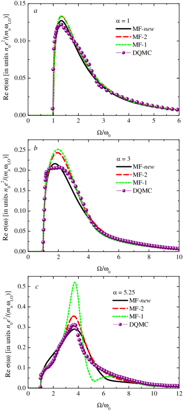
Figure 1: Polaron optical conductivity calculated for $\alpha=1$ (a), $\alpha=3$ (b) and $\alpha=5.25$ (c) within the present non-quadratic MF formalism (denoted in the figure as MF-new), compared with the polaron optical conductivity calculated within the extended memory-function formalism (MF-2) of Ref. PRL2006 , the results of the memory-function approach using the Feynman parabolic trial action DSG (MF-1), and the diagrammatic quantum Monte Carlo (DQMC) M2003 ; PRL2006 .

The subsequent figures show the results for increasing $\alpha$. In Figure 1, the optical conductivity is shown for small coupling, $\alpha=1,$and for $\alpha=3,5.25$ which correspond to the dynamic regime where the RES starts to play a role. In this regime, analytic solutions are provided by the various memory function formalisms listed above, and we compare them to DQMC numeric data M2003 . At weak coupling ($\alpha=1\,,$ panel (a)$)$, all the approaches based on the memory function give results in agreement with DQMC. For $\alpha=3$ (panel (b)), the current method gives a better fit to the DQMC result that the other two methods. For a stronger coupling, $\alpha=5.25$ (panel (c)) the MF-2 approach substantially improves the original result MF-1, but the optical conductivity spectrum calculated within the new non-quadratic MF formalism lies closer to the DQMC data than either of the other two.

Fig. 2 demonstrates the behavior of the polaron optical conductivity spectra in the intermediate coupling regime, for $\alpha=6.5$ and $\alpha=7$. In this regime, the existing memory function approaches (MF-1,MF-2) as well as the existing strong coupling expansions (SCE-1,SCE-2) do not provide satisfactory results. The new memory function approach and the new strong coupling expansion are in much better agreement with the DQMC data.

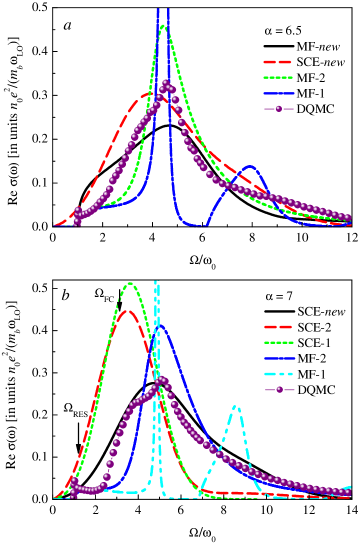
Figure 2: Polaron optical conductivity calculated for $\alpha=6.5$ (a) and $\alpha=7$ (b) using different analytic approaches: the non-quadratic MF formalism (MF-new), the extended memory-function formalism of Ref. PRL2006 (MF-2), the memory-function approach with the Feynman parabolic trial action DSG (MF-1), the non-adiabatic strong-coupling expansion (denoted at the figure as SCE-new), the adiabatic strong-coupling expansions of Refs. PRL2006 ; PRB2014 (SCE-1 and SCE-2). The results are compared to DQMC data of Refs. M2003 ; PRL2006 .

This range of coupling parameters is where one would want to cross over from using a memory function based approach to a strong coupling expansion. Whereas the existing methods do not allow to bridge this gap at intermediate coupling, the extensions that we have proposed here are suited to implement such a cross-over. The present memory-function approach with the non-parabolic trial action leads to a relatively small extension of the range of $\alpha$ where the polaron optical conductivity compares well with the DQMC data, namely from $\alpha\approx 4.5$ to $\alpha\approx 6.5$. For $\alpha\lessapprox 6.5$, the memory-function approach with the non-parabolic trial action provides a better agreement with DQMC than all other known approximations. Remarkably, the optical conductivity spectra as given by the non-quadratic MF formalism and the non-adiabatic SCE are both in better agreement with the Monte Carlo data than any of the preceding analytical methods. For $\alpha=6.5$, the polaron optical conductivity calculated within non-quadratic MF formalism and the non-adiabatic SCE lie rather close to each other. We can conclude therefore that the ranges of validity of those two approximations overlap, despite the fact that these approximations are based on different assumptions.

The maximum of the optical conductivity spectrum provided by the non-quadratic MF formalism for $\alpha=6.5$ is positioned at slightly lower frequency than that for the maximum of the optical conductivity obtained in the strong coupling approximation with non-adiabatic corrections. They lie remarkably close to two features of the DQMC optical conductivity spectrum: the higher-frequency peak, which is the maximum of the spectrum, and the lower-frequency shoulder. The similar comparative behavior of the memory-function and strong coupling results was noticed in Ref. PRL2006 , where it was suggested that these two features in the DQMC spectra can correspond physically to the dynamic (RES) and the Franck-Condon contributions. The present results are in line with that physical picture.

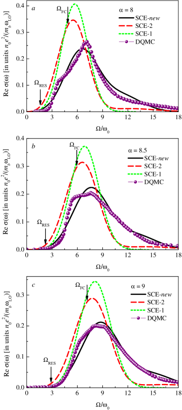
Figure 3: Polaron optical conductivity calculated for $\alpha=8$ (a), $\alpha=8.5$ (b) and $\alpha=9$ (c) within several analytic strong coupling approaches and compared to DQMC data of Refs. M2003 ; PRL2006 . The notations are the same as in Fig. 2.

In Fig. 2 (b), the arrows indicate the FC transition frequency for the transition to the first excited FC state $\Omega_{1,0}\equiv\Omega_{\mathrm{FC}}$ and the RES transition frequency $\Omega_{\mathrm{RES}}$ for a strong coupling polaron as calculated in Ref. KED1969 . We can see that both the shape and the position of the maximum of the optical conductivity band obtained within the adiabatic approximation in Refs. PRL2006 ; PRB2014 are rather far from those for the DQMC data. Taking into account non-adiabatic transitions drastically improves the agreement of the strong coupling approximation with DQMC, even for $\alpha=7$, which, strictly speaking, is not yet the strong coupling regime. The value $\alpha=7$ can be rather estimated as an intermediate coupling. However, even at this intermediate coupling strength, the results of present approach lie much closer to the DQMC data than those obtained within all other aforesaid analytic methods. Also a substantial improvement of the agreement between the strong coupling expansion and DQMC is clearly expressed in Fig. 3, where the polaron optical conductivity spectra are shown for the strong coupling regime for $\alpha=8$ to $\alpha=9$. For strong couplings, the non-adiabatic SCE accurately reproduces both the peak position and the overall shape of the DQMC spectra. Finally, we see that the results of the non-adiabatic SCE remain accurate also in the extremely strong coupling regime, as shown in Fig. 4.

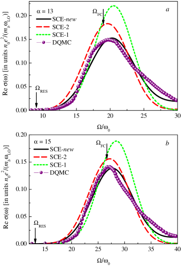
Figure 4: Polaron optical conductivity in the extremely strong coupling regime, for $\alpha=13$ (a) and $\alpha=15$ (b). The notations are the same as in Fig. 2.

IV Conclusions

In the present work, we have modified two basic analytic methods for the polaron optical conductivity in order to extend their ranges of applicability for the electron-phonon coupling constant in such a way that these ranges overlap. The memory function formalism using a trial action for a model two-particle system has been extended to work with non-quadratic interaction potentials in the model system. This method combines the translation invariance of the trial system, which is one of the main advantages of the Feynman variational approach, with a more realistic interaction between the electron and the fictitious particle. This extension leads to a substantial improvement of the polaron optical conductivity for small and intermediate coupling strengths with respect to the preceding known versions of the memory function approach.

The other method is the strong-coupling expansion, and we have extended it beyond the Franck-Condon adiabatic approximation by taking into account non-adiabatic transitions between different excited polaron states. As a result, the modified non-adiabatic strong-coupling expansion appears now to be in good agreement with the numerical DQMC data in a wide range of $\alpha$ from intermediate coupling strength to the strong coupling limit. For the intermediate coupling value $\alpha=6.5$, the two methods that we propose, i.e. the non-quadratic MF formalism and the non-adiabatic SCE, result in optical conductivity spectra which are remarkably close to each other and to the DQMC results. Thus, both methods can be combined to provide all-coupling, accurate analytic results for the polaron optical absorption.

For larger $\alpha$ the agreement between the results of the non-adiabatic SCE and DQMC becomes gradually better. At very strong coupling, even the preceding adiabatic SCE PRB2014 is already sufficiently good, so that the improvement due to the non-adiabatic transitions, e. g., for $\alpha=15$, is relatively small. However, for a slightly weaker coupling, e. g., for $\alpha=9$, we can observe a drastically improved agreement with DQMC for the present non-adiabatic SCE as compared to the adiabatic approximation. We can conclude that at present, the strong coupling approximation taking into account non-adiabatic contributions provides the best agreement with the DQMC results for $\alpha\gtrapprox 6.5$ with respect to all other known analytic approaches for the polaron optical conductivity. We find that the non-adiabatic transitions lead to a substantial change of the spectral shape with respect to the optical conductivity derived within the adiabatic approximation. The non-adiabatic effects are non-negligible in the whole range of the coupling strength, at least for $\alpha\leq 15$, available for DQMC.

In summary, extending the MF and SCE formalisms leads to an overlapping of the areas of $\alpha$ where these two analytic methods are applicable. These analytic methods have been verified, appearing to be in good agreement with numeric DQMC data at all $\alpha$ available for DQMC. We therefore possess the analytic description of the polaron optical response which embraces the whole range of the coupling strength.

- (1) L. D. Landau, Phys. Z. Sowjetunion 3, 664 (1933) [English translation in Collected Papers, Gordon and Breach, New York, 1965, pp. 67-68].
- (2) A. S. Alexandrov and J. T. Devreese, Advances in Polaron Physics (Springer, 2009).
- (3) R. von Helmolt, J. Wecker, B. Holzapfel, L. Schultz, and K. Samwer, Phys. Rev. Lett. 71, 2331 (1993).
- (4) H. Sirringhaus et al., Nature (London) 401, 685 (1999).
- (5) T. Holstein, Ann. Phys. (N.Y.) 8, 325 (1959).
- (6) M. Setvin, C. Franchini, X. Hao, M. Schmid, A. Janotti, M. Kaltak, C. G. Van de Walle, G. Kresse, and U. Diebold, Phys. Rev. Lett. 113, 086402 (2014).
- (7) X. Hao, Z. Wang, M. Schmid, U. Diebold, and C. Franchini, Phys. Rev. B 91, 085204 (2015).
- (8) J. Vlietinck, W. Casteels, K. Van Houcke, J. Tempere, J. Ryckebusch, and J. T. Devreese, New J. Phys. 17, 033023 (2015).
- (9) W. Meevasana, X. J. Zhou, B. Moritz, C.-C. Chen, R. H. He, S.-I. Fujimori, D. H. Lu, S.-K. Mo, R. G. Moore, F. Baumberger, T. P. Devereaux, D. van der Marel, N. Nagaosa, J. Zaanen and Z.-X. Shen, New Journal of Physics 12, 023004 (2010).
- (10) J. L. M. van Mechelen, D. van der Marel, C. Grimaldi, A. B. Kuzmenko, N. P. Armitage, N. Reyren, H. Hagemann, and I. I. Mazin, Phys. Rev. Lett. 100, 226403 (2008).
- (11) J. T. Devreese, S. N. Klimin, J. L. M. van Mechelen, and D. van der Marel, Phys. Rev. B 81, 125119 (2010).
- (12) A. S. Mishchenko, N. V. Prokof’ev, A. Sakamoto, and B. V. Svistunov, Phys. Rev. B 62, 6317 (2000).
- (13) A. S. Mishchenko, N. Nagaosa, N. V. Prokof’ev, A. Sakamoto, and B. V. Svistunov, Phys. Rev. Lett. 91, 236401 (2003).
- (14) G. L. Goodvin, A. S. Mishchenko, and M. Berciu, Phys. Rev. Lett. 107, 076403 (2011).
- (15) E. Kartheuser, R. Evrard, and J. Devreese Phys. Rev. Lett. 22, 94-97 (1969).
- (16) J. Devreese, J. De Sitter, and M. Goovaerts, Phys. Rev. B 5, 2367 (1972).
- (17) J. T. Devreese, in Polarons in Ionic Crystals and Polar Semiconductors (North-Holland, Amsterdam, 1972), pp. 83 – 159.
- (18) G. De Filippis, V. Cataudella, A. S. Mishchenko, C. A. Perroni, and J. T. Devreese, Phys. Rev. Lett. 96, 136405 (2006).
- (19) V. L. Gurevich, I. G. Lang, and Yu. A. Firsov, Sov. Phys. Solid State 4, 918 (1962).
- (20) J. Devreese, W. Huybrechts, and L. Lemmens, Phys. Status Solidi B 48, 77 (1971).
- (21) S. N. Klimin and J. T. Devreese, Phys. Rev. B 89, 035201 (2014).
- (22) R. P. Feynman, R. W. Hellwarth, C. K. Iddings, and P. M. Platzman, Phys. Rev. 127, 1004 (1962).
- (23) R. P. Feynman, Phys. Rev. 97, 660 (1955).
- (24) D. Sels and F. Brosens, Phys. Rev. E 89, 012124 (2014).
- (25) D. Sels and F. Brosens, Phys. Rev. E 89, 042110 (2014).
- (26) D. Sels, arXiv:1605.04998 (2016).
- (27) V. Cataudella, G. De Filippis, and C.A. Perroni, “Single Polaron Properties in Different Electron-Phonon Models”, in: Polarons in Advanced Materials, ed. by A. S. Alexandrov, Springer Series in Materials Science, Volume 103, 2007, pp. 149-189.
- (28) S. N. Klimin and J. T. Devreese, Solid State Communications 151, 144 (2011).
- (29) S. J. Miyake, J. Phys. Soc. Japan 38, 181 (1975).
- (30) S. I. Pekar, Untersuchungen über die Elektronentheorie der Kristalle (Akademie-Verlag, Berlin, 1954).
- (31) G. R. Allcock, in Polarons and Excitons, edited by C. G. Kuper and G. D. Whitfield (Oliver and Boyd, Edinburgh, 1963), pp. 45 – 70.
- (32) A. S. Mishchenko, N. Nagaosa, and N. Prokof’ev, Phys. Rev. Lett. 113, 166402 (2014).
- (33) F. M. Peeters and J. T. Devreese, Phys. Rev. B 28, 6051 (1983).
- (34) R. P. Feynman, Phys. Rev. 84, 108 (1951).