QCD sum rules for the neutron, $\Sigma$, and $\Lambda$ in neutron matter

Abstract

The nuclear density dependencies of the neutron and $\Sigma$ and $\Lambda$ hyperons are important inputs in the determination of the neutron star mass as the appearance of hyperons coming from strong attractions significantly changes the stiffness of the equation of state (EOS) at iso-spin asymmetric dense nuclear matter. In-medium spectral sum rules have been analyzed for the nucleon, $\Sigma$, and $\Lambda$ hyperon to investigate their properties up to slightly above the saturation nuclear matter density by using the linear density approximation for the condensates. The construction scheme of the interpolating fields without derivatives has been reviewed and used to construct a general interpolating field for each baryon with parameters specifying the strength of independent interpolating fields. Optimal choices for the interpolating fields were obtained by requiring the sum rules to be stable against variations of the parameters and the result to be consistent with known phenomenology. The optimized result shows that Ioffe’s choice is not suitable for the $\Lambda$ hyperon sum rules. It is found that, for the $\Lambda$ hyperon interpolating field, the up and down quark combined into the scalar diquark structure $u^{T}C\gamma_{5}d$ should be emphasized to ensure stable sum rules. The quasi-$\Sigma$ and -$\Lambda$ hyperon energies are always found to be higher than the quasineutron energy in the region $0.5<\rho/\rho_{0}<1.5$ where the linear density approximation in the sum-rule analysis is expected to be reliable.

I Introduction

Observations of 2$M_{\odot}$ neutron star Demorest ; Antoniadis sparked a renewed interest for the EOS of dense nuclear matter at large iso-spin asymmetry Fraga:2013qra ; Drago:2014oja ; Drews:2014spa . In the low-density limit, the nuclear matter can be regarded as a gas of weakly interacting quasiparticles filled up to their respective quasi-Fermi sea. In such a limit, the early appearance of the hyperon will make the matter soft because the additional degrees of freedom can be filled in the matter without enhancing the quasi-Fermi sea. Model calculations tend to show that such a soft EOS will not support a 2$M_{\odot}$ neutron star Glendenning:1984jr ; Knorren:1995ds . Therefore, it is generally believed that the hyperon degrees of freedom will eventually become repulsive at high dense matter due to the interactions between nucleon and hyperon, which can lead to a stiff EOS at high nuclear matter density. Even if the nuclear matter is strongly correlated, the appearance of hyperon degrees of freedom usually reduces the energy density of the matter and the maximum mass of the neutron star becomes bounded to values smaller than 2$M_{\odot}$ Glendenning:1984jr ; Knorren:1995ds . Hence, the density behavior of the nucleon as well as the hyperon are of great current interest.

As for the nucleon, the density dependence the quasineutron energy in the asymmetric nuclear matter is characterized by the nuclear symmetry energy Li:2008gp . The nuclear matter energy density will have an additional variation axis if the matter includes a nontrivial fraction of hyperons. Unfortunately, it is hard to calculate the EOS of the dense matter in the hadron phase directly from first principle or from models with relevant effective degrees of freedom because experimental information on these is scare at present. Hopefully, worldwide plans for rare isotope machines that can probe the symmetry energy may improve the situation. Until more experimental data are available, effective method based on quantum chromodynamics (QCD) can be an alternative approach to directly calculate the properties of quasibaryons at high density.

The operator-product-expansion (OPE-based) spectral sum rule (QCD sum rules) is a well established method for investigating the properties of hadrons Shifman:1978bx ; Ioffe:1981kw ; Reinders:1984sr . Through the OPE in QCD degrees of freedom, the nonperturbative QCD contribution at confined phase can be systematically included into the spectral structure of hadron resonance in both the vacuum and nuclear medium. Using theoretical estimates and the results of experimental measurements for the nuclear expectation values of condensates, QCD sum-rules methods have been successfully applied to study nucleons Drukarev:1988kd ; Cohen:1991js ; Furnstahl:1992pi ; Jin:1992id ; Jin:1993up ; Cohen:1994wm and vector mesons Hatsuda:1991ez ; Klingl:1997kf ; Leupold:1997dg ; Klingl:1998sr in the nuclear medium. However, a systematic QCD sum-rule study for the in-medium properties of the $\Sigma$ and $\Lambda$ hyperons using a generalized interpolating fields and updated condensate values is still missing. Although the sum rules have been updated by using some of the condensate values extracted from theoretical development including lattice QCD Alarcon:2012nr ; Ren:2014vea ; Durr:2015dna ; Yang:2015uis , additional assumptions have to be made for the result to be consistent with existing experimental observations from the $\Lambda$ and $\Sigma$ hyper-nuclei Millener:1988hp ; Noumi:2001tx .

In previous studies, the interpolating fields for hyperons have been obtained via SU(3) flavor transformation from the well established Ioffe choice for the nucleon interpolating fields Shifman:1978bx ; Ioffe:1981kw ; Reinders:1984sr ; Jin:1993fr ; Jin:1994bh . But in principle, an independent basis for interpolating fields can be freely constructed as long as it has the required quantum numbers of the hadron of interest. Therefore, the generalized interpolating fields would be a linear combination of the basis set with parameters specifying the strength of the independent basis. An optimal interpolating field will reflect the dominant quark configuration of the ground state and thus have a large overlap with the ground state. If the parameter set are close to the optimal choice, the sum rule would be stable under small variations in the parameters, whereas an unfavorable choice will be reflected in an unstable sum rule.

In this study, we review the construction scheme of the interpolating fields without derivatives for the neutron and $\Sigma$ and $\Lambda$ hyperons and constructed a general interpolating field for each baryon with parameters specifying the strength of independent bases. Optimal choices for the interpolating fields were obtained by requiring the sum rules to be stable against variations of the parameters and the result to be consistent with known phenomenology. The self-energies and the energy of the quasibaryon states and their density behavior have been calculated by the QCD sum-rules approach with the renewed interpolating fields.

This paper is organized as follows: in Sec. II, a brief introduction for in-medium QCD sum rules and arguments for constructing interpolating fields are presented. In Sec. III, detailed OPE for correlation functions are given, and the treatment for in medium condensates are presented. In Sec. IV, the sum rules for the neutron, $\Sigma$, and $\Lambda$ baryons in the neutron matter are analyzed. Discussion and conclusions are given in Sec. V.

II QCD sum rules and interpolating fields

In the Bjorken limit, the scattering amplitude of a hadron and leptons can be calculated by the OPE of the correlation function between explicit quark currents, which overlaps with the partonic configuration in the hadron. This means that the quantum number of a hadron can be interpolated with explicit quark current from the QCD Lagrangian. Moreover, the OPE calculation in the QCD degrees of freedom is justified in this limit. One can also study the properties of a hadron by constructing the corresponding spectral sum rules by using the OPE of the current-current correlation function which contains the hadron state as the ground state. This type of approach is based on the short distance expansion and requires following assumptions:

• The interpolating fields should be constructed to have the quantum number of the hadron of interest and chosen to have a strong overlap with it.

• Among the states that appear in the correlator, the hadron state should be a well separated ground state.

The correlation function of the baryon interpolating fields is defined as

$$\Pi(q)\equiv i\int d^{4}xe^{iqx}\langle\Psi_{0}|\textrm{T}[\eta(x)\bar{\eta}(0)]|\Psi_{0}\rangle,$$ (1)

where $\eta(x)$ is an interpolating field for the baryon and $|\Psi_{0}\rangle$ is the parity and time-reversal symmetric ground state, either of the vacuum or the medium. In the medium case, the state is characterized by its density $\rho=\rho_{n}+\rho_{p}$, the matter velocity $u_{\mu}$, and the iso-spin asymmetry factor $I=(\rho_{n}-\rho_{p})/(\rho_{n}+\rho_{p})$. With assumed parity, time-reversal symmetry, and Lorentz covariance, the correlation function can be decomposed into three invariants Furnstahl:1992pi :

$$\Pi(q)\equiv\Pi_{s}(q^{2},qu)+\Pi_{q}(q^{2},qu)/q+\Pi_{u}(q^{2},qu)/u.$$ (2)

The medium is taken to be at rest; $u^{\mu}\rightarrow(1,\vec{0})$ and $\Pi_{i}(q^{2},qu)\rightarrow\Pi_{i}(q_{0},|\vec{q}|\rightarrow\textrm{fixed})$. Each invariant satisfies the following dispersion relation on the complex $\omega$ plane:

$$\Pi_{i}(q_{0},|\vec{q}|) =\frac{1}{2\pi i}\int^{\infty}_{-\infty}d\omega\frac{\Delta\Pi_{i}(\omega,|\vec{q}|)}{\omega-q_{0}}+F_{n}(q_{0},|\vec{q}|),$$ (3)

where $F_{n}(q_{0},|\vec{q}|)\equiv F^{e}_{n}(q_{0}^{2},|\vec{q}|)+q_{0}F^{o}_{n}(q_{0}^{2},|\vec{q}|)$ is a finite-order polynomial. The discontinuity $\Delta\Pi_{i}(\omega,|\vec{q}|)$ can be defined as follows:

$$\Delta\Pi_{i}(\omega,|\vec{q}|) \equiv\lim_{\epsilon\rightarrow 0^{+}}[\Pi_{i}(\omega+i\epsilon,|\vec{q}|)-\Pi_{i}(\omega-i\epsilon,|\vec{q}|)]=2i\textrm{Im}[\Pi_{i}(\omega+i\epsilon,|\vec{q}|)]$$

$$=\Delta\Pi^{e}_{i}(\omega^{2},|\vec{q}|)+\omega\Delta\Pi^{o}_{i}(\omega^{2},|\vec{q}|).$$ (4)

All the possible resonances including the ground state (quasibaryon pole) are contained in the discontinuity (4). By using these relations, the invariants can be decomposed into an even and an odd part of $q_{0}$, where each part has the following dispersion relation at fixed $|\vec{q}|$:

$$\Pi_{i}(q_{0},|\vec{q}|) =\Pi_{i}^{e}(q_{0}^{2},|\vec{q}|)+q_{0}\Pi_{i}^{o}(q_{0}^{2},|\vec{q}|),$$ (5)

$$\Pi_{i}^{e}(q_{0}^{2},|\vec{q}|) =\frac{1}{2\pi i}\int^{\infty}_{-\infty}d\omega\frac{\omega^{2}}{\omega^{2}-q_{0}^{2}}\Delta\Pi^{o}_{i}(\omega^{2},|\vec{q}|)+F^{e}_{n}(q_{0}^{2},|\vec{q}|),$$ (6)

$$\Pi_{i}^{o}(q_{0}^{2},|\vec{q}|) =\frac{1}{2\pi i}\int^{\infty}_{-\infty}d\omega\frac{1}{\omega^{2}-q_{0}^{2}}\Delta\Pi^{e}_{i}(\omega^{2},|\vec{q}|)+F^{o}_{n}(q_{0}^{2},|\vec{q}|),$$ (7)

where $\Delta\Pi_{i}^{e}(q_{0}^{2},|\vec{q}|)$ and $\Delta\Pi_{i}^{o}(q_{0}^{2},|\vec{q}|)$ are even functions of $q_{0}$.

If one regards the baryon in the nuclear medium as a quasiparticle state, the nuclear interaction can be accounted for as the in-medium self-energies within the mean-field potential. The phenomenological structure of the correlation function near the quasibaryon pole can then be suggested as

$$\Pi(q) \Rightarrow\frac{\lambda^{*2}}{/q-M_{B}-\Sigma(q)}=\lambda^{*2}\frac{/q+M_{B}^{*}-\Sigma_{v}/u}{(q_{0}-E_{q})(q_{0}-\bar{E}_{q})},$$ (8)

where $\Sigma(q)=\Sigma_{s}(q^{2},qu)+\Sigma_{v}(q)/u$, $M_{B}^{*}=M_{B}+\Sigma_{s}(q^{2},qu)$, $E_{q}=\Sigma_{v}+(\vec{q}^{2}+M_{B}^{*2})^{\frac{1}{2}}$, $\bar{E}_{q}=\Sigma_{v}-(\vec{q}^{2}+M_{B}^{*2})^{\frac{1}{2}}$ and $\lambda^{*}$ is the residue at the quasibaryon pole, which accounts for the overlap between the interpolating fields and the quasi-baryon state. The invariants can then be identified as follows:

$$\Pi_{s}(q_{0},|\vec{q}|) =-\lambda^{*2}\frac{M_{B}^{*}}{(q_{0}-E_{q})(q_{0}-\bar{E}_{q})}+\cdots,$$ (9)

$$\Pi_{q}(q_{0},|\vec{q}|) =-\lambda^{*2}\frac{1}{(q_{0}-E_{q})(q_{0}-\bar{E}_{q})}+\cdots,$$ (10)

$$\Pi_{u}(q_{0},|\vec{q}|) =\lambda^{*2}\frac{\Sigma_{v}}{(q_{0}-E_{q})(q_{0}-\bar{E}_{q})}+\cdots.$$ (11)

On the other hand, the invariants can be expressed in terms of QCD degrees of freedom by OPE in following limit: $q^{2}\rightarrow-\infty$, $|\vec{q}|\rightarrow\textrm{fixed}$ (equivalent to $q_{0}^{2}\rightarrow-\infty$, $|\vec{q}|\rightarrow\textrm{fixed}$):

$$\Pi_{i}(q^{2},q_{0}^{2}) =\sum_{n}C^{i}_{n}(q^{2},q_{0}^{2})\langle\hat{O}_{n}\rangle_{\rho,I},$$ (12)

where $C^{i}_{n}(q^{2},q_{0}^{2})$ are the Wilson coefficients, and the condensate part $\langle\hat{O}_{n}\rangle_{\rho,I}$ has been evaluated within the linear density approximation.

Depending on the quantum number and the intrinsic structure of the ground-state hadron, construction of the interpolating fields should be different. In the following section, we argue that while Ioffe’s choice can be suitable for describing the nucleon and $\Sigma$ hyperon family, it is not so for the $\Lambda$ hyperon.

II.1 Interpolating fields for the $\Sigma$ hyperon

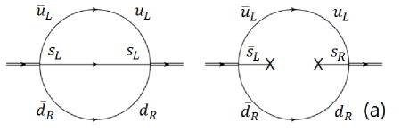
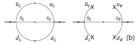
Figure 1: Diagrammatic description for the $\Sigma^{0}$ correlation function. Set (a) shows the self correlation function of basis (16). Set (b) shows the self correlation function of basis (17). In each set, the left diagram shows the partonic propagation over short distance and the right diagram shows the possible lowest dimensional quark condensate contribution. Only strange quarks can propagate to the different helicity state from the initial helicity state.

For the baryon interpolating fields, the most simple structure can be composed by a diquark without derivatives and an attached external quark that carries the fermionic nature of the baryon. If one requires the diquarks to be composed of light quarks without any derivatives, they can be classified into either the iso-spin-asymmetric ($I=0$) or -symmetric ($I=1$) configuration. The set of interpolating fields with the diquark in $I=0$ configuration can be written as follows:

$$\left\{q_{1},q_{2}~{}\textrm{in}~{}I=0\right\}=\left\{\epsilon_{abc}[q_{1a}^{T}Cq_{2b}]\gamma_{5}q_{3c},~{}\epsilon_{abc}[q_{1a}^{T}C\gamma_{5}q_{2b}]q_{3c},~{}\epsilon_{abc}[q_{1a}^{T}C\gamma_{5}\gamma_{\mu}q_{2b}]\gamma^{\mu}q_{3c}\right\},$$ (13)

where $q_{1}$ and $q_{2}$ stand for the light quark flavors and $q_{3}$ stands for the external quark flavor. The set for $I=1$ configuration can be written as follows:

$$\left\{q_{1},q_{2}~{}\textrm{in}~{}I=1\right\}=\left\{\epsilon_{abc}[q_{1a}^{T}C\gamma_{\mu}q_{2b}]\gamma_{5}\gamma^{\mu}q_{3c},~{}\epsilon_{abc}[q_{1a}^{T}C\sigma_{\mu\nu}q_{2b}]\gamma_{5}\sigma^{\mu\nu}q_{3c}\right\}.$$ (14)

Hence, for the $\Sigma$ family, the interpolating fields can be expressed as linear combinations of the bases in the set (14) with $q_{3}$ taken to be the external strange quark flavor.

On the other hands, the interpolating fields can also be constructed by requiring (i) the diquark structure in the $s=0$ configuration without any derivative and (ii) the light quarks in the $I=1$ configuration. Either way, the most general lowest dimensional interpolating fields for the $\Sigma$ can be written as follows:

$$\eta_{\Sigma(t)} =\epsilon_{abc}\left([q^{T}_{1a}Cs_{b}]\gamma_{5}q_{2c}+[q^{T}_{2a}Cs_{b}]\gamma_{5}q_{1c}+t\left([q^{T}_{1a}C\gamma_{5}s_{b}]q_{2c}+[q^{T}_{2a}C\gamma_{5}s_{b}]q_{1c}\right)\right)$$

$$=\left(\frac{1-t}{2}\right)\epsilon_{abc}[q^{T}_{1a}C\gamma_{\mu}q_{2b}]\gamma_{5}\gamma^{\mu}s_{c}+\left(\frac{1+t}{4}\right)\epsilon_{abc}[q^{T}_{1a}C\sigma_{\mu\nu}q_{2b}]\gamma_{5}\sigma^{\mu\nu}s_{c},$$ (15)

where Fierz rearrangement has been executed to make the diquark parts carry the iso-spin information ($I=1$) and the strange quark carry the spin information ($s=1/2$). In the second line, the independent basis set reduced to the set (14). The corresponding fields for $\Sigma^{+}$, $\Sigma^{0}$, and $\Sigma^{-}$ can be obtained by choosing $q_{1}$ and $q_{2}$ for the appropriate light quark flavor. After choosing $q_{1}=u$ and $q_{2}=d$ for $\Sigma^{0}$, each basis can be expressed in the helicity states:

$$\epsilon_{abc}[u^{T}_{a}C\gamma_{\mu}d_{b}]\gamma_{5}\gamma^{\mu}s_{c} =2\epsilon_{abc}\left([u^{T}_{R,a}Cs_{R,b}]d_{L,c}+[d^{T}_{R,a}Cs_{R,b}]u_{L,c}-(L\leftrightarrow R)\right),$$ (16)

$$\epsilon_{abc}[u^{T}_{a}C\sigma_{\mu\nu}d_{b}]\gamma_{5}\sigma^{\mu\nu}s_{c} =4\epsilon_{abc}\left([u^{T}_{R,a}Cs_{R,b}]d_{R,c}+[d^{T}_{R,a}Cs_{R,b}]u_{R,c}-(L\leftrightarrow R)\right),$$ (17)

where the subscripts $L$ and $R$ denote the left- and right-helicity states, respectively.

Both bases can contribute to the short-ranged partonic propagation (perturbative contribution). On the other hand, if one tries to include the long-ranged correlation (nonperturbative contribution), then the second basis (17) may have a problem at the lowest order. To understand this issue consider the propagation between two helicity states. Near the separation scale of the OPE, for which the mass scale of the low-lying baryon ($\sim 1~{}\textrm{GeV}$) is taken, the light quark mass is negligible. Hence, for the light quarks, the perturbative propagation preserves helicity. However, because the strange quark mass is non-negligible compared with the separation scale, the strange quark propagation can mix helicity: the helicity mixing part is proportional to the strange quark mass. In the nonperturbative regime, the leading chiral symmetry-breaking term occurs as $\langle\bar{q}_{L}q_{R}\rangle$ or $\langle\bar{q}_{R}q_{L}\rangle$, hence occurs only between correlations of mixed helicity. This mechanism explains the origin of the vacuum baryon masses Ioffe:1981kw and has the following effect for the correlation function:

In the OPE of the self correlation function of the basis (16), the lowest dimensional quark condensate is $\langle\bar{s}s\rangle$ [Fig. 1(a)]. The medium part of $\langle\bar{s}s\rangle$ can be estimated in the linear density approximation with recent lattice QCD studies Durr:2015dna ; Yang:2015uis . However, as one can see in Fig. 1(b), in the OPE of the self-correlation function of the basis (17), the four-quark condensates, whose matrix element is still not known well, appear as the lowest-dimensional quark condensate. The cross correlation function between basis (16) and (17) also cannot have two-quark condensate as the lowest mass dimensional term. If one knows the value of dimension-6 four-quark condensates, inclusion of basis (17) will not be any problem, because the physical results should not depend on the choice of the basis. However, because we have only limited constraints to the four-quark condensates, the uncertainty of these expectation values will be amplified if they appear as the leading quark operator. Setting $t=-1$ (Ioffe’s choice), one can suppress the contribution from the self-correlation function of basis (17) and consequently avoid the problem.

In Ioffe’s interpolating fields (16), the diquark structure is a pseudovector $u^{T}C\gamma_{\mu}d$ ($s^{P}=0^{-}$ for $\mu=0$, $s^{P}=1^{+}$ for $\mu=i$). In spatial rotation, the time component behaves as a scalar ($s=0$) and spatial components behave as a three-vector ($s=1$). Therefore, the relative angular momentum between the light quarks in the nonrelativistic quasi-$\Sigma$ state described through the basis (16) should be in the $l=1$ state.

II.2 Interpolating fields for the nucleon

A similar argument can be made for the nucleon case. In this case, the most simple structure would be composed by (i) the diquark in $I=0$ configuration and (ii) an attached external quark which carries the fermionic nature and iso-spin of the nucleon. The linear combination can be written as

$$\eta_{N(t_{1},t_{2})} =\epsilon_{abc}\left([q_{1a}^{T}Cq_{2b}]\gamma_{5}q_{3c}+t_{1}[q_{1a}^{T}C\gamma_{5}q_{2b}]q_{3c}+t_{2}[q_{1a}^{T}C\gamma_{5}\gamma_{\mu}q_{2b}]\gamma^{\mu}q_{3c}\right),$$ (18)

where the light quark flavors $q_{1}$ and $q_{2}$ are in $I=0$ configuration and $q_{3}=u$ ($q_{3}=d$) for the proton (neutron). In the nucleon case, $q_{1}=q_{3}\neq q_{2}$ or $q_{2}=q_{3}\neq q_{1}$ and the light quarks with the same flavor should be in the $I=1$ configuration: the third basis in the interpolating field (18) can be rearranged as

$$\epsilon_{abc}[q_{1a}^{T}C\gamma_{5}\gamma_{\mu}q_{2b}]\gamma^{\mu}q_{1c}=-\frac{1}{2}\epsilon_{abc}[q_{1a}^{T}C\gamma_{\mu}q_{1b}]\gamma_{5}\gamma^{\mu}q_{2c}=-\epsilon_{abc}\left([q_{1a}^{T}Cq_{2b}]\gamma_{5}q_{1c}-[q_{1a}^{T}C\gamma_{5}q_{2b}]q_{1c}\right),$$ (19)

so that the number of independent bases in the interpolating fields (18) has been reduced to two:

$$\eta_{N(t)} =2\epsilon_{abc}\left([q_{1a}^{T}Cq_{2b}]\gamma_{5}q_{1c}+t[q_{1a}^{T}C\gamma_{5}q_{2b}]q_{1c}\right)$$

$$=\left(\frac{1-t}{2}\right)\epsilon_{abc}[q_{1a}^{T}C\gamma_{\mu}q_{1b}]\gamma_{5}\gamma^{\mu}q_{2c}+\left(\frac{1+t}{4}\right)\epsilon_{abc}[q_{1a}^{T}C\sigma_{\mu\nu}q_{1b}]\gamma_{5}\sigma^{\mu\nu}q_{2c}.$$ (20)

After choosing $q_{1}=u$ and $q_{2}=d$ for the proton interpolating fields, each basis can be expressed as follows:

$$\epsilon_{abc}[u^{T}_{a}C\gamma_{\mu}u_{b}]\gamma_{5}\gamma^{\mu}d_{c} =4\epsilon_{abc}\left([u^{T}_{R,a}Cd_{R,b}]u_{L,c}-[u^{T}_{L,a}Cd_{L,b}]u_{R,c}\right),$$ (21)

$$\epsilon_{abc}[u^{T}_{a}C\sigma_{\mu\nu}u_{b}]\gamma_{5}\sigma^{\mu\nu}d_{c} =4\epsilon_{abc}\left([u^{T}_{R,a}Cd_{R,b}]u_{R,c}-[u^{T}_{L,a}Cd_{L,b}]u_{L,c}\right),$$ (22)

where the basis (21) is known as Ioffe’s interpolating fields for nucleons.

In the vacuum, the lowest dimensional quark operator appearing in the OPE of the self-correlation function of basis (22), which can also be obtained from taking $t=1$ in Eq. (20), starts from the dimension-9 six-quark condensate term, whose Wilson coefficient comes from perturbative gluon attachment for the external momentum flow with all quarks disconnected. On the other hand, for the self-correlation function of the basis (21), obtained by taking $t=-1$, the OPE starts from the dimension-3 chiral condensate. Hence, as we do not know the exact value of the six-quark condensate and the $\alpha_{s}$ is sensitive to subtraction scale ($\sim 1~{}\textrm{GeV}$), a reliable OPE can be obtained in the vacuum by choosing the basis (21) (Ioffe’s choice). In the medium, the dimension-3 quark density operator appears in the OPE for both currents. However, we retain the vacuum choice for the basis because we want to build the correction from the medium starting from a reliable vacuum OPE. As in the case of $\Sigma$, the diquark structure in Ioffe’s choice (21) is a pseudovector $q^{T}C\gamma_{\mu}q$ ($s^{P}=0^{-}$ for $\mu=0$, $s^{P}=1^{+}$ for $\mu=i$), where $q$ is $u$ for the proton and $d$ for the neutron.

It is generally believed that the most attractive diquark is the scalar channel $\epsilon_{abc}[u^{T}_{a}C\gamma_{5}d_{b}]$. However, because this channel is in the iso-spin asymmetric combination, it can not occur in the $\Sigma$ channel. Also, in the proton channel, the $ud$ diquark could be either in $I=0$ or $I=1$. This fact is in stark contrast to the $\Lambda$ case, where its $ud$ quantum number can be identified with the most attractive channel. As we will see, sum-rule analysis indeed favors the dominance of the most attractive diquark channel for the $\Lambda$ interpolating fields.

II.3 Interpolating fields for the $\Lambda$ hyperon

For the $\Lambda$ hyperon, the basis set can be taken just for the set (13) with $q_{3}=s$. One can try another approach by requiring the following conditions: (i) the diquarks in the $s=0$ configuration and (ii) the light quarks in $I=0$ configuration. The following basis set can then be considered:

$$\left\{\epsilon_{abc}[u^{T}_{a}Cd_{b}]\gamma_{5}s_{c},~{}\epsilon_{abc}[u^{T}_{a}C\gamma_{5}d_{b}]s_{c},~{}\epsilon_{abc}\left([u^{T}_{a}Cs_{b}]\gamma_{5}d_{c}-[d^{T}_{a}Cs_{b}]\gamma_{5}u_{c}\right),~{}\epsilon_{abc}\left([u^{T}_{a}C\gamma_{5}s_{b}]d_{c}-[d^{T}_{a}C\gamma_{5}s_{b}]u_{c}\right)\right\}.$$ (23)

Using the Fierz rearrangement, the third and fourth basis can be rearranged as

$$\epsilon_{abc}\left([u^{T}_{a}Cs_{b}]\gamma_{5}d_{c}-[d^{T}_{a}Cs_{b}]\gamma_{5}u_{c}\right) =\frac{1}{2}\epsilon_{abc}\left([u^{T}_{a}Cd_{b}]\gamma_{5}s_{c}+[u^{T}_{a}C\gamma_{5}d_{b}]s_{c}-[u^{T}_{a}C\gamma_{5}\gamma_{\mu}d_{b}]\gamma^{\mu}s_{c}\right),$$ (24)

$$\epsilon_{abc}\left([u^{T}_{a}C\gamma_{5}s_{b}]d_{c}-[d^{T}_{a}C\gamma_{5}s_{b}]u_{c}\right) =\frac{1}{2}\epsilon_{abc}\left([u^{T}_{a}Cd_{b}]\gamma_{5}s_{c}+[u^{T}_{a}C\gamma_{5}d_{b}]s_{c}+[u^{T}_{a}C\gamma_{5}\gamma_{\mu}d_{b}]\gamma^{\mu}s_{c}\right).$$ (25)

Hence, the basis set (23) can be reduced to the set (13) with $q_{3}=s$:

$$\{\epsilon_{abc}[u^{T}_{a}Cd_{b}]\gamma_{5}s_{c},~{}\epsilon_{abc}[u^{T}_{a}C\gamma_{5}d_{b}]s_{c},~{}\epsilon_{abc}[u^{T}_{a}C\gamma_{5}\gamma_{\mu}d_{b}]\gamma^{\mu}s_{c}\}.$$ (26)

The generalized interpolating fields can then be written as follows:

$$\eta_{\Lambda(\tilde{a},\tilde{b})} =A_{(\tilde{a},\tilde{b})}\epsilon_{abc}\left([u^{T}_{a}Cd_{b}]\gamma_{5}s_{c}+\tilde{a}[u^{T}_{a}C\gamma_{5}d_{b}]s_{c}+\tilde{b}[u^{T}_{a}C\gamma_{5}\gamma_{\mu}d_{b}]\gamma^{\mu}s_{c}\right),$$ (27)

where $A_{(\tilde{a},\tilde{b})}$ is an overall normalization constant. As the self-energies will be obtained by taking the ratios of Borel transformed invariants, the overall normalization becomes irrelevant and the free parameters can be reduced to $\tilde{a}$ and $\tilde{b}$. The basis set can be written in terms of helicity states:

$$\epsilon_{abc}[u^{T}_{a}Cd_{b}]\gamma_{5}s_{c} =\epsilon_{abc}\left([u^{T}_{R,a}Cd_{R,b}]s_{R,c}-[u^{T}_{R,a}Cd_{R,b}]s_{L,c}-(L\leftrightarrow R)\right),$$ (28)

$$\epsilon_{abc}[u^{T}_{a}C\gamma_{5}d_{b}]s_{c} =\epsilon_{abc}\left([u^{T}_{R,a}Cd_{R,b}]s_{R,c}+[u^{T}_{R,a}Cd_{R,b}]s_{L,c}-(L\leftrightarrow R)\right),$$ (29)

$$\epsilon_{abc}[u^{T}_{a}C\gamma_{5}\gamma_{\mu}d_{b}]\gamma^{\mu}s_{c} =2\epsilon_{abc}\left([u^{T}_{R,a}Cs_{R,b}]d_{L,c}-[d^{T}_{R,a}Cs_{R,b}]u_{L,c}-(L\leftrightarrow R)\right).$$ (30)

If one changes the $I=0$ combination on the right-hand side of basis (30) to the $I=1$ combination, the basis changes into Ioffe’s choice for the $\Sigma$ family (16). The light quark condensate only appears in the cross correlation function between bases (29) and (30). The lowest dimensional quark condensates in the self-correlation function of each basis is $\langle\bar{s}s\rangle$. Hence, determining the parameters in Eq. (27) corresponds to determining the weight of lowest dimensional operators $\langle\bar{q}q\rangle$ and $\langle\bar{s}s\rangle$ in the OPE of the correlation function.

The commonly used interpolating fields for $\Lambda$, called Ioffe’s choice, can be obtained by choosing $\{\tilde{a},\tilde{b}\}=\{-1,-1/2\}$ in Eq. (27):

$$\eta_{\Lambda(-1,-1/2)} \Rightarrow\sqrt{\frac{2}{3}}\epsilon_{abc}\left([u^{T}_{a}C\gamma_{\mu}s_{b}]\gamma_{5}\gamma^{\mu}d_{c}-[d^{T}_{a}C\gamma_{\mu}s_{b}]\gamma_{5}\gamma^{\mu}u_{c}\right),$$ (31)

where the overall normalization $A_{(-1,-1/2)}=\sqrt{8/3}$ has been obtained from SU(3) flavor transformation from Ioffe’s interpolating field for nucleon (21). The choice for $\tilde{a}=-1$ causes large cancellation between the OPE terms in the scalar invariants. The canceled part comes from the self-correlation function of basis (28) and of basis (29). This means that, in studies where the Ioffe’s choice (31) were used, a large portion of the scalar invariant $\Pi_{s}(q_{0},|\vec{q}|)$ comes from the self-correlation function of basis (30). In this choice, as can be found in next section, the chiral condensate term has a larger weight than the strange quark condensate and the perturbative contributions, making the OPE less reliable. Moreover, as can be seen in the next section, phenomenological implications strongly suggest that taking a large $\tilde{a}$ and a small $\tilde{b}$ value gives a most efficient sum rule and hence the best choice for the interpolating fields. The argument for determining the stable region in $\{\tilde{a},\tilde{b}\}$ plane will be given in the next sections.

The diquark structure in the bases (28), (29), and (30) are pseudoscalar $u^{T}Cd$ ($s^{P}=0^{-}$), scalar $u^{T}C\gamma_{5}d$ ($s^{P}=0^{+}$) and vector $u^{T}C\gamma_{5}\gamma_{\mu}d$ ($s^{P}=0^{+}$ for $\mu=0$, $s^{P}=1^{-}$ for $\mu=i$) respectively. The corresponding relative angular momentum between the light quarks in the nonrelativistic limit are $l=1$ for pseudoscalar and $l=0$ for scalar and vector diquark.

III Operator Product Expansion and Borel sum rules

In this section, we will list the OPE of the generalized $\Lambda$ correlation function and only the explicit four-quark OPE terms of $\Sigma^{+}$ correlation function. The other OPE terms of the nucleon and $\Sigma^{+}$ correlation function with Ioffe’s choice can be found in Refs. Jeong:2012pa ; Jin:1994bh . Also, covariant derivative expansion and factorization hypothesis have been minimally used.

III.1 Brief summary for the condensates and input parameters

A detailed description for the in-medium light quark and gluon condensates can be found in Refs. Cohen:1991nk ; Furnstahl:1992pi ; Jin:1992id ; Jin:1993up ; Jeong:2012pa . The strange quark condensate can be written as follows:

$$\langle\bar{s}s\rangle_{\rho,I}=\langle\bar{s}s\rangle_{\textrm{vac}}+\langle\bar{s}s\rangle_{p}\rho,$$ (32)

where $\langle\bar{s}s\rangle_{\textrm{vac}}$ is taken to be $(0.8)\langle\bar{q}q\rangle_{\textrm{vac}}$ Shifman:1978bx ; Reinders:1984sr , whereas the medium part can be determined by constraining the parameter $y=\langle\bar{s}s\rangle_{p}/\langle\bar{q}q\rangle_{p}=m_{q}\sigma_{sN}/m_{s}\sigma_{N}$, which represents the strange quark content in the proton. Recent theoretical developments including chiral effective theory Alarcon:2012nr and lattice QCD studies Ren:2014vea ; Durr:2015dna ; Yang:2015uis confine $y\leq 0.2$. We will take $y=0.1$ throughout this work. For nonstrange nuclear matter, $\langle s^{\dagger}s\rangle_{\rho,I}=0$, whereas $\langle s^{\dagger}s\rangle_{\rho,I}$ will be nonzero if hyper-nuclear matter appears at the high density regime. The covariant derivative expansions of the strange quark condensates can be written as

$$\langle s^{\dagger}iD_{0}s\rangle_{\rho,I} =\langle s^{\dagger}iD_{0}s\rangle_{\textrm{vac}}+\langle s^{\dagger}iD_{0}s\rangle_{p}\rho=\frac{m_{s}}{4}\langle\bar{s}s\rangle_{\textrm{vac}}+\left(\frac{m_{s}}{4}\langle\bar{s}s\rangle_{p}+\frac{3}{8}M_{p}A^{s}_{2}\right)\rho,$$ (33)

where $A^{s}_{2}=0.050$ Jin:1993fr .

In this paper, we have changed some definition of the symbols for the four-quark condensates as compared with Refs. Choi:1993cu ; Jeong:2012pa . The new definition can be written as

$$\epsilon_{abc}\epsilon_{a^{\prime}b^{\prime}c}\langle\bar{q}_{1a^{\prime}}\Gamma_{m}^{\alpha}q_{1a}\bar{q}_{2b^{\prime}}\Gamma_{m}^{\beta}q_{2b}\rangle_{\rho,I}= ~{}\frac{1}{4}g^{\alpha\beta}\langle\bar{q}_{1}\Gamma_{m}q_{1}\bar{q}_{2}\Gamma_{m}q_{2}\rangle_{\textrm{tr.}}+\left(u^{\alpha}u^{\beta}-\frac{1}{4}g^{\alpha\beta}\right)\langle\bar{q}_{1}\Gamma_{m}q_{1}\bar{q}_{2}\Gamma_{m}q_{2}\rangle_{\textrm{s.t.}},$$ (34)

$$\langle\bar{q}_{1}\Gamma_{m}q_{1}\bar{q}_{2}\Gamma_{m}q_{2}\rangle_{\textrm{tr.}}= ~{}\frac{2}{3}\langle\bar{q}_{1}\Gamma_{m}^{\alpha}q_{1}\bar{q}_{2}\Gamma_{m\alpha}q_{2}\rangle_{\textrm{vac}}-2\langle\bar{q}_{1}\Gamma_{m}^{\alpha}t^{A}q_{1}\bar{q}_{2}\Gamma_{m\alpha}t^{A}q_{2}\rangle_{\textrm{vac}}$$

$$+\sum_{i=\{n,p\}}\left(\frac{2}{3}\langle\bar{q}_{1}\Gamma_{m}^{\alpha}q_{1}\bar{q}_{2}\Gamma_{m\alpha}q_{2}\rangle_{i}-2\langle\bar{q}_{1}\Gamma_{m}^{\alpha}t^{A}q_{1}\bar{q}_{2}\Gamma_{m\alpha}t^{A}q_{2}\rangle_{i}\right)\rho_{i},$$ (35)

$$\langle\bar{q}_{1}\Gamma_{m}q_{1}\bar{q}_{2}\Gamma_{m}q_{2}\rangle_{\textrm{s.t.}}= ~{}\sum_{i=\{n,p\}}\left(\frac{2}{3}\langle\bar{q}_{1}\Gamma_{m}q_{1}\bar{q}_{2}\Gamma_{m}q_{2}\rangle_{i,\textrm{s.t.}}-2\langle\bar{q}_{1}\Gamma_{m}t^{A}q_{1}\bar{q}_{2}\Gamma_{n}t^{A}q_{2}\rangle_{i,\textrm{s.t.}}\right)\rho_{i},$$ (36)

where $q_{1}$, $q_{2}$ represent the quark flavor, $\Gamma_{m}=\{I,\gamma_{5},\gamma,\gamma_{5}\gamma,\sigma\}$ and each subscript vac, $i$, and s.t. represents the vacuum expectation value, nucleon expectation value, and symmetric traceless matrix element, respectively. Twist-4 matrix elements $\langle\bar{q}_{1}\Gamma_{m}q_{1}\bar{q}_{2}\Gamma_{m}q_{2}\rangle_{i,\textrm{s.t.}}$ and $\langle\bar{q}_{1}\Gamma_{m}t^{A}q_{1}\bar{q}_{2}\Gamma_{m}t^{A}q_{2}\rangle_{i,\textrm{s.t.}}$ can be estimated from DIS data following the arguments presented in Refs. Choi:1993cu ; Jeong:2012pa . For spin-0 and spin-1 operators, the factorization hypothesis has been used:

$$\langle q^{a}_{\alpha}\bar{q}^{b}_{\beta}q^{c}_{\gamma}\bar{q}^{d}_{\delta}\rangle_{\rho,I} \simeq\langle q^{a}_{\alpha}\bar{q}^{b}_{\beta}\rangle_{\rho,I}\langle q^{c}_{\gamma}\bar{q}^{d}_{\delta}\rangle_{\rho,I}-\langle q^{a}_{\alpha}\bar{q}^{d}_{\delta}\rangle_{\rho,I}\langle q^{c}_{\gamma}\bar{q}^{b}_{\beta}\rangle_{\rho,I},$$

$$\langle q1^{a}_{1\alpha}\bar{q}^{b}_{1\beta}q^{c}_{2\gamma}\bar{q}^{d}_{2\delta}\rangle_{\rho,I} \simeq\langle q^{a}_{1\alpha}\bar{q}^{b}_{1\beta}\rangle_{\rho,I}\langle q^{c}_{2\gamma}\bar{q}^{d}_{2\delta}\rangle_{\rho,I}.$$ (37)

This factorization scheme can only be justified in the vacuum and in the large-$N_{c}$ limit. In general, model calculations find large violations depending on the stucture of the four-quark operator GomezNicola:2010tb ; Drukarev:2012av . Therefore, we will introduce the following parametrized form for the medium dependence of the four-quark operators and investigate the result as a function of the parameters that will probe different factorized forms and values for the vacuum and medium part of the four-quark operators separately. After taking the average of color and Dirac index, the remaining scalar condensates have been parametrized as

$$\langle[\bar{q}q]_{u,d}\rangle^{2}_{\rho,I} \Rightarrow k_{1}\langle\bar{q}q\rangle^{2}_{\textrm{vac}}+2f_{1}\left(\langle[\bar{q}q]_{0}\rangle_{p}\mp\langle[\bar{q}q]_{1}\rangle_{p}I\right)\langle\bar{q}q\rangle_{\textrm{vac}}\rho,$$ (38)

$$\langle\bar{u}u\rangle_{\rho,I}\langle\bar{d}d\rangle_{\rho,I} \Rightarrow k_{1}\langle\bar{q}q\rangle^{2}_{\textrm{vac}}+2f_{1}\langle[\bar{q}q]_{0}\rangle_{p}\langle\bar{q}q\rangle_{\textrm{vac}}\rho,$$ (39)

$$\langle\bar{q}q\rangle_{\rho,I}\langle\bar{s}s\rangle_{\rho,I} \Rightarrow k_{2}\langle\bar{q}q\rangle_{\textrm{vac}}\langle\bar{s}s\rangle_{\textrm{vac}}+f_{2}\left(\langle\bar{s}s\rangle_{p}\langle\bar{q}q\rangle_{\textrm{vac}}+\langle[\bar{q}q]_{0}\rangle_{p}\langle\bar{s}s\rangle_{\textrm{vac}}+\langle[\bar{q}q]_{1}\rangle_{p}\langle\bar{s}s\rangle_{\textrm{vac}}I\right)\rho,$$ (40)

where parameters $k_{1}$, $k_{2}$ determine the vacuum strength and $f_{1}$, $f_{2}$ determine the medium dependence of the scalar four-quark condensate. Both $k_{1}$ and $k_{2}$ are set to be 1 as the in-medium sum rules do not show drastic change in the range $0.5\leq k_{1},k_{2}\leq 3.0$ as one can find in Appendix A. According to previously reported studies, $|f_{1}|$ should be weak ($|f_{1}|\ll 1$) Cohen:1994wm ; Jeong:2012pa but $f_{2}$ can be strong ($f_{2}\simeq 1$). This scale difference between the condensates seems reasonable because the strange quark operator only has sea quark contributions in the normal nuclear matter expectation value whereas the light quark operator has additional valence quark contributions. Detailed arguments for the twist-4 matrix elements and the parameter dependencies are presented in Appendix A.

As each quasinucleon has its own quasi-Fermi sea, the external three-momentum of the quasibaryon will be set at the Fermi momentum at the given nuclear matter density: $|\vec{q}|=270~{}\textrm{MeV}$ when $\rho=\rho_{0}=0.16~{}\textrm{fm}^{-3}=(110~{}\textrm{MeV})^{3}$. For the same reason, the external momentum for the quasihyperon will be set to $|\vec{q}|=0~{}\textrm{MeV}$.

The correlation function contains all possible resonances that overlap with the quantum number of the interpolating fields as discussed before. As our interests are the self-energies on the quasibaryon pole, the other excitations should be suppressed. Borel sum rules can be used for this purpose: the weight function $W(\omega)=(\omega-\bar{E}_{q})e^{-\omega^{2}/M^{2}}$ has been applied to the discontinuity in the dispersion relation (3) and the corresponding differential operator $\bar{\mathcal{B}}$ has been applied to the OPE side. Each transformed part will be denoted as $\overline{\mathcal{W}}_{M}[\Pi(q_{0}^{2},|\vec{q}|)]$ and $\bar{\mathcal{B}}[\Pi(q_{0}^{2},|\vec{q}|)]$ respectively. Details for weighting scheme and corresponding differential operation in the Borel sum rules that we use in this work can be found in Refs. Furnstahl:1992pi ; Cohen:1994wm ; Beneke:1994rs ; Beneke:1994sw .

Borel transformed invariants contain the quasi-antipole $\bar{E}_{q}$ as an input parameter. As we are following relativistic-mean-field-type phenomenology, the antipole $\bar{E}_{q}$ is already defined regardless of the actual existence of the pole in the medium. The exact value can be determined by solving the self-consisted dispersion relation:

$$\bar{E}_{q}=\Sigma_{v}(\bar{E}_{q})-\sqrt{\vec{q}^{2}+M^{*}(\bar{E}_{q})^{2}}.$$ (41)

The exact solution of this relation has been used for the antipole value. In density plot, we consider two choices. First, as the quasi-antibaryon excitation may be broadened and may not exist as a pole in the nuclear matter, the value can just be taken as a constant calculated at the saturation nuclear matter density. Second, one can calculate the exact solution of Eq. (41) self consistently at a given density. Because the condensates are approximated with linear density approximation, the sum rule itself and the solution of Eq. (41) are expected to be valid up to densities slightly above the saturation density.

III.2 OPE of the generalized $\Lambda$ correlation function

The OPE of the generalized $\Lambda$ correlation function can be calculated as follows:

$$\Pi^{e}_{\Lambda,s}(q_{0}^{2},|\vec{q}|)= ~{}\frac{(1-\tilde{a}^{2}+2\tilde{b}^{2})}{128\pi^{4}}m_{s}(q^{2})^{2}\ln(-q^{2})$$

$$-\frac{(1-\tilde{a}^{2}+2\tilde{b}^{2})}{16\pi^{2}}q^{2}\ln(-q^{2})\langle\bar{s}s\rangle_{\rho,I}+\frac{\tilde{a}\tilde{b}}{4\pi^{2}}q^{2}\ln(-q^{2})\langle\bar{q}q\rangle_{\rho,I}$$

$$+\frac{(1-\tilde{a}^{2}-2\tilde{b}^{2})}{128\pi^{2}}m_{s}\ln(-q^{2})\left\langle\frac{\alpha_{s}}{\pi}G^{2}\right\rangle_{\rho,I}$$

$$-\frac{(1+\tilde{a}^{2}+4\tilde{b}^{2})}{4}\frac{m_{s}}{q^{2}}\langle\bar{u}u\bar{d}d\rangle_{\textrm{tr.}}-\frac{(1+\tilde{a}^{2}-4\tilde{b}^{2})}{4}\frac{m_{s}}{q^{2}}\langle\bar{u}\gamma_{5}u\bar{d}\gamma_{5}d\rangle_{\textrm{tr.}}+\frac{(1-\tilde{a}^{2}-2\tilde{b}^{2})}{4}\frac{m_{s}}{q^{2}}\langle\bar{u}\gamma u\bar{d}\gamma d\rangle_{\textrm{tr.}}$$

$$+\frac{(1-\tilde{a}^{2}+2\tilde{b}^{2})}{4}\frac{m_{s}}{q^{2}}\langle\bar{u}\gamma_{5}\gamma u\bar{d}\gamma_{5}\gamma d\rangle_{\textrm{tr.}}+\frac{(1+\tilde{a}^{2})}{8}\frac{m_{s}}{q^{2}}\langle\bar{u}\sigma u\bar{d}\sigma d\rangle_{\textrm{tr.}},$$ (42)

$$\Pi^{o}_{\Lambda,s}(q_{0}^{2},|\vec{q}|)= -\frac{(1-\tilde{a}^{2}+2\tilde{b}^{2})}{8\pi^{2}}m_{s}\ln(-q^{2})\langle q^{\dagger}q\rangle_{\rho,I}-\frac{2\tilde{a}\tilde{b}}{3}\frac{1}{q^{2}}\langle q^{\dagger}q\rangle_{\rho,I}\langle\bar{q}q\rangle_{\textrm{vac}}+\frac{(1-\tilde{a}^{2}+4\tilde{b}^{2})}{3}\frac{1}{q^{2}}\langle q^{\dagger}q\rangle_{\rho,I}\langle\bar{s}s\rangle_{\textrm{vac}},$$ (43)

$$\Pi^{e}_{\Lambda,q}(q_{0}^{2},|\vec{q}|)= -\frac{(1+\tilde{a}^{2}+4\tilde{b}^{2})}{512\pi^{4}}(q^{2})^{2}\ln(-q^{2})+\frac{\tilde{a}\tilde{b}}{4\pi^{2}}m_{s}\ln(-q^{2})\langle\bar{q}q\rangle_{\rho,I}-\frac{(1+\tilde{a}^{2}+4\tilde{b}^{2})}{32\pi^{2}}m_{s}\ln(-q^{2})\langle\bar{s}s\rangle_{\rho,I}$$

$$-\frac{(1+\tilde{a}^{2}+4\tilde{b}^{2})}{256\pi^{2}}\ln(-q^{2})\left\langle\frac{\alpha_{s}}{\pi}G^{2}\right\rangle_{\rho,I}$$

$$+\frac{(1-\tilde{a}^{2}+2\tilde{b}^{2})}{4}\frac{1}{q^{2}}\langle\bar{u}u\bar{d}d\rangle_{\textrm{tr.}}+\frac{(1-\tilde{a}^{2}-2\tilde{b}^{2})}{4}\frac{1}{q^{2}}\langle\bar{u}\gamma_{5}u\bar{d}\gamma_{5}d\rangle_{\textrm{tr.}}-\frac{(1+\tilde{a}^{2}-\tilde{b}^{2})}{4}\frac{1}{q^{2}}\langle\bar{u}\gamma u\bar{d}\gamma d\rangle_{\textrm{tr.}}$$

$$-\frac{(1+\tilde{a}^{2}+\tilde{b}^{2})}{4}\frac{1}{q^{2}}\langle\bar{u}\gamma_{5}\gamma u\bar{d}\gamma_{5}\gamma d\rangle_{\textrm{tr.}}-\frac{(1-\tilde{a}^{2})}{8}\frac{1}{q^{2}}\langle\bar{u}\sigma u\bar{d}\sigma d\rangle_{\textrm{tr.}}$$

$$-\tilde{a}\tilde{b}\frac{1}{q^{2}}\langle\bar{q}q\bar{s}s\rangle_{\textrm{tr.}}-\tilde{b}\frac{1}{q^{2}}\langle\bar{q}\gamma_{5}q\bar{s}\gamma_{5}s\rangle_{\textrm{tr.}}-\frac{(1+\tilde{a}^{2}-10\tilde{b}^{2})}{8}\frac{1}{q^{2}}\langle\bar{q}\gamma q\bar{s}\gamma s\rangle_{\textrm{tr.}}$$

$$-\frac{(\tilde{a}-3\tilde{b}^{2})}{4}\frac{1}{q^{2}}\langle\bar{q}\gamma_{5}\gamma q\bar{s}\gamma_{5}\gamma s\rangle_{\textrm{tr.}}+\frac{\tilde{a}\tilde{b}}{4}\frac{1}{q^{2}}\langle\bar{q}\sigma q\bar{s}\sigma s\rangle_{\textrm{tr.}}$$

$$+\frac{\tilde{b}^{2}}{4}\frac{1}{q^{2}}\langle\bar{u}\gamma u\bar{d}\gamma d\rangle_{\textrm{s.t.}}-\frac{\tilde{b}^{2}}{4}\frac{1}{q^{2}}\langle\bar{u}\gamma_{5}\gamma u\bar{d}\gamma_{5}\gamma d\rangle_{\textrm{s.t.}}+\frac{\tilde{b}^{2}}{4}\frac{1}{q^{2}}\langle\bar{u}\sigma u\bar{d}\sigma d\rangle_{\textrm{s.t.}}$$

$$+\frac{(1+\tilde{a}^{2}-2\tilde{b}^{2})}{8}\frac{1}{q^{2}}\langle\bar{q}\gamma q\bar{s}\gamma s\rangle_{\textrm{s.t.}}+\frac{(\tilde{a}+\tilde{b}^{2})}{4}\frac{1}{q^{2}}\langle\bar{q}\gamma_{5}\gamma q\bar{s}\gamma_{5}\gamma s\rangle_{\textrm{s.t.}}-\frac{\tilde{a}\tilde{b}}{4}\frac{1}{q^{2}}\langle\bar{q}\sigma q\bar{s}\sigma\gamma s\rangle_{\textrm{s.t.}},$$ (44)

$$\Pi_{\Lambda,q}^{o}(q_{0}^{2},|\vec{q}|)= ~{}\frac{(1+\tilde{a}^{2}+2\tilde{b}^{2})}{24\pi^{2}}\ln(-q^{2})\langle q^{\dagger}q\rangle_{\rho,I},$$ (45)

$$\Pi_{\Lambda,u}^{e}(q_{0}^{2},|\vec{q}|)= ~{}\frac{(1+\tilde{a}^{2}+14\tilde{b}^{2})}{48\pi^{2}}q^{2}\ln(-q^{2})\langle q^{\dagger}q\rangle_{\rho,I}-\frac{2\tilde{a}\tilde{b}}{3}\frac{m_{s}}{q^{2}}\langle q^{\dagger}q\rangle_{\rho,I}\langle\bar{s}s\rangle_{\textrm{vac}},$$ (46)

$$\Pi_{\Lambda,u}^{o}(q_{0}^{2},|\vec{q}|)= -\tilde{b}^{2}\frac{1}{q^{2}}\langle\bar{u}\gamma u\bar{d}\gamma d\rangle_{\textrm{s.t.}}+\tilde{b}^{2}\frac{1}{q^{2}}\langle\bar{u}\gamma_{5}\gamma u\bar{d}\gamma_{5}\gamma d\rangle_{\textrm{s.t.}}-\tilde{b}^{2}\frac{1}{q^{2}}\langle\bar{u}\sigma u\bar{d}\sigma d\rangle_{\textrm{s.t.}}$$

$$-\frac{(1+\tilde{a}^{2}-2\tilde{b}^{2})}{2}\frac{1}{q^{2}}\langle\bar{u}\gamma u\bar{d}\gamma d\rangle_{\textrm{s.t.}}-(\tilde{a}+\tilde{b}^{2})\frac{1}{q^{2}}\langle\bar{u}\gamma_{5}\gamma u\bar{d}\gamma_{5}\gamma d\rangle_{\textrm{s.t.}}+\tilde{a}\tilde{b}\frac{1}{q^{2}}\langle\bar{u}\sigma u\bar{d}\sigma d\rangle_{\textrm{s.t.}},$$ (47)

where the normalization constant is chosen to be $A_{(\tilde{a},\tilde{b})}\rightarrow 1$ and the spin-1 four-quark condensates are listed in the factorized forms. The operator in the light quark flavor $q$ is defined as $\bar{q}\Gamma q\equiv(\bar{u}\Gamma u+\bar{d}\Gamma d)/2$. Borel transformed invariants can be summarized as

$$\overline{\mathcal{W}}_{M}^{\textrm{subt.}}[\Pi_{\Lambda,s}(q_{0}^{2},|\vec{q}|)]= ~{}\lambda_{\Lambda}^{{*}2}M_{\Lambda}^{*}e^{-(E_{\Lambda,q}^{2}-\vec{q}^{2})/M^{2}}=\bar{\mathcal{B}}[\Pi^{e}_{\Lambda,s}(q_{0}^{2},|\vec{q}|)]_{\textrm{subt.}}-\bar{E}_{\Lambda,q}\bar{\mathcal{B}}[\Pi^{o}_{\Lambda,s}(q_{0}^{2},|\vec{q}|)]_{\textrm{subt.}}$$

$$= -\frac{(1-\tilde{a}^{2}+2\tilde{b}^{2})}{64\pi^{4}}m_{s}(M^{2})^{3}\tilde{E}_{2}L^{-\frac{8}{9}}$$

$$+\frac{(1-\tilde{a}^{2}+2\tilde{b}^{2})}{16\pi^{2}}(M^{2})^{2}\langle\bar{s}s\rangle_{\rho,I}\tilde{E}_{1}-\frac{\tilde{a}\tilde{b}}{4\pi^{2}}(M^{2})^{2}\langle\bar{q}q\rangle_{\rho,I}\tilde{E}_{1}$$

$$-\frac{(1-\tilde{a}^{2}-2\tilde{b}^{2})}{128\pi^{2}}m_{s}M^{2}\left\langle\frac{\alpha_{s}}{\pi}G^{2}\right\rangle_{\rho,I}\tilde{E}_{0}L^{-\frac{8}{9}}$$

$$+\frac{(1+\tilde{a}^{2}+4\tilde{b}^{2})}{4}m_{s}\langle\bar{u}u\bar{d}d\rangle_{\textrm{tr.}}+\frac{(1+\tilde{a}^{2}-4\tilde{b}^{2})}{4}m_{s}\langle\bar{u}\gamma_{5}u\bar{d}\gamma_{5}d\rangle_{\textrm{tr.}}$$

$$-\frac{(1-\tilde{a}^{2}-2\tilde{b}^{2})}{4}m_{s}\langle\bar{u}\gamma u\bar{d}\gamma d\rangle_{\textrm{tr.}}-\frac{(1-\tilde{a}^{2}+2\tilde{b}^{2})}{4}m_{s}\langle\bar{u}\gamma_{5}\gamma u\bar{d}\gamma_{5}\gamma d\rangle_{\textrm{tr.}}-\frac{(1+\tilde{a}^{2})}{8}m_{s}\langle\bar{u}\sigma u\bar{d}\sigma d\rangle_{\textrm{tr.}}$$

$$-\bar{E}_{\Lambda,q}\Bigg{[}\frac{(1-\tilde{a}^{2}+2\tilde{b}^{2})}{8\pi^{2}}m_{s}M^{2}\langle q^{\dagger}q\rangle_{\rho,I}\tilde{E}_{0}L^{-\frac{8}{9}}$$

$$\qquad\qquad+\frac{2\tilde{a}\tilde{b}}{3}\langle q^{\dagger}q\rangle_{\rho,I}\langle\bar{q}q\rangle_{\textrm{vac}}-\frac{(1-\tilde{a}^{2}+4\tilde{b}^{2})}{3}\langle q^{\dagger}q\rangle_{\rho,I}\langle\bar{s}s\rangle_{\textrm{vac}}\Bigg{]},$$ (48)

$$\overline{\mathcal{W}}_{M}^{\textrm{subt.}}[\Pi_{\Lambda,q}(q_{0}^{2},|\vec{q}|)]= ~{}\lambda_{\Lambda}^{{*}2}e^{-(E_{\Lambda,q}^{2}-\vec{q}^{2})/M^{2}}=\bar{\mathcal{B}}[\Pi^{e}_{\Lambda,q}(q_{0}^{2},|\vec{q}|)]_{\textrm{subt.}}-\bar{E}_{\Lambda,q}\bar{\mathcal{B}}[\Pi^{o}_{\Lambda,q}(q_{0}^{2},|\vec{q}|)]_{\textrm{subt.}}$$

$$= ~{}\frac{(1+\tilde{a}^{2}+4\tilde{b}^{2})}{256\pi^{4}}(M^{2})^{3}\tilde{E}_{2}L^{-\frac{4}{9}}+\frac{(1+\tilde{a}^{2}+4\tilde{b}^{2})}{256\pi^{2}}M^{2}\left\langle\frac{\alpha_{s}}{\pi}G^{2}\right\rangle_{\rho,I}\tilde{E}_{0}L^{-\frac{4}{9}}$$

$$-\frac{\tilde{a}\tilde{b}}{4\pi^{2}}m_{s}M^{2}\langle\bar{q}q\rangle_{\rho,I}\tilde{E}_{0}L^{-\frac{4}{9}}+\frac{(1+\tilde{a}^{2}+4\tilde{b}^{2})}{32\pi^{2}}m_{s}M^{2}\langle\bar{s}s\rangle_{\rho,I}\tilde{E}_{0}L^{-\frac{4}{9}}$$

$$-\frac{(1-\tilde{a}^{2}+2\tilde{b}^{2})}{4}\langle\bar{u}u\bar{d}d\rangle_{\textrm{tr.}}-\frac{(1-\tilde{a}^{2}-2\tilde{b}^{2})}{4}\langle\bar{u}\gamma_{5}u\bar{d}\gamma_{5}d\rangle_{\textrm{tr.}}+\frac{(1+\tilde{a}^{2}-\tilde{b}^{2})}{4}\langle\bar{u}\gamma u\bar{d}\gamma d\rangle_{\textrm{tr.}}$$

$$+\frac{(1+\tilde{a}^{2}+\tilde{b}^{2})}{4}\langle\bar{u}\gamma_{5}\gamma u\bar{d}\gamma_{5}\gamma d\rangle_{\textrm{tr.}}+\frac{(1-\tilde{a}^{2})}{8}\langle\bar{u}\sigma u\bar{d}\sigma d\rangle_{\textrm{tr.}}+\tilde{a}\tilde{b}\langle\bar{q}q\bar{s}s\rangle_{\textrm{tr.}}+\tilde{b}\langle\bar{q}\gamma_{5}q\bar{s}\gamma_{5}s\rangle_{\textrm{tr.}}$$

$$+\frac{(1+\tilde{a}^{2}-10\tilde{b}^{2})}{8}\langle\bar{q}\gamma q\bar{s}\gamma s\rangle_{\textrm{tr.}}+\frac{(\tilde{a}-3\tilde{b}^{2})}{4}\langle\bar{q}\gamma_{5}\gamma q\bar{s}\gamma_{5}\gamma s\rangle_{\textrm{tr.}}-\frac{\tilde{a}\tilde{b}}{4}\langle\bar{q}\sigma q\bar{s}\sigma s\rangle_{\textrm{tr.}}$$

$$-\frac{\tilde{b}^{2}}{4}\langle\bar{u}\gamma u\bar{d}\gamma d\rangle_{\textrm{s.t.}}+\frac{\tilde{b}^{2}}{4}\langle\bar{u}\gamma_{5}\gamma u\bar{d}\gamma_{5}\gamma d\rangle_{\textrm{s.t.}}-\frac{\tilde{b}^{2}}{4}\langle\bar{u}\sigma u\bar{d}\sigma d\rangle_{\textrm{s.t.}}$$

$$-\frac{(1+\tilde{a}^{2}-2\tilde{b}^{2})}{8}\langle\bar{q}\gamma q\bar{s}\gamma s\rangle_{\textrm{s.t.}}+\frac{(\tilde{a}+\tilde{b}^{2})}{4}\frac{1}{q^{2}}\langle\bar{q}\gamma_{5}\gamma q\bar{s}\gamma_{5}\gamma s\rangle_{\textrm{s.t.}}+\frac{\tilde{a}\tilde{b}}{4}\langle\bar{q}\sigma q\bar{s}\sigma\gamma s\rangle_{\textrm{s.t.}}$$

$$+\bar{E}_{\Lambda,q}\left[\frac{(1+\tilde{a}^{2}+2\tilde{b}^{2})}{24\pi^{2}}M^{2}\langle q^{\dagger}q\rangle_{\rho,I}\tilde{E}_{0}\right],$$ (49)

$$\overline{\mathcal{W}}_{M}^{\textrm{subt.}}[\Pi_{\Lambda,u}(q_{0}^{2},|\vec{q}|)]= ~{}\lambda_{\Lambda}^{{*}2}\Sigma^{\Lambda}_{v}e^{-(E_{\Lambda,q}^{2}-\vec{q}^{2})/M^{2}}=\bar{\mathcal{B}}[\Pi^{e}_{\Lambda,u}(q_{0}^{2},|\vec{q}|)]_{\textrm{subt.}}-\bar{E}_{\Lambda,q}\bar{\mathcal{B}}[\Pi^{o}_{\Lambda,u}(q_{0}^{2},|\vec{q}|)]_{\textrm{subt.}}$$

$$= ~{}\frac{(1+\tilde{a}^{2}+14\tilde{b}^{2})}{48\pi^{2}}(M^{2})^{2}\langle q^{\dagger}q\rangle_{\rho,I}E_{1}L^{-\frac{4}{9}}-\frac{2\tilde{a}\tilde{b}}{3}m_{s}\langle q^{\dagger}q\rangle_{\rho,I}\langle\bar{s}s\rangle_{\textrm{vac}}$$

$$+\bar{E}_{\Lambda,q}\Bigg{[}\tilde{b}^{2}\langle\bar{u}\gamma u\bar{d}\gamma d\rangle_{\textrm{s.t.}}-\tilde{b}^{2}\langle\bar{u}\gamma_{5}\gamma u\bar{d}\gamma_{5}\gamma d\rangle_{\textrm{s.t.}}+\tilde{b}^{2}\langle\bar{u}\sigma u\bar{d}\sigma d\rangle_{\textrm{s.t.}}$$

$$\qquad\qquad+\frac{(1+\tilde{a}^{2}-2\tilde{b}^{2})}{2}\langle\bar{u}\gamma u\bar{s}\gamma s\rangle_{\textrm{s.t.}}+(\tilde{a}+\tilde{b}^{2})\langle\bar{u}\gamma_{5}\gamma u\bar{s}\gamma_{5}\gamma s\rangle_{\textrm{s.t.}}-\tilde{a}\tilde{b}\langle\bar{u}\sigma u\bar{s}\sigma s\rangle_{\textrm{s.t.}}\Bigg{]},$$ (50)

where $M$ is the Borel mass. The running corrections from the anomalous dimensions are included as

$$L^{-2\Gamma_{\eta}+\Gamma_{O_{n}}}\equiv\left[\frac{\ln(M/\Lambda_{\textrm{QCD}})}{\ln(\mu/\Lambda_{\textrm{QCD}})}\right]^{-2\Gamma_{\eta}+\Gamma_{O_{n}}},$$ (51)

where $\Gamma_{\eta}$ ($\Gamma_{O_{n}}$) is the anomalous dimension of the interpolating fields $\eta$ ($\hat{O}_{n}$), and $\mu$ is the separation scale of the OPE taken to be $\mu\simeq 1~{}\textrm{GeV}$. The continuum effect above ground resonance has been subtracted by multiplying following $\tilde{E}_{n}$ to all $(M^{2})^{n+1}$ terms in $\overline{\mathcal{W}}_{M}[\Pi_{\Lambda,i}(q_{0}^{2},|\vec{q}|)]$ Furnstahl:1992pi ; Cohen:1994wm :

$$\tilde{E}_{0} \equiv 1-e^{-s_{0}^{*}/M^{2}},$$ (52)

$$\tilde{E}_{1} \equiv 1-e^{-s_{0}^{*}/M^{2}}\left(s_{0}^{*}/M^{2}+1\right),$$ (53)

$$\tilde{E}_{2} \equiv 1-e^{-s_{0}^{*}/M^{2}}\left(s_{0}^{*2}/2M^{4}+s_{0}^{*}/M^{2}+1\right),$$ (54)

where $s_{0}^{*}\equiv\omega_{0}^{2}-\vec{q}^{2}$ and $\omega_{0}$ is the energy at the continuum threshold taken as $\omega_{0}=1.5~{}\textrm{GeV}$. The Borel transformed invariants after the continuum subtraction have been denoted as $\overline{\mathcal{W}}_{M}^{\textrm{subt.}}[\Pi_{\Lambda,i}(q_{0}^{2},|\vec{q}|)]$.

III.3 Four-quark condensate terms in the OPE of the $\Sigma^{+}$ correlation function

The OPE of the $\Sigma^{+}$ correlation function within Ioffe’s choice (16) is similar to the four-quark OPE of the nucleon case. If one changes flavor $s\rightarrow d$ and neglects $m_{s}$, the following OPE reduces to the nucleon case in Ref. Jeong:2012pa . The four-quark-condensate terms in the OPE of each invariant can be calculated as follows:

$$\Pi_{\Sigma^{+}(4q),s}^{e}(q_{0}^{2},|\vec{q}|)= -\frac{m_{s}}{q^{2}}\langle\bar{u}\gamma u\bar{u}\gamma u\rangle_{\textrm{tr.}}+\frac{m_{s}}{q^{2}}\langle\bar{u}\gamma_{5}\gamma u\bar{u}\gamma_{5}\gamma u\rangle_{\textrm{tr.}},$$ (55)

$$\Pi_{\Sigma^{+}(4q),s}^{o}(q_{0}^{2},|\vec{q}|)= -\frac{4}{3}\frac{1}{q^{2}}\langle\bar{s}s\rangle_{\textrm{vac}}\langle u^{\dagger}u\rangle_{\rho,I},$$ (56)

$$\Pi_{\Sigma^{+}(4q),q}^{e}(q_{0}^{2},|\vec{q}|)= -\frac{1}{2q^{2}}\langle\bar{u}\gamma u\bar{u}\gamma u\rangle_{\textrm{tr.}}+\frac{1}{2q^{2}}\langle\bar{u}\gamma_{5}\gamma u\bar{u}\gamma_{5}\gamma u\rangle_{\textrm{tr.}}-\frac{5}{2q^{2}}\langle\bar{u}\gamma u\bar{s}\gamma s\rangle_{\textrm{tr.}}-\frac{3}{2q^{2}}\langle\bar{u}\gamma_{5}\gamma u\bar{s}\gamma_{5}\gamma s\rangle_{\textrm{tr.}},$$

$$+\frac{1}{2q^{2}}\langle\bar{u}\gamma u\bar{u}\gamma u\rangle_{\textrm{s.t.}}-\frac{1}{2q^{2}}\langle\bar{u}\gamma_{5}\gamma u\bar{u}\gamma_{5}\gamma u\rangle_{\textrm{s.t.}}+\frac{1}{2q^{2}}\langle\bar{u}\gamma u\bar{s}\gamma s\rangle_{\textrm{s.t.}}-\frac{1}{2q^{2}}\langle\bar{u}\gamma_{5}\gamma u\bar{s}\gamma_{5}\gamma s\rangle_{\textrm{s.t.}},$$ (57)

$$\Pi_{\Sigma^{+}(4q),u}^{o}(q_{0}^{2},|\vec{q}|)= -\frac{2}{q^{2}}\langle\bar{u}\gamma u\bar{u}\gamma u\rangle_{\textrm{s.t.}}+\frac{2}{q^{2}}\langle\bar{u}\gamma_{5}\gamma u\bar{u}\gamma_{5}\gamma u\rangle_{\textrm{s.t.}}-\frac{2}{q^{2}}\langle\bar{u}\gamma u\bar{s}\gamma s\rangle_{\textrm{s.t.}}+\frac{2}{q^{2}}\langle\bar{u}\gamma_{5}\gamma u\bar{s}\gamma_{5}\gamma s\rangle_{\textrm{s.t.}}.$$ (58)

Borel transformed invariants can be summarized as

$$\overline{\mathcal{W}}_{M}^{\textrm{subt.}}[\Pi_{\Sigma^{+}(4q),s}(q_{0}^{2},|\vec{q}|)]= ~{}\bar{\mathcal{B}}[\Pi^{e}_{{\Sigma^{+}(4q)},s}(q_{0}^{2},|\vec{q}|)]_{\textrm{subt.}}-\bar{E}_{\Sigma^{+},q}\bar{\mathcal{B}}[\Pi^{o}_{{\Sigma^{+}(4q)},s}(q_{0}^{2},|\vec{q}|)]_{\textrm{subt.}}$$

$$= ~{}m_{s}\langle\bar{u}\gamma u\bar{u}\gamma u\rangle_{\textrm{tr.}}-m_{s}\langle\bar{u}\gamma_{5}\gamma u\bar{u}\gamma_{5}\gamma u\rangle_{\textrm{tr.}}-\bar{E}_{\Sigma^{+},q}\frac{4}{3}\langle\bar{s}s\rangle_{\textrm{vac}}\langle u^{\dagger}u\rangle_{\rho,I},$$ (59)

$$\overline{\mathcal{W}}_{M}^{\textrm{subt.}}[\Pi_{\Sigma^{+}(4q),q}(q_{0}^{2},|\vec{q}|)]= ~{}\bar{\mathcal{B}}[\Pi^{e}_{{\Sigma^{+}(4q)},q}(q_{0}^{2},|\vec{q}|)]_{\textrm{subt.}}-\bar{E}_{\Sigma^{+},q}\bar{\mathcal{B}}[\Pi^{o}_{{\Sigma^{+}(4q)},q}(q_{0}^{2},|\vec{q}|)]_{\textrm{subt.}}$$

$$= ~{}\frac{1}{2}\langle\bar{u}\gamma u\bar{u}\gamma u\rangle_{\textrm{tr.}}-\frac{1}{2}\langle\bar{u}\gamma_{5}\gamma u\bar{u}\gamma_{5}\gamma u\rangle_{\textrm{tr.}}+\frac{5}{2}\langle\bar{u}\gamma u\bar{s}\gamma s\rangle_{\textrm{tr.}}+\frac{3}{2}\langle\bar{u}\gamma_{5}\gamma u\bar{s}\gamma_{5}\gamma s\rangle_{\textrm{tr.}}$$

$$-\frac{1}{2}\langle\bar{u}\gamma u\bar{u}\gamma u\rangle_{\textrm{s.t.}}+\frac{1}{2}\langle\bar{u}\gamma_{5}\gamma u\bar{u}\gamma_{5}\gamma u\rangle_{\textrm{s.t.}}-\frac{1}{2}\langle\bar{u}\gamma u\bar{s}\gamma s\rangle_{\textrm{s.t.}}+\frac{1}{2}\langle\bar{u}\gamma_{5}\gamma u\bar{s}\gamma_{5}\gamma s\rangle_{\textrm{s.t.}},$$ (60)

$$\overline{\mathcal{W}}_{M}^{\textrm{subt.}}[\Pi_{\Sigma^{+}(4q),u}(q_{0}^{2},|\vec{q}|)]= ~{}\bar{\mathcal{B}}[\Pi^{e}_{{\Sigma^{+}(4q)},u}(q_{0}^{2},|\vec{q}|)]_{\textrm{subt.}}-\bar{E}_{\Sigma^{+},q}\bar{\mathcal{B}}[\Pi^{o}_{{\Sigma^{+}(4q)},u}(q_{0}^{2},|\vec{q}|)]_{\textrm{subt.}}$$

$$= ~{}2\bar{E}_{\Sigma^{+},q}\Big{[}\langle\bar{u}\gamma u\bar{u}\gamma u\rangle_{\textrm{s.t.}}-\langle\bar{u}\gamma_{5}\gamma u\bar{u}\gamma_{5}\gamma u\rangle_{\textrm{s.t.}}+\langle\bar{u}\gamma u\bar{s}\gamma s\rangle_{\textrm{s.t.}}-\langle\bar{u}\gamma_{5}\gamma u\bar{s}\gamma_{5}\gamma s\rangle_{\textrm{s.t.}}\Big{]}.$$ (61)

The other OPE terms up to dimension 5 condensates can be found in Ref. Jin:1994bh .

IV Sum rule analysis

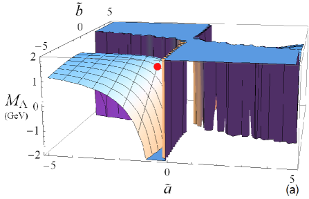
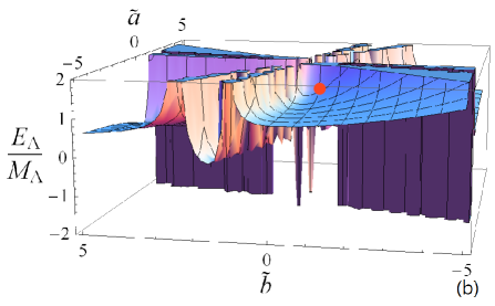
Figure 2: Sum-rule result in the $\{\tilde{a},\tilde{b}\}$ plane for (a) vacuum mass $M_{\Lambda}$, and for (b) the ratio of the in-medium quasi-$\Lambda$ state energy $E_{\Lambda}$ to $M_{\Lambda}$. The point denoted by the red filled circle corresponds to the result obtained with the Ioffe’s choice for the interpolating fields (31). Borel mass is set at $M^{2}=1.1~{}\textrm{GeV}^{2}$.

First of all, the two free parameters $\tilde{a}$ and $\tilde{b}$ in the generalized $\Lambda$ interpolating fields (27) should be confined before calculating the physical properties of the ground resonance. In Fig. 2, one can find $\tilde{a}$ and $\tilde{b}$ dependence of the vacuum mass $M_{\Lambda}$ and the ratio between the medium energy of the quasi-$\Lambda$ state $E_{\Lambda}$ to $M_{\Lambda}$. In principle, if one can obtain the complete OPE of the correlation function, the sum rules for the physical properties should not depend on the choice of $\tilde{a}$ and $\tilde{b}$. However, as we only have limited information for the condensates, the OPE have to be truncated at some finite order and subsequently, the sum rules can have singular and unstable region in the $\{\tilde{a},\tilde{b}\}$ plane. We assume that there is no physically important singularity that appears only for a specific linear combination of basis set (27) as the linear combination corresponds to just a linear superposition of possible spectral structures which commonly contain the same physical state. Hence, small fluctuation in the coefficient space $\{\tilde{a},\tilde{b}\}$ is possible and a reliable sum rules should not drastically change by such a small fluctuation. As can be found in Fig. 2(a), the sum rule for vacuum mass becomes unstable at $|\tilde{a}|\leq 1$ region so that the sum rule with Ioffe’s choice (31) lies on the boundary of stable region, which means that the calculated property can drastically change by small variations in $\{\tilde{a},\tilde{b}\}$. Within the same choice (31), the ratio $E_{\Lambda}/M_{\Lambda}$ also lies on the unstable region and the value becomes $\sim 1.5$, which means that the quasi-$\Lambda$ state feels a strong repulsive potential [Fig. 2(b)]. The energy can be made less repulsive by including the following additional derivative expansion on spin-1 four-quark condensate:

$$\langle\bar{s}\gamma_{\mu}s\bar{q}q\rangle_{\rho,I} \Rightarrow x^{\nu}\langle\bar{s}\gamma_{\mu}D_{\nu}s\bar{q}q\rangle_{\rho,I},$$ (62)

$$\langle\bar{s}\gamma_{\mu}iD_{\nu}s\bar{q}q\rangle_{\rho,I} =\frac{1}{4}g_{\mu\nu}m_{s}\langle\bar{s}s\bar{q}q\rangle_{\rho,I}+\frac{4}{3}\left(u_{\mu}u_{\nu}-\frac{1}{4}g_{\mu\nu}\right)\left(\langle s^{\dagger}iD_{0}s\bar{q}q\rangle_{\rho,I}-\frac{1}{4}m_{s}\langle\bar{s}s\bar{q}q\rangle_{\rho,I}\right),$$ (63)

where we used factorization (40) for both the trace and symmetric traceless parts. By adopting these additional steps and condensates such as $\langle q^{\dagger}iD_{0}q\rangle_{\rho,I}$, one can obtain a result similar to that of Ref. Jin:1993fr . However, such derivative expansion and factorization may cause large uncertainty and constitutes only part of the higher dimensional contributions. Moreover, even if these artificial steps are considered, with parameter set of $y\simeq 0.1$, $f_{1}\ll 1$, and $f_{2}\simeq 1$, the quasi-$\Lambda$ state is still repulsive, not consisted with the light-bounded state observed from the $\Lambda$ hyper-nuclei experiments Millener:1988hp .

Therefore $\tilde{a}$ and $\tilde{b}$ should be redefined to ensure small variation of sum rules in the “small perturbation” in $\{\tilde{a},\tilde{b}\}$ plane. As one can find in Fig. 2(b), the quasi-$\Lambda$ pole becomes stable and bounded in large $|\tilde{a}|$. This tendency can be clearly found from the cross-sections in Fig. 2 for a fixed $\tilde{a}$ given in Fig. 3.

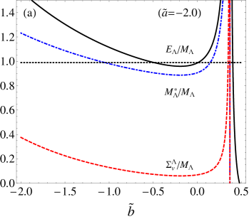
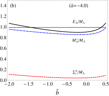
Figure 3: Ratios of the in-medium quasi-$\Lambda$ state energy, scalar, and vector self energies to its vacuum mass for $\tilde{a}=$ -2.0 (left) and -4.0 (right) as a function of $\tilde{b}$. Black dotted line represents 0.99.

The stable range of $\tilde{b}$ for the quasi-$\Lambda$ pole appears from $\tilde{a}\sim-2$ but the range is still narrow [Fig. 3(a)]. In the region where $|\tilde{a}|$ is large [Fig. 3(b)], one finds that the stable range of $\tilde{b}$ becomes wider. The stable range of $\tilde{b}$ can be identified as $-0.5<\tilde{b}<0$ at $|\tilde{a}|\gg 2$. We sampled the 9 stable points in $\{\tilde{a},\tilde{b}\}$ plane and averaged the sum rules from these points:

$$\{(\tilde{a},\tilde{b})\}=\big{\{} (-1.80,-0.10),(-1.80,-0.15),(-1.80,-0.20),$$

$$(-2.00,-0.05),(-2.00,-0.15),(-2.00,-0.25),$$

$$(-2.20,-0.00),(-2.20,-0.15),(-2.20,-0.30)\big{\}},$$ (64)

where the central point is $\{-2.00,-0.15\}$. If one takes the factorization constant $k_{1}$ less than 1, the central point of the stable region should be located at $\tilde{a}<-2$.

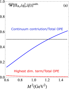
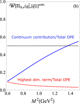
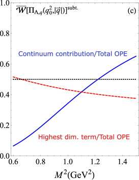
Figure 4: Ratios of the Borel-transformed-continuum contribution and highest-dimensional condensate terms to the Borel transformed subtracted total OPE of the $\Lambda$ for the three different invariants (a) $\Pi_{\Lambda,s}$, (b) $\Pi_{\Lambda,u}$, and (c) $\Pi_{\Lambda,q}$. The black dotted line represents 50%.

The next task is identifying a reliable range of the Borel mass. Again, if one could obtain “the complete OPE” of each invariant, the physical observable should not depend on Borel mass. However, as the OPE is truncated, the reliable sum rules should be found through the specific range of Borel mass called the Borel window. We used the following simple criteria: (i) the continuum contribution should not exceed 50% of the total OPE contribution and (ii) the highest mass dimensional condensate terms should not exceed 50% of the total OPE contribution. If the OPE of each invariant is a well constructed asymptotic series, the sum rules should show “plateau” or at least very weak dependence in the Borel mass. In Fig. 4, one can find that the Borel window can be set as $1.0~{}\textrm{GeV}^{2}\leq M^{2}\leq 1.2~{}\textrm{GeV}^{2}$. As can be found in the latter part, the sum rules are almost independent on Borel mass in this window.

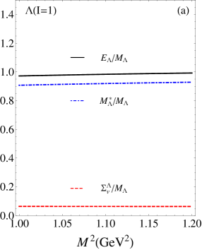
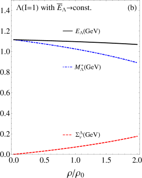
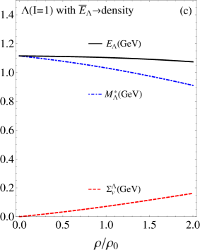
Figure 5: (a) Ratios and (b), (c) sum rules for the quasi-$\Lambda$ self-energies and the quasi-$\Lambda$ pole. $\rho=\rho_{0}$ in graph (a). In the linear density approximation, in-medium $\Lambda$ sum rules do not depend on iso-spin asymmetry of the surrounding matter. Graph (b) has been plotted with constant quasi-anti $\Lambda$ pole and graph (c) has been plotted with density dependent quasi-anti $\Lambda$ pole. Units for the graphs in (b) and (c) are GeV.

The sum-rule results for the quasi-$\Lambda$ state have been plotted in Fig. 5. The scalar attraction has been found as $M^{*}_{\Lambda}/M_{\Lambda}\simeq 85\%$ and the vector repulsion as $\Sigma^{\Lambda}_{v}/M_{\Lambda}\leq 10\%$ [Fig. 5(a)]. Comparing with the results Jin:1993fr where Ioffe’s choice has been used, our results show much weaker strength of attraction and repulsion. Comparing the strength of the self-energies with the self-energies of the nucleon sum rules Drukarev:1988kd ; Cohen:1991js ; Furnstahl:1992pi ; Jin:1992id ; Jin:1993up ; Cohen:1994wm ; Jeong:2012pa , one can find the ratio as $\Sigma_{s,\Lambda}/\Sigma_{s,N}\simeq 0.31$ and $\Sigma_{v,\Lambda}/\Sigma_{v,N}\simeq 0.26$, almost $30\%$ of the nucleon case. It means that the naive valence quark number counting may not be good for the determination of interaction strength between nucleon and hyperon. The net effect, estimated from the ratio $E_{\Lambda}/M_{\Lambda}$, is an attraction in the nuclear matter within 10 MeV scale. As the spin-orbit coupling in $\Lambda$ hyper-nuclei is expected to be weak Brockmann:1977es ; Hiyama:2000jd , the mean-field type phenomenology should explain the experimental observation of weakly bounded quasistate, which is now well reproduced in the sum-rule approach.

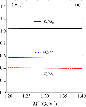
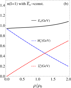
Figure 6: (a) Ratios and (b), (c) sum rules for neutron self-energies and the quasineutron pole in the neutron matter [$\rho=\rho_{0}$ in graph (a)]. Graph (b) has been plotted with constant quasi-antineutron pole and graph (c) has been plotted with density dependent quasi-antineutron pole. Units for the graphs in (b) and (c) are GeV.

As discussed in detail in Appendix A, we will consider the most general form for the twist-4 matrix elements in this work allowing for matrix elements not considered previously in Ref. Jeong:2012pa . Hence, the nucleon sum rules should be reexamined. The nucleon sum rules in the iso-spin-symmetric condition ($I=0$) do not show significant difference from the results of Ref. Jeong:2012pa . For the neutron matter ($I=1$) case, each sum rule for neutron and $\Sigma^{+}$ with renewed four-quark OPE and twist-4 matrix elements is plotted in Figs. 6 and 7, respectively. The quasi-neutron pole is slightly repulsive with the scalar attraction $M^{*}_{n}/M_{n}\simeq 55\%$ and the vector repulsion $\Sigma^{n}_{v}/M_{n}\simeq 40\%$ [Fig. 6(a)]. If one regards the quasi-antipole as a given constant, the quasineutron pole monotonically increases but if the pole has the density dependence, it decreases after $\rho/\rho_{0}\sim 0.6$ [Figs. 6(b) and 6(c)]. This density behavior is only reliable near $\rho/\rho_{0}\sim 1$; $0.5<\rho/\rho_{0}<1.5$.

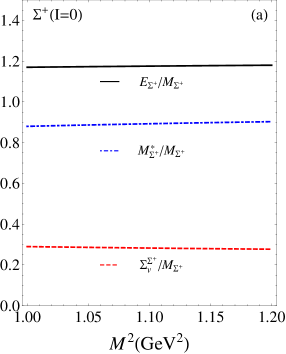
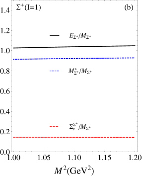
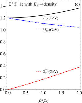
Figure 7: (a), (b) Ratios and (c) sum rules for $\Sigma^{+}$ self-energies and the quasi-$\Sigma^{+}$ pole. Graph (a) is plotted in iso-spin-symmetric condition ($I=0$, $\rho=\rho_{0}$) and graph (b) is plotted in neutron matter condition ($I=1$, $\rho=\rho_{0}$). For the in-medium $\Sigma^{+}$ sum rules, it is negligible for the difference between the constant and density-dependent quasi-anti $\Sigma^{+}$ pole case. Units for the graph in panel (c) are GeV.

Among the $\Sigma$ family, we have calculated the in-medium $\Sigma^{+}$ sum rules as it is expected to have lowest quasiparticle energy in the neutron matter when the electromagnetic interaction is neglected. As one can find in Fig. 7, sum rules show a weak scalar attraction $M^{*}_{\Sigma^{+}}/M_{\Sigma^{+}}\simeq 90\%$, a strong vector repulsion $\Sigma^{\Sigma^{+}}_{v}/M_{\Sigma^{+}}\simeq 30\%$ and a strong net repulsion $E_{\Sigma^{+}}/M_{\Sigma^{+}}\simeq 120\%$ in the iso-spin-symmetric ($I=0$) condition. Then the total repulsion exists in the order of 100 MeV scale, which fits with the experimental observation from $\Sigma$ hyper-nuclei Noumi:2001tx . In the neutron matter condition ($I=1$), the vector repulsion becomes weaker $\Sigma^{\Sigma^{+}}_{v}/M_{\Sigma^{+}}\simeq 15\%$ and the net repulsive effect reduces $E_{\Sigma^{+}}/M_{\Sigma^{+}}\simeq 105\%$. Although the repulsion becomes weaker in the neutron matter, the quasi-$\Sigma^{+}$ energy monotonically increases [Fig. 7(c)] and it never crosses with the quasineutron energy at least in the region $0.5<\rho/\rho_{0}<1.5$.

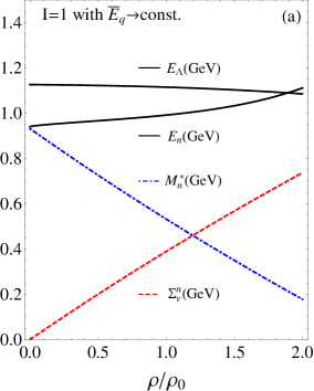
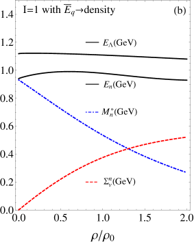
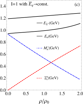
Figure 8: Comparison of the density behavior between $\Lambda$, $\Sigma^{+}$ hyperon and neutron sum rules in the neutron matter. Only graph (a) where constant quasi-antipoles are assigned shows the cross of quasibaryon energy. Units are GeV.

To discuss whether hyperons appear in the nuclear matter, the density behavior of the quasibaryon states should be compared with each other. The density behavior is plotted in Fig. 8. In the plots, only the quasi-$\Lambda$ state has a possibility to be lower in energy than the quasineutron state in the neutron matter. In the case where the quasi-antipole is just a given constant, the quasi-$\Lambda$ pole crosses with the quasineutron pole at $\rho/\rho_{0}\simeq 1.8$. In the other cases, including the density behavior of $\Sigma^{+}$, the crossing never occurs: the $\Sigma$ family ($I=1$) could be excluded in the discussion for early appearance of hyper-nuclear matter problem. Because our sum rules are only reliable near the normal density region $0.5<\rho/\rho_{0}<1.5$, we can conclude that the early crossing of the quasineutron and hyperon do not occur in the reliable region so that the onset of hyper-nuclear matter at low density becomes unlikely. To extend our result to the higher-density region, the density dependence for the condensates should be known beyond the linear density approximation.

V Discussion and Conclusions

Starting from the most general interpolating fields without derivatives for the nucleon, $\Sigma$ and $\Lambda$ hyperon as given in Sec. II, we obtained the optimal set in the parameter space for the interpolating fields that gives the most stable sum rules. The famous construction scheme known as Ioffe’s choice for interpolating fields would be suitable for the nucleon and the $\Sigma$ hyperon. However, for the $\Lambda$ hyperon, a different linear combination should be used to ensure the stability of the sum rules and subsequent results consistent with the experimental observation Millener:1988hp ; Noumi:2001tx . The basis with scalar diquark structure $u^{T}C\gamma_{5}d$ has to be emphasized for this purpose. Specifically, the “stabilized” interpolating fields for $\Lambda$ can be obtained by requiring $\tilde{a}\leq-2$ and $\tilde{b}\simeq-0.2$ in the general expression (27). In this renewed approach, the quasi-$\Lambda$ state is the light-bounded state described by a weak scalar attraction and vector repulsion. The strength of the self-energies is 30% of the self-energies calculated in the nucleon sum rules Cohen:1991js ; Furnstahl:1992pi ; Jin:1992id ; Jin:1993up ; Cohen:1994wm ; Jeong:2012pa . In the sum rules where the quasi-anti pole is given as a constant calculated at the saturation nuclear matter density, the quasi-$\Lambda$ energy crosses with the quasineutron energy at $\rho/\rho_{0}\simeq 1.8$. In the case where the quasi-antipole is calculated self consistently, the quasihyperon energy does not cross with the quasineutron energy. As the linear density approximation for the condensates is reliable only near the saturation density, the sum-rule predictions are expected to be valid near the saturation density region $0.5<\rho/\rho_{0}<1.5$. To extend the reliable results to the region $\rho/\rho_{0}>1.5$ the higher density dependence in the condensate should be known. Thus, one can claim that the onset of hyper-nuclear matter at low density would not occur at least up to the density region $\rho/\rho_{0}\leq 1.5$. The large portion of the scalar diquark structure $u^{T}C\gamma_{5}d$ in the interpolating field ensures the stability of the sum rules and the acceptable density behavior of the quasi-$\Lambda$ state. Hence, we expect that a good description of the $\Lambda$ can be obtained by introducing a scalar field $\phi^{\dagger}_{a}$ to describe the two light quarks as an single effective degree of freedom which contains the quantum number of $\epsilon_{abc}[u_{b}^{T}C\gamma_{5}d_{c}]$ ($s^{P}=0^{+}$, $I=0$) as has been pursued in Ref. Kim:2011ut .

The diquark structures of the interpolating fields for various baryons differ from each other. For the nucleon case with Ioffe’s choice (21), there is no unique way to make the diquark structure which consists of two light quarks. If the two quarks are combined in different flavor, scalar $u^{T}C\gamma_{5}d$ and pseudoscalar $u^{T}Cd$ structures are possible, but if the diquark is in the same flavor, it should have nonzero spin structure ($q^{T}C\gamma_{\mu}q$ or $q^{T}C\sigma_{\mu\nu}q$). Meanwhile, in the hyperon case, the diquark structure can be restricted by the choice of the interpolating fields and the sum-rules analysis. The diquark structure of Ioffe’s choice for $\Sigma$ hyperon (16) is the pseudovector $q_{1}^{T}C\gamma_{\mu}q_{2}$ where the light quark flavor $q_{1}$ and $q_{2}$ are in the $I=1$ configuration. The parity condition requires the light quarks in these diquarks to be in $l=1$ state in the nonrelativistic limit. As for the diquark structure $u^{T}C\gamma_{5}d$ in the stabilized $\Lambda$ interpolating field, the quarks will be in the relative angular momentum $l=0$ state in the nonrelativistic limit.

Our sum rules show that the quasi-$\Lambda$ state is slightly attractive and the quasi-$\Sigma$ state slightly repulsive in neutron matter. There seems to be a book keeping way of understanding the interaction of the quasihyperon with the medium in terms of the dominant diquark composed of light quarks. Namely, diquarks composed of lightquarks in the $l=0$ state are attractive while those in the $l=1$ state are repulsive. It would be interesting to investigate the validity of such a picture in models with explicit diquark fields Park:2016xrw , whose property change in nuclear medium can also be estimated in a constituent quark picture Park:2016xrw ; Park:2016cmg . Such topics will be pursed in a future work.

Appendix A Four-quark condensates

A.1 Twist-4 matrix elements from deep inelastic scattering experiment

Operator type	$\gamma-\gamma$	$\gamma_{5}\gamma-\gamma_{5}\gamma$	$\sigma-\sigma$
$t^{A}-t^{A}$	$\langle\bar{q}_{1}\gamma_{5}\gamma t^{A}q_{1}\bar{q}_{2}\gamma_{5}\gamma t^{A}q_{2}\rangle_{p,\textrm{s.t.}}\equiv T^{1}_{q_{1}q_{2}}$	$\langle\bar{q}_{1}\gamma t^{A}q_{1}\bar{q}_{2}\gamma t^{A}q_{2}\rangle_{p,\textrm{s.t.}}\equiv T^{2}_{q_{1}q_{2}}$	$\langle\bar{q}_{1}\sigma t^{A}q_{1}\bar{q}_{2}\sigma t^{A}q_{2}\rangle_{p,\textrm{s.t.}}\equiv T^{5}_{q_{1}q_{2}}$
$I-I$	$\langle\bar{q}_{1}\gamma_{5}\gamma q_{1}\bar{q}_{2}\gamma_{5}\gamma q_{2}\rangle_{p,\textrm{s.t.}}\equiv T^{3}_{q_{1}q_{2}}$	$\langle\bar{q}_{1}\gamma q_{1}\bar{q}_{2}\gamma q_{2}\rangle_{p,\textrm{s.t.}}\equiv T^{4}_{q_{1}q_{2}}$	$\langle\bar{q}_{1}\sigma q_{1}\bar{q}_{2}\sigma q_{2}\rangle_{p,\textrm{s.t.}}\equiv T^{6}_{q_{1}q_{2}}$

Table 1: Classification of the twist-4 operators and the corresponding matrix elements $T^{i}_{q_{1}q_{2}}$.

In this section, the discussion for the twist-4 matrix elements in Refs. Choi:1993cu ; Jeong:2012pa will be extended. Also, the consequence of this extension to sum-rule analysis will be presented. We start from the proton expectation value of the following generic twist-4 operators Choi:1993cu ; Jeong:2012pa :

$$\langle p|\bar{q}_{1}\Gamma^{\alpha}_{i}q_{1}\bar{q}_{2}\Gamma^{\beta}_{i}q_{2}|p\rangle_{\textrm{s.t.}}=\left(u^{\alpha}u^{\beta}-\frac{1}{4}g^{\alpha\beta}\right)\langle\bar{q}_{1}\Gamma_{i}q_{1}\bar{q}_{2}\Gamma_{i}q_{2}\rangle_{p,\textrm{s.t.}}=\left(u^{\alpha}u^{\beta}-\frac{1}{4}g^{\alpha\beta}\right)\frac{1}{4\pi\alpha_{s}}\frac{M_{n}}{2}T^{i}_{q_{1}q_{2}},$$ (65)

where $q_{1},q_{2}$ represents the quark flavor. In this study, the twist-4 operators which have strange quark flavor $\langle\bar{q}\Gamma_{i}q\bar{s}\Gamma_{i}s\rangle_{p,\textrm{s.t.}}$ are omitted because the assumed nuclear matter in $0.5<\rho/\rho_{0}<1.5$ will not allow for a larger external strange quark content. The operator type $\Gamma_{i}$ and the corresponding matrix elements $T^{i}_{q_{1}q_{2}}$ can be found in Table 1.

A.1.1 Twist-4 matrix elements for a single quark flavor

From the relation (84) of Ref. Jeong:2012pa and the “zero identity” presented in Refs. Thomas:2007gx ; Jeong:2012pa , the single quark flavored twist-4 operators whose matrix elements had been estimated from deep inelastic scattering (DIS) experiment Choi:1993cu ; Jeong:2012pa can be summarized as

$$[\bar{q}\gamma^{\alpha}t^{A}q\bar{q}\gamma^{\beta}t^{A}q]_{\textrm{s.t.}}= -\frac{5}{12}[\bar{q}\gamma^{\alpha}q\bar{q}\gamma^{\beta}q]_{\textrm{s.t.}}-\frac{1}{4}[\bar{q}\gamma_{5}\gamma^{\alpha}q\bar{q}\gamma_{5}\gamma^{\beta}q]_{\textrm{s.t.}}+\frac{1}{4}[\bar{q}\sigma_{\mu}^{~{}\alpha}q\bar{q}\sigma^{\mu\beta}q]_{\textrm{s.t.}},$$ (66)

$$[\bar{q}\gamma_{5}\gamma^{\alpha}t^{A}q\bar{q}\gamma_{5}\gamma^{\beta}t^{A}q]_{\textrm{s.t.}}= -\frac{5}{12}[\bar{q}\gamma_{5}\gamma^{\alpha}q\bar{q}\gamma_{5}\gamma^{\beta}q]_{\textrm{s.t.}}-\frac{1}{4}[\bar{q}\gamma^{\alpha}q\bar{q}\gamma^{\beta}q]_{\textrm{s.t.}}-\frac{1}{4}[\bar{q}\sigma_{\mu}^{~{}\alpha}u\bar{q}\sigma^{\mu\beta}q]_{\textrm{s.t.}}.$$ (67)

The matrix elements for the operators on the left-hand sides will be denoted $T^{1}_{qq}$ and $T^{2}_{qq}$ as given in Table 1. By using successive the Fierz rearrangement, the operator in $T^{5}_{qq}$ can be written as follows:

$$[\bar{q}\sigma_{\mu}^{~{}\alpha}t^{A}q\bar{q}\sigma^{\mu\beta}t^{A}q]_{\textrm{s,t}}= ~{}\frac{1}{2}[\bar{q}\gamma^{\alpha}q\bar{q}\gamma^{\beta}q]_{\textrm{s,t}}-\frac{1}{2}[\bar{q}\gamma_{5}\gamma^{\alpha}q\bar{q}\gamma_{5}\gamma^{\beta}q]_{\textrm{s,t}}-\frac{1}{6}[\bar{q}\sigma_{\mu}^{~{}\alpha}q\bar{q}\sigma^{\mu\beta}q]_{\textrm{s,t}},$$ (68)

which leads to the following relation:

$$\epsilon_{abc}\epsilon_{a^{\prime}b^{\prime}c}[\bar{q}_{a^{\prime}}\sigma q_{a}\bar{q}_{b^{\prime}}\sigma q_{b}]_{\textrm{s,t}}= ~{}\frac{2}{3}[\bar{q}\sigma_{\mu}^{~{}\alpha}q\bar{q}\sigma^{\mu\beta}q]_{\textrm{s.t.}}-2[\bar{q}\sigma_{\mu}^{~{}\alpha}t^{A}q\bar{q}\sigma^{\mu\beta}t^{A}q]_{\textrm{s.t.}}$$

$$= -[\bar{q}\gamma^{\alpha}q\bar{q}\gamma^{\beta}q]_{\textrm{s.t.}}+[\bar{q}\gamma_{5}\gamma^{\alpha}q\bar{q}\gamma_{5}\gamma^{\beta}q]_{\textrm{s.t.}}+[\bar{q}\sigma_{\mu}^{~{}\alpha}q\bar{q}\sigma^{\mu\beta}q]_{\textrm{s.t.}}.$$ (69)

The corresponding matrix elements can be expressed as

$$\langle\bar{q}\sigma q\bar{q}\sigma q\rangle_{\textrm{s,t}}= ~{}\frac{1}{4\pi\alpha_{s}}\frac{M_{n}}{2}\bigg{[}-\frac{1}{2}([T^{4}_{uu}+T^{4}_{dd}]\mp[T^{4}_{uu}-T^{4}_{dd}]I)+\frac{1}{2}([T^{3}_{uu}+T^{3}_{dd}]\mp[T^{3}_{uu}-T^{3}_{dd}]I)$$

$$\qquad\qquad\quad+\frac{1}{2}([T^{6}_{uu}+T^{6}_{dd}]\mp[T^{6}_{uu}-T^{6}_{dd}]I)\bigg{]}\rho,$$ (70)

where “$+$” and “$-$” stand for $u$ and $d$ quark flavor, respectively. In our previous work Jeong:2012pa , the matrix elements for the operator $\epsilon_{abc}\epsilon_{a^{\prime}b^{\prime}c}[\bar{q}_{a^{\prime}}\sigma q_{a}\bar{q}_{b^{\prime}}\sigma q_{b}]_{\textrm{s,t}}$ were neglected because the contribution of these operators to the DIS process was expected to be minimal in Ref. Jaffe:1981sz . However, as one can find in Eq. (70), in the case where $T^{3}_{qq}\neq 0$ and $T^{4}_{qq}\neq 0$, the matrix elements of $\langle\bar{q}\sigma q\bar{q}\sigma q\rangle_{\textrm{s,t}}$ cannot automatically be zero. In this study, we take the matrix elements $T^{6}_{qq}$ as free parameters and estimate their value. One needs additional assumption for the ratio $T^{6}_{uu}/T^{6}_{dd}$. As for $T^{1}_{qq}$ and $T^{2}_{qq}$, the ratios between $u$ and $d$ flavors can be assumed to be $T^{1}_{uu}/T^{1}_{dd}=T^{2}_{uu}/T^{2}_{dd}\simeq 6$ Jeong:2012pa from estimates of DIS experiment. Based on this observation, we will also take the ratio of $T^{6}_{uu}/T^{6}_{dd}\Rightarrow 6$. Then, $T^{3}_{qq}$ and $T^{4}_{qq}$ can be summarized as follows:

$$T^{3}_{qq}=-\frac{15}{4}T^{1}_{qq}+\frac{9}{4}T^{2}_{qq}-\frac{3}{2}T^{6}_{qq},$$ (71)

$$T^{4}_{qq}=-\frac{15}{4}T^{2}_{qq}+\frac{9}{4}T^{1}_{qq}+\frac{3}{2}T^{6}_{qq}.$$ (72)

The single quark flavored matrix elements are listed in Table 2.

$T^{1}_{uu}$	$T^{1}_{dd}$	$T^{2}_{uu}$	$T^{2}_{dd}$	$T^{3}_{uu}$	$T^{3}_{dd}$	$T^{4}_{uu}$	$T^{4}_{dd}$
$-0.071$	$-0.012$	$0.070$	$0.012$	$0.424-\frac{3}{2}T^{6}_{uu}$	$0.072-\frac{3}{2}T^{6}_{dd}$	$-0.424+\frac{3}{2}T^{6}_{uu}$	$-0.072+\frac{3}{2}T^{6}_{dd}$

Table 2: Table for the twist-4 matrix elements for a single quark flavor $T^{i}_{qq}$. Units are $\textrm{GeV}^{2}$.

A.1.2 Twist-4 matrix elements for mixed quark flavor

The matrix element $T^{1}_{ud}=-0.042~{}\textrm{GeV}^{2}$ had been uniquely determined by DIS experiment Choi:1993cu . Using the arguments in Refs. Choi:1993cu ; Jeong:2012pa , $T^{2}_{ud}=0.041~{}\textrm{GeV}^{2}$ has also been estimated. For $T^{1}_{uu}$ and $T^{1}_{dd}$, one observes the relation $T^{1}_{ud}\simeq(T^{1}_{uu}+T^{1}_{dd})/2=-0.042~{}\textrm{GeV}^{2}$. Similarly, $T^{2}_{ud}\simeq(T^{2}_{uu}+T^{2}_{dd})/2=0.041~{}\textrm{GeV}^{2}$. Based on this observation, we claim that the other matrix elements also satisfy the same relation: $T^{3}_{ud}\simeq(T^{3}_{uu}+T^{3}_{dd})/2$ and $T^{4}_{ud}\simeq(T^{4}_{uu}+T^{4}_{dd})/2$. Then, for the mixed quark flavored case, the relation (70) can be rewritten as follows:

$$\langle\bar{u}\sigma u\bar{d}\sigma d\rangle_{\textrm{s.t.}}=~{}\frac{1}{4\pi\alpha_{s}}\frac{M_{n}}{2}\left(-T^{4}_{ud}+T^{3}_{ud}+\frac{7}{12}T^{6}_{uu}\right)\rho,$$ (73)

where the iso-spin-dependent pieces have been excluded by assumed symmetries. The mixed quark flavored matrix elements are listed in Table 3.

$T^{1}_{ud}$	$T^{2}_{ud}$	$T^{3}_{ud}$	$T^{4}_{ud}$
$-0.042$	$0.041$	$T^{3}_{ud}\simeq 0.250-\frac{3}{2}T^{6}_{ud}$	$T^{4}_{ud}\simeq-0.250+\frac{3}{2}T^{6}_{ud}$

Table 3: Table for the twist-4 matrix elements for mixed quark flavor $T^{i}_{ud}$. $T^{6}_{ud}=(7/12)T^{6}_{uu}$. Units are $\textrm{GeV}^{2}$.

A.2 Parameter dependence of the sum rule analysis

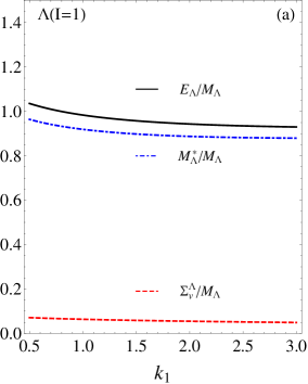
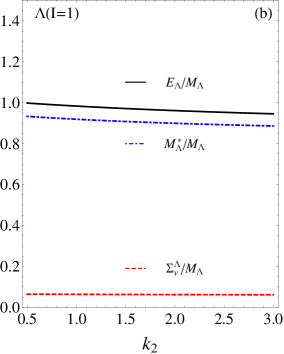
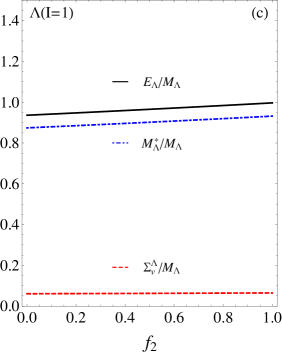
Figure 9: Factorization parameter dependence of the sum rule for the quasi-$\Lambda$ state ($\rho=\rho_{0}$, $M^{2}=1.1~{}\textrm{GeV}^{2}$). (a) $k_{1}$ dependence from the factorization $\langle\bar{q}q\bar{q}q\rangle_{\textrm{vac}}\Rightarrow k_{1}\langle\bar{q}q\rangle^{2}_{\textrm{vac}}$. (b) $k_{2}$ dependence from the factorization $\langle\bar{q}q\bar{s}s\rangle_{\textrm{vac}}\Rightarrow k_{2}\langle\bar{q}q\rangle_{\textrm{vac}}\langle\bar{s}s\rangle_{\textrm{vac}}$. (c) $f_{2}$ dependence from the factorization $\langle\bar{q}q\bar{s}s\rangle_{\textrm{med.}}\Rightarrow f_{2}\left(\langle\bar{s}s\rangle_{p}\langle\bar{q}q\rangle_{\textrm{vac}}+\langle[\bar{q}q]_{0}\rangle_{p}\langle\bar{s}s\rangle_{\textrm{vac}}\right)\rho$.

First, we examine the factorization parameter dependence of the sum rules. In Fig. 9, the $k_{1}$, $k_{2}$, and $f_{2}$ dependence of the quasi-$\Lambda$ self-energies are plotted. As can be seen in Fig. 9, the dependencies on the parameters $k_{1}$, $k_{2}$, and $f_{2}$ are weak in the quasi-$\Lambda$ sum rules. Hence, we have chosen the parameters as used in the previously reported studies Shifman:1978bx ; Ioffe:1981kw ; Reinders:1984sr ; Drukarev:1988kd ; Cohen:1991js ; Hatsuda:1991ez ; Furnstahl:1992pi ; Jin:1992id ; Jin:1993up ; Cohen:1994wm ; Jeong:2012pa : $k_{1},k_{2},f_{2}=1$. While we chose $k_{1},k_{2}=1$, the sum-rule results do not change much even if the scalar four-quark condensates are taken to be $50\%\sim 300\%$ of the estimated value.

The influences of $T^{6}_{uu}$ are plotted in Fig. 10. As can be found in Fig. 10(a), the quasi-neutron energy has weak dependence on $T^{6}_{uu}$ but each self-energy has non-negligible dependence. The scalar (vector) self-energy becomes enhanced (reduced) as $T^{6}_{uu}$ grows whereas the quasi-$\Lambda$ sum rules are almost independent on $T^{6}_{uu}$ [Fig. 10(b)]. The stabilized sum rules with the interpolating fields require very small $\tilde{b}$, which multiplies the twist-4 condensates term in the OPE. Hence, the contribution of the twist-4 condensates is minimal regardless of the value of matrix elements parametrized by $T^{6}_{uu}$ because $\tilde{b}$ is small. In Fig. 10(c), the nuclear symmetry energy is parametrized by $T^{6}_{uu}$. The symmetry energy becomes reduced and the cancellation mechanism between the vector and scalar becomes weaker as $T^{6}_{uu}$ grows. We have chosen $T^{6}_{uu}=0.2~{}\textrm{GeV}^{2}$ to ensure moderate strength of the cancelation mechanism shown in Figs. 10(a) and 10(c).

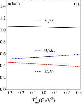
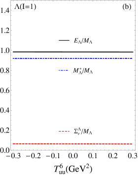
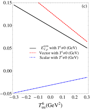
Figure 10: Sum rules with various $T^{6}_{uu}$ ($\rho=\rho_{0}$). (a) the quasineutron sum rules in the neutron matter. (b) the quasi-$\Lambda$ sum rules in the neutron matter. (c) nuclear symmetry energy. The OPE terms for the symmetry energy can be found in Ref. Jeong:2012pa . Units for graph (c) are GeV.

References

- (1) P. B. Demorest, T. Pennucci, S. M. Ransom, M. S. E. Roberts, and J. W. T. Hessels, Nature (London) 467, 1081 (2010).
- (2) J. Antoniadis et al., Science 340, 1233232 (2013).
- (3) E. S. Fraga, A. Kurkela and A. Vuorinen, Astrophys. J. 781, no. 2, L25 (2014) .
- (4) A. Drago, A. Lavagno, G. Pagliara and D. Pigato, Phys. Rev. C 90, no. 6, 065809 (2014) .
- (5) M. Drews and W. Weise, Phys. Rev. C 91, no. 3, 035802 (2015) .
- (6) N. K. Glendenning, Astrophys. J. 293, 470 (1985).
- (7) R. Knorren, M. Prakash and P. J. Ellis, Phys. Rev. C 52, 3470 (1995).
- (8) B. A. Li, L. W. Chen and C. M. Ko, Phys. Rept. 464, 113 (2008).
- (9) M. A. Shifman, A. I. Vainshtein and V. I. Zakharov, Nucl. Phys. B 147, 385 (1979); B 147 448 (1979); B 147 519 (1979).
- (10) B. L. Ioffe, Nucl. Phys. B 188, 317 (1981).
- (11) L. J. Reinders, H. Rubinstein and S. Yazaki, Phys. Rept. 127, 1 (1985).
- (12) E. G. Drukarev and E. M. Levin, Nucl. Phys. A 511, 679 (1990).
- (13) T. D. Cohen, R. J. Furnstahl and D. K. Griegel, Phys. Rev. Lett. 67, 961 (1991).
- (14) R. J. Furnstahl, D. K. Griegel and T. D. Cohen, Phys. Rev. C 46, 1507 (1992).
- (15) X. Jin, T. D. Cohen, R. J. Furnstahl and D. K. Griegel, Phys. Rev. C 47, 2882 (1993).
- (16) X. Jin, M. Nielsen, T. D. Cohen, R. J. Furnstahl and D. K. Griegel, Phys. Rev. C 49, 464 (1994).
- (17) T. D. Cohen, R. J. Furnstahl, D. K. Griegel and X. m. Jin, Prog. Part. Nucl. Phys. 35, 221 (1995).
- (18) T. Hatsuda and S. H. Lee, Phys. Rev. C 46, 34 (1992).
- (19) F. Klingl, N. Kaiser and W. Weise, Nucl. Phys. A 624, 527 (1997).
- (20) S. Leupold, W. Peters and U. Mosel, Nucl. Phys. A 628, 311 (1998).
- (21) F. Klingl, S. s. Kim, S. H. Lee, P. Morath and W. Weise, Phys. Rev. Lett. 82, 3396 (1999) Erratum: [Phys. Rev. Lett. 83, 4224 (1999)].
- (22) K. S. Jeong and S. H. Lee, Phys. Rev. C 87, no. 1, 015204 (2013).
- (23) J. M. Alarcon, L. S. Geng, J. Martin Camalich and J. A. Oller, Phys. Lett. B 730, 342 (2014).
- (24) X. L. Ren, L. S. Geng and J. Meng, Phys. Rev. D 91, no. 5, 051502 (2015).
- (25) S. Durr et al., Phys. Rev. Lett. 116, no. 17, 172001 (2016).
- (26) Y. B. Yang et al. [xQCD Collaboration], Phys. Rev. D 94, no. 5, 054503 (2016).
- (27) D. J. Millener, C. B. Dover and A. Gal, Phys. Rev. C 38, 2700 (1988).
- (28) H. Noumi et al., Phys. Rev. Lett. 89, 072301 (2002) Erratum: [Phys. Rev. Lett. 90, 049902 (2003)].
- (29) X. M. Jin and R. J. Furnstahl, Phys. Rev. C 49, 1190 (1994).
- (30) X. M. Jin and M. Nielsen, Phys. Rev. C 51, 347 (1995).
- (31) T. D. Cohen, R. J. Furnstahl and D. K. Griegel, Phys. Rev. C 45, 1881 (1992).
- (32) S. Choi, T. Hatsuda, Y. Koike and S. H. Lee, Phys. Lett. B 312, 351 (1993).
- (33) R. Brockmann and W. Weise, Phys. Lett. B 69, 167 (1977).
- (34) E. Hiyama, M. Kamimura, T. Motoba, T. Yamada and Y. Yamamoto, Phys. Rev. Lett. 85, 270 (2000).
- (35) R. Thomas, T. Hilger and B. Kampfer, Nucl. Phys. A 795, 19 (2007).
- (36) K. Kim, D. Jido and S. H. Lee, Phys. Rev. C 84, 025204 (2011).
- (37) A. Park, P. Gubler, M. Harada, S. H. Lee, C. Nonaka and W. Park, Phys. Rev. D 93, no. 5, 054035 (2016).
- (38) W. Park, A. Park and S. H. Lee, Phys. Rev. D 93, no. 7, 074007 (2016).
- (39) R. L. Jaffe and M. Soldate, AIP Conf. Proc. 74, 60 (1981).
- (40) M. Beneke and V. M. Braun, Nucl. Phys. B 426, 301 (1994).
- (41) M. Beneke, Phys. Lett. B 344, 341 (1995).
- (42) A. Gomez Nicola, J. R. Pelaez and J. Ruiz de Elvira, Phys. Rev. D 82, 074012 (2010).
- (43) E. G. Drukarev, M. G. Ryskin and V. A. Sadovnikova, Phys. Rev. C 86, 035201 (2012).