Precise Determination of Charge Dependent Pion-Nucleon-Nucleon Coupling Constants

Abstract

We undertake a covariance error analysis of the pion-nucleon-nucleon coupling constants from the Granada-2013 np and pp database comprising a total of 6720 scattering data below LAB energy of 350 MeV. Assuming a unique pion-nucleon coupling constant in the One Pion Exchange potential above a boundary radius $r_{c}=3{\rm fm}$ we obtain $f^{2}=0.0763(1)$. The effects of charge symmetry breaking on the ${}^{3}P_{0}$, ${}^{3}P_{1}$ and ${}^{3}P_{2}$ partial waves are analyzed and we find $f_{p}^{2}=0.0761(4)$, $f_{0}^{2}=0.0790(9)$ and $f_{c}^{2}=0.0772(6)$ with a strong anti-correlation between $f_{c}^{2}$ and $f_{0}^{2}$. We successfully test normality for the residuals of the fit. Potential tails in terms of different boundary radii as well as chiral Two-Pion-Exchange contributions as sources of systematic uncertainty are also investigated.

I Introduction

The meson exchange picture is a genuine quantum field theoretical feature which implies, in particular, that the strong force between protons and neutrons at long distances is dominated by the exchange of the lightest hadrons compatible with the conservation laws, namely neutral and charged pions. The strong force acting between nucleons at sufficiently large distances or impact parameters $\gtrsim 3{\rm fm}$ is solely due to one pion exchange (OPE) and was suggested by Yukawa 80 years ago Yukawa:1935xg . The verification of this mechanism not only provides a check of quantum field theory at the hadronic level but also a quantitative insight onto the determination of the forces which hold atomic nuclei pauli1948meson . While the mass of the pion may be determined directly from analysis of their tracks or electroweak decays, the determination of the coupling constant to nucleons needs further theoretical elaboration. The pion-nucleon-nucleon coupling constant is rigorously defined as the $\pi NN$ vertex function when all three particles are on the mass shell and in principle any process involving the elementary vertices $p\to\pi^{0}p$, $n\to\pi^{0}n$, $p\to\pi^{+}n$ and $n\to\pi^{-}p$ (or their charge conjugated) is suitable for the determination of the corresponding couplings provided all other relevant effects are accounted for with an acceptable level of precision. In this work we extract these coupling constants from NN scattering data and look for signals of charge symmetry breaking.

The combinations entering in NN scattering are (we use the conventions of Dumbrajs:1983jd and when possible, for simplicity, omit the $\pi$ label),

$$f_{p}^{2} = f_{\pi^{0}pp}f_{\pi^{0}pp}$$ (1)

$$f_{0}^{2} = -f_{\pi^{0}nn}f_{\pi^{0}pp}$$ (2)

$$2f_{c}^{2} = f_{\pi^{-}pn}f_{\pi^{+}np}$$ (3)

Usually the charge symmetry breaking is restricted to mass differences by setting $f_{p}=-f_{n}=f_{c}=f_{0}=f$. The relevant relationship between the pseudo-scalar pion coupling constant, $g_{\pi NN}$, and the pseudo-vector one, $f_{\pi NN}$, is given by

$$\frac{g^{2}_{\pi^{a}NN^{\prime}}}{4\pi}=\left(\frac{M_{N}+M_{N^{\prime}}}{m_{\pi^{\pm}}}\right)^{2}f^{2}_{\pi^{a}NN^{\prime}}$$ (4)

where $N,N^{\prime}=n,p$ and $\pi^{a}=\pi^{0},\pi^{\pm}$ (the factor $m_{\pi^{\pm}}$ is conventional). Thus, we may define $g_{0}^{2}$, $g_{c}^{2}$ and $g_{p}^{2}$. We take $M_{p}=938.27231$ MeV the proton mass, $M_{n}=939.56563$ MeV the neutron mass, and $m_{\pi^{\pm}}=139.5675$ MeV the mass of the charged pion.

There is a long history of determinations of pion-nucleon coupling constants using different approaches. A variety of methods and reactions have been used since the seminal Yukawa paper. A more complete account of the subsequent numerous determinations can be traced from comprehensive overviews deSwart:1997ep ; Sainio:1999ba ; Bugg:2004cm . Here we will mainly review determinations based on NN-scattering.

The very first determination was made in 1940 by Bethe by looking at deuteron properties PhysRev.57.260 ; Bethe:1940zz soon after Yukawa proposed his theory and before the pion was experimentally discovered, finding the common value $f^{2}=0.077-0.080$. On a more theoretical ground, based on dispersion relations and the Partial Conservation of the Axial Current (PCAC) Goldberger and Treiman deduced a relation between the $\pi NN$ form factor, $G_{\pi NN}(t)$, the nucleon axial coupling constant, $g_{A}=1.26$, and the pion weak decay constant, $F_{\pi}=93.4(3)$ MeV. The relation, $G_{\pi NN}(0)F_{\pi}=M_{N}g_{A}$ Goldberger:1958tr , shown by Nambu to follow from chiral symmetry Nambu:1960xd , is strictly valid at the pion off-shell point, $q^{2}=0$, and numerically it yields $f_{\pi NN}^{2}=g_{A}^{2}m_{\pi^{+}}^{2}/(16\pi F_{\pi}^{2})=0.072$. Almost simultaneously, Chew proposed Chew:1958zz to determine it from the occurrence of the pion pole in the renormalized Born approximation, by using an extrapolation method which was implemented soon thereafter for np Cziffra:1959zza and pp MacGregor:1959zz data. The first direct and quantitative evidence for OPE was found in 1960 by Signell Signell:1960zz by fitting the neutral pion mass to the differential cross section in p-p scattering data. The method of partial wave analysis (PWA) was soon afterwards used by Macgregor et al. macgregor1964determination .

During many years $\pi N$ scattering determination through fixed-t dispersion relations was advocated as a precision tool, yielding initially $f_{c}^{2}=0.0790(10)$ Bugg:1973rv , and later providing $f_{c}^{2}=0.0735(15)$ Arndt:1990cn (see also Arndt:1994bu and references therein). The latest most accurate $\pi N$ scattering determinations are: i) the one based on the GMO rule Ericson:2000md , $g_{c}^{2}/(4\pi)=14.11(20)$ ($f_{c}^{2}=0.0783(11)$); ii) the one using fixed-t dispersion relations, $g_{c}^{2}/(4\pi)=13.76(8)$ Arndt:2006bf ; iii) the most recent one Baru:2010xn ; Baru:2011bw , based on $\pi N$ scattering lengths, $\pi^{-}d$ scattering and the GMO sum rule, yielding $g_{c}^{2}/(4\pi)=13.69(12)(15)=13.69(19)$. Another source of information has been the $\bar{N}N$ system, as shown by the Nijmegen group Timmermans:1990tz , providing $f_{c}^{2}=0.0751(17)$.

The modern era of high-quality NN interactions initiated by the Nijmegen group Stoks:1993tb enabled to decrease the reduced $\chi^{2}/\nu$ from 2 to 1, thanks to the implementation of charge dependence (CD), vacuum polarization, relativistic corrections and magnetic moments interactions, and a suitable selection criterion for compatible data. Their analysis comprised a total of 4313 NN scattering data. This promoted the determination of the pion-nucleon coupling constant from np and pp scattering to a competitively accurate approach. The main advantage of an NN analysis as compared to the $\pi N$ analysis, which has so far been restricted to charged pions, is that one can determine both neutral and charged-pion coupling constants simultaneously, to search for isospin breaking effects. The three compatible values, $f_{p}^{2}=0.0751(6)$, $f_{0}^{2}=0.0752(8)$ and $f_{c}^{2}=0.0741(5)$, were determined from NN scattering data Klomp:1991vz . The originally recommended charge independent value $f^{2}=0.0749(4)$ Klomp:1991vz was revised Stoks:1992ja and confirmed in the 1997 review on the status of the pion-nucleon-nucleon coupling constant deSwart:1997ep ; this is the most accurate NN determination to date. There, it was suggested that a charge-independence breaking could be checked with more data and better statistics. The most recent determinations of the Nijmegen group have been given after the inclusion of charge-independent chiral two-pion exchange ($\chi$TPE) potential Kaiser:1997mw which depends on three additional chiral constants, $c_{1}$, $c_{3}$, $c_{4}$, which also appear in $\pi N$ scattering. A combined fit of $f_{p}^{2}$ and $c_{1,3,4}$ to pp scattering data, provides the value $f_{p}^{2}=0.0756(4)$ Rentmeester:1999vw , and a simultaneous fit to pp+np data of a common $f^{2}$ and $c_{1,3,4}$ Rentmeester:2003mf provides linear correlations between $f^{2}$ and $c_{1,2,3}$.

Most of the analyses determining the pion nucleon coupling constants involve heavy statistical analysis for a large body of experimental data, mostly $\chi^{2}-$fits, which are subjected to a number of a posteriori tests evans2004probability . The verification of these tests buttress a sensible analysis of uncertainties of theoretical models Dobaczewski:2014jga . To the time of their analysis, the Nijmegen group Bergervoet:1988zz ; Stoks:1992ja checked the statistical quality of pp fit residuals using the moments test, which for increasing orders over-weights the tails.

In this paper we study the possible differences among the pion-nucleon coupling constants by analyzing np and pp scattering data using the NN Granada-2013, $3\sigma$-self consistent database, designed and analyzed recently Perez:2013cza ; Perez:2013jpa ; Perez:2014yla ; Perez:2014kpa  . There, we have selected 6713 out of 8000 published np and pp experimental data for LAB energies below 350 MeV and measured in the period 1950-2013, which satisfactorily verify the tail-sensitive test Aldor2013 , based on the quantile-quantile plot for the combined np+pp residuals (see also Ref. Perez:2015pea for an application of these ideas to $\pi\pi$ scattering). As a side remark we note that the Uppsala controversial measurement Ericson:1995gr ; Rahm:1998jt , which gives the value $f^{2}=0.081$ and appears in Weinberg’s textbook Weinberg:1996kr , was disputed by the Nijmegen group Rentmeester:1998vf and contested Ericson:1998fq . An overview of the situation can be glanced in Blomgren:2000wq . This measurement has been rejected by our $3\sigma$ self-consistent database Perez:2013jpa . A latter re-measurement at IUCF by the partly the same group Sarsour:2004xx ; Sarsour:2006fd , which is compatible with the original Nijmegen PWA, is not rejected by the self-consistent $3\sigma$ criterion.

The paper is organized as follows. In Section II we describe the OPE potential, introduce our notation, and discuss the conditions under which we naturally expect to unveil charge dependence in the pion-nucleon coupling constants. In Section III we review the main aspects of our partial wave analysis and the Granada-2013 database. Our motivation for incorporating charge dependence in the P-waves, besides the customary charge dependence on S-waves implemented in all modern high quality fits, is presented in Section IV along with a discussion of our numerical results based on a covariance analysis. An effort to quantify systematic errors by analyzing the long range component of the CD-OPE is made in Section V. Finally, in Section VI conclusions are presented. In the Appendix we show the extended operator basis accommodating S-wave and P-wave charge dependence.

II Charge-Dependent One Pion Exchange

The charge-dependent, one-pion exchange (CD-OPE) potential incorporates charge symmetry breaking by considering the mass difference of the neutral and charged pions as well as assuming different coupling constants. We use the convention for $\pi NN$ Lagrangians defined in the review of ref. Dumbrajs:1983jd . The quantum mechanical potential which reproduces in Born approximation the corresponding Feynman diagrams for on-shell static nucleons, is given in the pp, nn and np channels as

$$V_{{\rm OPE},pp}(r) = f^{2}_{p}V_{m_{\pi^{0}},\rm OPE}(r),$$ (5)

$$V_{{\rm OPE},nn}(r) = f^{2}_{n}V_{m_{\pi^{0}},\rm OPE}(r),$$ (6)

$$V_{{\rm OPE},np}(r) = -f_{n}f_{p}V_{m_{\pi^{0}},\rm OPE}(r)-(-)^{T}2f^{2}_{c}V_{m_{\pi^{\pm}},\rm OPE}(r),$$ (7)

respectively. Here, $V_{m,\rm OPE}$ is given by

$$V_{m,\rm OPE}(r)=\left(\frac{m}{m_{\pi^{\pm}}}\right)^{2}\frac{1}{3}m\left[Y_{m}(r){\mathbf{\sigma}}_{1}\cdot\mathbf{\sigma}_{2}+T_{m}(r)S_{1,2}\right].$$ (8)

Here $Y_{m}$ and $T_{m}$ are the usual Yukawa functions,

$$Y(r) = \frac{e^{-mr}}{mr}$$ (9)

$$T(r) = \frac{e^{-mr}}{mr}\left[1+\frac{3}{mr}+\frac{3}{(mr)^{2}}\right],$$ (10)

$\sigma_{1}$ and $\sigma_{2}$ are the single nucleon Pauli matrices, and $S_{12}=3\sigma_{1}\cdot{\bf\hat{r}}\sigma_{2}\cdot{\bf\hat{r}}-\sigma_{1}\cdot\sigma_{2}$ is the tensor operator. Unfortunately, the CD-OPE potential by itself cannot be directly compared to experimental data, and the only way we know how to determine these pion-nucleon couplings is by carrying out a PWA.

From a purely classical viewpoint, in order to measure the nuclear force directly it would just be enough to hold and pull two nucleons apart at distances larger than their elementary size, which is or the order of $2{\rm fm}$ Perez:2013cza . For such an ideal experiment the behavior of the system at shorter distances would be largely irrelevant, because nucleons would behave as point-like particles. This situation would naturally occur if nucleons were truly infinitely heavy. In that case the potential would correspond to the static energy of a system with baryon number $B=2$ and total charge $Q=2,1,0$, for $pp$, $pn$ $nn$, respectively. Of course, the quantum mechanical nature of the nucleons prevents such a situation experimentally and we are left with scattering experiments. Good operating conditions are achieved when the maximum relative CM momentum, $p_{\rm max}$, is small enough to avoid complications due to inelastic channels and large enough to contain as many data as possible. This generates a resolution ambiguity of the order of the minimal relative de Broglie wavelength, $\lambda_{\rm min}=\Delta r\sim 1/p_{\rm max}$. Since the $NN\to\pi NN$ channel opens up at $p_{\rm max}\sim\sqrt{m_{\pi}M_{N}}\sim 360{\rm MeV}$, we have $\Delta r\sim 0.6{\rm fm}$. Unfortunately, in the quantum mechanical NN scattering problem the scales are somewhat intertwined, and thus some information on the unknown short-distance components of the potential have to be considered in order to evaluate the scattering amplitude, the cross section or the polarization asymmetry. The low energy behavior of the NN interaction is expected to depend strongly on its long distance properties. Although some coarse grained information of the unknown contribution is needed, it can be deduced from the experiment with an overall sufficient accuracy as to determine the differences between the pion-nucleon couplings. This viewpoint allows to determine a priori the number of independent parameters $N_{\rm Par}$ needed for a successful fit. These ideas where introduced by Aviles long ago Aviles:1973ee , and they underlie the recent NN analysis carried out by the present authors, where a large database, comprising about 8000 published experimental data measured in the period 1950-2013, was considered Perez:2013cza ; Perez:2013jpa .

II.1 The number of data

There is no symmetry reason why the strong force between protons and between neutrons should be exactly identical; if a difference exists one should be able to see it with a sufficiently large amount of experimental data. These differences are in fact small and hard to pin down because a priori the electromagnetic corrections should scale with the fine structure constant $\delta g/g\sim\alpha\sim 1/137$, and the strong (QCD) corrections should scale with the $u-d$ quark mass difference (relative to the $s$-quark mass) which means $\delta g/g\sim(m_{u}-m_{d})/\Lambda_{\rm QCD}\sim(M_{p}-M_{n})/\Lambda_{\rm QCD}\sim 1/100$, for $\Lambda_{\rm QCD}\sim 250{\rm MeV}$. This simple estimates suggest that in order to witness isospin violations in the couplings we should determine them with a target accuracy better than $1-2\%$, which is not too far from the most recent values. On a purely statistical basis the relative uncertainty due to $N$ independent measurements is $\Delta g/g\sim 1/\sqrt{N}$. If we have some extra parameters $(\lambda_{1},\dots,\lambda_{N_{\rm Par}})$,the condition $\Delta g\sim\delta g\sim 0.01-0.02$ would require $N=N_{\rm Dat}-N_{\rm Par}\sim 7000-10000$ independent degrees of freedom. Since $N_{\rm Dat}\gg N_{\rm Par}$ this is comparable to the total amount of existing elastic np and pp scattering data. While these are rough estimates, we stress the independence character of the measurements in order to make these estimates credible; it is not just a question of having more data. From the point of view of $\chi^{2}$-fits this requires passing satisfactorily normality tests guaranteeing the self-consistency of the fit. In particular, adding many incompatible data would invalidate this analysis.

II.2 Naturalness of fitting parameters

While our approach is based on a standard least squares optimization, which minimizes the distance between the theory and the experiment for many pp and np scattering data, it is important to mention that we do not consider that all fits are eligible and in fact some of them will be rejected. In what follows, we specify these criteria a priori.

As a matter of principle, we reject fits which display bound states in channels other than the deuteron (occurring in the ${}^{3}S_{1}-^{3}D_{1}$ channel only) which will be considered spurious. The appearance of such states in the fitting process is not so unlikely, particularly in the case of peripheral waves. This is usually detected by use of Levinson’s theorem, $\delta_{l}(0)-\delta_{l}(\infty)=n\pi$, which requires checking phases at energies much larger than the fitting range. An equivalent way to find spurious bound states is by checking the volume integrals (and high moments) for which a large degree of universality has been found Perez:2016vzj . Too large attractive couplings in the potential permitting a bound state would consequently generate unnaturally large volume integrals of the potentials.

In the case of the pion-nucleon coupling constant we expect some theoretical constraints to be fulfilled. The renowned Goldberger-Treiman relation was deduced as a consequence of exact PCAC, and yields the value (in the isospin limit)

$$G_{\pi NN}(0)=M_{N}g_{A}/F_{\pi}$$ (11)

The physical coupling constant corresponds to $g_{\pi NN}\equiv G_{\pi NN}(m_{\pi}^{2})>G_{\pi NN}(0)$. It is expected to be larger than value appearing in GT-relation. This suggests

$$g_{\pi NN}>M_{N}g_{A}/F_{\pi}$$ (12)

and hence, for the PDG values $F_{\pi^{+}}^{\rm PDG}=92.21(14){\rm MeV}$ and $g_{A}=1.2723(23)$,

$$f_{\pi NN}^{2}>f_{\pi NN,{\rm GT}}^{2}\equiv\frac{1}{16\pi}\left(\frac{g_{A}m_{\pi^{+}}}{F_{\pi}}\right)^{2}=0.07324(4)$$ (13)

The uncertainty is about $5\%$. More generally, a GT-discrepancy is defined (see e.g. Dominguez:1984ka for a review),

$$\Delta_{\rm GT}=1-\frac{M_{N}g_{A}}{g_{\pi NN}F_{\pi}}$$ (14)

The value of this number has been changing but typical values nowadays are at the few percent level, $\Delta_{\rm GT}\sim 0.01-0.03$. In the limit of zero quark masses, chiral symmetry becomes exact, and hence $\Delta_{\rm GT}={\cal O}(m_{\pi}^{2}/F_{\pi}^{2})$

The fact that $(m_{u}-m_{d})/(m_{u}+m_{d})\sim 1/3$ suggests that, if we obtain a GT discrepancy different from zero, about three more times precision would be needed to pin down isospin breaking. According to our $1/\sqrt{N_{\rm Dat}}$ estimate above, this can be accomplished by increasing the number of independent data by a factor of 10. At the level of isospin breaking some estimates have also been made Goity:1999by ; Goity:2002uh .

In the case of $\chi$TPE exchange, which will also be considered below, the chiral constants $c_{1,3,4}$ are saturated by meson exchange Bernard:1996gq . Actually, $c_{1}$ is saturated by scalar exchange. The saturation value is $c_{1}^{S}=-g_{S}c_{m}/m_{S}^{2}$. Taking $M_{N}=g_{S}F_{\pi}$ and $c_{m}=F_{\pi}/2$ , $m_{S}=m_{V}=F_{\pi}\sqrt{24\pi/N_{c}}$ Ledwig:2014cla and $M_{N}=N_{c}m_{\rho}/2$ we get $c_{1}^{S}\sim-N_{c}/(4\sqrt{2}m_{\rho})\sim-0.7{\rm GeV}^{-1}$. In the case of the constants $c_{3}$ and $c_{4}$, they are saturated by $\Delta$ resonance; taking $\Delta=M_{\Delta}-M_{N}$, the saturation values are $c_{2}^{\Delta}=-c_{3}^{\Delta}=2c_{4}^{\Delta}=g_{A}^{2}/(2\Delta)\sim 2.97{\rm GeV}^{-1}$. Of course, these are not very accurate values, but indicate the order of magnitude one should expect.

III The Granada-2013 analysis

In a series of works we have upgraded the NN database to include a total of 6720 np and pp published experimental data by using a coarse grained representation of the interaction, and applying stringent statistical tests on the residuals of the $\chi^{2}$-fits after implementing a $3\sigma$ self consistent selection process Perez:2014yla . The resulting Granada-2013 is at present the largest NN database which can be described by a CD-OPE contribution. There are about $60\%$ more data than the 4313 data used in the latest Nijmegen upgrade  deSwart:1997ep . This suggests that we can improve on the errors for the pion-nucleon couplings as discussed in the previous section.

We have discussed in detail the many issues in carrying out the data selection, the fit and the corresponding joint np+pp partial wave analysis. We review here the main aspects as a guideline and refer to those works for further details.

We separate the potential into two well defined regions depending on a chosen cut-off radius, $r_{c}$, fixed in such a way that for $r>r_{c}$ the CD-OPE is the only strong contribution. In addition, for $r>r_{c}$ we also include electromagnetic (Coulomb, vacuum polarization, magnetic moments) Perez:2013jpa and relativistic corrections which we simply add to the strong potential.

$$V({\bf r})=V_{\rm OPE}({\bf r})+V_{\rm EM}({\bf r}),\kern 28.45274ptr>r_{c}$$ (15)

Below the cut-off radius, $r<r_{c}$ we regard the NN force as unknown, and we use delta-shells located at equidistant points separated by $\Delta r=0.6{\rm fm}$, corresponding to the shortest de Broglie wavelength at pion production threshold. The fitting parameters are the real coefficients $(\lambda_{i})^{JS}_{ll^{\prime}}$ for each partial wave:

$$V_{l,l^{\prime}}^{JS}(r)=\frac{1}{2\mu}\sum_{i=1}^{N}(\lambda_{i})^{JS}_{ll^{\prime}}\delta(r-r_{i}),\kern 28.45274ptr\leq r_{c}.$$ (16)

where $\mu$ is the NN reduced mass. Alternatively the potential can be expanded in an operator basis extending the AV18 potentials in coordinate space, see appendix A. The transformation between partial wave and operator basis was given in Ref. Perez:2013jpa .

It turns out that $r_{c}=3{\rm fm}$ provides statistically satisfactory fits to the selected $3\sigma$-self consistent Granada-2013 database. While it would be interesting to separate explicitly the known from the unknown pieces of the interaction below the cut-off radius $r_{c}$, this is actually a complication in the fitting procedure, and will not change the values of the most-likely pion-nucleon coupling constants. Another advantage of taking $r_{c}=3{\rm fm}$ is that in our analysis there is no need of form factors of any kind, and thus we are relieved from disentangling finite size effects, quark exchange and the intrinsic resolution $\Delta r$ inherent to any finite energy PWA 

The possible $A_{y}$ problem for np scattering, raised by the data of Ref. Braun:2008eh , suggested a sizable isospin breaking of coupling constants. The problem was re-analyzed theoretically in ref. Gross:2008pd , and motivated the reanalysis of the data Weisel:2010zz and the disentanglement between systematic and statistical errors. Actually, in ref. Gross:2008pd it was found that these data might be explained in an isolated fashion when isospin was broken. Thus, we allow this isospin breaking to foresee the possibility of recovering the data.

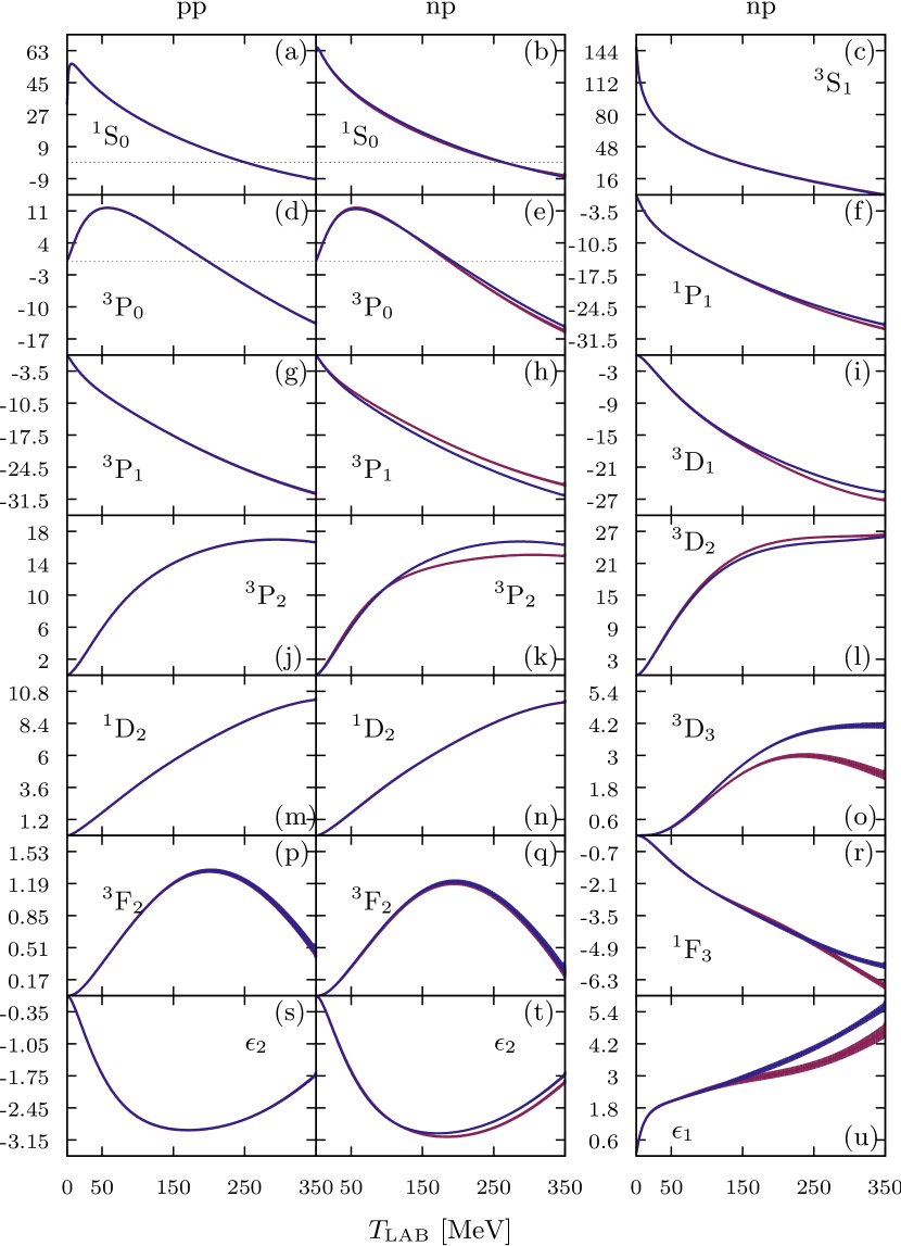
Figure 1: (Color online) Phaseshifts obtained from a partial waves analysis to pp and np data and statistical uncertainties. Blue band from Perez:2013jpa and red band from a fit with charge symmetry breaking on the ${}^{3}P_{0}$, ${}^{3}P_{1}$ and ${}^{3}P_{2}$ partial waves.

IV Statistical analysis

In our previous analysis we took a fixed common value for the pion-nucleon coupling constant suggested by the Nijmegen group. When we relax this assumption and also fit the pion-nucleon coupling constant as another parameter in the potential, we obtain $f^{2}=0.0763(1)$, which is $3\sigma$ compatible with the Nijmegen recommendation Klomp:1991vz , $f^{2}=0.0749(4)$ and more accurate.

IV.1 Charge symmetry breaking on $S$- and $P$ waves

An old problem in NN scattering fitting is if it is possible to predict the neutron-neutron potential fron np and pp data. A necessary condition would be that the unknown piece of the short distance interaction for np and pp coincide in the isovector channels. Once we allow to vary the coupling constants $f_{p}^{2}$, $f_{0}^{2}$ and $f_{c}^{2}$ from their common value $f^{2}$ we have first searched for a fit without CD in the $\lambda^{\prime}s$ (i.e. assuming that they are equal for np and pp). We get $\chi^{2}/\nu=1.2$ for CD-OPE above $r_{c}=3{\rm fm}$. On the other hand, $\chi^{2}/\nu=9$ for CD-OPE+$\chi$TPE above $r_{c}=1.8{\rm fm}$. Therefore, and in harmony with all high-quality previous attempts we cannot deduce nn-scattering below $r_{c}=3{\rm fm}$.

Following the common practice of other analyses Stoks:1993tb ; Wiringa:1994wb ; Machleidt:2000ge , we have previously allowed different pp and np parameters only on the ${}^{1}S_{0}$ partial wave Perez:2013cza ; Perez:2013oba ; Perez:2013jpa ; Perez:2013mwa and found that this symmetry breaking is indeed necessary to obtain an accurate description of the pp and np scattering data. The large collection of about $8000$ available data also makes it possible to test charge symmetry breaking on the parameterization of higher partial waves, e.g. ${}^{3}P_{0}$, ${}^{3}P_{1}$ and ${}^{3}P_{2}$.

To carry out such a test we have considered different np and pp parameters on those partial waves and performed a full PWA and selection process as described in Perez:2013mwa ; Perez:2013jpa , by fitting the delta-shell potential parameters to the complete database and then applying the $3\sigma$ rejection criterion iteratively until a self consistent database is obtained. The consistent database obtained in this case has $3006$ pp data and $3735$ np data, including normalizations, and the value for the chi square per number of data is $\chi^{2}/N_{\rm data}=1.02$. When comparing with our previous consistent data base Perez:2013jpa this symmetry breaking can only describe $21$ additional data out of more than $1000$ rejected data. Fig. 1 compares the low angular momentum phaseshifts of the PWA in Perez:2013jpa (blue bands) with this new analysis (red bands). The pp phaseshifts show no significant difference, while the np ones are statistically different and the differences are even greater for higher angular momentum partial waves. Tabulated values for the lower phase-shifts for selected LAB energies are provided in Appendix B.

Table 1: The pion-nucleon coupling constants $f_{p}^{2}$, $f_{0}^{2}$ and $f_{c}^{2}$ determined from different fits to the Granada-2013 database and their characteristics. We indicate the partial waves where charge dependence is allowed.

$f_{p}^{2}$	$f_{0}^{2}$	$f_{c}^{2}$	CD-waves	$\chi^{2}_{pp}$	$\chi^{2}_{np}$	$\chi^{2}$	$N_{\rm Dat}$	$N_{\rm Par}$	$\chi^{2}/\nu$
0.075	idem	idem	${}^{1}S_{0}$	2997.29	3957.57	6954.86	6720	46	1.042
0.0763(1)	idem	idem	${}^{1}S_{0}$	2995.20	3952.85	6947.05	6720	47	1.041
0.0764(4)	0.0779(8)	0.0758(4)	${}^{1}S_{0}$	2994.41	3950.42	6944.83	6720	49	1.041
0.0761(4)	0.0790(9)	0.0772(5)	${}^{1}S_{0}$, $P$	2979.37	3876.13	6855.50	6741	55	1.025

Usually the charge symmetry breaking is restricted to mass differences by setting $f_{p}=-f_{n}=f_{c}=f$. The value $f^{2}=0.075$ recommended by the Nijmegen group Klomp:1991vz has been used in most of the potentials since the seminal 1993 partial wave analysis Stoks:1993tb . Here we test this charge independence with the large body of data available today, by using $f_{p}$, $f_{0}$, and $f_{c}$ as extra fitting parameters along with the previous $46$ delta-shell parameters. We show our results in Table 1 depending on different strategies regarding isospin breaking: S-waves, S- and P-waves, and in the coupling constants. The working group summary of 1999 provides a recent compilation of coupling constants in a chronological display Sainio:1999ba . The most recent determination Baru:2010xn ; Baru:2011bw , based on $\pi N$ scattering lengths and $\pi^{-}d$ scattering, and in the GMO sum rule, yields $g_{c}^{2}/(4\pi)=13.69(12)(15)=13.69(20)$. From our full covariance matrix analysis we get $g_{p}^{2}/(4\pi)=13.774(75)$, $g_{0}^{2}/(4\pi)=14.30(16)$ and $g_{c}^{2}/(4\pi)=13.984(82)$. The last value is $2\sigma$ compatible with these determinations, but slightly more accurate.

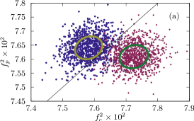
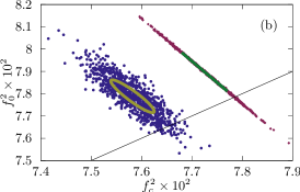
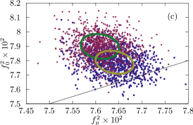
Figure 2: (Color Online) Correlation ellipses and scatter diagrams for the coupling constants $f_{c}^{2}$ , $f_{p}^{2}$ and $f_{0}^{2}$ appearing in the OPE potential from a PWA with (yellow line and blue dots) and without (green line and red diamonds) charge independence on the $P$ waves and a $3\sigma$ consistent database. The black diagonal line indicates $f_{c}^{2}=f_{p}^{2}=f_{0}^{2}$

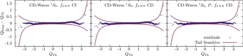
Figure 3: (Color Online) Rotated quantile-quantile plots for the fits introduced in this work. All points should be inside the confidence band to state that residuals of the fit follow a normal distribution $N(0,1)$, in which case the fit is self-consistent a posteriori. Left panel, assuming a charge independent pion-nucleon constant used as a fitting parameter and charge symmetry breaking only on the ${}^{1}S_{0}$ partial wave parameters. Central panel, assuming three different charge dependent pion-nucleon constants used as a fitting parameters and charge symmetry breaking only on the ${}^{1}S_{0}$ partial wave parameters. Right panel, assuming three different charge dependent pion-nucleon constants used as a fitting parameters and charge symmetry breaking on the ${}^{1}S_{0}$ and $P$ partial wave parameters

The fitting delta-shell parameters obtained in our different strategies, regarding charge independence breaking in just S-waves and charge independence breaking in S and P waves, can be seen in Tables 2 and 3 respectively. We use the resulting parameters along with their covariance matrix to calculate $f_{p}^{2}$, $f_{0}^{2}$ and $f^{2}_{c}$, and propagate the corresponding statistical uncertainties and test charge dependence. Fig. 2 shows the $1\sigma$ correlation ellipses along with the scatter diagram resulting from drawing $1000$ random variates following the multivariate normal distribution dictated by the covariance matrix. The fit without charge dependence on the $P$ waves is indicated by the blue dots and yellow line while the fit with charge dependence on the $P$ waves corresponds to the red diamonds and green line. Charge independence, $f_{p}^{2}=f_{0}^{2}=f_{c}^{2}$, is marked by the diagonal black line. Several aspects should be noted from Fig. 2. First, while the values on Table 1 seem to suggest that the determinations with and without charge charge dependent $P$ waves for $f_{0}^{2}$ and $f_{c}^{2}$ are $1$ and $2\sigma$ compatible respectively, in fact the strong anti-correlation between the two coupling constants makes the determinations completely incompatible. The determination with charge dependence on the $S$ waves only is compatible with the $f_{p}^{2}=f_{0}^{2}=f_{c}^{2}=0.0763(1)$ fit at the two sigma level; this is in accordance with the slight decrease in $\chi^{2}$ in spite of the fact that two extra parameters are fitted. Finally, the fit with charge dependent $P$ waves is incompatible with $f_{p}^{2}=f_{0}^{2}=f_{c}^{2}$, once again due to the strong anti-correlation between $f_{0}^{2}$ and $f_{c}^{2}$.

Table 2: Fitting delta-shell parameters $(\lambda_{n})^{JS}_{l,l^{\prime}}$ (in ${\rm fm}^{-1}$) with their errors for all states in the $JS$ channel for a fit with isospin symmetry breaking on the ${}^{1}S_{0}$ partial wave parameters only and the pion-nucleon coupling constants $f^{2}_{0}$, $f^{2}_{p}$ and $f^{2}_{c}$ as fitting parameters We take $N=5$ equidistant points with $\Delta r=0.6$fm. $-$ indicates that the corresponding fitting $(\lambda_{n})^{JS}_{l,l^{\prime}}=0$. The lowest part of the table shows the resulting OPE coupling constants with errors

Wave	$\lambda_{1}$	$\lambda_{2}$	$\lambda_{3}$	$\lambda_{4}$	$\lambda_{5}$
${}^{1}S_{0{\rm np}}$	$1.16(6)$	$-0.77(2)$	$-0.15(1)$	$-$	$-0.024(1)$
${}^{1}S_{0{\rm pp}}$	$1.31(2)$	$-0.716(5)$	$-0.192(2)$	$-$	$-0.0205(4)$
${}^{3}P_{0}$	$-$	$0.94(2)$	$-0.319(7)$	$-0.062(3)$	$-0.023(1)$
${}^{1}P_{1}$	$-$	$1.20(2)$	$-$	$0.075(2)$	$-$
${}^{3}P_{1}$	$-$	$1.354(5)$	$-$	$0.0570(5)$	$-$
${}^{3}S_{1}$	$1.79(7)$	$-0.47(1)$	$-$	$-0.072(2)$	$-$
$\varepsilon_{1}$	$-$	$-1.65(2)$	$-0.33(2)$	$-0.233(7)$	$-0.018(3)$
${}^{3}D_{1}$	$-$	$-$	$0.40(1)$	$0.070(9)$	$0.021(3)$
${}^{1}D_{2}$	$-$	$-0.20(1)$	$-0.206(3)$	$-$	$-0.0187(3)$
${}^{3}D_{2}$	$-$	$-1.01(3)$	$-0.17(2)$	$-0.237(6)$	$-0.016(2)$
${}^{3}P_{2}$	$-$	$-0.482(1)$	$-$	$-0.0289(7)$	$-0.0037(4)$
$\varepsilon_{2}$	$-$	$0.32(2)$	$0.190(4)$	$0.050(2)$	$0.0127(6)$
${}^{3}F_{2}$	$-$	$3.50(6)$	$-0.229(5)$	$-$	$-0.0140(5)$
${}^{1}F_{3}$	$-$	$-$	$0.12(2)$	$0.089(8)$	$-$
${}^{3}D_{3}$	$-$	$0.54(2)$	$-$	$-$	$-$
$f^{2}_{\rm p}$		$f^{2}_{0}$		$f^{2}_{\rm c}$
0.0764(4)		0.0779(8)		0.0758(4)

Table 3: Same as Table 2 for a fit with isopsin symmetry breaking on the ${}^{1}S_{0}$, ${}^{3}P_{0}$, ${}^{3}P_{1}$ and ${}^{3}P_{2}$ partial waves parameters. ^∗ indicates that the np parameter is fixed to be the same as the pp parameter

Wave	$\lambda_{1}$	$\lambda_{2}$	$\lambda_{3}$	$\lambda_{4}$	$\lambda_{5}$
${}^{1}S_{\rm 0np}$	$1.07(4)$	$-0.708(7)$	$-0.192(2)*$	$-$	$-0.0205(3)*$
${}^{1}S_{\rm 0pp}$	$1.31(2)$	$-0.717(5)$	$-0.192(2)$	$-$	$-0.0205(3)$
${}^{3}P_{\rm 0np}$	$-$	$0.95(3)$	$-0.31(1)$	$-0.079(4)$	$-0.019(1)$
${}^{3}P_{\rm 0pp}$	$-$	$0.94(2)$	$-0.319(7)$	$-0.063(3)$	$-0.022(1)$
${}^{1}P_{1}$	$-$	$1.27(2)$	$-$	$0.068(2)$	$-$
${}^{3}P_{\rm 1np}$	$-$	$1.21(2)$	$-$	$0.051(1)$	$-$
${}^{3}P_{\rm 1pp}$	$-$	$1.364(5)$	$-$	$0.0570(6)$	$-$
${}^{3}S_{1}$	$1.54(7)$	$-0.39(1)$	$-$	$-0.071(2)$	$-$
$\varepsilon_{1}$	$-$	$-1.69(2)$	$-0.36(2)$	$-0.233(8)$	$-0.016(3)$
${}^{3}D_{1}$	$-$	$-$	$0.44(2)$	$0.07(1)$	$0.014(3)$
${}^{1}D_{2}$	$-$	$-0.19(1)$	$-0.207(3)$	$-$	$-0.0186(3)$
${}^{3}D_{2}$	$-$	$-0.97(5)$	$-0.21(2)$	$-0.234(8)$	$-0.016(2)$
${}^{3}P_{\rm 2np}$	$-$	$-0.445(4)$	$-$	$-0.043(2)$	$-0.0024(7)$
${}^{3}P_{\rm 2pp}$	$-$	$-0.483(1)$	$-$	$-0.0282(7)$	$-0.0040(4)$
$\varepsilon_{2}$	$-$	$0.30(2)$	$0.191(4)$	$0.051(2)$	$0.0123(6)$
${}^{3}F_{2}$	$-$	$3.41(7)$	$-0.222(5)$	$-$	$-0.0142(6)$
${}^{1}F_{3}$	$-$	$-$	$0.23(2)$	$0.061(6)$	$-$
${}^{3}D_{3}$	$-$	$0.76(3)$	$-$	$-$	$-$
$f^{2}_{\rm p}$		$f^{2}_{0}$		$f^{2}_{\rm c}$
0.0761(4)		0.0790(9)		0.0772(5)

IV.2 Normality tests

The standard assumption underlying a conventional $\chi^{2}$-fit is that the sum of $\nu$-independent squared gaussian variables belonging to the normal distribution $N(0,1)$ follows a $\chi^{2}$ distribution with $\nu$-degrees of freedom evans2004probability . One can actually check a posteriori if the outcoming residuals do indeed fulfill the initial assumption with a given confidence level. The self-consistency of the fit is an important test, since it validates the current statistical analysis, and provides some confidence on the increase in accuracy that we observed as compared to previous works. For a number of data much larger than the number of fitting parameters, $N_{\rm Dat}\gg N_{\rm Par}$, the conventional $\chi^{2}$-test requires

$$N_{\sigma}=\frac{|\chi_{\rm min}^{2}/\nu-1|}{\sqrt{2/\nu}}$$ (17)

with $\nu=N_{\rm Dat}-N_{\rm Par}$ for a $N_{\sigma}$-standard deviation confidence level. The tail-sensitive normality test is more demanding and for the three fits presented on this section are summarized on Fig. 3 as rotated quantile-quantile plots. The tail-sensitive test compares the empirical quantiles of the residuals with the expected ones from an equally sized sample from the standard normal distribution. The red bands represent the $95\%$ confidence interval of the normality test. For more details of the Tail-Sensitive test see Perez:2014kpa .

IV.3 Separate contributions to the fit

In line with previous studies, it is interesting to decompose the contributions to the total $\chi^{2}$ both in terms of the fitted observables as well as in different energy bins. The separation is carried out explicitly in Tables 4 and 5 for pp and np scattering observables respectively. As we can see the size of the contributions $\chi^{2}/N$ are at similar levels for most observables. Note that observables with a considerable larger or smaller $\chi^{2}/N$ are also observables with a small number of data and therefore larger statistical fluctuations are expected.

Likewise, we can also break up the contributions in order to see the significance of different energy intervals, see Table 6. We find that, in agreement with the Nijmegen analysis (see Stoks:1993zz ; Stoks:1994pi for comparisons with previous potentials), there is a relatively large degree of uniformity in describing data at different energy bins.

Table 4: Contributions to the total $\chi^{2}$ for different pp observables. We use the notation of Hoshizaki:1969qt ; Bystricky:1976jr .

Observable	11Code11	$N_{pp}$	$\chi_{pp}^{2}$	$\chi_{pp}^{2}/N_{pp}$
$d\sigma/d\Omega$	DSG	935	903.5	0.97
$A_{yy}$	AYY	312	339.0	1.09
$D$	D	104	135.1	1.30
$P$	P	807	832.4	1.03
$A_{zz}$	AZZ	51	47.4	0.93
$R$	R	110	112.8	1.03
$A$	A	79	70.5	0.89
$A_{xx}$	AXX	271	250.7	0.92
$C_{kp}$	CKP	2	3.1	1.57
$R^{\prime}$	RP	29	11.9	0.41
$M_{s^{\prime}0sn}$	MSSN	18	13.1	0.73
$N_{s^{\prime}0kn}$	MSKN	18	8.5	0.47
$A_{zx}$	AZX	264	250.6	0.95
$A^{\prime}$	AP	6	0.8	0.14

Table 5: Contributions to the total $\chi^{2}$ for different np observables. We use the notation of Hoshizaki:1969qt ; Bystricky:1976jr

Observable	11Code11	$N_{np}$	$\chi_{np}^{2}$	$\chi_{np}^{2}/N_{np}$
$d\sigma/d\Omega$	DSG	1712	1803.4	1.05
$D_{t}$	DT	88	83.7	0.95
$A_{yy}$	AYY	119	96.0	0.81
$D$	D	29	37.1	1.28
$P$	P	977	941.7	0.96
$A_{zz}$	AZZ	89	108.1	1.21
$R$	R	5	4.5	0.91
$R_{t}$	RT	76	72.2	0.95
$R_{t}^{\prime}$	RPT	4	1.4	0.35
$A_{t}$	AT	75	77.0	1.03
$D_{0s^{\prime\prime}0k}$	D0SK	29	44.0	1.52
$N_{0s^{\prime\prime}kn}$	NSKN	29	25.5	0.88
$N_{0s^{\prime\prime}sn}$	NSSN	30	20.3	0.68
$N_{0nkk}$	NNKK	18	13.5	0.75
$A$	A	6	2.9	0.49
$\sigma$	SGT	411	500.2	1.22
$\Delta\sigma_{T}$	SGTT	20	26.3	1.31
$\Delta\sigma_{L}$	SGTL	16	18.4	1.15

Table 6: The $\chi^{2}$ results of the main combined $pp$ and $np$ partial-wave analysis for the 10 single-energy bins in the range $0<T_{\rm LAB}<350{\rm MeV}$.

Bin (MeV)	$N_{pp}$	$\chi_{pp}^{2}$	$\chi_{pp}^{2}/N_{pp}$	$N_{np}$	$\chi_{np}^{2}$	$\chi_{np}^{2}/N_{np}$	$N$	$\chi^{2}$	$\chi^{2}/N$
0.0-0.5	103	107.2	1.04	46	88.2	1.92	149	195.4	1.31
0.5-2	82	58.8	0.72	50	92.8	1.86	132	151.5	1.15
2-8	92	80.1	0.87	122	151.0	1.24	214	231.0	1.08
8-17	124	100.3	0.81	229	183.9	0.80	353	284.1	0.80
17-35	111	85.5	0.77	346	324.2	0.94	457	409.7	0.90
35-75	261	231.2	0.89	513	559.7	1.09	774	790.9	1.02
75-125	152	154.8	1.02	399	445.2	1.12	551	600.0	1.09
125-183	301	300.5	1.00	372	381.7	1.03	673	682.2	1.01
183-290	882	905.0	1.03	858	841.4	0.98	1740	1746.4	1.00
290-350	898	956.1	1.06	798	808.1	1.01	1696	1764.1	1.04

V Analysis of Systematic errors

In this section we seek to identify some sources of systematic errors. Besides the success of our fits on purely statistical grounds, it is helpful at this point to analyze why we have chosen our potential representation and the possible systematic uncertainties related to it.

V.1 Anatomy of the potential

The present approach uses a coarse grained interaction in the unknown region, below a cut-off radius $r_{c}=3{\rm fm}$. The choice of $r_{c}=3$fm, however, is not arbitrary nor blind and in fact it has been guided by a detailed analysis of existing NN forces. We have checked that high quality potentials used in the past, are local at large distances and do implement CD-OPE as the main contribution above 3fm of strong origin. We remind that a plain extrapolation of the CD-OPE potential down to the origin presents a short distance $1/r^{3}$ singularity and a certain regularization is needed which becomes innocuous at $r>r_{c}=3{\rm fm}$. We have also analyzed quark models from a cluster viewpoint where there appears a form factor naturally regulating both electromagnetic Coulomb, OPE and TPE interactions only below $r_{c}=1.8-2{\rm fm}$ Perez:2013cza ; Arriola:2016hfi , so that we can assume that nucleons interact exchanging one or two pions as point-like particles for distances larger than $r_{c}>1.8{\rm fm}$. Actually, this assumption can be validated since lowering down to $r_{c}=1.2{\rm fm}$ results in large $\chi^{2}/\nu$ values (see e.g. Perez:2014bua ; RuizArriola:2016sbf for a discussion within chiral perturbation theory).

One good motivation to analyze the NN interaction is the possible application to nuclear structure calculations. However, the nuclear many body problem is difficult enough to make specific techniques not suitable for all representations of the interaction; the form of the potential matters. Thus, quite often, potentials fitting data are designed to be suitable for a specific technique. This choice introduces a bias which acts as a source of systematic errors. In our previous work Perez:2014waa we have addressed the systematic uncertainties arising from using several tails and short distance forms of the potential. The purpose there was to devise a smooth and non-singular potential in the inner region, friendly for nuclear structure applications, since it turns out that the delta-shells produce a long high momentum tail which hinders the nuclear structure calculations. This includes some bias because, similarly to other local potentials, smoothness is not a requirement of any physical significance. Thus, these systematic uncertainties stem from a prejudice on insisting in a particular form of the potential based on its possible application in theoretical nuclear physics, and are relevant within that context.

V.2 Sampling scale

The motivation for the coarse grained short distance potential has been given many times. The sampling scale $\Delta r\sim 1/p_{\rm max}$ might be varied from its Nyquist optimal sampling value. For a finite range potential that means sampling with more points since $r_{c}=n\Delta r$. We generally find that increasing the number of delta-shells results in over-fitting, i.e., it does not improve the quality of the fit but it does increase the correlations among the fitting $\lambda_{i}$’s parameters, exhibiting a parameter redundancy. Correlation plots for this optimal sampling situation have been presented in Ref. Perez:2014yla for the short distance parameters and in Ref. Perez:2014kpa for the corresponding counterterms. As it has been discussed in a recent work RuizSimo:2016vsh the Nyquist sampling works up to LAB energies as high as 3 GeV.

V.3 Boundary radius

In the previous section we have assumed a fixed cut-off radius $r_{c}=3{\rm fm}$ above which a CD-OPE potential is assumed. Here we analyze the robustness of our determination by modifying the cut-off radius, looking for the cases $r_{c}=1.8,2.4,3.0$ and 3.6 fm. Although the reasons for choosing $r_{c}=3{\rm fm}$ have been explained in subsection V.1, the variation of the cut-off radius allows to explore the dependence of the statistical analysis on the particular form of the potential. While this type of cut-off variation in coordinate space is not entirely equivalent to a cut-off variation in momentum space, it can provide insight of cut-off dependence in the latter. Our results are summarized in Table 7. For each value of $r_{c}$ three PWA are performed. In the first one the coupling constant $f$ is fixed and not fitted. In the second PWA a common coupling constant $f$ is fitted as a parameter. In the third one, the three constants $f_{p},f_{0}$ and $f_{c}$ are fitted as distinct parameters.

Several interesting features are worth mentioning. When the short distance cut-off is shifted towards smaller values the $\chi^{2}/\nu$ increases several times more than the standard statistical tolerance $1\pm\sqrt{2/\nu}$. Larger $\chi^{2}/\nu$ values generate smaller uncertainties. This was expected, and it is just a consequence of the larger penalty to change parameters in a worse fit.

As we see, the best global $\chi^{2}$ (and nearly equal) values are obtained for $r_{c}=3{\rm fm}$ and $r_{c}=3.6{\rm fm}$. However, we observe that, in going from $r_{c}=3.0$ to $r_{c}=3.6$, the value of $\chi^{2}_{pp}$ increases by 40 (with 13 more parameters) whereas the $\chi^{2}_{np}$ result decreases by 50. Increasing the cut-off means replacing the CD-OPE dependence between 3 and 3.6 by unknown interactions so that many more partial waves will be charge-dependent, increasing the number of parameters. At this point the number of CD parameters becomes rather large. Furthermore, for $r_{c}=3.6$, the values obtained for the pion-Nucleon coupling constants are excluded as unnatural by the Goldberger-Treiman relation shown in Eq. (13).

V.4 Adding Chiral Potential tails

The Nijmegen group estimated systematic errors by including different potential tails, particularly with Heavy Boson Exchange (HBE). More recently, the inclusion of charge-independent chiral two-pion exchange ($\chi$TPE) potential Kaiser:1997mw , depending on three chiral constants, $c_{1}$, $c_{3}$, $c_{4}$, which also appear in $\pi N$ scattering, allowed them to perform a combined fit of $f_{p}^{2}$ and $c_{1,3,4}$ to pp scattering data, obtaining the value $f_{p}^{2}=0.0756(4)$ Rentmeester:1999vw , and a simultaneous fit to pp+np data of a common $f^{2}$ and $c_{1,3,4}$ Rentmeester:2003mf .

In Table 8 we show several fits of the pion-nucleon coupling constant $f^{2}$ after including the $\chi$TPE with different cut radius $r_{c}$ on the analysis. In our previous work Perez:2013oba ; Perez:2013za ; Perez:2014bua we determined the value of the chiral constants $c_{1}$, $c_{3}$ and $c_{4}$ from NN data but maintaining $f$ fixed. The good feature of implementing $\chi$TPE is that we can generally lower the boundary radius $r_{c}$ down to the elementary radius, $r_{e}=1.8{\rm fm}$ with a smaller number of parameters. The outcoming values of the chiral constants should be compared with the recent re-analysis in $\pi N$ scattering using a great deal of theoretical constraints Siemens:2016jwj . As with the case of including only CD-OPE on the potential tail, the Goldberger-Treiman relation excludes the fits with $r_{c}=3.6$ fm. The unnaturally large values for the chiral constants also calls into question the analysis with $r_{c}=3.0$fm and $r_{c}=2.4$. Finally lowering the boundary all the way to $r_{c}=1.2$ fm no longer gives a satisfactory description of the data, as indicated by the large value of $\chi^{2}/\nu$, which is several standard deviations away from the most likely value.

Table 7: The pion-nucleon coupling constants $f_{p}^{2}$, $f_{0}^{2}$ and $f_{c}^{2}$ determined from different fits to the Granada-2013 database and their characteristics for the CD-OPE potential depending on the cut-off radius $r_{c}$. Charge dependence is only allowed on the ${}^{1}S_{0}$ partial wave.

$r_{c}({\rm fm})$	$f_{p}^{2}$	$f_{0}^{2}$	$f_{c}^{2}$	$\chi^{2}_{pp}$	$\chi^{2}_{np}$	$\chi^{2}$	$N_{\rm Dat}$	$N_{\rm Par}$	$\chi^{2}/\nu$	$N_{\sigma}$
3.6	0.075	idem	idem	3065.13	3919.57	6984.71	6720	59	1.049	2.8
3.6	0.0697(3)	idem	idem	3038.53	3913.10	6951.63	6720	60	1.044	2.5
3.6	0.0689(8)	0.085(1)	0.0703(8)	3035.14	3897.41	6932.55	6720	62	1.041	2.4
3.0	0.075	idem	idem	2997.29	3957.57	6954.86	6720	46	1.042	2.4
3.0	0.0763(1)	idem	idem	2995.20	3952.85	6947.05	6720	47	1.041	2.4
3.0	0.0764(4)	0.0779(8)	0.0758(4)	2994.41	3950.42	6944.83	6720	49	1.041	2.4
2.4	0.75	idem	idem	3120.97	4028.61	7149.58	6718	39	1.070	4.1
2.4	0.07568(3)	idem	idem	3116.56	4031.38	7147.94	6718	40	1.070	4.1
2.4	0.0768(3)	0.0723(5)	0.0750(3)	3115.41	4017.76	7133.17	6718	42	1.068	4.0
1.8	0.75	idem	idem	4739.51	4230.16	8969.68	6709	31	1.343	19.8
1.8	0.076568(5 )	idem	idem	4725.30	4212.96	8938.26	6708	32	1.339	19.6
1.8	0.0763(2)	0.0786(3)	0.0765(2)	4724.73	4198.16	8922.89	6708	34	1.337	19.5

Table 8: The pion-nucleon coupling constant $f^{2}=f_{p}^{2}=f_{0}^{2}=f_{c}^{2}$ and the chiral constants $c_{1}$, $c_{3}$ and $c_{4}$ determined from different fits to the Granada-2013 database and of the CD-OPE plus $\chi TPE$ depending on the cut-off radius $r_{c}$. Charge dependence is only allowed on the ${}^{1}S_{0}$ partial wave.

$r_{c}({\rm fm})$	$f^{2}$	$c_{1}({\rm GeV}^{-1})$	$c_{3}({\rm GeV}^{-1})$	$c_{4}({\rm GeV}^{-1})$	$\chi^{2}_{pp}$	$\chi^{2}_{np}$	$\chi^{2}$	$N_{\rm Dat}$	$N_{\rm Par}$	$\chi^{2}/\nu$	$N_{\sigma}$
3.6	0.075	1010.0(306)	-990.9(264)	9.6(140)	2975.09	3879.15	6854.24	6719	63	1.030	1.7
3.6	0.0710(6)	978.3(390)	-961.1(353)	-4.0(148)	2965.28	3869.62	6834.90	6719	64	1.027	1.6
3.0	0.075	-44.4(70)	39.5(51)	-4.4(26)	2979.46	3980.27	6959.73	6721	49	1.043	2.5
3.0	0.0763(3)	-35.2(79)	31.3(60)	-6.4(27)	2983.95	3968.28	6952.23	6721	50	1.042	2.4
2.4	0.075	-10.6(18)	5.2(10)	-2.1(8)	3064.38	4049.88	7114.26	6718	41	1.065	3.8
2.4	0.0748(2)	-11.9(20)	6.0(12)	-2.3(9)	3065.80	4048.30	7114.11	6718	42	1.066	3.8
1.8	0.075	-1.9(6)	-3.7(2)	4.4(2)	3101.24	4059.32	7160.56	6717	33	1.071	4.1
1.8	0.0763(2)	-1.6(6)	-3.7(3)	4.3(2)	3077.00	4050.22	7127.22	6717	34	1.066	3.8
1.2	0.075	-11.17(9)	0.76(2)	2.822(2)	3428.38	4659.52	8087.90	6715	25	1.209	12.1
1.2	0.07500(3)	-11.17(9)	0.76(3)	2.821(6)	3428.28	4659.02	8087.31	6715	26	1.209	12.1

V.5 Sensitivity to particular data

The selected database provides $3\sigma$ consistent values for the $\chi^{2}$ distribution. An important issue concerns the dependence of our results on the chosen data. We do not expect all data to contribute equally to the determination of the coupling constants. In the past selected data or dedicated experiments have been used to extract the coupling constant. Our analysis rests on a global fit, but it is still interesting to identify the most significant data in the fit of the coupling constant $f^{2}$.

From a statistical point of view, this can be done by looking at the simplest case: the variations $\Delta\chi^{2}$ due only to variations on $f$, and by identifying the largest contributions.

The Hessian involving any two fitting parameters $p_{i}$ and $p_{j}$ is in general given by

$$\frac{1}{2}\frac{\partial^{2}\chi^{2}}{\partial p_{i}\partial p_{j}}\approx\sum_{n=1}^{N_{\rm Dat}}\frac{1}{\sigma_{n}^{2}}\frac{\partial O_{n}}{\partial p_{i}}\frac{\partial O_{n}}{\partial p_{j}}$$ (18)

where the standard approximation of neglecting second derivatives has been made. Here $O_{n}$ is the $n$th observable in the fit and $\sigma_{n}$ is the experimental error. We can look at this sum for one fitting parameter such as the coupling $f$ after ordering the contributions to the Hessian according to their size, i.e. $n\to\pi(n)$

$$\frac{1}{\sigma_{\pi(n)}}\left|\frac{\partial O_{\pi(n)}}{\partial f}\right|>\frac{1}{\sigma_{\pi(n-1)}}\left|\frac{\partial O_{\pi(n-1)}}{\partial f}\right|$$ (19)

and define the error due the first $N$ largest contributions

$$\Delta\chi^{2}_{N}=\sum_{i=1}^{N}\left[\frac{1}{\sigma_{\pi(n)}}\frac{\partial O_{\pi(i)}}{\partial f}\right]^{2}(\Delta f)_{N}^{2}\equiv 1$$ (20)

so that the relative error is $\epsilon_{N}(f)=\Delta f_{N}/f$ We plot in Fig. 4 the result for $\epsilon_{N}(f^{2})=2\epsilon_{N}(f)$ and as we see about 10-20 data build the main contribution to the precision in $f^{2}$. These data corresponds to the deuteron binding energy, the np scattering length, low energy np total cross sections and low energy pp differential cross sections.

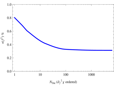
Figure 4: Relative error in $f^{2}$ as a function of the number of data ordered according to a decreasing Hessian value.

V.6 Systematics as a function of the number of data

As already mentioned, the Granada-2013 database is $3\sigma$-self consistent according to our coarse grained PWA. That implies that we can treat measurements as independent. On the other hand we expect the precision will increase with the number of data. Of course, our selection of data is susceptible to change by gathering more data in the future. The Cramer-Rao inequality provides a lower bound on the error on the fitting parameters which can be determined from least squares fitting evans2004probability . Thus, errors will in general be larger than the $N_{\rm Dat}\to\infty$ case. Given the large amount of data considered in the present analysis it is of utmost relevance to analyze this point in some more detail.

Among the many ways of analyzing the systematic uncertainties a particularly interesting one regards a chronological display of our self-consistent database as a function of the year where data where published and hence on the number of scattering data. This can be seen for pp and pp+np analysis separately in tables 9 and 10 respectively in 5 years intervals. As expected, accuracy improves when the total number of data $N_{\rm Dat}$ included in the analysis are increased. Most remarkable is the fact that, instead of the purely statistical estimate $\Delta f^{2}/f^{2}\sim 1/\sqrt{N_{\rm Dat}}$, a fit to the actual trend reveals more, $\Delta f^{2}/f^{2}=29.3/N_{\rm Dat}$, which is in fact better, see Fig. 5. This may be due to the fact that newer data tends to be more precise than older data. In fact, while the database contains more np data than pp data, the pp data have smaller statistical errors and the corresponding fitting parameters tend to be better determined.

Table 9: The pion-proton-proton coupling constant $f_{p}^{2}$ determined from different fits to the Granada-2013 database including only pp data up to a given year.

Year	$f_{p}^{2}$	$\Delta f_{p}^{2}$	$\chi_{pp}^{2}$	$N_{pp}$	$\chi_{pp}^{2}/N_{pp}$
1960	0.07867	0.00421	459.50	535	0.86
1965	0.07568	0.00210	669.05	748	0.89
1970	0.07273	0.00094	978.78	1137	0.86
1975	0.07317	0.00089	1149.63	1247	0.92
1980	0.07339	0.00069	1486.35	1585	0.94
1985	0.07443	0.00052	1559.43	1648	0.95
1990	0.07528	0.00050	1774.58	1831	0.97
1995	0.07542	0.00049	1809.02	1872	0.97
2000	0.07596	0.00043	2985.70	3003	0.99

Table 10: The pion-nucleon-nucleon coupling constant $f^{2}$ determined from different fits to the Granada-2013 database including only data up to a given year.

Year	$f^{2}$	$\Delta f^{2}$	$\chi_{pp}^{2}$	$N_{pp}$	$\chi^{2}_{np}$	$N_{np}$	$\chi^{2}/N$
1960	0.07860	0.00378	460.07	535	186.92	233	0.84
1965	0.07740	0.00192	671.34	748	791.65	836	0.92
1970	0.07427	0.00088	982.23	1137	922.94	981	0.90
1975	0.07504	0.00082	1156.39	1247	1145.81	1221	0.93
1980	0.07421	0.00061	1492.55	1585	2299.10	2311	0.97
1985	0.07499	0.00046	1580.77	1648	2612.23	2584	0.99
1990	0.07580	0.00043	1786.61	1831	2875.34	2806	1.01
1995	0.07607	0.00039	1821.38	1872	3022.34	2950	1.00
2000	0.07654	0.00034	2996.49	3003	3708.46	3528	1.03
2005	0.07631	0.00034	2995.27	3003	3827.69	3634	1.03
2013	0.07633	0.00014	2995.20	3003	3951.86	3717	1.03

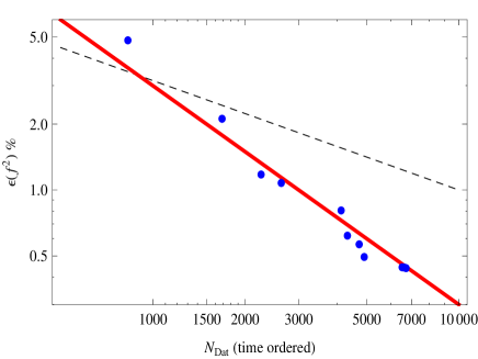
Figure 5: Relative error in $f^{2}$ as a function of the number of data ordered according to their date of publication. Every point represents the number of np+pp scattering data extracted from the Granada-2013 NN database and starting in 1960 forward in 5 years step. We also show the statistical estimate $\epsilon(f^{2})=1/\sqrt{N_{\rm Par}}$ (black,dashed) and the fitting $\epsilon(f^{2})=30/N_{\rm Par}$ (red,solid)

V.7 Summary

The conclusion of all these investigations is that acceptable and natural fits produce smaller errorbars than the purely statistical analysis presented in the previous Section. This is probably due to the optimal sampling of the interaction complying with Nyquist theorem.

VI Conclusions

Since the strong proton-proton and neutron-neutron potentials correspond to the exchange of a neutral pion, the difference in the couplings manifests in the difference of the potentials above the estimated exclusive domain of the CD-OPE interaction. We can illustrate the main result pictorially in Fig. 6 by choosing the transversely and longitudinally polarized protons and neutrons. So we see that in any of the cases considered the strength of the nn potential is stronger than the pp potential, for instance $|V_{n\uparrow,n\uparrow}|>|V_{p\uparrow,p\uparrow}|$ for $r>r_{c}=3{\rm fm}$. Note that we cannot determine the neutron-neutron interaction below $r_{c}$, and in particular the corresponding neutron-neutron scattering length cannot be determined from the present calculation.

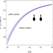
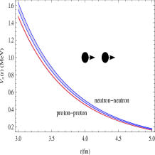
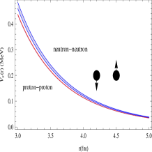
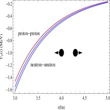
Figure 6: Proton-proton and neutron-neutron interaction above 3fm due to exchange of a neutral pion for different spin polarization states. The bands correspond to the statistical uncertainties from a fit to $6713$np+pp scattering data below $T_{\rm LAB}=350{\rm MeV}$ with $\chi^{2}/\nu=1.039$.

We summarize our points. Using the $3\sigma$ self-consistent Granada-2013 database for np and pp scattering comprising LAB energies below 350 MeV we have investigated isospin breaking in the pion-nucleon coupling constants by separating the nuclear potential in two distinct contributions: Above 3 fm we use charge dependent one pion exchange potential for the strong part along with electromagnetic and relativistic corrections. Below 3 fm we regard the interaction as unknown and we coarse grain it down to the shortest de Broglie wavelength corresponding to pion production threshold which is about 0.6 fm. With a total number of 55 parameters, including the three pion-nucleon coupling constants, we describe a total number of 6741 np and pp data including normalization factors provided by the experimentalist which a total $\chi^{2}$ of 6855.5, which means $\chi^{2}/\nu=1.025$. We see clear evidence that the coupling of neutral pions to neutrons is larger than to protons. As a consequence neutrons interact more strongly than protons.

Appendix A Operator basis

To incorporate charge dependence on $P$ waves two more operators need to be added to the basis we used previously getting a total of $23$ operators $O^{n}$. The potential is written as a sum of functions multiplied by each operator

$$V(r)=\sum_{n=1,23}V_{n}(r)O^{n}$$ (21)

The first fourteen operators are charge independent and correspond to the ones used in the Argonne $v_{14}$ potential

$$O^{n=1,14} = 1,{\tau}_{1}\!\cdot\!{\tau}_{2},\,{\sigma}_{1}\!\cdot\!{\sigma}_{2},({\sigma}_{1}\!\cdot\!{\sigma}_{2})({\tau}_{1}\!\cdot\!{\tau}_{2}),\,S_{12},S_{12}({\tau}_{1}\!\cdot\!{\tau}_{2}),\,$$

$${\bf L}\!\cdot\!{\bf S},{\bf L}\!\cdot\!{\bf S}({\tau}_{1}\!\cdot\!{\tau}_{2}),L^{2},L^{2}({\tau}_{1}\!\cdot\!{\tau}_{2}),\,L^{2}({\sigma}_{1}\!\cdot\!{\sigma}_{2}),$$

$$L^{2}({\sigma}_{1}\!\cdot\!{\sigma}_{2})({\tau}_{1}\!\cdot\!{\tau}_{2}),\,({\bf L}\!\cdot\!{\bf S})^{2},({\bf L}\!\cdot\!{\bf S})^{2}({\tau}_{1}\!\cdot\!{\tau}_{2})\ .$$

These fourteen components are denoted by $c$, $\tau$, $\sigma$, $\sigma\tau$, $t$, $t\tau$, $ls$, $ls\tau$, $l2$, $l2\tau$, $l2\sigma$, $l2\sigma\tau$, $ls2$, and $ls2\tau$. The remaining charge dependent operators are

$$O^{n=15,21} = T_{12},\,({\sigma}_{1}\!\cdot\!{\sigma}_{2})T_{12}\,,S_{12}T_{12},\,(\tau_{z1}+\tau_{z2})\ ,$$ (23)

$$({\sigma}_{1}\!\cdot\!{\sigma}_{2})(\tau_{z1}+\tau_{z2})\ ,L^{2}T_{12},L^{2}({\sigma}_{1}\!\cdot\!{\sigma}_{2})T_{12}\,.$$

$${\bf L}\!\cdot\!{\bf S}T_{12},({\bf L}\!\cdot\!{\bf S})^{2}T_{12}$$

and are labeled as $T$, $\sigma T$,$tT$, $\tau z$,$\sigma\tau z$, $l2T$, $l2\sigma T$, $lsT$ and $ls2T$. The first five were introduced by Wiringa, Stoks and Schiavilla in Wiringa:1994wb ; the following two were included in Perez:2013jpa to restrict the charge dependence to the ${}^{1}S_{0}$ by following certain linear dependence relations between $V_{T}$, $V_{\sigma T}$, $V_{l2T}$ and $V_{l2\sigma T}$. The last two terms are required for the charge dependence on the ${}^{3}P_{0}$, ${}^{3}P_{1}$ and ${}^{3}P_{2}$ partial waves.

As in our previous analysis we set $V_{tT}=V_{\tau z}=V_{\sigma\tau z}=0$ to exclude charge dependence on the tensor terms and charge asymmetries. To restrict the charge dependence to the $S$ and $P$ waves parameters the remaining potential functions must follow

$$48V_{l2T} = -5V_{T}+3V_{\sigma T}+12V_{lsT}-48V_{ls2T}$$ (24)

$$48V_{\sigma l2T} = V_{T}-7V_{\sigma T}+4V_{lsT}-16V_{ls2T}$$ (25)

Appendix B Phase-shifts

Here we provide the pp and np phase-shifts for the lower partial waves and selected LAB energies with their corresponding errorbars for the fit with charge dependence in S and P waves. In the case that errors are smaller than $10^{-3}$ we just represent it by the symbol $-$.

Table 11: pp isovector phaseshifts.

$E_{\rm LAB}$	${}^{1}S_{0}$	${}^{1}D_{2}$	${}^{1}G_{4}$	${}^{3}P_{0}$	${}^{3}P_{1}$	${}^{3}F_{3}$	${}^{3}P_{2}$	$\epsilon_{2}$	${}^{3}F_{2}$	${}^{3}F_{4}$	$\epsilon_{4}$	${}^{3}H_{4}$
1	$32.674$	$0.001$	$0.000$	$0.135$	$-0.081$	$-0.000$	$0.014$	$-0.001$	$0.000$	$0.000$	$-0.000$	$0.000$
	$\pm 0.003$	$-$	$-$	$-$	$-$	$-$	$-$	$-$	$-$	$-$	$-$	$-$
5	$54.836$	$0.043$	$0.000$	$1.599$	$-0.901$	$-0.004$	$0.213$	$-0.052$	$0.002$	$0.000$	$-0.000$	$0.000$
	$\pm 0.008$	$-$	$-$	$\pm 0.005$	$\pm 0.003$	$-$	$\pm 0.001$	$-$	$-$	$-$	$-$	$-$
10	$55.238$	$0.166$	$0.003$	$3.772$	$-2.054$	$-0.032$	$0.648$	$-0.204$	$0.013$	$0.001$	$-0.004$	$0.000$
	$\pm 0.011$	$\pm 0.001$	$-$	$\pm 0.011$	$\pm 0.006$	$-$	$\pm 0.002$	$\pm 0.001$	$-$	$-$	$-$	$-$
25	$48.759$	$0.699$	$0.040$	$8.666$	$-4.888$	$-0.234$	$2.490$	$-0.820$	$0.107$	$0.019$	$-0.050$	$0.004$
	$\pm 0.014$	$\pm 0.002$	$-$	$\pm 0.027$	$\pm 0.010$	$\pm 0.001$	$\pm 0.006$	$\pm 0.003$	$\pm 0.001$	$-$	$-$	$-$
50	$39.133$	$1.711$	$0.154$	$11.577$	$-8.224$	$-0.696$	$5.856$	$-1.719$	$0.346$	$0.104$	$-0.200$	$0.027$
	$\pm 0.018$	$\pm 0.004$	$\pm 0.001$	$\pm 0.046$	$\pm 0.013$	$\pm 0.004$	$\pm 0.011$	$\pm 0.005$	$\pm 0.002$	$\pm 0.001$	$\pm 0.001$	$-$
100	$25.340$	$3.774$	$0.422$	$9.535$	$-13.260$	$-1.502$	$10.986$	$-2.650$	$0.842$	$0.466$	$-0.561$	$0.112$
	$\pm 0.036$	$\pm 0.009$	$\pm 0.002$	$\pm 0.072$	$\pm 0.021$	$\pm 0.010$	$\pm 0.024$	$\pm 0.009$	$\pm 0.009$	$\pm 0.005$	$\pm 0.002$	$\pm 0.001$
150	$15.116$	$5.618$	$0.703$	$4.839$	$-17.637$	$-2.077$	$14.021$	$-2.921$	$1.203$	$1.019$	$-0.883$	$0.225$
	$\pm 0.050$	$\pm 0.015$	$\pm 0.006$	$\pm 0.079$	$\pm 0.027$	$\pm 0.020$	$\pm 0.023$	$\pm 0.013$	$\pm 0.017$	$\pm 0.010$	$\pm 0.003$	$\pm 0.002$
200	$6.892$	$7.206$	$1.000$	$-0.214$	$-21.554$	$-2.471$	$15.803$	$-2.907$	$1.334$	$1.638$	$-1.133$	$0.351$
	$\pm 0.060$	$\pm 0.022$	$\pm 0.012$	$\pm 0.071$	$\pm 0.039$	$\pm 0.037$	$\pm 0.027$	$\pm 0.017$	$\pm 0.023$	$\pm 0.017$	$\pm 0.005$	$\pm 0.006$
250	$0.178$	$8.552$	$1.295$	$-5.098$	$-24.984$	$-2.623$	$16.739$	$-2.698$	$1.224$	$2.205$	$-1.311$	$0.479$
	$\pm 0.075$	$\pm 0.025$	$\pm 0.017$	$\pm 0.068$	$\pm 0.055$	$\pm 0.054$	$\pm 0.034$	$\pm 0.023$	$\pm 0.029$	$\pm 0.024$	$\pm 0.006$	$\pm 0.013$
300	$-5.222$	$9.571$	$1.571$	$-9.601$	$-27.919$	$-2.418$	$16.981$	$-2.293$	$0.918$	$2.659$	$-1.439$	$0.591$
	$\pm 0.102$	$\pm 0.032$	$\pm 0.019$	$\pm 0.095$	$\pm 0.070$	$\pm 0.066$	$\pm 0.034$	$\pm 0.032$	$\pm 0.041$	$\pm 0.029$	$\pm 0.008$	$\pm 0.020$
350	$-9.447$	$10.140$	$1.832$	$-13.545$	$-30.348$	$-1.820$	$16.635$	$-1.707$	$0.454$	$3.012$	$-1.552$	$0.670$
	$\pm 0.138$	$\pm 0.055$	$\pm 0.027$	$\pm 0.152$	$\pm 0.082$	$\pm 0.080$	$\pm 0.031$	$\pm 0.042$	$\pm 0.058$	$\pm 0.047$	$\pm 0.010$	$\pm 0.027$

Table 12: np isovector phaseshifts.

$E_{\rm LAB}$	${}^{1}S_{0}$	${}^{1}D_{2}$	${}^{1}G_{4}$	${}^{3}P_{0}$	${}^{3}P_{1}$	${}^{3}F_{3}$	${}^{3}P_{2}$	$\epsilon_{2}$	${}^{3}F_{2}$	${}^{3}F_{4}$	$\epsilon_{4}$	${}^{3}H_{4}$
1	$62.047$	$0.001$	$0.000$	$0.183$	$-0.105$	$-0.000$	$0.025$	$-0.001$	$0.000$	$0.000$	$-0.000$	$0.000$
	$\pm 0.024$	$-$	$-$	$\pm 0.003$	$\pm 0.002$	$-$	$-$	$-$	$-$	$-$	$-$	$-$
5	$63.559$	$0.041$	$0.000$	$1.683$	$-0.911$	$-0.004$	$0.284$	$-0.049$	$0.002$	$0.000$	$-0.000$	$0.000$
	$\pm 0.046$	$\pm 0.001$	$-$	$\pm 0.029$	$\pm 0.016$	$-$	$\pm 0.004$	$\pm 0.001$	$-$	$-$	$-$	$-$
10	$59.851$	$0.155$	$0.002$	$3.823$	$-1.996$	$-0.026$	$0.796$	$-0.185$	$0.011$	$0.001$	$-0.003$	$0.000$
	$\pm 0.053$	$\pm 0.003$	$-$	$\pm 0.058$	$\pm 0.031$	$\pm 0.001$	$\pm 0.009$	$\pm 0.004$	$-$	$-$	$-$	$-$
25	$50.712$	$0.673$	$0.032$	$8.699$	$-4.666$	$-0.195$	$2.846$	$-0.765$	$0.091$	$0.017$	$-0.040$	$0.003$
	$\pm 0.062$	$\pm 0.012$	$\pm 0.001$	$\pm 0.096$	$\pm 0.053$	$\pm 0.005$	$\pm 0.027$	$\pm 0.014$	$\pm 0.002$	$\pm 0.001$	$\pm 0.001$	$-$
50	$40.225$	$1.695$	$0.134$	$11.682$	$-7.822$	$-0.594$	$6.364$	$-1.660$	$0.309$	$0.105$	$-0.170$	$0.021$
	$\pm 0.083$	$\pm 0.019$	$\pm 0.003$	$\pm 0.109$	$\pm 0.059$	$\pm 0.015$	$\pm 0.045$	$\pm 0.020$	$\pm 0.006$	$\pm 0.004$	$\pm 0.004$	$\pm 0.001$
100	$26.129$	$3.760$	$0.391$	$9.484$	$-12.592$	$-1.299$	$11.070$	$-2.658$	$0.780$	$0.514$	$-0.507$	$0.095$
	$\pm 0.138$	$\pm 0.018$	$\pm 0.009$	$\pm 0.163$	$\pm 0.080$	$\pm 0.036$	$\pm 0.061$	$\pm 0.009$	$\pm 0.013$	$\pm 0.021$	$\pm 0.011$	$\pm 0.002$
150	$15.917$	$5.568$	$0.671$	$4.399$	$-16.716$	$-1.915$	$13.334$	$-3.000$	$1.117$	$1.130$	$-0.828$	$0.204$
	$\pm 0.191$	$\pm 0.017$	$\pm 0.013$	$\pm 0.216$	$\pm 0.120$	$\pm 0.062$	$\pm 0.082$	$\pm 0.020$	$\pm 0.020$	$\pm 0.039$	$\pm 0.015$	$\pm 0.005$
200	$7.810$	$7.118$	$0.961$	$-1.038$	$-20.374$	$-2.536$	$14.510$	$-3.028$	$1.217$	$1.773$	$-1.091$	$0.334$
	$\pm 0.243$	$\pm 0.023$	$\pm 0.017$	$\pm 0.261$	$\pm 0.170$	$\pm 0.085$	$\pm 0.109$	$\pm 0.027$	$\pm 0.024$	$\pm 0.054$	$\pm 0.014$	$\pm 0.011$
250	$1.289$	$8.435$	$1.238$	$-6.196$	$-23.543$	$-2.989$	$15.158$	$-2.834$	$1.072$	$2.318$	$-1.290$	$0.464$
	$\pm 0.302$	$\pm 0.025$	$\pm 0.020$	$\pm 0.304$	$\pm 0.224$	$\pm 0.101$	$\pm 0.125$	$\pm 0.030$	$\pm 0.030$	$\pm 0.070$	$\pm 0.010$	$\pm 0.018$
300	$-3.856$	$9.421$	$1.488$	$-10.830$	$-26.215$	$-2.958$	$15.386$	$-2.426$	$0.733$	$2.732$	$-1.441$	$0.561$
	$\pm 0.367$	$\pm 0.033$	$\pm 0.021$	$\pm 0.356$	$\pm 0.274$	$\pm 0.135$	$\pm 0.122$	$\pm 0.036$	$\pm 0.042$	$\pm 0.090$	$\pm 0.008$	$\pm 0.027$
350	$-7.791$	$9.947$	$1.720$	$-14.770$	$-28.375$	$-2.224$	$15.185$	$-1.828$	$0.244$	$3.053$	$-1.574$	$0.593$
	$\pm 0.439$	$\pm 0.057$	$\pm 0.028$	$\pm 0.427$	$\pm 0.318$	$\pm 0.250$	$\pm 0.107$	$\pm 0.045$	$\pm 0.059$	$\pm 0.126$	$\pm 0.011$	$\pm 0.036$

Table 13: np isoscalar phaseshifts.

$E_{\rm LAB}$	${}^{1}P_{1}$	${}^{1}F_{3}$	${}^{3}D_{2}$	${}^{3}G_{4}$	${}^{3}S_{1}$	$\epsilon_{1}$	${}^{3}D_{1}$	${}^{3}D_{3}$	$\epsilon_{3}$	${}^{3}G_{3}$
1	$-0.191$	$-0.000$	$0.006$	$0.000$	$147.685$	$0.105$	$-0.005$	$0.000$	$0.000$	$-0.000$
	$-$	$-$	$-$	$-$	$\pm 0.017$	$\pm 0.001$	$-$	$-$	$-$	$-$
5	$-1.528$	$-0.010$	$0.226$	$0.001$	$118.043$	$0.654$	$-0.186$	$0.002$	$0.013$	$-0.000$
	$\pm 0.003$	$-$	$-$	$-$	$\pm 0.024$	$\pm 0.005$	$-$	$-$	$-$	$-$
10	$-3.119$	$-0.066$	$0.876$	$0.012$	$102.425$	$1.112$	$-0.690$	$0.005$	$0.083$	$-0.003$
	$\pm 0.009$	$-$	$\pm 0.001$	$-$	$\pm 0.034$	$\pm 0.011$	$\pm 0.002$	$-$	$-$	$-$
25	$-6.413$	$-0.435$	$3.839$	$0.177$	$80.364$	$1.696$	$-2.843$	$0.039$	$0.572$	$-0.055$
	$\pm 0.029$	$-$	$\pm 0.010$	$-$	$\pm 0.059$	$\pm 0.026$	$\pm 0.009$	$\pm 0.001$	$-$	$-$
50	$-9.656$	$-1.173$	$9.265$	$0.755$	$62.489$	$2.032$	$-6.496$	$0.292$	$1.658$	$-0.274$
	$\pm 0.062$	$\pm 0.002$	$\pm 0.037$	$\pm 0.001$	$\pm 0.078$	$\pm 0.047$	$\pm 0.026$	$\pm 0.005$	$\pm 0.004$	$\pm 0.001$
100	$-14.214$	$-2.304$	$17.776$	$2.321$	$43.135$	$2.515$	$-12.295$	$1.321$	$3.532$	$-1.007$
	$\pm 0.097$	$\pm 0.015$	$\pm 0.076$	$\pm 0.014$	$\pm 0.086$	$\pm 0.082$	$\pm 0.054$	$\pm 0.020$	$\pm 0.018$	$\pm 0.011$
150	$-18.203$	$-3.097$	$22.620$	$3.986$	$30.862$	$2.927$	$-16.683$	$2.338$	$4.833$	$-1.873$
	$\pm 0.114$	$\pm 0.036$	$\pm 0.096$	$\pm 0.045$	$\pm 0.098$	$\pm 0.110$	$\pm 0.081$	$\pm 0.042$	$\pm 0.031$	$\pm 0.036$
200	$-21.765$	$-3.831$	$24.866$	$5.583$	$21.462$	$3.272$	$-20.284$	$2.931$	$5.790$	$-2.718$
	$\pm 0.142$	$\pm 0.053$	$\pm 0.123$	$\pm 0.080$	$\pm 0.123$	$\pm 0.131$	$\pm 0.114$	$\pm 0.067$	$\pm 0.040$	$\pm 0.064$
250	$-24.856$	$-4.634$	$25.699$	$7.011$	$13.557$	$3.677$	$-23.290$	$3.067$	$6.565$	$-3.516$
	$\pm 0.181$	$\pm 0.061$	$\pm 0.149$	$\pm 0.102$	$\pm 0.148$	$\pm 0.142$	$\pm 0.130$	$\pm 0.095$	$\pm 0.055$	$\pm 0.083$
300	$-27.487$	$-5.498$	$25.991$	$8.197$	$6.566$	$4.262$	$-25.639$	$2.870$	$7.195$	$-4.314$
	$\pm 0.221$	$\pm 0.077$	$\pm 0.194$	$\pm 0.117$	$\pm 0.171$	$\pm 0.175$	$\pm 0.143$	$\pm 0.129$	$\pm 0.069$	$\pm 0.101$
350	$-29.666$	$-6.335$	$26.295$	$9.101$	$0.223$	$5.068$	$-27.156$	$2.492$	$7.647$	$-5.173$
	$\pm 0.257$	$\pm 0.129$	$\pm 0.312$	$\pm 0.142$	$\pm 0.193$	$\pm 0.265$	$\pm 0.210$	$\pm 0.166$	$\pm 0.082$	$\pm 0.146$

References

- (1) H. Yukawa, Proc. Phys. Math. Soc. Jap. 17 (1935) 48, [Prog. Theor. Phys. Suppl.1,1(1935)].
- (2) W. Pauli, Meson theory of nuclear forces (Interscience Publishers, 1948).
- (3) O. Dumbrajs et al., Nucl.Phys. B216 (1983) 277.
- (4) J. de Swart, M. Rentmeester and R. Timmermans, PiN Newslett. 13 (1997) 96, nucl-th/9802084.
- (5) M. Sainio, PiN Newslett. 15 (1999) 156, hep-ph/9912337.
- (6) D. Bugg, Eur.Phys.J. C33 (2004) 505.
- (7) H.A. Bethe, Phys. Rev. 57 (1940) 260.
- (8) H. Bethe, Phys.Rev. 57 (1940) 390.
- (9) M.L. Goldberger and S.B. Treiman, Phys. Rev. 110 (1958) 1178.
- (10) Y. Nambu, Phys. Rev. Lett. 4 (1960) 380.
- (11) G.F. Chew, Phys. Rev. 112 (1958) 1380.
- (12) P. Cziffra et al., Phys. Rev. 114 (1959) 880.
- (13) M.H. MacGregor, M.J. Moravcsik and H.P. Stapp, Phys. Rev. 116 (1959) 1248.
- (14) P.S. Signell, Phys. Rev. Lett. 5 (1960) 474.
- (15) M. MacGregor, R. Arndt and A. Dubow, Physical Review 135 (1964) B628.
- (16) D.V. Bugg, A.A. Carter and J.R. Carter, Phys. Lett. B44 (1973) 278.
- (17) R.A. Arndt et al., Phys. Rev. Lett. 65 (1990) 157.
- (18) R. Arndt, R. Workman and M. Pavan, Phys.Rev. C49 (1994) 2729.
- (19) T.E.O. Ericson, B. Loiseau and A.W. Thomas, Phys.Rev. C66 (2002) 014005, hep-ph/0009312.
- (20) R.A. Arndt et al., Phys. Rev. C74 (2006) 045205, nucl-th/0605082.
- (21) V. Baru et al., Phys.Lett. B694 (2011) 473, 1003.4444.
- (22) V. Baru et al., Nucl.Phys. A872 (2011) 69, 1107.5509.
- (23) R.G.E. Timmermans, T.A. Rijken and J.J. de Swart, Phys. Rev. Lett. 67 (1991) 1074.
- (24) V. Stoks et al., Phys.Rev. C48 (1993) 792.
- (25) R. Klomp, V. Stoks and J. de Swart, Phys.Rev. C44 (1991) 1258.
- (26) V.G. Stoks, R. Timmermans and J. de Swart, Phys.Rev. C47 (1993) 512, nucl-th/9211007.
- (27) N. Kaiser, R. Brockmann and W. Weise, Nucl. Phys. A625 (1997) 758, nucl-th/9706045.
- (28) M.C.M. Rentmeester et al., Phys. Rev. Lett. 82 (1999) 4992, nucl-th/9901054.
- (29) M.C.M. Rentmeester, R.G.E. Timmermans and J.J. de Swart, Phys. Rev. C67 (2003) 044001, nucl-th/0302080.
- (30) M.J. Evans and J.S. Rosenthal, Probability and statistics: The science of uncertainty (Macmillan, 2004).
- (31) J. Dobaczewski, W. Nazarewicz and P.G. Reinhard, J. Phys. G41 (2014) 074001, 1402.4657.
- (32) J. Bergervoet et al., Phys.Rev. C38 (1988) 15.
- (33) R. Navarro Pérez, J.E. Amaro and E. Ruiz Arriola, Few Body Syst. 55 (2014) 983, 1310.8167.
- (34) R. Navarro Pérez, J.E. Amaro and E. Ruiz Arriola, Phys. Rev. C88 (2013) 064002, 1310.2536, [Erratum: Phys. Rev.C91,no.2,029901(2015)].
- (35) R. Navarro Pérez, J.E. Amaro and E. Ruiz Arriola, Phys. Rev. C89 (2014) 064006, 1404.0314.
- (36) R. Navarro Pérez, J.E. Amaro and E. Ruiz Arriola, J. Phys. G42 (2015) 034013, 1406.0625.
- (37) S. Aldor-Noiman et al., Amer. Statist. 67 (2013) 249.
- (38) R. Navarro Pérez, E. Ruiz Arriola and J. Ruiz de Elvira, Phys. Rev. D91 (2015) 074014, 1502.03361.
- (39) T.E.O. Ericson et al., Phys. Rev. Lett. 75 (1995) 1046.
- (40) J. Rahm et al., Phys. Rev. C57 (1998) 1077.
- (41) S. Weinberg, The quantum theory of fields. Vol. 2: Modern applications (Cambridge University Press, 2013).
- (42) M.C.M. Rentmeester, R.A.M. Klomp and J.J. de Swart, Phys. Rev. Lett. 81 (1998) 5253, nucl-th/9812020.
- (43) T.E.O. Ericson et al., Phys. Rev. Lett. 81 (1998) 5254.
- (44) J. Blomgren, editor, Critical issues in the determination of the pion nucleon coupling constant. Proceedings, Workshop, Uppsala, Sweden, June 7-8, 1999 Vol. T87, 2000.
- (45) M. Sarsour et al., Phys. Rev. Lett. 94 (2005) 082303, nucl-ex/0412026.
- (46) M. Sarsour et al., Phys. Rev. C74 (2006) 044003, nucl-ex/0602017.
- (47) Sinya AOKI for HAL QCD Collaboration, S. Aoki, Prog.Part.Nucl.Phys. 66 (2011) 687, 1107.1284.
- (48) S. Aoki, Eur.Phys.J. A49 (2013) 81, 1309.4150.
- (49) S. Aoki, T. Hatsuda and N. Ishii, Prog.Theor.Phys. 123 (2010) 89, 0909.5585.
- (50) J.B. Aviles, Phys. Rev. C6 (1972) 1467.
- (51) R.N. Perez, J.E. Amaro and E. Ruiz Arriola, Int. J. Mod. Phys. E25 (2016) 1641009, 1601.08220.
- (52) C.A. Dominguez, Riv. Nuovo Cim. 8N6 (1985) 1.
- (53) J.L. Goity et al., Phys.Lett. B454 (1999) 115, hep-ph/9901374.
- (54) J. Goity and J. Saez, report JLAB-THY-03-26 (2002).
- (55) V. Bernard, N. Kaiser and U.G. Meissner, Nucl. Phys. A615 (1997) 483, hep-ph/9611253.
- (56) T. Ledwig et al., Phys. Rev. D90 (2014) 114020, 1407.3750.
- (57) A.W. Thomas and K. Holinde, Phys.Rev.Lett. 63 (1989) 2025.
- (58) R. Braun et al., Phys.Lett. B660 (2008) 161, 0801.4600.
- (59) F. Gross and A. Stadler, Phys.Lett. B668 (2008) 163, 0808.2962.
- (60) G. Weisel, R. Braun and W. Tornow, Phys.Rev. C82 (2010) 027001.
- (61) R.B. Wiringa, V. Stoks and R. Schiavilla, Phys.Rev. C51 (1995) 38, nucl-th/9408016.
- (62) R. Machleidt, Phys.Rev. C63 (2001) 024001, nucl-th/0006014.
- (63) R. Navarro Pérez, J.E. Amaro and E. Ruiz Arriola, Phys. Rev. C89 (2014) 024004, 1310.6972.
- (64) R. Navarro Pérez, J.E. Amaro and E. Ruiz Arriola, Phys. Rev. C88 (2013) 024002, 1304.0895, [Erratum: Phys. Rev.C88,no.6,069902(2013)].
- (65) V. Stoks and J.J. de Swart, Phys. Rev. C47 (1993) 761.
- (66) V.G.J. Stoks and J.J. de Swart, Phys. Rev. C52 (1995) 1698, nucl-th/9411002.
- (67) N. Hoshizaki, Prog. Theor. Phys. Suppl. 42 (1969) 107.
- (68) J. Bystricky, F. Lehar and P. Winternitz, J. Phys.(France) 39 (1978) 1.
- (69) E. Ruiz Arriola, J.E. Amaro and R. Navarro Pérez, Mod. Phys. Lett. A31 (2016) 1630027, 1606.02171.
- (70) R. Navarro Pérez, J.E. Amaro and E. Ruiz Arriola, Phys. Rev. C91 (2015) 054002, 1411.1212.
- (71) E. Ruiz Arriola, J.E. Amaro and R. Navarro Perez, EPJ Web Conf. 137 (2017) 09006, 1611.02607.
- (72) R. Navarro Pérez, J.E. Amaro and E. Ruiz Arriola, J. Phys. G43 (2016) 114001, 1410.8097.
- (73) I. Ruiz Simo et al., (2016), 1612.06228.
- (74) R. Navarro Pérez, J.E. Amaro and E. Ruiz Arriola, PoS CD12 (2013) 104, 1301.6949.
- (75) D. Siemens et al., (2016), 1610.08978.