PEXSI-: A Green’s function embedding method for Kohn-Sham density functional theory
Abstract.
In this paper, we propose a new Green’s function embedding method called PEXSI- for describing complex systems within the Kohn-Sham density functional theory (KSDFT) framework, after revisiting the physics literature of Green’s function embedding methods from a numerical linear algebra perspective. The PEXSI- method approximates the density matrix using a set of nearly optimally chosen Green’s functions evaluated at complex frequencies. For each Green’s function, the complex boundary conditions are described by a self energy matrix constructed from a physical reference Green’s function, which can be computed relatively easily. In the linear regime, such treatment of the boundary condition can be numerically exact. The support of the matrix is restricted to degrees of freedom near the boundary of computational domain, and can be interpreted as a frequency dependent surface potential. This makes it possible to perform KSDFT calculations with computational complexity, where is the number of atoms within the computational domain. Green’s function embedding methods are also naturally compatible with atomistic Green’s function methods for relaxing the atomic configuration outside the computational domain. As a proof of concept, we demonstrate the accuracy of the PEXSI- method for graphene with divacancy and dislocation dipole type of defects using the DFTB+ software package.
1. Introduction
This paper concerns the simulation of defects in materials in the framework of Kohn-Sham density functional theory (KSDFT) [HohenbergKohn1964, KohnSham1965]. Here we use the term “defect” to refer to general local perturbations such as vacancies, dislocations, in the otherwise smoothly deformed lattice structure in materials. We are interested in cases that the global system is too large to be modeled entirely by KSDFT, so that we can only afford to “embed” the defect in an auxiliary system, in which the number of degrees of freedom is comparable to that of the defect region itself. In physics literature this procedure is known as “embedding”. In the context of KSDFT, the goal of embedding is to correctly evaluate the density matrix corresponding to the defect region. The simplest embedding scheme only includes the defect together with some nearby degrees of freedom, and places the resulting auxiliary system in vacuum. This scheme often leads to large error for real materials simulation. Practically used embedding schemes often modify the degrees of freedom near the boundary of the auxiliary system to mimic the materials environment. Analogous to the setup in partial differential equations (PDEs), we view such modification as a “boundary condition”. One common procedure is to embed the defects in a “supercell”, so that the auxiliary system is periodically extended. In the past two decades, the supercell approaches, such as those based on planewave basis sets [PayneTeterAllenEtAl1992, KresseFurthmuller1996, MakovPayne1995], have been the most widely used methods in computational material science to model defects. On the other hand, many systems are not periodic to start with, and the inherent periodic boundary treatment in supercell approaches is therefore not always suitable. Quantum transport, defect migration, defect-defect interaction, and dislocations are just a few examples of scenarios where the periodic boundary condition encounters significant difficulties.
Various embedding schemes [Cortona1991, KniziaChan2013, GoodpasterAnanthManbyEtAl2010, HuangPavoneCarter2011, GarciaLuE:07, ChenOrtner2015] have been developed in the literature in order to model complex material structures more efficiently without using the periodic boundary conditions. Such methods allow the defect region to be treated not only at the level of KSDFT, but also at higher levels of electronic structure methods such as the coupled cluster theory, though the accuracy of the latter approach of embedding is significantly more difficult to analyze from a numerical analysis perspective. In this paper we focus on Green’s function methods [BernholcLipariPantelides1978, ZellerDederichs1979, WilliamsFeibelmanLang1982, KellyCar92, ZgidChan2011, KananenkaGullZgid2015, NguyenKananenkaZgid2016, ChibaniRenSchefflerEtAl2016, LinLuYingEtAl2009, LinChenYangEtAl2013], and treat the defect region at the level of KSDFT. Green’s function methods evaluate the density matrix through the linear combination of a number of Green’s functions evaluated at complex frequencies. Since they allow a more versatile treatment of complex boundary conditions, they offer an attractive alternative to describe complex systems. In particular, they have been successfully applied to real materials simulation when localized basis functions are available. Examples of Green’s function methods include the locally self-consistent multiple scattering (LSMS) method [WangStocksSheltonEtAl1995, NicholsonStocksWangEtAl1994], Fermi operator expansion method [GoedeckerTeter1995, Goedecker:99], the recent extension of the Korringa-Kohn-Rostoker (KKR) method [ZellerDeutzDederichs1982, ZellerDederichsUjfalussyEtAl1995] called KKRnano [ThiessZellerBoltenEtAl2012], and the PEXSI method [LinLuYingEtAl2009, LinChenYangEtAl2013].
Contribution:
In this work, we consider defects embedded in a physical reference system such as a crystal, modeled at the level of KSDFT. We assume the Hamiltonian operator is discretized using a local basis set, and that we can obtain a number of Green’s functions for the reference system evaluated at different complex frequencies . These reference Green’s functions can be obtained, for instance, by means of a band structure calculation using the periodicity of the reference problem. Then we propose a method to model the defects by an auxiliary system, which contains the defect and a minimal set of degrees of freedom defined according to the sparsity of the Hamiltonian operator. The Hamiltonian operator for this auxiliary system is constructed by the Hamiltonian operator of the global system restricted to the auxiliary system, plus a frequency-dependent term that only modifies a submatrix corresponding to boundary degrees of freedom. This extra term is closely related to a Schur complement, and can be interpreted as a discrete version of the Dirichlet-to-Neumann (DtN) map operator for the global system [EngquistMajda1977, GivoliPatlashenkoKeller1998, KellerGivoli1989]. In physics literature, such modification is a special type of “self energy” contribution. Following standard notation in physics, we denote this extra term by , where is a complex frequency at which the Green’s function needs to be evaluated. We demonstrate that in the linear regime, i.e., in the absence of self-consistent-field (SCF) iteration, our scheme provides a numerically exact density matrix restricted to the defect region. In such case, there is no error in computing physical observables such as the atomic force in the defect region.
Since is only nonzero at the boundary of the auxiliary system, we can efficiently evaluate for the auxiliary system using the pole expansion and selected inversion (PEXSI) method [LinLuYingE2009, LinLuYingEtAl2009, LinYangMezaEtAl2011, LinChenYangEtAl2013]. The computational complexity of the PEXSI method is at most , where is the number of atoms within the computational domain. The PEXSI method does not rely on the near-sightedness principle [Kohn1996], but only relies on the sparsity of the Hamiltonian matrix. Hence the PEXSI method is applicable to metallic systems at room temperature. The PEXSI method can be scalable on massively parallel computers [JacquelinLinYang2015, JacquelinLinWichmannEtAl2015]. PEXSI has been integrated into a number of electronic structure software packages such as SIESTA [LinGarciaHuhsEtAl2014, SolerArtachoGaleEtAl2002], BigDFT [MohrRatcliffBoulangerEtAl2014], CP2K [VandeVondeleKrackMohamedEtAl2005] and DGDFT [LinLuYingE2012, HuLinYang2015a], and has been used for accelerating materials simulation with atoms or more [HuLinYangEtAl2014, HuLinYangEtAl2016].
PEXSI is a Green’s function method for solving KSDFT for the global system, and our development can be naturally combined with the PEXSI method, which is referred to as the PEXSI- method. The modification introduced in this work only modifies matrix elements of the Hamiltonian corresponding to boundary degrees of freedom, which allows us to solve the auxiliary system with at most cost, where is the number of atoms in the auxiliary system. We also present how to combine the PEXSI- method seamlessly with atomistic Green’s function methods [Li2009b, Li2012] for structural relaxation of the defect system.
As a proof of concept, we implement the PEXSI- method in the DFTB+ software package [AradiHourahineFrauenheim2007], and demonstrate the accuracy using a water dimer, graphene with divacancy, and graphene with a dislocation dipole with relaxed geometric structure without SCF iterations. Our numerical results indicate that the PEXSI- method can obtain accurate description of the energy and forces in the defect region.
Related work:
In physics literature, the “self energy” matrix (or matrix) has been used in the context of the non-equilibrium Green’s function (NEGF) method in quantum transport calculations (e.g. [BrandbygeMozosOrdejonEtAl2002]). Both the PEXSI- approach and the NEGF approach modify the boundary degrees of freedom through Schur complements, but there are important differences. In the context of modeling local defects in a crystal, the strategy in the NEGF approach would require the Green’s function corresponding to a crystal but with the defect region removed. The resulting system resembles a crystal with a “hole” corresponding to the defect region, and this unphysical system can be very difficult to solve. On the other hand, PEXSI- only requires the knowledge of Green’s functions for the physical crystal configuration, and such Green’s functions are much easier to compute. In fact, we think our strategy for constructing matrices could be potentially beneficial in the context of quantum transport calculations as well for certain systems. Another type of Green’s function embedding methods use the Dyson equation (e.g. [WilliamsFeibelmanLang1982, KellyCar92]), which uses physical reference Green’s functions. However, the Dyson equation requires dense linear algebra to be performed over the entire auxiliary system, and the computational cost is therefore , where is the number of atoms in the auxiliary system. Meanwhile, PEXSI- only modifies the Hamiltonian matrix corresponding to boundary degrees of freedom and is hence more efficient. Our method is also related to the embedding method proposed by Inglesfield [Inglesfield1981], which is based on matching the boundary condition for each individual eigenfunction. This strategy could be viable when eigenfunctions are well separated from each other spectrally. However, when eigenfunctions are clustered such as for large scale KSDFT calculations, it becomes impractical to derive the boundary condition for each eigenfunction.
We note that the spirit of Green’s function embedding methods are very different from that of the quantum mechanics / molecular mechanics (QM/MM) method, which is widely used in chemistry and biology [WarshelLevitt1976]. In the QM/MM method, the coupling of the two types of models is usually a significant challenge. While QM models involve the degrees of freedom associated with electrons (for example, electron density or electron orbital functions), MM models do not explicitly take into account those degrees of freedom. One intuitive way to understand the issue at the boundary is that the decomposition of the domain into QM and MM regions creates “dangling bonds” at the interface. Therefore, a popular approach is to introduce hydrogen-type atoms to passivate those bonds. More advanced approaches have been proposed to further reduce the artifacts introduced by the coupling. See for example the review articles [GaoTruhlar:02, LinTruhlar:07, SennThiel:09, BrunkRothlisberger:15]. We remark that the bond passivation model becomes challenging in materials science simulations, such as the description of a local defect in aluminum. In Green’s function embedding methods, the coupling is through the boundary conditions imposed on the Green’s function of the QM domain, rather than changing the local chemical environment of the coupling region. In particular, no bond passivation is required.
Organization:
The manuscript is organized as follows. We briefly introduce Kohn-Sham density functional theory and Green’s function methods in section 2, and review existing Green’s function methods from a numerical linear algebra perspective in section 3. In section 4 we introduce a new Green’s function method called PEXSI-, and a geometry relaxation method based on atomistic Green’s functions. We report the numerical results using DFTB+ in section 5, and discuss future directions in section 6.
2. Preliminaries
In Kohn-Sham density functional theory, the ground-state electron charge density of an atomistic system can be obtained from the self-consistent solution to the Kohn-Sham equations
| (1) |
where is the Kohn-Sham Hamiltonian that depends on , and are the Kohn-Sham orbitals. The Kohn-Sham orbitals in turn determine the charge density by
| (2) |
The occupation numbers are chosen according to the Fermi-Dirac distribution function
| (3) |
where is the chemical potential chosen to ensure that
| (4) |
is the inverse temperature, i.e., with being the Boltzmann constant and the temperature. The nonlinear iteration with respect to the electron density can be carried out using a self-consistent-field iteration (SCF) procedure [RMartin].
The electronic-structure problem can be recast in terms of the one-particle density matrix defined by
| (5) |
and the chemical potential chosen so that , which is exactly the same constraint as (4).
To solve for or in practice, we may choose a finite basis set , and use a Galerkin approximation for (1) as the generalized eigenvalue problem
| (6) |
where is the projected Hamiltonian matrix, and is the overlap matrix. The matrix representation of the density matrix, denoted by , can be obtained from the generalized eigenvalue decomposition (6) as
| (7) |
For simplicity we consider the case when real arithmetic is used, and are real symmetric matrices. The extension to the complex Hermitian case is straightforward. Using linear algebra notation, let us denote by the matrix collecting all basis functions. Then the density matrix in the real space can be compactly approximated by
| (8) |
It turns out that, in KSDFT calculations with the local density approximation (LDA) and generalized gradient approximation (GGA) for the exchange-correlation functionals, not all entries of the one-particle density matrix are needed. In order to carry out the self-consistent field iteration, it is sufficient to compute the electron density , the diagonal entries of in the real space, i.e.,
| (9) |
When the basis functions are compactly supported in real space, the product of two functions and is zero when they do not overlap. This leads to sparse Hamiltonian matrix and overlap matrix , respectively. It also implies that in order to compute , we only need such that in Eq. (9). As shall be seen later, such sparsity plays a key role in our method.
The Kohn-Sham equations (1) are well-defined for closed systems such as systems in vacuum (i.e., with Dirichlet boundary condition imposed far away from the system) and with periodic boundary condition. However, the eigenvalue formulation imposes major difficulty for treating open systems. For instance, the embedding of a defect into a crystalline system, which can be a point defect such as a vacancy, or a line defect such as a dislocation. As opposed to the solution of PDEs where tailored boundary conditions can be formulated for specific operators such as in the case of the absorbing boundary condition [EngquistMajda1977], in KSDFT each eigenfunction satisfies a different PDE, and hence requires its own tailored boundary condition. The number of eigenfunctions is proportional to the number of electrons . Finding such boundary conditions is not only expensive when becomes large, but also may not be a stable procedure since the eigenvalues of interest are often clustered, or even form continuous energy bands in the thermodynamic limit for solid state systems.
Here we demonstrate that the one-particle density matrix can serve as a useful tool for quantum embedding. First, can be evaluated without the need for diagonalization, if the Fermi function is approximated by a linear combination of a number of simpler functions. This is the idea behind the Fermi operator expansion (FOE) method [Goedecker1993]. The FOE method is typically used as a linear scaling method to accelerate KSDFT calculations for insulating systems with substantial band gaps, or for general systems under very high temperature. The recently developed pole expansion and selected inversion (PEXSI) method extends the FOE method by means of an efficient rational approximation, and significantly accelerates KSDFT calculations for large scale metallic systems at room temperature [LinLuYingE2009, LinLuYingEtAl2009, LinYangMezaEtAl2011, LinChenYangEtAl2013].
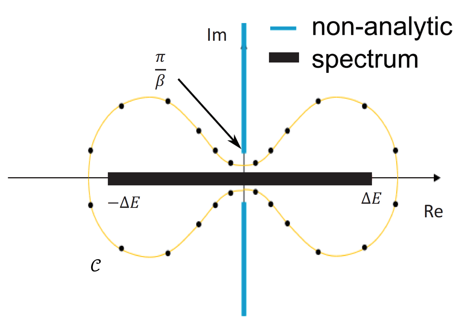
In the PEXSI method, the single particle density matrix can be exactly reformulated by means of a contour integral as
| (10) |
Here can be any contour that encircles the spectrum of without enclosing any pole of the Fermi-Dirac function. In the pole expansion [LinLuYingE2009], we carefully choose a contour as in Fig. 1, and approximate the single particle density matrix by its -term approximation, denoted by as
| (11) |
The complex shifts and weights are determined only by (the spectrum width of the matrix pencil ) and the number of poles . These coefficients are known explicitly and their calculation takes negligible amount of time. The pole expansion is an effective way for approximating the one-particle density matrix, since it requires only terms of simple rational functions. With some abuse of notation, in the following discussion we will drop the subscript originating from the -term pole expansion approximation unless otherwise noted.
Eq. (11) converts the problem of computing the one-particle density matrix by means of eigenfunctions into a problem of evaluating inverse matrices or Green’s functions, defined as
| (12) |
Note that in order to evaluate the electron density, we only need to evaluate the entries such that . This allows the PEXSI method to compute such selected elements of an inverse matrix efficiently. We will discuss more along this line in section 4.1.
3. Existing Green’s function embedding schemes
In the context of embedding, we only need to find the “boundary conditions” for Green’s functions . As mentioned in the introduction, here the term “boundary condition” can refer to a general way of modifying the degrees of freedom in an auxiliary system to mimic the effects of the materials environment. Since is independent of the system size , this becomes a solvable problem even for systems of large sizes. On the other hand, finding proper boundary conditions for eigenvalue problems can become impractical for systems of large sizes [Inglesfield1981]. In this section we first review some existing ideas in the literature, written in consistent linear algebra notation as used in the previous section.
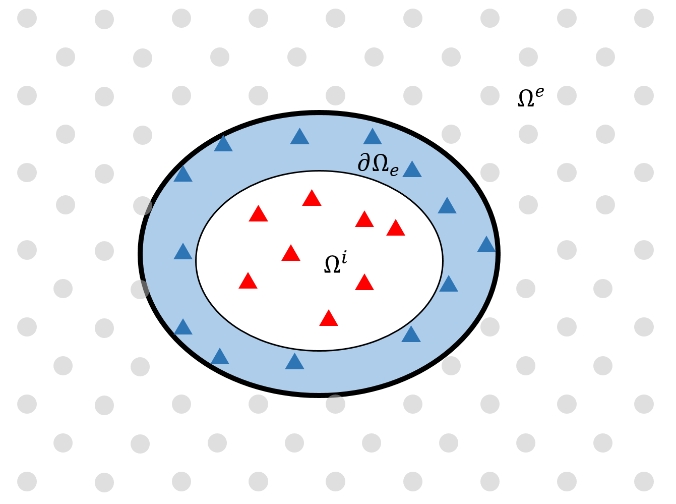
In the embedding scheme, we partition the degrees of freedom (i.e., nodal values associated with the basis functions) into interior degrees of freedom and exterior degrees of freedom , where . In this paper we assume atom-centered basis functions are used in discretizing the Hamiltonian operator. This type of basis set includes atomic orbitals, Gaussian type orbitals, as well as the density-functional tight binding (DFTB) approximation [AradiHourahineFrauenheim2007], which will be used in our numerical examples. With some abuse of notation, we aggregate degrees of freedom corresponding to the single atom, as illustrated in Fig. 2, and perform the partition geometrically according to atomic positions. We will also not distinguish between the domain, and the set of indices for the basis functions associated with the atoms in the domain. For example represents the diagonal matrix block of the Hamiltonian matrix for the basis functions associated with atoms in . Parts of are labeled as boundary degrees of freedom, denoted by , which is defined to be the collection of indices so that . As a result . Hence defines the minimal separation between the defect and the environment in the algebraic sense. We partition accordingly into the block form
| (13) |
For convenience of the discussion in the sequel, we introduce the short hand notation , and and . Other matrices of the same size, such as the overlap matrix and the density matrix , can be partitioned accordingly. As will be seen below, grouping and together allows accurate calculation of local physical quantities such as atomic forces corresponding to the degrees of freedom in .
The atomic configuration in can be fully disordered and/or involve defects, but we assume that the atomic configuration in is not far away from relatively simple configurations, such as crystalline systems for which the Green’s function can be evaluated or approximated using a band structure calculation, which is not expensive compared to the cost of evaluating the global system with defects. The quantity of interest is the density matrix restricted to . To this end we need to evaluate . We also require an embedding scheme to result in a discretized system in the basis involving only degrees of freedom in , and the information from the rest of the domain will be incorporated implicitly.
Below we omit the subscript (the index of the poles), and denote by
Note that the dependence is implicit in the notation. The submatrices of satisfy the equation
| (14) |
where are identity matrices.
Green’s function embedding methods typically involve two atomic configurations. We denote by and the matrices corresponding to a reference system, and and the matrices corresponding to a physical system of interest. For simplicity we assume that after discretization, the dimension of and are the same. This assumption is clearly violated when atoms are added or removed from the systems. However, this condition can be relaxed in the practical numerical schemes as illustrated in section 4.1. We also assume that the reference density matrix and the physical density matrix can be evaluated using the same contour using Eq. (11) , and define
In physical terms, this means that we choose the same chemical potential for the two systems. In this paper we assume the reference atomic configuration is a perfect crystal. In the presence of localized defect, it is possible to use such grand canonical ensemble treatment with fixed chemical potential. However, for finite sized reference systems, the grand canonical treatment is only an approximation, and updating the chemical potential to adjust for the correct number of electrons may become necessary.
3.1. Schur complement method
The most straightforward way to reduce the degrees of freedom in is via the use of a Schur complement (a.k.a Gaussian elimination). The Schur complement method eliminates the submatrix directly, and obtain
| (15) |
Here
| (16) |
is called the Schur complement, which reflects the impact of the exterior degrees of freedom to the interior degrees of freedom. We note that the use of to denote the Schur complement is different from the convention in numerical linear algebra. We choose this notation here and below due to the direct connection of Schur complement and the “self energy” matrix in physics literature, which is often denoted by . The Schur complement depends on the complex shift . In physics literature, is often referred to as the self energy matrix [Mahan2000, BrandbygeMozosOrdejonEtAl2002]. The matrix inverse can be interpreted as the Green’s function corresponding to a physical system with only degrees of freedom in . In Fig. 2 this corresponds to the degrees of freedom represented by gray circles, which is a system containing a very large void by excluding the degrees of freedom in . In term of the reference system, the corresponding reference matrix takes the form
For quasi-one-dimensional systems, the Schur complement method has been successfully applied in first principle quantum transport calculations using the non-equilibrium Green’s function methods [BrandbygeMozosOrdejonEtAl2002]. In such calculations, the vacancy system becomes two independent semi-infinite systems, and can be calculated efficiently by means of recursive Green’s function methods [Lopez-SanchoLopez-SanchoRubio1984]. This technique becomes very costly for systems in two and three dimensions, since the cost of computing can be similar to that of the computation of the entire system.
3.2. Dyson equation method
To overcome the above mentioned difficulty associated with the Schur complement method, let us consider more general reference systems, with the requirement that they only differ with in the block, i.e.,
| (17) |
Nonetheless, even local changes in can lead to extended changes in terms of the difference of Green’s functions . Green’s function embedding methods can be regarded as approximations to solutions of without the explicit involvement of the rest of blocks.
One possible way to achieve this is described by Williams, Feibelman and Lang [WilliamsFeibelmanLang1982], and later extended by Kelly and Car [KellyCar92], through the Dyson’s equation. Again using the same numerical linear algebra notation, here we demonstrate that the Dyson equation method can be interpreted equivalently using the Sherman-Morrison-Woodbury formula. The Dyson’s equation can be derived by starting with and left multiplying the equation by , which yields,
This is typically rewritten as,
| (18) |
or equivalently
We view as a “low-rank update” and rewrite as
where . Then by the Sherman-Morrison-Woodbury formula, we have,
In order to evaluate the electron density in , it is sufficient to evaluate as
| (19) |
Note that all quantities, including the matrix inverse in Eq. (19) only involves matrices restricted to the degrees of freedom in , and the results from Eq. (19) and (15) are equivalent.
Compared to the Schur complement approach, one advantage of the Dyson equation approach is that the reference system can be chosen to be physically more meaningful for systems of all dimensions. In particular, for configurations such as the one in Fig. 2, Green’s functions corresponding to the crystalline configuration can be efficiently computed by means of a band structure calculation, and can be readily used in Eq. (19).
Another advantage of the Dyson equation approach is that physical quantities, such as the differences of energy between the physical system of interest and the reference system can be evaluated accurately, even for the contribution to the energy differences in . To see why this is possible, we first note that in the contour integral formulation, physical quantities, such as the total number of electrons and total energy can be computed with the trace of differences of Green’s functions, multiplied by the overlap matrix, i.e., . Note that both and are -dependent, and we have the identity
and similarly
Here we used the identity . Then we have
where we have used Dyson’s equation for . In order to compute differences of energy, free energy or number of electrons, only the determinant of matrices restricted to is needed. In practice the operator can be approximated using a finite difference scheme in the complex plane.
Although the reference Green’s function can be efficiently computed by means of a band structure calculation, the disadvantage of the Dyson equation approach is that the matrix in Eq. (19) is a dense matrix. Hence dense linear algebra must be used for matrix-matrix multiplication and matrix inversion operations. The computational cost can still be large when a large number of degrees of freedom in is needed.
4. A new Green’s function method
4.1. The PEXSI- method
Let us now introduce the PEXSI- method, which is our new strategy of treating the boundary conditions for the Green’s function.
We first note that and only differ in the block as in Eq. (17), and the Schur complement in Eq. (16) can be either given by the reference system or the defect system, i.e.
| (20) |
Consequently, as in Eq. (15) can also be defined using as
or equivalently
| (21) |
Here we demonstrate that Eq. (21) can be used to give a compact representation for . Recall that in Eq. (13) we split the collective index into . Then Eq. (16) can be written as
| (22) |
Therefore the matrix is only nonzero on the diagonal matrix block corresponding to . Then Eq. (21) can be written as
| (23) |
Here we have used the fact that only has non-zero component on the boundary degrees of freedom. Take the component of the equation (23), and we have
| (24) |
or in a more compact form
| (25) |
Compared to previous schemes in section 3, our approach has the following advantages: 1) It is an accurate reformulation of the embedding scheme under the same assumption of the non-zero pattern of as that in the Dyson equation approach. Hence the reference Green’s function can correspond to a physical reference system, such as the crystalline configuration. 2) Compared to the Dyson equation approach, the advantage of using Eq. (25) is that it introduces a modification matrix only on the boundary degrees of freedom , and hence the reduced system remains to be a sparse system for systems of large sizes. This is crucial for using fast methods such as PEXSI, of which the effectiveness relies on the sparsity of the matrix .
More specifically, for a symmetric matrix of the form , the selected inversion algorithm [LinLuYingEtAl2009, LinYangMezaEtAl2011, JacquelinLinYang2015] first constructs an factorization of , where is a block lower diagonal matrix called the Cholesky factor, and is a block diagonal matrix. In the second step, the selected inversion algorithm computes all the elements such that . Since implies that , all the required selected elements of are computed, and the computational scaling of the selected inversion algorithm is only proportional to the number of nonzero elements in the Cholesky factor . [LinLuYingEtAl2009]. For a finite size system, the size of this matrix block is approximately the same as the number of degrees of freedom corresponding to the surface of the system. Regarding the implementation, we can use the techniques in sparse linear algebra, and reorder the matrix so that the interior degrees of freedom appear before the boundary degrees of freedom . The matrix only modifies the matrix block corresponding to degrees freedom in . This matrix block becomes dense anyway, since it is the last block in the Gaussian elimination procedure (or factorization) [LinLuYingEtAl2009]. Therefore if number of degrees of freedom in is sufficiently large, the modification due to only increases the prefactor of the asymptotic complexity of selected inversion, which is at most and is the number of degrees of freedom corresponding to .
With computed, physical observables that rely on the local density matrix, such as the atomic force, can be readily computed. In PEXSI, the Hellmann-Feynman force associated with the -th atom is given by [SolerArtachoGaleEtAl2002]
| (26) |
Analogous to the density matrix (7), is the energy density matrix defined by
| (27) |
It has been shown [LinChenYangEtAl2013] that the energy density matrix can be computed using the same set of Green’s function as required for the density matrix, but with different weights
| (28) |
Note that the sparsity pattern of is the same as that of respectively. Therefore if corresponds to an atom in , the trace in Eq. (26) can be computed using restricted to , which is readily computed in the PEXSI- formulation.
In order to evaluate the energy or the number of electrons in the global domain, one needs to either use exterior degrees of freedom explicitly, or to use the approach described in Eq. (3.2) for Dyson’s equation, which we will not go into details here. On the other hand, PEXSI- can be immediately used to evaluate the number of electrons restricted to , denoted by , which is a useful quantity to measure in charge transfer processes. Note that the global number of electrons can be computed as , the interior number of electrons can be computed as
| (29) |
Similarly one can measure the interior band energy
| (30) |
which is the contribution of the total band energy from the interior degrees of freedom.
4.2. Geometric relaxation by atomistic Green’s function
Another appealing aspect of the present approach is that the relaxation of the nuclei can be formulated within the same framework. In molecular mechanics, in order to predict structural properties of lattice defects, the surrounding atoms have to be relaxed so that the system reaches a mechanical equilibrium. In principle, the forces on every atom can be computed based on the Hellmann-Feynman theorem. With the same observation that away from the defects, the lattice deformation is small, we linearize the atomic interaction in the exterior region. This standard approximation is known as the harmonic approximation [AsMe76], under which the force balance can be expressed as a linear system of finite difference equations,
| (31) |
subject to boundary conditions from the interior region. Here is the force constant matrix corresponding to the periodic lattice structure, defined as the second derivative of the energy. In the context of QM/MM coupling, such approximation has also been used in [ChenOrtner2015]. The force constant matrix can be computed by means of a finite difference approach (also called the “frozen phonon approach”), or by density functional perturbation theory [BaroniGironcoliDalEtAl2001] in electron structure software packages. Since they are defined for a crystalline structure, a supercell can be used for this purpose. Similar to the sparsity of the matrices and , we will make a truncation for based on the magnitude of the matrix, and denote the spatial cutoff by An example will be given in the next section to illustrate how the truncation is done. Notice that here we have assumed a same partition of the domain into and as in the electronic part. However, depending on the truncation radius, the sparsity of might be different compared to the Hamiltonian matrix . Therefore we denote the boundary by , as opposed to the definition of the boundary for the electron part, which was denoted by .
Let us now show that similar to the electron part, the atomic relaxation can be determined using a more efficient procedure so that atomic degrees of freedom can be restricted to the boundary. To see how this reduced model is derived, we use the matrix representation and denote , , and the displacement in the inner region , outer boundary and exterior , respectively.
Given , the atom displacement in the interior, we are left to determine and . Our goal is to eliminate , in order to remove the large number of degrees of freedom in the exterior domain. In analogy to Eq. (13), the force balance equation (31) can be rewritten as
| (32) |
From the partition of the domain, we have that . Since Eq. (31) is only valid for the indices, , Eq. (32) has only two row blocks. Similar to for the electronic degrees of freedom, we define the atomistic Green’s function . After eliminating the degrees of freedom with respect to in Eq. (32), we have
| (33) |
Here is the Schur complement for the atomistic degrees of freedom. Analogous to Eq. (24) we can obtain an equivalent formula for using the physical reference Green’s function as
| (34) |
Finally multiply to both sides of Eq. (33) we have
| (35) |
This forms a closed system for the displacement of the atoms at the boundary. The coefficients in this linear system involve the force constant matrices and the Green’s function for the reference state. Such equations have been derived and implemented in [Li2009b, Li2012] as a coarse-grained molecular mechanics model, and the derivation presented in this work provides a unified perspective for Green’s function methods for electronic and atomic degrees of freedom. Similar to the Green’s function in the QM model, the atomistic Green’s can be expressed as a Fourier integral in the first Brillouin zone. There are various techniques for computing the Green’s functions efficiently [MaRo02, trinkle:014110], especially when the interatomic distance is large.
The geometric optimization can be obtained as follows: For the atoms in , the forces are determined from the KSDFT model, and the atomic positions are relaxed using a nonlinear solver, e.g., the conjugate-gradient method. These updated positions will be used as input in the Eq. (35), which becomes a closed linear system for the displacement of the atoms in . Once the displacement along is determined from (35), this equation can be used to evaluate the displacement of the atoms that are further out (e.g., those in ).
Note that in this procedure the atomic degrees of freedom in are completely determined by those in . Due to our choice of the reference system to be the periodic lattice for , in the current method, there is no feedback of the deformation of the exterior domain to the . It would be an interesting future direction to consider how to incorporate the change into the reference Hamiltonian.
5. Numerical results
In this section we demonstrate the accuracy of the PEXSI- method using three examples: a water dimer, a graphene system with a divacancy, and a graphene system with a dislocation dipole with opposite Burgers vectors under relaxed atomic configuration. Our method is implemented in the DFTB+ code [AradiHourahineFrauenheim2007]. DFTB+ uses the density functional tight binding (DFTB) method, which can be viewed as a numerical discretization of the Kohn-Sham density equations with minimal degrees of freedom, and thus allows the study of systems of relatively larger sizes without parallel implementation. DFTB+ defines a semi-empirical charge density, which can be computed both self-consistently and non-self-consistently. In the PEXSI- method, self-consistent charge density calculation requires the charge density in to be properly taken into account, which is not yet in the scope of this work. Hence all calculations below are performed in the non-self-consistent mode of DFTB+. In all calculations, the electronic temperature is set to the room temperature K. All quantities are reported in atomic units (au) unless otherwise specified. All the computation is performed on a single Intel i7 CPU processor with gigabytes (GB) of memory.
We report the results for the following methods. For the full system, we compare the results from the exact diagonalization (DIAG) method and the pole expansion with selected inversion (PEXSI) method. We demonstrate that the results from DIAG and PEXSI for the full system fully agree with each other. We show the effectiveness of the PEXSI- method without taking into account directly the exterior degrees of freedom. As a proof of concept, the matrices are constructed from PEXSI calculations for the reference system, and is then fixed in the calculation with defects. In order to demonstrate the effectiveness of the environment-dependent self energy matrix , we also compare with the results by setting to a zero matrix. This is referred to as the vacuum boundary conditionmethod in this section. In the non-self-consistent calculations, the vacuum boundary conditionmethod is equivalent to considering an isolated system with the degrees of freedom in directly eliminated from the calculation. In all the examples, we find that the inclusion of a properly approximated matrix significantly improves the accuracy.
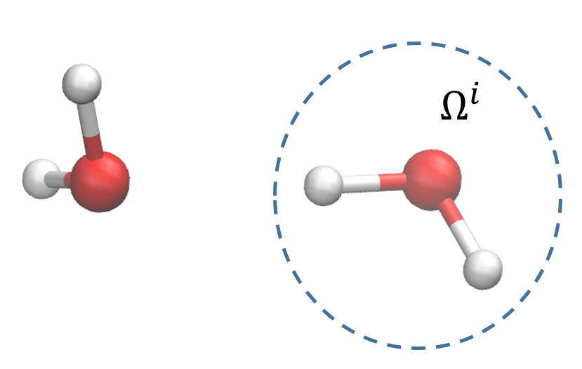
5.1. Water dimer
Our first example is a water dimer system (Fig. 3). The system is partitioned into two parts, with one water molecule described as and the other molecule as . Here poles are used in the PEXSI and PEXSI- method to guarantee accuracy. At the equilibrium configuration, the total energy obtained from the DIAG method is au, and the total energy obtained from the PEXSI method is au, with discrepancy less than au. Therefore the results from DIAG and PEXSI fully agree with each other.
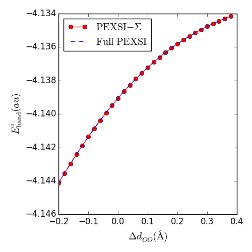
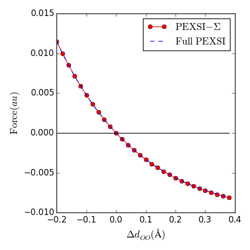
In order to demonstrate that the PEXSI- method gives accurate results in different atomic configurations, we stretch the water molecule in along the oxygen-oxygen direction, and denote by the displacement away from equilibrium position. In the PEXSI- method, the value of the Hamiltonian matrix elements between and vary with respect to the change of the atomic configuration. Hence in the absence of the energy contribution from , the total energies obtained from PEXSI and PEXSI- in general do not agree with each other. However, as discussed in section 4.1, the interior band energy , together with the atomic force corresponding to atoms in should agree well between PEXSI and PEXSI- .
Fig. 3 (a), (b) report the interior band energy, as well as the force on the oxygen atom in projected along the O-O direction, respectively. We find that energies and forces vary smoothly with respect to the change of the O-O distance, and the results from PEXSI and PEXSI- fully agree with each other. We remark that due to the small system size, the exterior degrees of freedom coincide with the boundary degrees of freedom . Hence all matrices are zero. In this special case, the PEXSI- method and the vacuum boundary conditionmethod are the same.
5.2. Divacancy in graphene
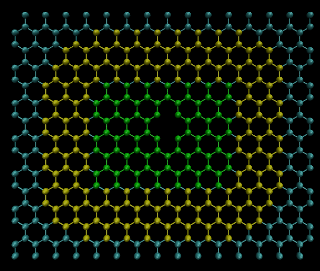
Our second numerical example is a graphene system with a single divacancy defect. Starting from a periodic configuration with atoms, two atoms are removed to create a divacancy (Fig. 5). No further structural relaxation is performed at this stage. In the periodic configuration without the defect, the total energy computed from the DIAG method is au, and the total energy computed from the PEXSI method with poles and at the same chemical potential is au. Hence the results from DIAG and PEXSI fully agree with each other, and all numerical results below will be benchmarked with that from the PEXSI method.
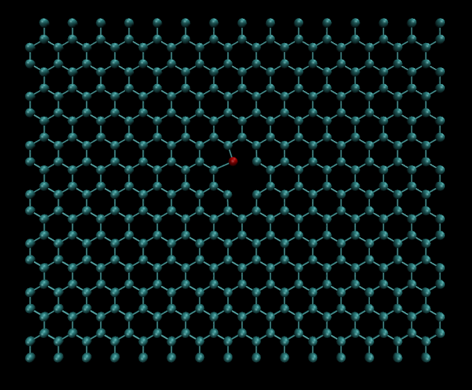
For the divacancy system, the atoms are partitioned according to Fig. 5. Since is non-empty, the matrices are non-zero. In the PEXSI- method, the matrices are obtained from the PEXSI calculation in the periodic configuration. We compare the interior band energy between the divacancy (D) and periodic configuration (P) in Table 1, obtained from PEXSI for the full system, as well as from PEXSI- , and vacuum boundary conditionmethods, respectively. In order to assess the relative accuracy of the methods, we also compare the interior band energy for another system by shifting one atom in Fig. 5 by a small distance of Å along the -direction. The resulting configuration is denoted by SD (shifted divacancy, Fig. 6).
Table 1 indicates that in the periodic configuration, the result from PEXSI- fully agrees with that from the simulation of the full system with PEXSI. Even though the matrix is obtained from the periodic configuration, the inclusion of matrices in the PEXSI- formulation significantly improves the accuracy in other atomic configurations as well. The error of the energy difference between the divacancy and periodic configuration using the vacuum boundary conditionmethod is au. This error is reduced by times to au in the PEXSI- method. Similarly the error of the energy difference between the divacancy and the shifted divacancy configuration using the vacuum boundary conditionmethod is au, and the error is reduced by about times to au in the PEXSI- method.
We report the maximum of the error of the atomic forces calculated from all interior atoms in Table 2. In all configurations, the maximum force error obtained from the PEXSI- method is less than au, which is very accurate for geometry optimization and molecular dynamics studies. Compared to the vacuum boundary conditionmethod, the improvement due to the inclusion of the matrix is again nearly 2 orders of magnitude.
| System | Full PEXSI | PEXSI- | Vacuum |
|---|---|---|---|
| Periodic (P) | -145.70244 | -145.70244 | -145.76624 |
| Divacancy (D) | -142.56345 | -142.56367 | -142.61273 |
| Shifted Divacancy (SD) | -142.45347 | -142.45368 | -142.50003 |
| Energy difference (D-P) | 3.13899 | 3.13877 | 3.15351 |
| Energy difference (SD-D) | 0.10999 | 0.11003 | 0.11270 |
| System | PEXSI- | Vacuum |
|---|---|---|
| Periodic (P) | 0.00000 | 0.00407 |
| Divacancy (D) | 0.00003 | 0.00399 |
| Shifted Divacancy (SD) | 0.00003 | 0.00384 |
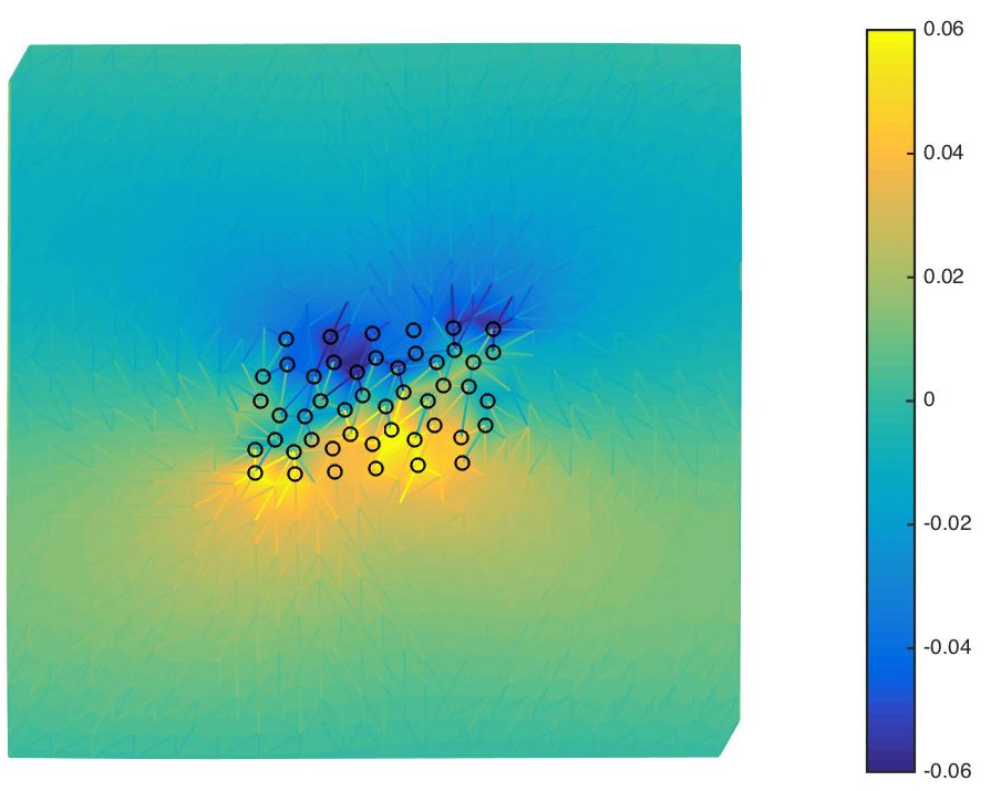
5.3. Dislocation dipole in graphene
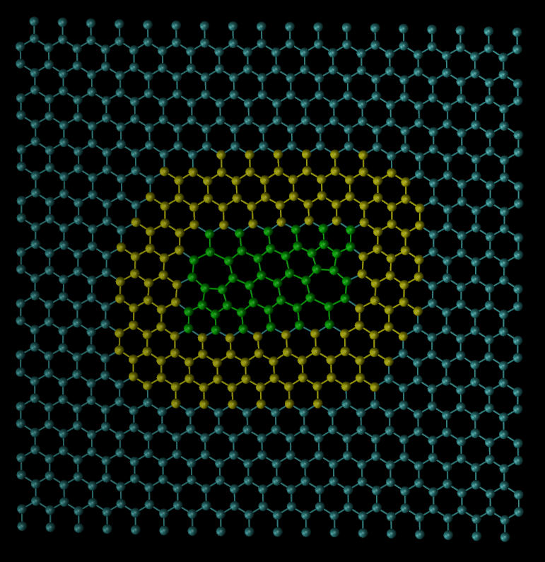
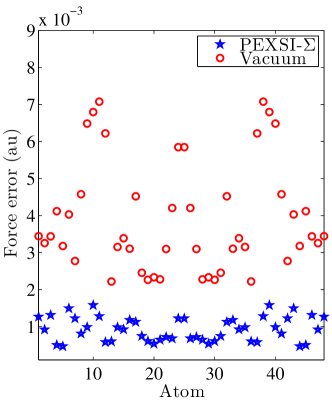
In this test problem, we consider a dislocation dipole in the graphene system. Such a dislocation can be identified as a pentagon-heptagon (5-7) pairs among the hexagonal rings [bonilla2012driving]. As comparison, we form a supercell with 720 atoms in total. The entire system is 4.55nm4.38nm. The lattice constant is set to Å. For the force constant matrix , we performed a calculation in DFTB+ using a supercell with 48 atoms. The matrix is then produced by DFTB as the Hessian matrix. Based on the magnitude of each block, which corresponds to the interaction of an atom with its neighbors, we make a truncation. In particular, the diagonal block has norm ( norm) about au. We keep the force constants from up to 6th neighbors. The distance is about where the norm of the force constant matrix has been reduced to about au. Fig. 7 (a) shows the atomic configuration as well as the partition of the system. We observe that the cut-off of the atoms interactions is slightly smaller than that of the QM model. Compared to the example in section 5.2, the interior domain is reduced to be just around the dislocation dipole. Structural relaxation is also performed for the entire system so that all atoms, including the atoms in the exterior domain, deviate from the equilibrium position, as shown in Fig. 7 (b). The matrix is still constructed from the graphene system with periodic structure. Fig. 8 shows that even with a small interior domain and deformed atomic configuration in the exterior domain, the accuracy of PEXSI- reduces the error of the force uniformly for all atoms in the interior domain to be around au.
6. Conclusion and future work
In this work we proposed a new Green’s function embedding method called PEXSI- for efficient treatment of boundary conditions in complex materials. The matrices can be constructed using Green’s functions corresponding to any physical reference system that shares a similar potential corresponding to exterior degrees of freedom. The matrices can be viewed as a surface potential and do not introduce additional interaction among the interior degrees of freedom. Hence for systems with large number of interior degrees of freedom, the calculation can be performed efficiently using the pole expansion and selected inversion method (PEXSI). Numerical results using non-self-consistent DFTB+ calculations for water dimer, graphene with divacancy and graphene with dislocation dipole demonstrated the accuracy of the method.
We note that our current implementation of the PEXSI- method, which is only serial, is just a proof of principle. As indicated by the performance of the PEXSI method [LinGarciaHuhsEtAl2014, JacquelinLinYang2015], when the number of interior degrees of freedom is large, the PEXSI- method should readily allow a massively parallel implementation in the future with at most complexity. In order to apply the PEXSI- method for the accurate computation of physical quantities, we need to include the self-consistent field effect, which requires the solution of a Coulomb-like equation on the global domain. In particular, the electrostatic energy depends sensitively on the total number of electrons in the system. It is most natural to use a fixed chemical potential. This corresponds to the grand canonical ensemble in the PEXSI- method, and may be a more natural choice for describing processes with charge transfer. However, the grand canonical ensemble treatment might need to be relaxed when the reference system is of finite size. The matrices are constructed from , which is only exact in the absence of deformation of exterior degrees of freedom. When the potential in the exterior domain changes due to atomic relaxation or long range Coulomb interaction, the correction to the matrix could be possibly computed by means of perturbation theory. We also remark that Green’s function embedding methods may also become more versatile if the matrices exhibit certain locality properties to accommodate structural changes of atoms in the exterior domain such as in the presence of a single dislocation, and also can be used to study interaction of defects by using multiple disconnected QM regions. Green’s function embedding methods may also be an attractive alternative for coupling with electronic structure theories beyond the level of KSDFT (see e.g., the recent works [ZgidChan2011, NguyenKananenkaZgid2016, ChibaniRenSchefflerEtAl2016]). We plan to explore these directions in the future.