On the orthogonality of the Chebyshev-Frolov lattice and applications

Abstract

We deal with lattices that are generated by the Vandermonde matrices associated to the roots of Chebyshev-polynomials. If the dimension $d$ of the lattice is a power of two, i.e. $d=2^{m},m\in\mathbb{N}$, the resulting lattice is an admissible lattice in the sense of Skriganov [12]. These are related to the Frolov cubature formulas, which recently drew attention due to their optimal convergence rates [18] in a broad range of Besov-Lizorkin-Triebel spaces. We prove that the resulting lattices are orthogonal and possess a lattice representation matrix with entries not larger than $2$ (in modulus). This allows for an efficient enumeration of the Frolov cubature nodes in the $d$-cube $[-1/2,1/2]^{d}$ up to dimension $d=16$.

1 Introduction

A lattice is a set of points in ${\mathbb{R}}^{d}$ given by

$$\Gamma_{A}=A({\mathbb{Z}^{d}})=\Big{\{}\sum_{j=1}^{d}k_{j}a_{j}:(k_{1},\ldots,k_{d})\in{\mathbb{Z}^{d}}\Big{\}}\,,$$

where the $a_{j}\in{\mathbb{R}}^{d}$ are the columns of the generating matrix $A\in\mathbb{R}^{d\times d}$. Of particular interest are admissible lattices $\Gamma$ in the sense of Skriganov [12] which fulfill

$$\inf\limits_{\gamma\in\Gamma\setminus\{0\}}\Big{|}\prod\limits_{i=1}^{d}\gamma_{i}\Big{|}>0\,.$$ (1.1)

This immediately implies that any vector in the lattice (except the zero vector) consists of only non-vanishing components. However, the condition in (1.1) is much stronger than that and crucial for the performance of the Frolov [6] cubature formula for multivariate functions with ${\rm supp\,}f\subset[-1/2,1/2]^{d}$ given by

$$\Phi(n,A;f):=\frac{1}{n}\sum\limits_{k\in{\mathbb{Z}^{d}}}f\left((n\det(A))^{-1/d}Ak\right)\,,\quad n\in\mathbb{N}\,,$$ (1.2)

see also Bykovskii [2], Dubinin [3, 4], Temlyakov [14, 15] and the recent papers by M. Ullrich [16, 17], Nguyen, M. Ullrich and T. Ullrich [18, 11] and Krieg, Novak [8]. Its asymptotic performance is well-understood as it provides optimal convergence rates for several classes of functions with bounded mixed derivative and compact support, given that $\Gamma_{A}=A({\mathbb{Z}^{d}})$ is admissible.

However, there is a degree of freedom in choosing the lattice generating matrix $A$ in (1.2) such that property (1.1) holds which significantly affects the numerical properties of the algorithm. In the original paper by Frolov [6] a Vandermonde matrix

$$A=\left(\begin{array}[]{cccc}1&\xi_{1}&\cdots&\xi_{1}^{d-1}\\ 1&\xi_{2}&\cdots&\xi_{2}^{d-1}\\ \vdots&\vdots&\ddots&\vdots\\ 1&\xi_{d}&\cdots&\xi_{d}^{d-1}\end{array}\right)\,$$ (1.3)

has been considered, where $\xi_{1},\ldots,\xi_{d}$ are the real roots of an irreducible polynomial over $\mathbb{Q}$, e.g., $P_{d}(x):=\prod_{j=1}^{d}(x-2j+1)-1$ . The general principle of this construction has been elaborated in detail by Temlyakov in his book [14, IV.4] based on results on algebraic number theory, see Borevich, Shafarevich [1] or Gruber, Lekkerkerker [7].

The above polynomial $P_{d}$ has a striking disadvantage, namely that the real roots of the polynomials grow with $d$ and therefore the entries in $A$ get huge due to the Vandermonde structure. In fact, sticking to the structure (1.3), it seems to be a crucial task to find proper irreducible polynomials with real roots of small modulus. In [14, IV.4] Temlyakov proposed the use of rescaled Chebyshev polynomials $Q_{d}$. To be more precise we use for $x\in[-2,2]$

$$Q_{d}(x)=2T_{d}(x/2)\quad\mbox{with}\quad T_{d}(\cdot):=\cos(d\arccos(\cdot))\,.$$ (1.4)

The polynomials $Q_{d}$ belong to $\mathbb{\mathbb{Z}}[x]$ and have leading coefficient $1$. Its roots are real and given by

$$\xi_{k}=2\cos\Big{(}\frac{\pi(2k-1)}{2d}\Big{)}\quad,\quad k=1,...,d\,.$$ (1.5)

In the sequel we will denote the Vandermonde matrix (1.3) with the scaled Chebyshev roots (1.5) by the letter $T$ and call the corresponding lattice $\Gamma_{T}=T({\mathbb{Z}^{d}})$ a Chebyshev lattice. Our main result reads as follows.

Theorem 1.1.

The $d$-dimensional Chebyshev lattice $\Gamma_{T}=T({\mathbb{Z}^{d}})$ is orthogonal. In particular, there exists a lattice representation $\tilde{T}=TS$ with $S\in\text{SL}_{d}(\mathbb{Z})$ such that

• $\tilde{T}_{k,\ell}\in[-2,2]$ for $k,\ell=1,...,d$ and

• $\tilde{T}^{\top}\tilde{T}=\mathrm{diag}(d,2d,\ldots,2d)$.

However, Chebyshev-polynomials are not always irreducible over $\mathbb{Q}$. In fact, the polynomials $Q_{d}$ are irreducible if and only if $d=2^{m}$ [14, IV.4]. Hence, a Chebyshev lattice $\Gamma_{T}$ is admissible if and only if $d=2^{m}$. In that case we call $\Gamma_{T}$ a Chebyshev-Frolov lattice and obtain the following corollary.

Corollary 1.2.

If $d=2^{m}$ for some $m\in\mathbb{N}$ the Chebyshev-Frolov lattice $\Gamma_{T}=T({\mathbb{Z}^{d}})$ and its dual lattice are both orthogonal and admissible. In particular, there is a lattice representation for $\Gamma$ given by $\tilde{T}=QD$ with a diagonal matrix $D=\mathrm{diag}(\sqrt{d},\sqrt{2d},...,\sqrt{2d})$ and an orthogonal matrix $Q$. For the dual lattice $\Gamma^{\perp}$ we have the representation $\tilde{T}^{\perp}=QD^{-1}$.

This observation significantly affects the runtime of an algorithm enumerating the lattice points belonging to $[-1/2,1/2]^{d}$ which represents a first non-trivial step in the implementation of the Frolov cubature formula, see Section 4, 5. By heavily relying on the orthogonality of the respective Chebyshev lattice we give an upper bound in Section 5 for the number of points which have to be seen in order to enumerate the $N$ lattice points in the $d$-cube $[-1/2,1/2]^{d}$. We confirm the result with some numerical tests up to dimension $d=16$. It turns out that we do not have to touch more than $2.07^{d}\cdot N$ points of the lattice.

Let us finally refer to a forthcoming paper by M. Ullrich and the authors for the implementation and comparison of the performance of Frolov’s method to other up to date cubature formulas. There we will also pay special attention to the case $d\neq 2^{m}$.

Notation. As usual $\mathbb{N}$ denotes the natural numbers, $\mathbb{Z}$ denotes the integers, and $\mathbb{R}$ the real numbers . The letter $d$ is always reserved for the underlying dimension in ${\mathbb{R}}^{d},{\mathbb{Z}^{d}}$ etc. We denote with $(x,y)$ the usual Euclidean inner product in ${\mathbb{R}}^{d}$. For $0<p\leq\infty$ we denote with $|\cdot|_{p}$ and $\|\cdot\|_{p}$ the ($d$-dimensional) discrete $\ell_{p}$-norm and the continuous $L_{p}$-norm on ${\mathbb{R}}^{d}$, respectively, where $B_{p}^{d}$ denotes the respective unit ball in $\mathbb{R}^{d}$. With $\mathcal{F}$ we denote the Fourier transform given by $\mathcal{F}f(\xi):=(2\pi)^{-d/2}\int_{{\mathbb{R}}^{d}}f(x)\exp(-ix\cdot\xi)\,\mathrm{d}x$ for a function $f\in L_{1}({\mathbb{R}}^{d})$ and $\xi\in{\mathbb{R}}^{d}$. For two sequences of real numbers $a_{n}$ and $b_{n}$ we will write $a_{n}\lesssim b_{n}$ if there exists a constant $c>0$ such that $a_{n}\leq c\,b_{n}$ for all $n$. We will write $a_{n}\asymp b_{n}$ if $a_{n}\lesssim b_{n}$ and $b_{n}\lesssim a_{n}$. With $\mathrm{GL}_{d}:=\mathrm{GL}_{d}(\mathbb{R})$ we denote the group of invertible matrices over $\mathbb{R}$, wheras $\mathrm{SO}_{d}:=\mathrm{SO}_{d}(\mathbb{R})$ denotes the group of orthogonal matrices over $\mathbb{R}$ with unit determinant. With $\mathrm{SL}_{d}(\mathbb{Z})$ we denote the group of invertible matrices over $\mathbb{Z}$ with unit determinant. The notation $D:=\mbox{diag}(x_{1},...,x_{d})$ with $x=(x_{1},...,x_{d})\in{\mathbb{R}}^{d}$ refers to the diagonal matrix $D\in\mathbb{R}^{d\times d}$ with $x$ at the diagonal. And finally, by $\mathbb{Z}[x]$ we denote the ring of polynomials with integer coefficients.

2 Construction of admissible lattices

In this section we will briefly recall the precise notions of a lattice, its dual lattice, orthogonal and admissible lattices. We will furthermore comment on different lattice representations.

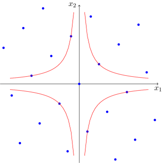
Figure 1: Admissible lattice and hyperbolic cross.

Definition 2.1 (Lattice).

A (full-rank) lattice $\Gamma\subset{\mathbb{R}}^{d}$ is a subgroup of ${\mathbb{R}}^{d}$ which is isomorphic to ${\mathbb{Z}^{d}}$ and spans the real vector space ${\mathbb{R}}^{d}$. A set $\{a_{1},...,a_{d}\}\subset\Gamma$ such that $\mbox{\rm span}_{\mathbb{Z}}\{a_{1},...,a_{d}\}=\Gamma$ is called generating set of $\Gamma$. The matrix $A=(a_{1}|\cdots|a_{d})\in\mbox{\rm GL}_{d}$ is called a generating matrix for $\Gamma$, i.e., we can write

$$\Gamma:=\{Ak:k\in{\mathbb{Z}^{d}}\}\,.$$

Let us further introduce the dual lattice.

Definition 2.2 (Dual lattice).

For a lattice $\Gamma\subset{\mathbb{R}}^{d}$ we define the dual lattice $\Gamma^{\bot}$ as

$$\Gamma^{\bot}=\{x\in{\mathbb{R}}^{d}:(x,y)\in\mathbb{Z}\text{ for all }y\in\Gamma\}\,.$$

If $A$ is a generating matrix for $\Gamma$ then $A^{-\top}$ is a generating matrix for $\Gamma^{\bot}$.

Crucial for the performance of the Frolov cubature formula (1.2) will be the notion of “admissibility” which is settled in the following definition.

Definition 2.3 (Admissible lattice).

A lattice $\Gamma$ is called admissible if

$$\mathrm{Nm}(\Gamma):=\inf_{\gamma\in\Gamma\setminus\{0\}}\Big{|}\prod_{i=1}^{d}\gamma_{i}\Big{|}>0$$

holds true.

Figure 1 illustrates this property. In fact, lattice points different from $0$ lie outside of a hyperbolic cross with “radius” $\mathrm{Nm}(\Gamma)$.

The following lemma is essentially [12, Lem. 3.1/2]. In the special case of a Vandermonde generator (1.3) we refer to [18, Lem. 2.1].

Lemma 2.4.

If a lattice $\Gamma\subset{\mathbb{R}}^{d}$ is admissible then $\Gamma^{\bot}\subset{\mathbb{R}}^{d}$ is also admissible.

There is a generic way to construct an admissible lattice described in Temlyakov [14, IV.4]. For a polynomial $P(x)\in\mathbb{Z}[x]$ of order $d$ which is irreducible over $\mathbb{Q}$ and has $d$ different real roots $\xi_{1},\xi_{2},\ldots,\xi_{d}$ one can define the Vandermonde matrix $A=(a_{kl})_{k,l=1}^{d}=(\xi_{k}^{l-1})_{k,l=1}^{d}$, see (1.3) above, which generates an admissible lattice $\Gamma$ with $\mathrm{Nm}(\Gamma)=1$. We will call such a generating matrix Frolov matrix since this construction has been already used by Frolov [6]. Frolov originally used the construction to define the matrix $B$ which generates the dual lattice, and then $A=B^{-\top}$ was chosen as the lattice generator in the Frolov cubature formula. The reason is that convergence properties of the method require admissibility of the dual lattice. However, in [12, Lem. 3.1] Skriganov has shown (see Lemma 2.4 above) that if $B$ generates an admissible lattice, so does $A$, which means that both $B$ and $A$ are valid matrices for the Frolov cubature formula. A Frolov matrix with a small determinant is desirable since the Frolov cubature formula using this matrix will show (relatively) good preasymptotic behavior. The determinant of $A=(a_{kl})_{k,l=1}^{d}=(\xi_{k}^{l-1})_{k,l=1}^{d}$ is given by

$$\det(A)=\prod_{k\neq l}(\xi_{k}-\xi_{l})\,.$$

Therefore we need polynomials $P$ which additionally have accumulated roots. To find such polynomials is a challenging task, however, for certain dimensions there are results available which will be given in Section 3.

Let us now consider different representations of a given lattice $\Gamma_{A}:=A({\mathbb{Z}^{d}})$ generated by $A\in\mbox{GL}_{d}$. This representation is not unique, because any linear automorphism $S$ on ${\mathbb{Z}^{d}}$ yields $S({\mathbb{Z}^{d}})={\mathbb{Z}^{d}}$ and consequently $AS({\mathbb{Z}^{d}})=A({\mathbb{Z}^{d}})$. This gives rise to the question which lattice representation is favorable from the numerical point of view, cf. Figure 2. In the special case of orthogonal lattices, the orthogonal representation stands out obviously.

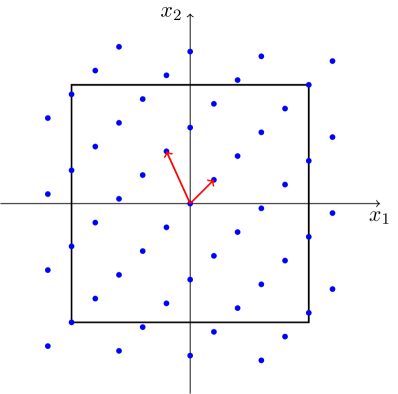
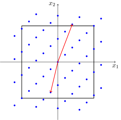
Figure 2: Equivalent lattice representations within the unit cube $\Omega=\left[-1/2,1/2\right]^{2}$.

Definition 2.5 (Orthogonal lattice).

A lattice $\Gamma$ is called orthogonal if there exists a generating matrix $A\in\mbox{\rm GL}_{d}(\mathbb{R})$ which has orthogonal column vectors.

In general, the computation of an orthogonal representation for an orthogonal lattice is performed by a discrete variant of the Gram-Schmidt method, e.g. the Lenstra-Lenstra-Lovász–lattice basis reduction algorithm (LLL), see [10] or its modifications. However, as it turns out, in the case of Chebyshev-lattices an orthogonal basis can be determined a priori without any additional computational effort as we will show in the following Section.

3 Orthogonality of Chebyshev lattices

Let $d\in\mathbb{N}$ and consider the Vandermonde matrix $T=(\xi_{k}^{l-1})_{k,l=1}^{d}$, where

$$\xi_{k}=2\cos\left(\pi\frac{2k-1}{2d}\right)\quad,\quad k=1,\ldots,d\,,$$

represent the roots of $Q_{d}(x)=2T_{d}(\frac{x}{2})\in\mathbb{Z}[x]$ and $T_{d}$ denotes the $d$-th Chebyshev polynomial. The lattice $\Gamma_{T}=T({\mathbb{Z}^{d}})$ will be called Chebyshev lattice, and it is admissible if and only if $d=2^{m}$, see [14], in which case we will call it Chebyshev-Frolov lattice. In fact, it is easy to show that for $d\neq 2^{m}$ the polynomial $Q_{d}(x)$ has a divisor which itself is a scaled Chebyshev polynomial $Q_{d^{\prime}}(x)$ of lower order $d^{\prime}=2^{m^{\prime}}$ for some $m^{\prime}\in\mathbb{N}$.

Our main result reads as follows.

Theorem 3.1.

The Chebyshev lattice $\Gamma_{T}=T(\mathbb{Z}^{d})$ is an orthogonal lattice.

To show this, we will derive a lattice representation matrix $\tilde{T}=TS$, $S\in\mbox{SL}_{d}(\mathbb{Z})$ and show that it has orthogonal column vectors.

Lemma 3.2.

For $\omega\in\mathbb{R}$ and $l\in\mathbb{N}$ define $\eta_{l}=2\cos(l\omega\pi)$. Then

$$\eta_{1}^{l}-\eta_{l}\in\mathbb{Z}[\eta_{1},\dots,\eta_{l-1}]\quad,\quad l\in\mathbb{N}.$$

More precisely, there exist integers $m^{(l)}_{j}\in\mathbb{Z}$ independent of $\omega$ such that for any $l\in\mathbb{N}$

$$\eta_{1}^{l}-\eta_{l}=m_{0}+\sum_{j=1}^{l-1}m^{(l)}_{j}\eta_{j}\,.$$

Proof.

The proof is a straightforward calculation using Euler’s formula by putting

$$\eta_{1}^{l}-\eta_{l} = \left(e^{\omega\pi\mathrm{i}}+e^{-\omega\pi\mathrm{i}}\right)^{l}-\left(e^{\omega\pi\mathrm{i}l}+e^{-\omega\pi\mathrm{i}l}\right)$$

$$= \displaystyle\sum_{j=0}^{l}\binom{l}{j}e^{\omega\pi\mathrm{i}(l-2j)}-\left(e^{\omega\pi\mathrm{i}l}+e^{-\omega\pi\mathrm{i}l}\right)$$

$$= \displaystyle\sum_{j=1}^{l-1}\binom{l}{j}e^{\omega\pi\mathrm{i}(l-2j)}$$

$$= \begin{cases}\displaystyle\sum_{j=1}^{\frac{l-1}{2}}\binom{l}{j}\left(e^{\omega\pi\mathrm{i}(l-2j)}+e^{-\omega\pi\mathrm{i}(l-2j)}\right)&:l\text{ odd}\,,\\ \displaystyle\sum_{j=1}^{\lfloor\frac{l-1}{2}\rfloor}\binom{l}{j}\left(e^{\omega\pi\mathrm{i}(l-2j)}+e^{-\omega\pi\mathrm{i}(l-2j)}\right)+\binom{l}{\frac{l}{2}}e^{\omega\pi\mathrm{i}(l-l)}&:l\text{ even}\end{cases}$$

$$= \begin{cases}\displaystyle\sum_{j=1}^{\frac{l-1}{2}}\binom{l}{j}2\cos(\omega\pi(l-2j))&:l\text{ odd}\,,\\ \displaystyle\sum_{j=1}^{\lfloor\frac{l-1}{2}\rfloor}\binom{l}{j}2\cos(\omega\pi(l-2j))+\binom{l}{\frac{l}{2}}&:l\text{ even}\,.\end{cases}$$

The values $m_{j}^{(l)}$ can be obtained from this representation. ∎

This lemma leads to our desired lattice representation, since multiplying with a matrix $S\in\mbox{SL}_{d}(\mathbb{Z})$ from the right is a composition of column operations.

Corollary 3.3.

The matrix $\tilde{T}=TS$, where $S\in\ \mbox{SL}_{d}(\mathbb{Z})$ is a suitable column operation matrix, given by

$$\tilde{T}_{kl}=\begin{cases}1&:l=1\,,\\ 2\cos\left(\pi(l-1)\frac{2k-1}{2d}\right)&:l=2\dots d\end{cases}$$

generates the lattice $\Gamma_{T}=T(\mathbb{Z}^{d})$.

Proof.

The case $d=2$ is trivial, so assume $d>2$. For $i=3\dots d$ we define $S^{(l)}\in\mbox{SL}_{d}(\mathbb{Z})$ to be a column operation matrix changing the $l$-th column:

$$S^{(l)}=\left(\begin{array}[]{cccccc}1&&&-m_{0}^{(l)}&&\\ &\ddots&&\vdots&&\\ &&\ddots&-m_{l-2}^{(l)}&&\\ &&&1&&\\ &&&&\ddots&\\ &&&&&1\end{array}\right)\,$$ (3.1)

Then the product matrix $S=S^{(3)}\cdots S^{(d)}$ consecutively transforms the entries of $T$ which have the form $\xi_{k}^{l-1}=2\cos(\pi\frac{2k-1}{2d})^{l-1}$ according to Lemma 3.2. ∎

We remark that this formula is applicable in general to any Vandermonde lattice with generating factors ranging from $-2$ to $2$. Furthermore, $\tilde{T}$ has better stability properties than $T$. The following lemma will complete the proof of Theorem 1.1.

Lemma 3.4.

The matrix $\tilde{T}$ is orthogonal. Moreover, it holds $\tilde{T}^{\top}\tilde{T}=\mathrm{diag}(d,2d,...,2d)$ .

Proof.

For $l=2\dots d$ we have

$$((\tilde{T})^{\top}\tilde{T})_{1l} = \displaystyle\sum_{k=1}^{d}2\cos\left(\pi(l-1)\frac{2k-1}{2d}\right)$$

$$= \displaystyle\sum_{k=1}^{d}\left(e^{\mathrm{i}\pi(l-1)\frac{2k-1}{2d}}+e^{-\mathrm{i}\pi(l-1)\frac{2k-1}{2d}}\right)$$

$$= \displaystyle\sum_{k=1}^{2d}e^{\mathrm{i}\pi(l-1)\frac{2k-1}{2d}}\,.$$

We continue observing

$$\sum_{k=1}^{2d}e^{2\pi\mathrm{i}(l-1)\frac{2k-1}{4d}}=\left(\displaystyle\sum_{k=1}^{2d}e^{2\pi\mathrm{i}(l-1)\frac{k}{2d}}\right)e^{\frac{{-2\pi\mathrm{i}(l-1)}}{4d}}=\frac{1-e^{2\pi\mathrm{i}(l-1)}}{1-e^{2\pi\mathrm{i}\frac{(l-1)}{2d}}}e^{\frac{{-2\pi\mathrm{i}(l-1)}}{4d}}=0\,.$$

Let us now consider $l=2\dots d$ and $j=2\dots d$. We find

$$((\tilde{T})^{\top}\tilde{T})_{jl} = \displaystyle\sum_{k=1}^{d}2\cos\left(\pi(j-1)\frac{2k-1}{2d}\right)2\cos\left(\pi(l-1)\frac{2k-1}{2d}\right)$$

$$= \displaystyle\sum_{k=1}^{d}\left(e^{\pi\mathrm{i}(j-1)\frac{2k-1}{2d}}+e^{-\pi\mathrm{i}(j-1)\frac{2k-1}{2d}}\right)\left(e^{\pi\mathrm{i}(l-1)\frac{2k-1}{2d}}+e^{-\pi\mathrm{i}(l-1)\frac{2k-1}{2d}}\right)$$

$$= \displaystyle\sum_{k=1}^{d}e^{\pi\mathrm{i}(j+l-2)\frac{2k-1}{2d}}+e^{\pi\mathrm{i}(j-l)\frac{2k-1}{2d}}+e^{\pi\mathrm{i}(l-j)\frac{2k-1}{2d}}+e^{-\pi\mathrm{i}(j+l-2)\frac{2k-1}{2d}}$$

$$= \displaystyle\sum_{k=1}^{2d}e^{2\pi\mathrm{i}(j+l-2)\frac{2k-1}{4d}}+\sum_{k=1}^{2d}e^{2\pi\mathrm{i}(j-l)\frac{2k-1}{4d}}=\begin{cases}2d&:j=l\\ 0&:\text{otherwise}\,.\end{cases}$$

∎

4 The Frolov cubature formula

We return to the Frolov cubature formula (1.2) mentioned in the introduction, see [6, 12, 14, 15, 18], to estimate integrals of the form

$$I(f):=\int_{\Omega}f(x)\,\mathrm{d}x\,,$$

where $\Omega\subset{\mathbb{R}}^{d}$ is a compact set. The matrix $T\in\mathbb{R}^{d\times d}$ is chosen such that $T({\mathbb{Z}^{d}})$ is an admissible lattice, for instance the Chebyshev-Frolov matrix from above. For a given scaling parameter $n\in\mathbb{N}$ we define the matrix

$$\mathcal{T}_{n}=(n\det(T))^{-\frac{1}{d}}T,$$ (4.1)

which satisfies $\det(\mathcal{T}_{n})=1/n$. Defining $\Gamma_{n}=\mathcal{T}_{n}(\mathbb{Z}^{d})$, the integration nodes are chosen as the elements of the lattice $\Gamma_{n}$ belonging to $\Omega$, i.e. $N(n):=|\Gamma_{n}\cap\Omega|$. Note, that the cubature weights of the Frolov method are chosen to be uniformly $1/n$. But, despite the uniformity of the weights, the Frolov cubature formula does not represent a Quasi–Monte Carlo method since in general $N(n)\neq n$, i.e., the weights do not sum up to one. However, we have that $\lim_{n\to\infty}\tfrac{|\Gamma_{n}\cap\Omega|}{n}=\mathrm{vol}(\Omega)$.

The formula (1.2) performs asymptotically optimal for a broad variety of function spaces with dominating mixed smoothness, see [18]. To this end, we define the Besov spaces of dominating mixed smoothness as follows.

Definition 4.1 (Besov space of mixed smoothness).

Let $0<p,\theta\leq\infty$, $r>\max\{1/p-1,0\}$, and $(\varphi_{m})_{m\in\mathbb{N}_{0}^{d}}$ be a tensorized decomposition of unity in the sense of [5, Rem. 3.3]. The Besov space of dominating mixed smoothness $\mathbf{B}^{r}_{p,\theta}=\mathbf{B}^{r}_{p,\theta}({\mathbb{R}}^{d})$ is the set of all $f\in L_{1}({\mathbb{R}}^{d})$ such that

$$\|f\|_{\mathbf{B}^{r}_{p,\theta}}\,:=\,\Big{(}\sum_{m\in\mathbb{N}_{0}^{d}}2^{r|m|_{1}\theta}\,\|\mathcal{F}^{-1}[\varphi_{m}\mathcal{F}f]\|_{p}^{\theta}\Big{)}^{1/\theta}\,<\,\infty$$

with the usual modification for $\theta=\infty$.

In the special case $p=\theta=2$ we put $H^{r}_{\text{mix}}({\mathbb{R}}^{d}):=\mathbf{B}^{r}_{p,\theta}$ which denotes the Sobolev spaces of dominating mixed smoothness $r$. Let us restrict to the case $\Omega:=[-1/2,1/2]^{d}$ in the sequel and define a subspace of $\mathbf{B}^{r}_{p,\theta}$, namely the space of $\mathring{\mathbf{B}}_{p,\theta}^{r}$ of functions which are supported in the unit cube $[-1/2,1/2]^{d}$, i.e. we consider

$$\mathring{\mathbf{B}}_{p,\theta}^{r}\,:=\,\bigl{\{}f\in\mathbf{B}^{r}_{p,\theta}({\mathbb{R}}^{d})\colon{\rm supp\,}(f)\subset[-1/2,1/2]^{d}\bigr{\}}\,.$$ (4.2)

In [4, 18] it has been shown in case $1\leq p,\theta\leq\infty$ and $r>1/p$ that

$$\sup\limits_{f\in\mathring{\mathbf{B}}_{p,\theta}^{r},\|f\|_{\mathbf{B}^{r}_{p,\theta}}\leq 1}|I(f)-\Phi(T,n;f)|\asymp n^{-r}(\log n)^{(d-1)(1-1/\theta)}\,,$$ (4.3)

where the constant behind $\asymp$ depends on $d$ and the choice of $T$. Note, that the rate in (4.3) is independent of the integrability parameter $p$. Taking into account that the number $N(n)$ of cubature nodes satisfies

$$N(n):=n+O(\log^{d-1}n)\,,$$ (4.4)

see [12, (0.1)], the rate of convergence (4.3) is optimal among all cubature formulas with $N$ arbitrary nodes and weights.

5 Enumerating the Chebyshev-Frolov nodes

In order to generate the Frolov cubature nodes belonging to $\Omega:=[-1/2,1/2]^{d}$ explicitly one needs an efficient way to enumerate all points from $\Gamma_{n}\cap\Omega$, which already in moderate dimensions is a difficult task. In fact, we need to determine

$$X_{n}:=\mathcal{T}_{n}(\mathbb{Z}^{d})\cap\left[-\frac{1}{2},\frac{1}{2}\right]^{d}$$ (5.1)

as efficient as possible. This is equivalent to finding the pre-image of $[-1/2,1/2]^{d}$ under the linear map $\mathcal{T}_{n}$ intersected with ${\mathbb{Z}^{d}}$, i.e.

$$Y_{n}:=\left(\mathcal{T}_{n}^{-1}\left[-\frac{1}{2},\frac{1}{2}\right]^{d}\right)\cap\mathbb{Z}^{d},$$ (5.2)

since $k\in Y_{n}$ if and only if $\mathcal{T}_{n}k\in X_{n}$. Now it is a natural approach to use a finite set $K_{n}\subset\mathbb{Z}^{d}$ that covers $Y_{n}$, i.e. $Y_{n}\subset K_{n}$, and allows for an efficient enumeration on a computer. Then, one can check for each vector $k\in K_{n}$ wether $\mathcal{T}_{n}k\in X_{n}$.

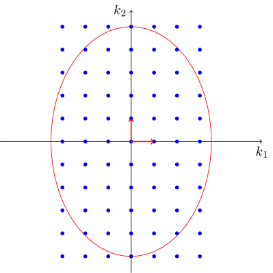
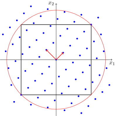
Figure 3: The ellipsoid (left) that is the pre-image under $\mathcal{T}_{n}$ of the bounding ball of $\Omega=[-1/2,1/2]^{2}$ (right).

However, there remains the problem of determining suitable covering sets $K_{n}$. To this end, we note that an efficient enumeration is possible at least for all integer vectors within $\ell_{p}$-ellipsoids that are axis-aligned, i.e.

$$E_{p,d}(R;\mu_{1},\ldots,\mu_{d}):=\Big{\{}x\in\mathbb{R}^{d}:\sum_{j=1}^{d}\Big{|}\frac{x_{j}}{\mu_{j}}\Big{|}^{p}\leq R^{p}\Big{\}},$$ (5.3)

where $R\mu_{1},\ldots,R\mu_{d}>0$ denote the lengthes of the semi-axes. An efficient enumeration of all integer vectors belonging to such a set is possible due to the recursive representation of its discrete counterpart $\mathcal{E}_{p,d}(R;\mu_{1},\ldots,\mu_{d}):=E_{p,d}(R;\mu_{1},\ldots,\mu_{d})\cap{\mathbb{Z}^{d}}$, which reads

$$\mathcal{E}_{p,d}(R;\mu_{1},\ldots,\mu_{d})=\bigcup_{|k_{d}|\leq R\,\mu_{d}}\mathcal{E}_{p,d-1}\left(\left[R^{p}-\left(\frac{|k_{d}|}{\mu_{d}}\right)^{p}\right]^{\frac{1}{p}};\mu_{1},\ldots,\mu_{d-1}\right)\times\{k_{d}\}$$ (5.4)

and can easily be implemented as a $d$-fold nested for-loop. In addition, the cardinality of (5.4), i.e., the number of integer vectors belonging to $E_{p,d}(R;\mu_{1},\ldots,\mu_{d})$ can be estimated following the approach in [9, Sect. 3]. To this end, we have the following result, which relates the number of integer vectors within a general $p$-ellipsoid to its volume. Note at this point the relation $E_{p,d}(R;1,\ldots,1)=R\cdot B_{p}^{d}$, where $B_{p}^{d}$ denotes the unit-ball with respect to the $\ell_{p}$-(quasi)-norm.

Proposition 5.1.

Let $\mu=(\mu_{1},...,\mu_{d})>0$ and $0<p<\infty$.
(i) For the volume of the “unit” ellipsoid $E_{p,d}(1;\mu_{1},\ldots,\mu_{d})$ it holds

$$\mathrm{vol}(E_{p,d}(1;\mu_{1},\ldots,\mu_{d}))=\mathrm{vol}(B_{p}^{d})\prod_{j=1}^{d}\mu_{j}=2^{d}\frac{\Gamma(1+1/p)^{d}}{\Gamma(d/p+1)}\prod_{j=1}^{d}\mu_{j}\,.$$

(ii) If $R>r(\mu,p)$ then the number of integer points in $E_{p,d}(R;\mu_{1},\ldots,\mu_{d})$ is bounded from above and below by

$$\left(R^{\varrho}-r(\mu,p)^{\varrho}\right)^{d/\varrho}\mathrm{vol}(E_{p,d}(1;\mu_{1},\ldots,\mu_{d}))\leq|\mathcal{E}_{p,d}(R;\mu)|\leq\left(R^{\varrho}+r(\mu,p)^{\varrho}\right)^{d/\varrho}\mathrm{vol}(E_{p,d}(1;\mu_{1},\ldots,\mu_{d}))\,,$$

where $r(\mu,p):=1/2\,\left(\sum_{j=1}^{d}|\mu_{j}|^{-p}\right)^{1/p}$ and $\varrho:=\min\{p,1\}$.
(iii) It holds

$$\lim\limits_{R\to\infty}\frac{|\mathcal{E}_{p,d}(R;\mu)|}{R^{d}}=\mathrm{vol}(E_{p,d}(1;\mu_{1},\ldots,\mu_{d}))\,.$$

Proof.

The formula in (i) is obtained by change of variable and the well-known formula for the volume of standard $\ell_{p}$-balls in $\mathbb{R}^{d}$. In fact, we have

$$\int\limits_{\{x\in\mathbb{R}^{d}~{}:~{}\sum_{i}|x_{i}/\mu_{i}|^{p}\leq 1\}}1\,\mathrm{d}x=\Big{(}\prod\limits_{j=1}^{d}\mu_{j}\Big{)}\int\limits_{|y|_{p}\leq 1}1\,dy=2^{d}\frac{\Gamma(1+1/p)^{d}}{\Gamma(d/p+1)}\prod\limits_{j=1}^{d}\mu_{j}\,.$$

The limit statement in (iii) is a direct consequence of (ii).

It remains to prove (ii). Here we use the arguments in [9, Sect. 3] and define a (quasi-)norm on $\mathbb{R}^{d}$ via

$$\|x\|:=\Big{(}\sum\limits_{i=1}^{d}|x_{i}/\mu_{i}|^{p}\Big{)}^{1/p}\quad,\quad x\in\mathbb{R}^{d}\,.$$

Note, that the classical triangle inequality is replaced by the $\varrho$-triangle inequality, where $\varrho:=\min\{1,p\}$, i.e., $\|x+y\|^{\varrho}\leq\|x\|^{\varrho}+\|y\|^{\varrho}$ for all $x,y\in\mathbb{R}^{d}$ . We denote with $B_{\|\cdot\|}$ the (closed) unit ball of $(\mathbb{R}^{d},\|\cdot\|)$. By putting $Q_{k}:=k+[-1/2,1/2]^{d}$ for $k\in\mathbb{Z}^{d}$ we observe according to [9, Sect. 3] as a consequence of the $\varrho$-triangle inequality

$$\ell(R,p,d)B_{\|\cdot\|}\subset\bigcup\limits_{\|k\|\leq R}Q_{k}\subset L(R,p,d)B_{\|\cdot\|}\,,$$

where $\ell(R,p,d):=(R^{\varrho}-r(\mu,p)^{\varrho})^{1/\varrho}$ and $L(R,p,d):=(R^{\varrho}+r(\mu,p)^{\varrho})^{1/\varrho}$ with $r(\mu,p)=\|\sum_{i=1}^{d}e_{i}\|/2$ . Taking volumes on both sides yields (ii). ∎

Now we are in the position to exploit the orthogonality of the Chebyshev-Frolov lattice by choosing a proper bounding ellipsoid with respect to the Euclidian norm, i.e., $p=2$. To this end, we write $\mathcal{T}_{n}=(n\det(D))^{-\frac{1}{d}}QD$ as the scaled product of an orthogonal matrix with unit determinant $Q\in\mathrm{SO}_{d}$ and a diagonal matrix $D=\mbox{diag}(\lambda_{1},...,\lambda_{d})$ with entries

$$\lambda_{1}=\sqrt{d}\quad\mbox{and}\quad\lambda_{2}=\ldots=\lambda_{d}=\sqrt{2d}\,.$$ (5.5)

We note that it holds $[-1/2,1/2]^{d}\subset E_{2,d}(\sqrt{d}/2;1,\ldots,1)=(\sqrt{d}/2)B_{2}^{d}$, the isotropic ball in ${\mathbb{R}}^{d}$ of radius $\sqrt{d}/2$. Therefore we can compute

$$\mathcal{T}_{n}^{-1}[-1/2,1/2]^{d} \subset\mathcal{T}_{n}^{-1}E_{2,d}(\sqrt{d}/2;1,\ldots,1)$$

$$=(n\det(D))^{\frac{1}{d}}D^{-1}Q^{T}E_{2,d}(\sqrt{d}/2;1,\ldots,1)$$

$$=(n\det(D))^{\frac{1}{d}}D^{-1}E_{2,d}(\sqrt{d}/2;1,\ldots,1)$$

$$=E_{2,d}\left(R_{n};\lambda_{1}^{-1},\ldots,\lambda_{d}^{-1}\right),$$

where $R_{n}=\frac{\sqrt{d}}{2}(n\det(D))^{\frac{1}{d}}=\frac{\sqrt{d}}{2}n^{1/d}\prod_{j=1}^{d}\lambda_{j}^{1/d}$. The discrete $\ell_{2}$-ellipsoid

$$K_{n}:=\mathcal{E}_{2,d}(R_{n};\lambda_{1}^{-1},\ldots,\lambda_{d}^{-1}):=E_{2,d}\left(R_{n};\lambda_{1}^{-1},\ldots,\lambda_{d}^{-1}\right)\cap{\mathbb{Z}^{d}}$$ (5.6)

is our desired, easily accessible finite set that covers the pre-image of $X_{n}$. In order to determine the complexity of our enumeration algorithm, we have to bound the cardinality $|K_{n}|$ of $K_{n}$. As a special case of Proposition 5.1 we obtain the following result on this cardinality.

Theorem 5.2.

Let $K_{n}$, $X_{n}$ be given by (5.6), (5.5) and (5.1).
(i) If $n>2^{3d/2}$ then the cardinality $|K_{n}|$ is bounded from below and above by

$$n\Big{(}1-\frac{2^{3/2}}{n^{1/d}}\Big{)}^{d}\frac{(d\pi)^{d/2}}{2^{d}\Gamma(d/2+1)}\quad\leq\quad|K_{n}|\quad\leq\quad n\,\Big{(}1+\frac{2^{3/2}}{n^{1/d}}\Big{)}^{d}\frac{(d\pi)^{d/2}}{2^{d}\Gamma(d/2+1)}\,.$$ (5.7)

(ii) As a consequence, we obtain the limit statements

$$\lim\limits_{n\to\infty}|K_{n}|/n=\lim\limits_{n\to\infty}|K_{n}|/|X_{n}|=\mathrm{vol}((\sqrt{d}/2)B_{2}^{d})\leq\Big{(}\frac{\pi e}{2}\Big{)}^{d/2}\,.$$ (5.8)

Proof.

We apply Proposition 5.1 with $p=2$, $\mu_{1}=d^{-1/2}$, $\mu_{2}=...=\mu_{d}=(2d)^{-1/2}$ and $R_{n}=(\sqrt{d}/2)n^{1/d}\prod_{j=1}^{d}\mu_{j}^{-1/d}$ for $n\in\mathbb{N}$. Due to $\Gamma(3/2)=\sqrt{\pi}/2$ we obtain from Proposition 5.1

$$\frac{\pi^{d/2}}{\Gamma(d/2+1)}\prod\limits_{j=1}^{d}\mu_{j}=\lim\limits_{n\to\infty}\frac{|\mathcal{E}_{2,d}(R_{n};\mu)|}{R_{n}^{d}}=\Big{(}\prod\limits_{j=1}^{d}\mu_{j}\Big{)}(\sqrt{d}/2)^{-d}\lim\limits_{n\to\infty}|K_{n}|/n\,,$$

which immediately implies the second identity in (5.8). Due to $|X_{n}|=N(n)=n+O((\log n)^{d-1})$, see (4.4) above, we obtain the first identity. The inequality is a consequence of $\Gamma(1+x)\geq(x/e)^{x}$.

It remains to prove (5.7). By Proposition 5.1, (ii), we have ($\varrho=1$)

$$(R_{n}-r(\mu,2))^{d}\frac{\pi^{d/2}}{\Gamma(d/2+1)}\prod_{j=1}^{d}\mu_{j}\leq|K_{n}|\leq(R_{n}+r(\mu,2))^{d}\frac{\pi^{d/2}}{\Gamma(d/2+1)}\prod_{j=1}^{d}\mu_{j}\,.$$ (5.9)

By the definition of the $R_{n}$ we have $R_{n}\prod_{j=1}^{d}\mu_{j}^{1/d}=n^{1/d}\sqrt{d}/2$ . Moreover, the special choice of the $\mu_{j}$’s gives

$$r(\mu,2)\prod_{j=1}^{d}\mu_{j}^{1/d}=2^{-\frac{d-1}{2d}}\cdot\sqrt{2d^{2}-d}\frac{1}{\sqrt{d}}\leq\sqrt{2d}\,.$$

Plugging this into (5.9) yields (5.7).∎

One can see, that the cardinality $|K_{n}|$ scales linear in $n$, where the factor depends exponentially on the dimension $d$. The true number of discrete lattice points in $K_{n}$ that have to be “seen” is given in Table 1 for dimensions $d=2,4,8,16$. The relative overhead $|K_{n}||X_{n}|^{-1}$ converges to a constant smaller than $2.07^{d}$ for $n$ tending to infinity, which outlines the complexity of the enumeration algorithm with respect to $N$, where $N=N(n)=|X_{n}|$.

Appendix

Dimension $d=2$
scaling factor $n$	cubature points in $X_{n}$	ellipsoid points $|K_{n}|$	relative overhead $|K_{n}||X_{n}|^{-1}$
64	65	101	1.55
256	257	409	1.59
1024	1027	1599	1.56
4096	4095	6427	1.57
16384	16383	25735	1.57
65536	65539	102951	1.57
262144	262145	411813	1.57
1048576	1048579	1647103	1.57

Dimension $d=4$
scaling factor $n$	cubature points in $X_{n}$	ellipsoid points $|K_{n}|$	relative overhead $|K_{n}||X_{n}|^{-1}$
64	71	347	4.89
256	261	1205	4.62
1024	1025	5061	4.94
4096	4099	20287	4.95
16384	16385	81105	4.95
65536	65533	324241	4.95
262144	262143	1297123	4.95
1048576	1048609	5176701	4.95

Dimension $d=8$
scaling factor $n$	cubature points in $X_{n}$	ellipsoid points $|K_{n}|$	relative overhead $|K_{n}||X_{n}|^{-1}$
64	79	4459	56.44
256	271	15395	56.81
1024	1067	63299	59.32
4096	4113	267005	64.92
16384	16413	1077433	65.65
65536	65645	4231533	64.46
262144	262263	16729291	63.79
1048576	1048779	68078523	64.91

Dimension $d=16$
scaling factor $n$	cubature points in $X_{n}$	ellipsoid points $|K_{n}|$	relative overhead $|K_{n}||X_{n}|^{-1}$
64	423	751915	1777.58
256	967	4349507	4497.94
1024	2043	17758079	8692.16
4096	5835	58780787	10073.83
16384	18901	232153093	12282.58
65536	69353	969855677	13984.34
262144	267257	4086738257	15291.42
1048576	1054837	16642145301	15776.98

Table 1: Cardinalities of the sets of Frolov-cubature points $X_{n}$, the bounding ellipsoids $K_{n}$ and the relative overhead.

References

• [1] A.ย I. Borevich and I.ย R. Shafarevich. Number theory. Translated from the Russian by Newcomb Greenleaf. Pure and Applied Mathematics, Vol. 20. Academic Press, New York-London, 1966.
• [2] V.ย Bykovskii. On the correct order of the error of optimal cubature formulas in spaces with dominant derivative, and on quadratic deviations of grids. Computing Center Far-Eastern Scientific Center, Akad. Sci. USSR, Vladivostok, Preprint, 1985.
• [3] V.ย V. Dubinin. Cubature formulas for classes of functions with bounded mixed difference. Mat. Sb., 183(7):23โ€“34, 1992.
• [4] V.ย V. Dubinin. Cubature formulas for Besov classes. Izv. Ross. Akad. Nauk Ser. Mat., 61(2):27โ€“52, 1997.
• [5] D.ย Dลฉng, V.ย Temlyakov, and T.ย Ullrich. Hyperbolic cross approximation. ArXiv e-prints, Jan. 2016.
• [6] K.ย K. Frolov. Upper bounds for the errors of quadrature formulae on classes of functions. Dokl. Akad. Nauk SSSR, 231(4):818โ€“821, 1976.
• [7] P.ย M. Gruber and C.ย G. Lekkerkerker. Geometry of numbers, volumeย 37 of North-Holland Mathematical Library. North-Holland Publishing Co., Amsterdam, second edition, 1987.
• [8] D.ย Krieg and E.ย Novak. A universal algorithm for multivariate integration. Foundations of Computational Mathematics, to appear.
• [9] T.ย Kรผhn, S.ย Mayer, and T.ย Ullrich. Counting via entropy: new preasymptotics for the approximation numbers of Sobolev embeddings. ArXiv e-prints, 2015. arXiv:1505.00631 [math.NA].
• [10] A.ย K. Lenstra, H.ย W. Lenstra, and L.ย Lovรกsz. Factoring polynomials with rational coefficients. Mathematische Annalen, 261(4):515โ€“534, 1982.
• [11] V.ย K. Nguyen, M.ย Ullrich, and T.ย Ullrich. Change of variable in spaces of mixed smoothnes and numerical integration of multivariate functions on the unit cube. ArXiv e-prints, 2015. arXiv:1511.02036 [math.NA].
• [12] M.ย M. Skriganov. Constructions of uniform distributions in terms of geometry of numbers. Algebra i Analiz, 6(3):200โ€“230, 1994.
• [13] V.ย Temlyakov. Approximation of functions with bounded mixed derivative. Proc. Steklov Inst. Math., (1(178)):vi+121, 1989. A translation of Trudy Mat. Inst. Steklov 178 (1986), Translated by H. H. McFaden.
• [14] V.ย N. Temlyakov. Approximation of periodic functions. Computational Mathematics and Analysis Series. Nova Science Publishers, Inc., Commack, NY, 1993.
• [15] V.ย N. Temlyakov. Cubature formulas, discrepancy, and nonlinear approximation. J. Complexity, 19(3):352โ€“391, 2003. Numerical integration and its complexity (Oberwolfach, 2001).
• [16] M.ย Ullrich. On โ€œupper error bounds for quadrature formulas on function classesโ€ by K. K. Frolov. ArXiv e-prints, 2014. arXiv:1604.06008 [math.NA].
• [17] M.ย Ullrich. A Monte Carlo method for integration of multivariate smooth functions I: Sobolev spaces. ArXiv e-prints, 2016. arXiv:1604.06008 [math.NA].
• [18] M.ย Ullrich and T.ย Ullrich. The role of Frolovโ€™s cubature formula for functions with bounded mixed derivative. SIAM Journ. on Numerical Analysis, to appear.