Equilibrium properties of blackbody radiation with an ultraviolet energy cut-off

Abstract

We study various equilibrium thermodynamic properties of blackbody radiation (i.e. a photon gas) with an ultraviolet energy cut-off. We find that the energy density, specific heat etc. follow usual acoustic phonon dynamics as have been well studied by Debye. Other thermodynamic quantities like pressure, entropy etc. have also been calculated. The usual Stefan-Boltzmann law gets modified. We observe that the values of the thermodynamic quantities with the energy cut-off is lower than the corresponding values in the theory without any such scale. The phase-space measure is also expected to get modified for an exotic spacetime appearing at Planck scale, which in turn leads to the modification of Planck energy density distribution and the Wien’s displacement law. We found that the non-perturbative nature of the thermodynamic quantities in the SR limit (for both the case with ultravilolet cut-off and the modified measure case), due to nonanalyticity of the leading term, is a general feature of the theory accompanied with an ultraviolet energy cut-off. We have also discussed the possible modification in the case of Big Bang and the Stellar objects and have suggested a table top experiment for verification in effective low energy case.

1 Introduction

We, in this article try to explore the modification in the known physics given an ultraviolet cut-off in the theory. It seems that in all the theories attempting to combine gravity with quantum mechanics, a natural length/energy scale emerges, i.e. Planck length/energy. This scale acts as a threshold where a new description of spacetime is expected to appear. Doubly Special Relativity (DSR) attempts to incorporate this threshold as an invariant quantity under a relativistic transformation [1, 2, 3]. The motivation of DSR theories is also derived from the observation of interesting effects such as deformation of dispersion relation etc. at very high energy scales [1, 4, 5, 6, 7]. The introduction of an observer independent energy scale in DSR formulation, say $\kappa$, leads to such a modification in the dispersion relation of a free particle [1, 2, 8, 9]. The energy threshold also acts as a cut-off on the highest possible energy value in the physical (sub-Planckian) world [9, 10]. In the formulation of DSR by Magueijo and Smolin (MS formalism) [9] this sub-Planckian regime which is characterized by the energy $E\leq\kappa$ and the momentum $p\leq\kappa$ is the result of the choice of the $U-$map (this is a map between the standard Lorentz generators and the modified ones resulting in the modification of the Poincare algebra keeping the Lorentz sector intact). This choice of $U-$map is in sync with the expectation of the emergence of the granular structure of spacetime at Planck scale. Similar cut-offs in momentum and/or energy are seen in other DSR formalisms as well [11]. DSR formalism can also be extended to curved spacetime. One such extension was proposed by MS and has been since then studied from various perspectives [24, 25, 26, 27, 28]. DSR has also been explored from the point of view of modified/deformed algebra called $\kappa-$Poincare algebra [11, 29, 30, 31, 32, 33]. Also, we see similar cut-offs appearing in other candidate quantum gravity theories like noncommutative geometry, string theory, loop quantum gravity and GUP (Generalized Uncertainty Principle) etc. [2, 12, 13, 14, 15, 16, 17, 18, 19, 20, 21, 22, 23].

Interestingly, as has been studied by many, it is possible to keep the Lorentz group/algebra intact for the DSR theories. On the other hand, the representation of the Lorentz group/ algebra becomes non-linear to accommodate the invariant energy/length scale (for example see [8, 9] and the references therein) as also stated above. Preserving the Lorentz group/algebra keeps the theory simple and intuitive. For our present study, we will follow the DSR formulation developed in [8, 9] by MS where the dispersion relation modifies to,

$$\varepsilon^{2}-p^{2}=m^{2}\left(1-\frac{\varepsilon}{\kappa}\right)^{2}$$ (1.1)

The Special Relativistic (SR) limit, i.e. $\kappa\rightarrow\infty$ gives the usual dispersion relation,

$$\varepsilon^{2}-p^{2}=m^{2}$$ (1.2)

We will stick to the natural units ($\hbar=1,c=1,k_{B}=1$) if not stated explicitly.

It is obvious that the modification in dispersion relation and the presence of ultraviolet cut-off in energy introduced in the DSR theory will affect the thermodynamics of many well studied systems [29, 34, 35, 36, 37, 38, 10, 39]. In [10] an extensive study of classical ideal gas thermodynamics has been done using MS formalism. On the other hand [39] studies the photon gas thermodynamics in the same DSR formalism. It should be noted that the study in [39] contains flaws. They have considered the photon gas as a canonical ensemble obeying classical (Maxwell-Boltzmann) statistics. On the other hand, it is a well known fact that photon gas follows a grand canonical ensemble (due to non-conservation of the photon number) and obeys the quantum (Bose-Einstein) statistics. Because of this error in their formalism, the results obtained do not match with the usual photon gas thermodynamics (for example see section 7.3 of [40]). Surprisingly, they match their results to the massless limit of the classical ideal gas thermodynamics in SR. For a photon, the mass being zero, dispersion relation remains same as in the case of SR, i.e. $\varepsilon=p$. The DSR effect for the equilibrium properties of blackbody radiation is basically due to the ultraviolet cut-off $\kappa$ in energy. We model the blackbody radiation in equilibrium as a grand canonical ensemble of photons obeying Bose-Einstein statistics as usually done. We have also considered the most general possible modification in the phase space measure for exotic spacetimes appearing at Planck scale. To list a few examples where similar modification appears, we note that in noncommutative physics, which is one of the quantum gravity candidate, the change in phase space appears as a change in the density of states as discussed in [42]. Another candidate of the quantum gravity theories, namely Loop Quantum Gravity also predicts the change in phase space measure/density of states at very high energies [43, 44, 45, 46]. We, in this article, being non specific will proceed with the most generalized (isotropic and Taylor series expandable) modification in phase space integration measure. In [10], a momentum dependent measure has been considered which is a special case of our generalized approach. There have been many interesting attempts to incorporate the additivity of energy and momentum of composite systems in DSR [47, 48, 49, 50, 51, 52, 53]. In this paper, we will not follow any particular prescription as the issue is still not well settled.

The present paper starts with calculating various thermodynamic quantities such as energy density, pressure, entropy etc. with an ultraviolet energy cut-off. Next, we study the possible changes due to the change in phase space measure at Planck scale. We then go on calculating various thermodynamic quantities as energy density, pressure, entropy etc. with such a modified measure. The possible realizations in case of Big Bang and Stellar objects have also been discussed. We have then analysed the low and high temperature limits of all the thermodynamic quantities in both cases. Finally, we have also discussed the possible physical realizations of the results obtained in effective low energy case. In doing so we suggest a very simple and intuitive table top experiment to test our results. We, therefore, have discussed the DSR effects in three scenarios. The general development with an ultraviolet energy cut-off is discussed in Section 2. The modification at Planck scale, as a change in phase space measure, is discussed in Section 3. The Planck scale effects and effective Planck scale effects are studied in Section 4. And finally, the low energy effective cut-off effects has been explored in Section 6. We have also summarized the whole paper at the end. Some of the results are listed in the appendix, in order not to break the continuity of the paper.

2 Equilibrium properties of blackbody radiation with an ultraviolet cut-off

In this section, we will see the possible changes in thermodynamic quantities of photon gas with an ultraviolet energy cut-off. The model contains an ideal gas of identical and indistinguishable quanta namely, photons,[40]. There are $n_{\omega}$ number of photons each with energy $\varepsilon=\omega$. The mean value of $n_{\omega}$ is,

$$\langle n_{\omega}\rangle=\frac{\displaystyle{\sum_{n_{\omega}=0}^{\infty}}n_{\omega}e^{-\frac{n_{\omega}\omega}{T}}}{\displaystyle{\sum_{n_{\omega}=0}^{\infty}}e^{-\frac{n_{\omega}\omega}{T}}}=\frac{1}{e^{\frac{\omega}{T}}-1}$$ (2.1)

giving mean energy as,

$$\langle\varepsilon\rangle=\omega\langle n_{\omega}\rangle=\frac{\omega}{e^{\frac{\omega}{T}}-1}$$ (2.2)

In the large volume limit, the volume of the phase space can be used to find the number of modes between the range $\omega$ and $\omega+d\omega$ which are given by,

$$a(\omega)d\omega=\frac{2}{{(2\pi)}^{3}}\left(4\pi p^{2}dp\right)\int d^{3}x=\frac{V_{ac}\omega^{2}d\omega}{\pi^{2}}$$ (2.3)

Note that photons obey the dispersion relation $\omega=\varepsilon=p$. Factor $2$ comes due to the $2$ transverse polarizations of a photon. It is also to be noted that the above expression will get modified when we consider the change of the phase space measure in case of DSR. The energy density distribution therefore becomes,

$$u(\omega)d\omega=\frac{a(\omega)d\omega}{V_{ac}}\langle\varepsilon\rangle=\frac{1}{\pi^{2}}\frac{\omega^{3}d\omega}{e^{\frac{\omega}{T}}-1}$$ (2.4)

This is the usual Planck energy density distribution.

2.1 Energy Density

Integrating (2.4) from $\omega=0$ to $\omega=\kappa$ we get the energy density of the photon gas as,

$$u\equiv\frac{U}{V_{ac}}=\int_{0}^{\kappa}u(\omega)d\omega=\frac{T^{4}}{\pi^{2}}\int_{0}^{\frac{\kappa}{T}}\frac{x^{3}dx}{e^{x}-1}=\frac{6T^{4}}{\pi^{2}}\bigg{[}Z_{4}(0)-Z_{4}\left(\frac{\kappa}{T}\right)\bigg{]}$$ (2.5)

Here we have changed the variable to $x=\frac{\omega}{T}$. Note that at finite and non-zero $T$, as $\kappa\rightarrow\infty$ this expression reduces to the one given in $(12)$ on page $203$ in [40], giving usual law. Also, $Z_{n}(x)$ is the incomplete zeta functions or “Debye functions”(refer to section $27.1$ of [54]), and is given as,

$$Z_{n}(x)=\frac{1}{\Gamma(n)}\int_{x}^{\infty}\frac{t^{n-1}}{e^{t}-1}dt$$ (2.6)

We note that $Z_{n}(0)=\zeta(n)$ where $\zeta(z)$ is the Riemann-Zeta function, in particular $Z_{4}(0)=\zeta(4)=\frac{\pi^{4}}{90}$. It is remarkable that (2.5) is exactly same as in the case of acoustic phonons[55] with the replacements $\kappa\rightarrow\Theta_{D}$ (Debye temperature), $2$ (number of photon polarizations) $\rightarrow$ $3$ (number of acoustic modes in monoatomic Bravais lattice) and the velocity of acoustic phonons has to be taken to be equal to $1$ for correct matching as we are working in natural units. In case of acoustic phonons the cut-off on the possible frequencies comes due to the finiteness of first Brillouin zone which itself is restricted by the number density of ions in the lattice. On the other hand the energy cut-off $\kappa$ in (2.5) comes from the quantum gravity considerations. We expect the specific heat $C_{V}=\left(\frac{\partial U}{\partial T}\right)_{V_{ac}}=T\left(\frac{\partial S}{\partial T}\right)_{V_{ac}}$ for a photon gas with such an ultraviolet energy cut-off to follow the behaviour of $C_{V}$ as in the case of acoustic phonons. For a mathematically rigorous treatment of Debye theory see [56]. Debye functions $Z_{n}(z)$ are related to the polylogarithm function $Li_{n}(z)$ by (see (16.2) in [57])

$$Z_{n}(z)=\sum_{k=0}^{n-1}Li_{n-k}(e^{-z})\frac{z^{k}}{k!}$$ (2.7)

for $n>0$. Especially $Z_{n}(0)=Li_{n}(0)$. Here polylogarithm functions themselves can be series expanded for $|z|<1$ as (see (8.1) in [57])

$$Li_{n}(z)=\displaystyle{\sum_{a=1}^{\infty}}\frac{z^{a}}{a^{n}}.$$ (2.8)

The integral representation of $Li_{n}(z)$ is, for $Re(n)>0$, as follows (see (1) in [57])

$$Li_{n}(z)=\frac{z}{\Gamma(n)}\int_{0}^{\infty}\frac{t^{n-1}}{e^{t}-z}dt$$ (2.9)

In particular $Li_{1}(z)=-\ln(1-z)$ (see (6.1) in [57]). Thus the energy density can be written in terms of $Li_{n}(z)$ as given below

$$u=\frac{{\pi}^{2}T^{4}}{15}-\bigg{[}\bigg{(}\frac{6T^{4}}{\pi^{2}}\bigg{)}Li_{4}\left(e^{-\frac{\kappa}{T}}\right)+\bigg{(}\frac{6\kappa T^{3}}{\pi^{2}}\bigg{)}Li_{3}\left(e^{-\frac{\kappa}{T}}\right)+\bigg{(}\frac{3{\kappa}^{2}T^{2}}{\pi^{2}}\bigg{)}Li_{2}\left(e^{-\frac{\kappa}{T}}\right)+\bigg{(}\frac{{\kappa}^{3}T}{\pi^{2}}\bigg{)}Li_{1}\left(e^{-\frac{\kappa}{T}}\right)\bigg{]}.$$ (2.10)

Note that the first term corresponds to the usual Stefan-Boltzmann law. All the other terms modify the law which in turn, will give a correction to the temperature measurements of different stellar objects. These correction terms vanish in the SR limit. Note that the SR limit $\frac{1}{\kappa}\rightarrow 0$ is nonanalytic in nature and hence the energy density cannot be perturbatively expanded in a Taylor series around this limit. This observation has also been seen in case of classical ideal gas with an invariant energy scale [10]. As the only contribution for a photon gas is due to the ultraviolet cut-off introduced, it is clear that the non-perturbative nature of the modified thermodynamics is a consequence of this cut-off. Also for all possible temperatures, the argument of the polylogarithm in (2.10) i.e. $e^{-\frac{\kappa}{T}}$ is a positive quantity making (2.7) a positive number which leads to the correction term in the expression of energy density being negative. This fact is clearly visible from the plot of energy density (see figure 2(a) on page 2(a)) where the plot with modified energy density is always lower than the corresponding SR plot. This fact can also be understood from the integral expression in (2.5) where the integrand is always a positive quantity and a positive contribution $\frac{6T^{4}}{\pi^{2}}Z_{4}\left(\frac{\kappa}{T}\right)=\frac{T^{4}}{\pi^{2}}\int_{\frac{\kappa}{T}}^{\infty}\frac{x^{3}dx}{e^{x}-1}$ has been removed from the SR value to get the corresponding modified value.

2.2 Specific heat

We put $\frac{U}{T}=u\frac{V_{ac}}{T}$ and use (2.10) along with using the derivatives of polylogarithm given by (see (4.1) in [57]) $\frac{\partial}{\partial\mu}[Li_{n}(e^{\mu})]=Li_{n-1}(e^{\mu})$ and obtain the expression for specific heat as,

$$C_{V}=\bigg{(}\frac{\partial U}{\partial T}\bigg{)}_{V_{ac}} =-\frac{{\kappa}^{4}V_{ac}}{{\pi}^{2}T}\frac{1}{(e^{\frac{\kappa}{T}}-1)}+\bigg{[}\frac{4{\pi}^{2}T^{3}V_{ac}}{15}-\left(\frac{24T^{3}V_{ac}}{\pi^{2}}\right)Li_{4}\left(e^{-\frac{\kappa}{T}}\right)-\left(\frac{24\kappa T^{2}V_{ac}}{\pi^{2}}\right)Li_{3}\left(e^{-\frac{\kappa}{T}}\right)$$

$$-\left(\frac{12{\kappa}^{2}TV_{ac}}{\pi^{2}}\right)Li_{2}\left(e^{-\frac{\kappa}{T}}\right)-\frac{4V_{ac}{\kappa}^{3}}{\pi^{2}}Li_{1}\left(e^{-\frac{\kappa}{T}}\right)\bigg{]}=-\frac{{\kappa}^{4}V_{ac}}{{\pi}^{2}T}\frac{1}{(e^{\frac{\kappa}{T}}-1)}+4\bigg{(}\frac{U}{T}\bigg{)}.$$ (2.11)

As we have already seen that the energy density $u$ in the modified case has one to one correspondence with that of the acoustic phonon modes in Debye model, therefore the specific heat $C_{V}=V_{ac}\bigg{(}\frac{\partial u}{\partial T}\bigg{)}_{V_{ac}}=\left(\frac{T}{\kappa}\right)^{3}\frac{\kappa^{3}V_{ac}}{\pi^{2}}\int_{0}^{\frac{\kappa}{T}}\frac{x^{4}e^{x}dx}{(e^{x}-1)^{2}}$ will also follow the same correspondence (see (17), (18), (19) etc. of section 7.4 in [40]). Again the SR limit gives the usual result $C_{V}=4U/T$ ( note that $V_{ac}\rightarrow V$ in this limit). The extra negative contribution in (2.2) is non-perturbative in the SR limit along with the non-perturbative contributions from the term $4U/T$. Obviously, overall $C_{V}$ takes a lower value than the corresponding SR values. This fact is visible from the plot also (see figure 2(d) on page 2(d)). The behaviour of $C_{V}$ for the full range of $\frac{T}{\kappa}\in[0,1]$ is also shown in the figure 2(f) on page 2(f) which certainly mimics the Debye theory. In the Debye theory, however, T may go up to infinity in which case the specific heat goes to a constant value.

2.3 Radiation Pressure

The grand canonical partition function for the photon gas (with fugacity $z=1$) is[40] $Q(V_{ac},T)=\prod_{\varepsilon}\frac{1}{1-e^{-\frac{\varepsilon}{T}}}$ leading to the expression for $q$-potential as $q\equiv\frac{PV_{ac}}{T}\equiv\ln Q(V_{ac},T)=-\sum_{\varepsilon}\ln(1-e^{-\frac{\varepsilon}{T}})$. In the large volume limit doing integration by parts we obtain,

$$P =-\frac{T{\kappa}^{3}}{3{\pi}^{2}}ln(1-e^{-\frac{\kappa}{T}})+\frac{T^{4}}{3{\pi}^{2}}\int_{0}^{\frac{\kappa}{T}}\frac{x^{3}dx}{e^{x}-1}$$

$$=-\frac{T{\kappa}^{3}}{3{\pi}^{2}}ln(1-e^{-\frac{\kappa}{T}})+\frac{1}{3}u.$$ (2.12)

Thus the equation of state for the blackbody radiation field, i.e., the relation between the pressure and the energy density got modified and goes to the correct SR limit $P_{SR}=\frac{1}{3}(u)_{SR}=\frac{{\pi}^{2}(T_{SR})^{4}}{45}$. The explicit temperature dependence of the radiation pressure is given by,

$$P=\frac{{\pi}^{2}T^{4}}{45}-\bigg{[}\bigg{(}\frac{2T^{4}}{\pi^{2}}\bigg{)}Li_{4}\left(e^{-\frac{\kappa}{T}}\right)+\bigg{(}\frac{2\kappa T^{3}}{\pi^{2}}\bigg{)}Li_{3}\left(e^{-\frac{\kappa}{T}}\right)+\bigg{(}\frac{{\kappa}^{2}T^{2}}{\pi^{2}}\bigg{)}Li_{2}\left(e^{-\frac{\kappa}{T}}\right)\bigg{]}.$$ (2.13)

The correction term in the above expression is negative (see figure 2(b) on page 2(b) ) and non-perturbative in nature (see discussion in section 2.1).

2.4 Entropy

The Helmholtz free energy is given by (the chemical potential $\mu=0$),

$$A=\mu N-PV_{ac}=-PV_{ac}=\frac{T{\kappa}^{3}V_{ac}}{3{\pi}^{2}}ln(1-e^{-\frac{\kappa}{T}})-\bigg{(}\frac{U}{3}\bigg{)}.$$ (2.14)

The entropy becomes,

$$S=\frac{U-A}{T}=-\frac{{\kappa}^{3}V_{ac}}{3{\pi}^{2}}ln(1-e^{-\frac{\kappa}{T}})+\frac{4}{3}\bigg{(}\frac{U}{T}\bigg{)}.$$ (2.15)

In SR limit, the first term vanishes and the expression goes to the correct result $S_{SR}=\frac{4}{3}\left(\frac{U}{T}\right)_{SR}$ (see (19) of section 7.3 in [40]). As done in case of radiation pressure if we write the explicit temperature dependence of the entropy, the negative non-perturbative contribution will be very apparent which can be seen from the plot as well (see figure 2(c) on page 2(c)). The decrease in the entropy value for the modified case can be explained by the presence of ultraviolet cut-off which restricts the number of available microstates to the system.

2.5 Equilibrium number of photons

The equilibrium number of photons can be obtained by integrating the product of mean number of photons (2.1) and the volume of the phase space (2.3),

$$\bar{N}=\int_{0}^{\kappa}\frac{V_{ac}}{\pi^{2}}\frac{\omega^{2}d\omega}{e^{\frac{\omega}{T}}-1}=\frac{2V_{ac}T^{3}}{{\pi}^{2}}\left[Z_{3}(0)-Z_{3}\left(\frac{\kappa}{T}\right)\right]$$ (2.16)

Here $Z_{3}(0)=\zeta(3)$ is also called Apery’s constant. This with the proper replacements corresponds to the equilibrium number of acoustic phonons in the Debye theory. In the $\kappa\rightarrow\infty$ limit $Z_{n}(\frac{\kappa}{T})\rightarrow 0$ and $V_{ac}\rightarrow V$ and we get the usual SR result $(\bar{N})_{SR}=\frac{T^{3}V}{{\pi}^{2}}(2\zeta(3))$ as given in (23) of section 7.3 in [40]. Like other thermodynamic quantities the equilibrium number of photons also gets a negative non-perturbative correction. The decrease in the $\bar{N}$ value for the modified case is also due to the cut-off which restricts the number of available normal modes.

3 Photon gas thermodynamics at Planck scale for exotic spacetimes

In this section, we will discuss the possible modifications in the known thermodynamic quantities if we consider a change in phase space measure along with an invariant ultraviolet cut-off. Almost all the thermodynamic quantities for well studied systems encounter the large volume limit where discrete summation over energy values goes to the integration over phase space i.e. $\sum_{\varepsilon}\rightarrow\frac{1}{(2\pi)^{3}}\int\int d^{3}xd^{3}p$. But for exotic spacetimes appearing at Planck scale, we expect the phase-space to modify (see for example [10]) as $\sum_{\varepsilon}\rightarrow\frac{1}{(2\pi)^{3}}\int\int d^{3}xd^{3}pf(\vec{x},\vec{p})$. Here we have considered the most general possible modification. The thermodynamic quantities are derivable from the partition function of the form $\frac{1}{\left(2\pi\right)^{3}}\int\int d^{3}xd^{3}pF(\varepsilon)$ which due to the change in phase space measure modifies to $\frac{1}{\left(2\pi\right)^{3}}\int\int d^{3}xd^{3}pf(\vec{x},\vec{p})F(\varepsilon)$. Assuming the spacetime to be isotropic and $f(\vec{x},\vec{p})=f(r,p)$ to be Taylor series expandable in the powers of $\big{(}\frac{1}{r\kappa}\big{)}$ and $\big{(}\frac{\varepsilon}{\kappa}\big{)}$ we get,

$$f(r,p)=\displaystyle{\sum_{n=0,n^{\prime}=0}^{\infty}}\frac{a_{n,n^{\prime}}}{n!n^{\prime}!}\left(\frac{\varepsilon}{\kappa}\right)^{n}\left(\frac{1}{r\kappa}\right)^{n^{\prime}},$$ (3.1)

with $a_{0,0}=1$ as for $\kappa\rightarrow\infty$ we expect $f(r,p)\rightarrow 1$. This expansion is valid only when $\frac{\varepsilon}{\kappa}$, $\frac{1}{r\kappa}<1$ throughout the integration range, this requires $\varepsilon<\kappa$ and $r>\frac{1}{\kappa}$. Thus $\kappa$ acts as highest energy cut-off while $\frac{1}{\kappa}$ acts as the lowest length cut-off. Finally the integral changes to,

$$\frac{1}{\left(2\pi\right)^{3}}\displaystyle{\sum_{n=0,n^{\prime}=0}^{\infty}}\frac{a_{n,n^{\prime}}}{n!n^{\prime}!\kappa^{n+n^{\prime}}}\int_{r=\frac{1}{\kappa}}^{R}\int_{p=0}^{\kappa}d^{3}xd^{3}p\,\,\varepsilon^{n}\left(\frac{1}{r}\right)^{n^{\prime}}F(\varepsilon),$$ (3.2)

$R$ being the radius of the spherical volume considered. Here we have interchanged the double summation and the integration which is allowed if (see appendix A),

$$\displaystyle{\sum_{n=0,n^{\prime}=0}^{\infty}}\frac{|a_{n,n^{\prime}}|}{n!n^{\prime}!\kappa^{n+n^{\prime}}}\int_{r=\frac{1}{\kappa}}^{R}\int_{p=0}^{\kappa}d^{3}xd^{3}p\,\,\varepsilon^{n}\left(\frac{1}{r}\right)^{n^{\prime}}|F(\varepsilon)|<\infty.$$ (3.3)

Performing the integration over the coordinate space we obtain

$$\frac{1}{\left(2\pi\right)^{3}}\int\int d^{3}xd^{3}pf(r,p)F(\varepsilon) = \frac{1}{\left(2\pi\right)^{3}}\displaystyle{\sum_{n=0,n^{\prime}=0\atop n^{\prime}\neq 3}^{\infty}}\frac{a_{n,n^{\prime}}}{n!n^{\prime}!\kappa^{n+3}}\frac{4\pi}{\left(3-n^{\prime}\right)}\left[\left(\frac{3V\kappa^{3}}{4\pi}\right)^{\frac{3-n^{\prime}}{3}}-1\right]\int_{p=0}^{\kappa}d^{3}p\,\,\left({\varepsilon}\right)^{n}F(\varepsilon)$$ (3.4)

$$+ \frac{1}{\left(2\pi\right)^{3}}\displaystyle{\sum_{n=0}^{\infty}}\frac{a_{n,3}}{n!3!\kappa^{n+3}}\left(\frac{4\pi}{3}\right)\ln\left(\frac{3V\kappa^{3}}{4\pi}\right)\int_{p=0}^{\kappa}d^{3}p\,\,\left({\varepsilon}\right)^{n}F(\varepsilon)$$

where $V=\frac{4}{3}\pi R^{3}$ is the volume of the spherical ball of radius $R$. The accessible part of the volume for the particle is $V_{ac}=V-\frac{4\pi}{3\kappa^{3}}$. For the large volume limit the minimum length $\frac{1}{\kappa}<<R$ implying $V\kappa^{3}>>1$ which in turn implies $V_{ac}\approx V$. Note that a small volume $\frac{4\pi}{3\kappa^{3}}$ is inaccessible to each particle. This inaccessible volume can be extracted out at any point in the space as volume being large, all the space points are equivalent. We have extracted out this volume at the centre $r=0$. $n^{\prime}\geq 4$ as the powers of $\frac{1}{V\kappa^{3}}$ increases.

Example: Classical Ideal gas in canonical ensemble

Let us take a particular example of $F(\varepsilon)$ to illustrate this further. We consider the classical ideal gas in canonical ensemble obeying Maxwell-Boltzmann statistics with the partition function [40],

$$Z_{N}\left(V_{ac},T\right)=\sum_{E}\exp[-\beta E]={1\over N!}[Z_{1}\left(V_{ac},T\right)]^{N},$$ (3.5)

where $Z_{1}(V_{ac},T)$ is the single particle partition function, $N$ is the total number of constituent particles, $\beta={1\over T}$ and the total energy $E$ of the system is $E=\sum_{\varepsilon}n_{\varepsilon}\varepsilon$. Here $n_{\varepsilon}$ is the number of particles corresponding to the single particle energy $\varepsilon$ and satisfies $\sum_{\varepsilon}n_{\varepsilon}=N$. The single particle partition function is given by $Z_{1}\left(V_{ac},T\right)=\sum_{\varepsilon}\exp[-\beta(\varepsilon-m_{0})]$ In the large volume limit using (3.4) for $F(\varepsilon)=\exp(-\beta(\varepsilon-m_{0}))$ and following the arguments given in [10] we obtain,

$$Z_{1}\left(V_{ac},T\right) = \displaystyle{\sum_{n=0,n^{\prime}=0\atop n^{\prime}\neq 3}^{\infty}}\frac{a_{n,n^{\prime}}}{n!n^{\prime}!\kappa^{n}}\left(\frac{3}{(3-n^{\prime})(\kappa^{3}V_{ac})}\right)\left[\left(\frac{3V\kappa^{3}}{4\pi}\right)^{\frac{3-n^{\prime}}{3}}-1\right]\,\,\left(m_{0}-\frac{\partial}{\partial\beta}\right)^{n}Z_{1}^{0}\left(V_{ac},T\right)$$ (3.6)

$$+ \displaystyle{\sum_{n=0}^{\infty}}\frac{a_{n,3}}{n!\kappa^{n}}\left(\frac{4\pi}{18\kappa^{3}V_{ac}}\right)\ln\left(\frac{3V\kappa^{3}}{4\pi}\right)\,\,\left(m_{0}-\frac{\partial}{\partial\beta}\right)^{n}Z_{1}^{0}\left(V_{ac},T\right)$$

where $Z_{1}^{0}\left(V_{ac},T\right)$ is the single particle partition function with the unmodified measure,

$$Z_{1}^{0}\left(V_{ac},T\right)=\frac{V_{ac}}{\left(2\pi\right)^{3}}\int_{p=0}^{\kappa}d^{3}p\exp(-\beta(\varepsilon-m_{0})).$$ (3.7)

The expression for $Z_{1}\left(V_{ac},T\right)$ has now non-trivial dependence on $V$ unlike in the case of $Z_{1}^{0}\left(V_{ac},T\right)$. With this modification the value of thermodynamic quantities, especially pressure, changes. Let’s not digress anymore and continue with the study of the photon gas thermodynamics.

We will now consider the change in phase space as described above. This leads to the modification of the energy density distribution as well as the $q$-potential which in effect modifies all the thermodynamic quantities.

3.0.1 Modified Planck’s energy distribution and Wien’s law

It is clear that the change in phase space is going to modify the Planck distribution for the energy density of the blackbody radiation. In such a scenario (2.3) modifies to,

$$a(\omega)d\omega =\frac{1}{\left(\pi\right)^{2}}\displaystyle{\sum_{n=0,n^{\prime}=0\atop n^{\prime}\neq 3}^{\infty}}\frac{a_{n,n^{\prime}}}{n!n^{\prime}!\kappa^{n+3}}\frac{4\pi}{\left(3-n^{\prime}\right)}\left[\left(\frac{3V\kappa^{3}}{4\pi}\right)^{\frac{3-n^{\prime}}{3}}-1\right]\omega^{n+2}d\omega$$

$$+\frac{1}{\left(\pi\right)^{2}}\displaystyle{\sum_{n=0}^{\infty}}\frac{a_{n,3}}{n!3!\kappa^{n+3}}\bigg{(}\frac{4\pi}{3}\bigg{)}\ln\bigg{(}\frac{3\kappa^{3}V}{4\pi}\bigg{)}\omega^{n+2}d\omega$$ (3.8)

Now the Planck energy density distribution (2.4) changes to,

$$u(\omega)d\omega =\frac{1}{\left(\pi\right)^{2}}\displaystyle{\sum_{n=0,n^{\prime}=0\atop n^{\prime}\neq 3}^{\infty}}\frac{a_{n,n^{\prime}}}{n!n^{\prime}!\kappa^{n}}\frac{4\pi}{\left(3-n^{\prime}\right)}\bigg{(}\frac{1}{V_{ac}\kappa^{3}}\bigg{)}\left[\left(\frac{3V\kappa^{3}}{4\pi}\right)^{\frac{3-n^{\prime}}{3}}-1\right]\frac{\omega^{n+3}d\omega}{e^{\frac{\omega}{T}}-1}$$

$$+\frac{1}{\left(\pi\right)^{2}}\displaystyle{\sum_{n=0}^{\infty}}\frac{a_{n,3}}{n!3!\kappa^{n}}\bigg{(}\frac{4\pi}{3\kappa^{3}V_{ac}}\bigg{)}\ln\bigg{(}\frac{3\kappa^{3}V}{4\pi}\bigg{)}\frac{\omega^{n+3}d\omega}{e^{\frac{\omega}{T}}-1}$$ (3.9)

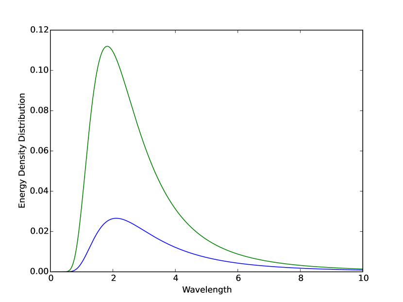
(a) Modified Planck’s Distribution

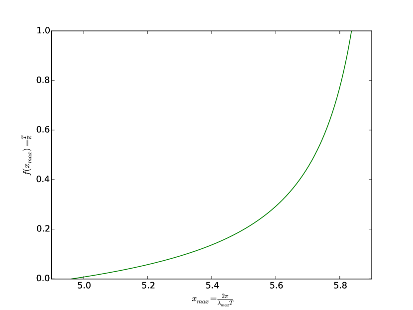
(b) Plot Showing The Modified Nature Of Wien’s Law

Figure 1: The plot (a) shows the Planck energy distribution as a function of wavelength $\lambda$ for both modified and unmodified measures. Here the blue and the green colour correspond to the cases of unmodified and the modified measures respectively. We have taken $a_{0,0}=1.0,$ $a_{0,1}=a_{1,0}=0.2$ and all other $a^{\prime}$s are zero, temperature is $T=0.6$, volume is $10^{35}$ and $\kappa=1$ in Planck units. The plot (b) shows the modification in the Wien’s displacement law. The usual Wien’s law would have given us a constant value of $x_{max}$ corresponding to the point where $f(x_{max})=0$. We can clearly see from the plot that this value is $x_{max}\approx 4.965$. The coefficient $a_{1,0}$ has been taken to be 1. We have chosen the range such that $\frac{T}{\kappa}$ lies between $0$ and $1$. Although to decide the actual range of the possible T-values one needs more thorough and careful thinking, on the other hand in this paper for our purpose we have discussed the only cases where T lies between $0$ and $\kappa=1$.

A typical plot of the modified energy density distribution in comparison to the usual Planck distribution is shown in figure 1(a) on page 1(a). Let us first express the above distribution in terms of wavelength $\lambda$. The energy density between $\omega$ and $\omega+d\omega$ or the corresponding $\lambda$ and $\lambda+d\lambda$ is $u(\lambda)d\lambda=u(\omega)d\omega$ which implies $u(\lambda)=u(\omega)\frac{d\omega}{d\lambda}=-\frac{\omega^{2}u(\omega)}{2\pi}$, where $\omega$ and $\lambda$ are related by $\omega=\frac{2\pi}{\lambda}$. From (3.0.1) we can write $u(\omega)=\sum_{n=0}^{\infty}A_{n}\,\,\frac{\omega^{n+3}}{e^{\frac{\omega}{T}}-1}$ where,

$$A_{n} =\frac{1}{\pi^{2}}\sum_{n^{\prime}=0,n^{\prime}\neq 3}^{\infty}\frac{a_{n,n^{\prime}}}{n!n^{\prime}!\kappa^{n}}\left(\frac{4\pi}{3-n^{\prime}}\right)\frac{1}{\kappa^{3}V_{ac}}\left[\left(\frac{3V\kappa^{3}}{4\pi}\right)^{\frac{3-n^{\prime}}{3}}-1\right]$$

$$+\frac{1}{\pi^{2}}\frac{a_{n,3}}{n!3!\kappa^{n}}\left(\frac{4\pi}{3\kappa^{3}V_{ac}}\right)\ln\left(\frac{3V\kappa^{3}}{4\pi}\right)$$ (3.10)

is a constant and is independent of both $\lambda$ and $T$. We then have,

$$u(\lambda)=-\sum_{n=0}^{\infty}\frac{(2\pi)^{n+4}A_{n}}{\lambda^{n+5}\left(e^{\frac{2\pi}{\lambda T}}-1\right)}.$$ (3.11)

Differentiating with respect to $\lambda$ we get

$$\frac{du(\lambda)}{d\lambda}=\frac{1}{\lambda^{6}\left(e^{\frac{2\pi}{\lambda T}}-1\right)}\sum_{n=0}^{\infty}\frac{(2\pi)^{n+4}A_{n}}{\lambda^{n}}\left[n+5-\frac{\left(\frac{2\pi}{\lambda T}\right)}{1-e^{-\frac{2\pi}{\lambda T}}}\right].$$ (3.12)

Note that in the case of unmodified measure, we have $A_{0}=1/\pi^{2},A_{1}=A_{2}=...=0$ and the above expression reduces to

$$\frac{du(\lambda)}{d\lambda}=\frac{1}{\lambda^{6}\left(e^{\frac{2\pi}{\lambda T}}-1\right)}\frac{(2\pi)^{4}}{\pi^{2}}\left[5-\frac{\left(\frac{2\pi}{\lambda T}\right)}{1-e^{-\frac{2\pi}{\lambda T}}}\right].$$ (3.13)

Thus $u(\lambda)$ is maximum at $\lambda=\lambda_{max}$ which can be found by the extremum condition $\frac{du(\lambda)}{d\lambda}\bigg{|}_{\lambda_{max}}=0$ giving $5=\frac{x_{max}}{1-e^{-x_{max}}}$ where $x_{max}=\frac{2\pi}{\lambda_{max}T}$. The above equation can be numerically solved to get $x_{max}=\frac{2\pi}{\lambda_{max}T}\approx 4.965,\,\,\Rightarrow\lambda_{max}T\approx 1.266$. This behaviour of $\lambda_{max}$ on temperature $T$ is called Wien’s displacement law. Now for the case of modified measure the extremum condition becomes,

$$\sum_{n=0}^{\infty}T^{n}x_{max}^{n}A_{n}\left[n+5-\frac{x_{max}}{1-e^{-x_{max}}}\right]=0.$$ (3.14)

It is obvious that the solution of $x_{max}$ is now dependent on $T$. Thus the value of $x_{max}=\frac{2\pi}{\lambda_{max}T}$ is no more constant, but a function of $T$. To understand the behaviour in a better way, we keep the leading order terms in $\frac{T}{\kappa}$ and $\frac{1}{V^{1/3}\kappa}$ and neglect all the higher order terms i.e. $A_{0}\approx 1/\pi^{2},\quad A_{1}\approx\frac{a_{1,0}}{\pi^{2}\kappa},\quad A_{2}\approx A_{3}\approx...\approx 0$. The extremum condition then becomes

$$\frac{T}{\kappa}=-\frac{1}{x_{max}a_{1,0}}\left(\frac{5-\frac{x_{max}}{1-e^{-x_{max}}}}{6-\frac{x_{max}}{1-e^{-x_{max}}}}\right)=f(x_{max}).$$ (3.15)

We have plotted this function with respect to $x_{max}$ (see figure 1(b) on page 1(b)). For a fixed value of $y-$axis, i.e., a fixed $\frac{T}{\kappa}-$ value the corresponding value of $x_{max}$ can be obtained from the plot. As visible from the plot $x_{max}=\frac{2\pi}{\lambda_{max}T}$ is a monotonically increasing function of $T$, i.e., $f^{-1}(\frac{T}{\kappa})$. This implies $\lambda_{max}=\frac{2\pi}{Tf^{-1}(\frac{T}{\kappa})}$ is a monotonically decreasing function of $T$. Note that $\lambda_{max}$ for modified phase space measure decreases more rapidly with increasing $T$ than the case of unmodified measure where $x_{max}=f^{-1}(\frac{T}{\kappa})$ takes a constant value. The significant change in the values of $x_{max}$ occurs only if the order of the change in temperature is non-negligible with respect to $\kappa$. That is why in SR limit, i.e., $\frac{T}{\kappa}\rightarrow 0$, the $x_{max}=\frac{2\pi}{\lambda_{max}T}$ is almost constant giving the standard Wien’s displacement law. The extremum condition for the unmodified measure corresponds to $f(x_{max})=0$. As it is visible in figure 1(b) on page 1(b) this gives the usual value $x_{max}\approx 4.965$. Note that the value of $f^{-1}\left(\frac{T}{\kappa}\right)$ is always greater than the SR value $4.965$. Hence $\frac{(\lambda_{max})_{DSR}}{(\lambda_{max})_{SR}}=\frac{4.965}{f^{-1}\left(\frac{T}{\kappa}\right)}\leq 1$. Thus, the frequency at which the energy density distribution of blackbody radiation at a given temperature peaks, gets a positive correction. Now, suppose we demand at least $1\%$ correction i.e., $\frac{(\lambda_{max})_{DSR}}{(\lambda_{max})_{SR}}=\frac{4.965}{f^{-1}\left(\frac{T}{\kappa}\right)}=\frac{99}{100}$ then we get $f^{-1}\left(\frac{T}{\kappa}\right)=5.015$. The corresponding $\frac{T}{\kappa}$ from the plot is $0.01$. So, to get an observable effect of DSR using modified Wien’s displacement law one needs to consider a system having temperature in the range of $100$th part of the effective $\kappa$ value. Note that some exotic phenomenon in the semi-classical regime of quantum gravity may reduce the effective value of the energy cut-off in certain specific systems. A similar reduction in the effective value of high energy cut-off has been suggested in a simple quantum mechanical table top experiment in section 6.

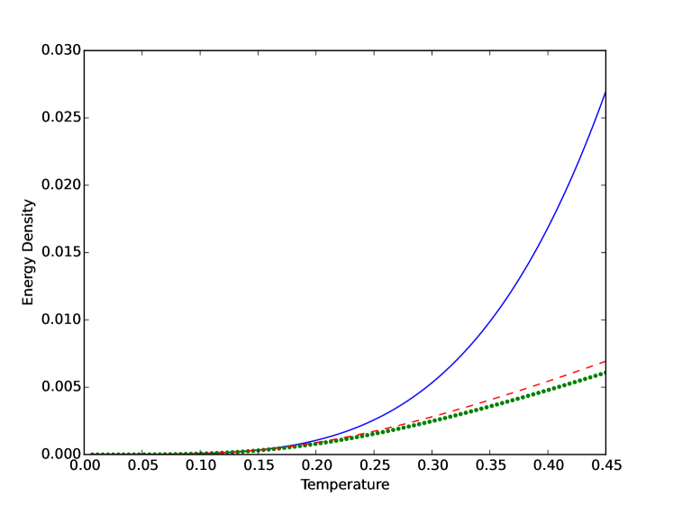
(a) Energy Density Distribution

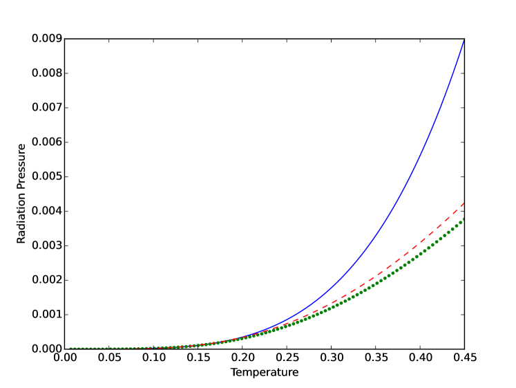
(b) Radiation Pressure

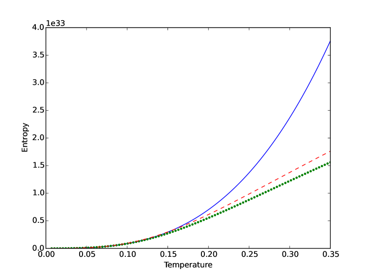
(c) Entropy

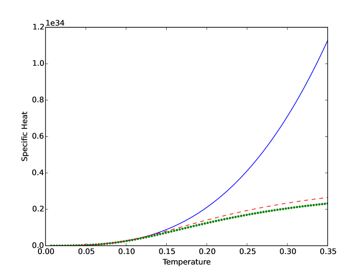
(d) Specific Heat

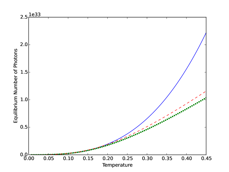
(e) Equilibrium Number Of Photons

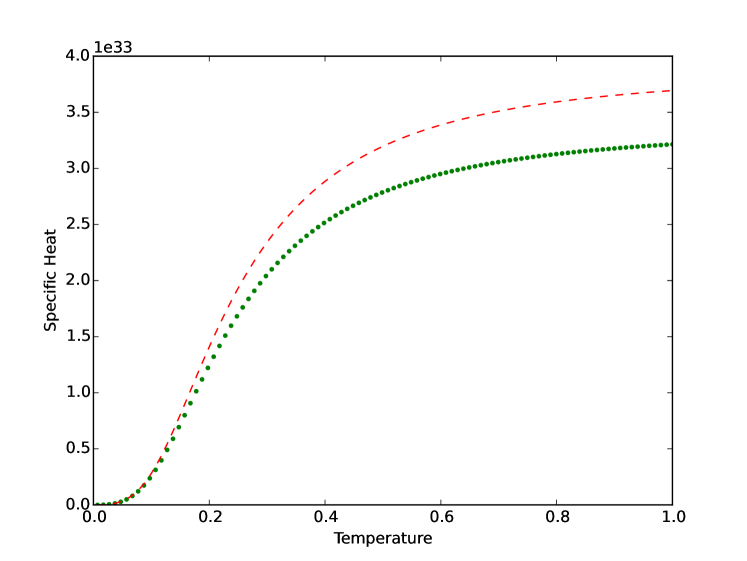
(f) Specific Heat Mimicking Debye Theory

Figure 2: The plots show the variation of energy density, radiation pressure, entropy, specific heat and equilibrium number of photons with temperature for thermodynamic quantities with an ultraviolet energy cut-off and also with the modified measure. The blue solid, the green dotted and the red dashed lines correspond to the SR, the case with the ultraviolet energy cut-off and the case with the modified measure respectively. As is visible from the plots it matches with SR at low T and with increasing T it deviates from SR significantly. Here $\kappa=1$ and $V=10^{35}$ in Planck units and $a_{0,0}=1$, $a_{0,1}=a_{1,0}=0.2$ and all other $a^{\prime}$s are taken to be zero. Note that all the quantities above become approximately linear near $T\rightarrow\kappa$. In the low temperature regime, energy density $u$ and radiation pressure $P$ follow $\sim T^{4}$ behaviour, while the entropy $S$, the specific heat $C_{V}$ and the equilibrium number of photons $\bar{N}$ follow $\sim T^{3}$ behaviour. The behaviour of $C_{V}$ for the full range of $\frac{T}{\kappa}\in[0,1]$ is shown in the figure at bottom right corner, which certainly mimics the Debye theory. In the Debye theory however T may go up to infinity in which case the specific heat goes to a constant value.

3.0.2 Various thermodynamic quantities with modified measure

We have calculated various thermodynamic quantities with the modified measure. The exact results in form of lengthy expressions are listed in B.1 and here we proceed further with physical analysis only. Note that in this case all the thermodynamic quantities reduce to the unmodified case for $n=0$ and $n^{\prime}=0$. Also in the SR limit, we get the usual SR result as expected. The value of the thermodynamic quantities, in this case, can either be less than or equal to (for certain T-values only) or greater than both the SR value and the values in case with only an ultraviolet energy cut-off, depending on the choice of $a_{n,n^{\prime}}$. To plot these quantities we have chosen the $a_{n,n^{\prime}}$ values in such a way that the value of the modified case is more than the unmodified case and less than the SR case. Though it is not visible in the plot because of the chosen $a_{n,n^{\prime}}$ values, but it is a fact that for certain choices of $a_{n,n^{\prime}}$ the modified DSR value becomes equal to the value of SR at some temperatures and can even overshoot the SR curve. The nonanalytic nature in the SR limit for the case of modified measure is similar as in the unmodified case. The leading order behaviour in the low and high temperature limits are discussed in the next section.

4 Effects of DSR in Big Bang and cosmology

In this section we will explore the possible effects of the behaviour of DSR photons near the Planck scale with an invariant ultraviolet energy cut-off. To see the physical applicability of the results with such an invariant ultraviolet energy cut-off one has to, in general, probe near the Planck scale. The results can then be used to study the early Universe thermodynamics especially Big Bang cosmology. Since we have the modified energy density $u$ and Pressure $P$, therefore we have a modified energy-momentum tensor $T_{\mu\nu}$. In general, we should use the modified metric when we are exploring the early Universe near Planck scale. In DSR, Smolin has suggested one such metric called the Rainbow metric [24][58][59] [60][61], but we will not attempt to discuss this here. With the above quantities at hand, we can then solve the Friedmann equations (more specifically FRW equations) and see the possible modification in the known results of the expansion of the Universe after Big Bang at such a scale. This is very involved and a more detailed study can be done separately in future. But we can still consider a scenario where we can see the possible modification near the Big Bang. The FRW and its relation is a standard and well studied cosmology subject. We, for our analysis, will follow chapter 8 of [62]. We will consider the radiation dominated epoch where the modified energy density and pressure is given by (2.5) and (2.3) respectively. With such a modification of $T_{\mu\nu}$, the energy conservation equation (8.54) in section 8.3 of [62] gets modified to

$$\frac{\dot{u}}{u}=-\left(4-\frac{\frac{T{\kappa}^{3}}{{\pi}^{2}}ln(1-e^{-\frac{\kappa}{T}})}{u}\right)\frac{\dot{a}}{a}.$$ (4.1)

We then express $u$ in terms of $T$ to get,

$$H=\frac{\dot{a}}{a}=-\frac{\dot{T}}{T}\left[\frac{24\left[Z_{4}(0)-Z_{4}\left(\frac{\kappa}{T}\right)\right]-\left(\frac{\kappa}{T}\right)^{4}Li_{0}\left(e^{\frac{-\kappa}{T}}\right)}{24\left[Z_{4}(0)-Z_{4}\left(\frac{\kappa}{T}\right)\right]+\left(\frac{\kappa}{T}\right)^{3}Li_{1}\left(e^{\frac{-\kappa}{T}}\right)}\right]$$ (4.2)

Here $a$ is the dimensionless scale factor and $H$ is the Hubble parameter which characterizes the rate of expansion of the Universe. It is easy to see that the numerator is always less than the denominator. Therefore $\frac{H}{H_{SR}}<1$ always, where $H_{SR}=-\frac{\dot{T}}{T}$, which implies that the expansion of the Universe was at a slower rate in the radiation dominated era than the rate of expansion without such modifications. Because of the slower expansion, all the epochs would eventually get delayed resulting in the modification in the age of the known Universe. In the SR limit the modified Hubble parameter becomes nearly equal to the normal SR one, as $\frac{\kappa}{T}$ is very large, so the correction terms go to zero as expected.

We can also see its application in case of “bouncing” loop quantum cosmology theories (see [63][64][65] and the references therein), where normally we consider specific modifications to the spacetime geometry which effectively puts a bound on the curvature and in this way the Big Bang singularity can be avoided. But for such “bouncing” models, we cannot use the perturbation technique at the curvature saturation, as the energy density of the cosmic fluid diverges. What one can do to still avoid the Big Bang singularity is to consider an inflation model where we can safely use the perturbation theory. Here we have obtained the energy density of the cosmic fluid which saturates to the Planck energy which of course is finite. Then we can combine both the results obtained in this paper and the “bouncing” loop quantum cosmology to study the possible way out to avoid the Big Bang singularity.

Next we consider the DSR photons at an effective lower scale due to other parameters in the theory like mass, number density etc. These parameters may effectively lower the Planck scale such that its effects can be observed in very high temperature and high density regimes. To probe such DSR effects we need to observe the stellar objects with very high temperatures and densities. For example, the astronomical data from gamma ray burst during the merging of neutron stars (which has the core temperature of $T=10^{12}$ K) may give a bound on effective $\kappa$ value. We can also explore the Chandrasekhar limits and its possible modifications. The application of the theory developed here has been explored in detail for white dwarfs in [66]. It will also be interesting to see if one gets a better bound on $\kappa$ in case of luminosity calculation of neutron stars using the results obtained for the blackbody radiation in this paper.

5 The leading behaviour for $T\rightarrow 0$ and $T\rightarrow\kappa$

We have plotted various thermodynamic quantities as a function of temperature (see figure 2 on page 2). Let us now analyse the behaviour near $T=0$ and $T=\kappa$. In the low temperature regime we take $\frac{T}{\kappa}=\epsilon<<1$. The low temperature behaviour is as follows,

$$u\approx\frac{{\pi}^{2}\kappa^{4}{\epsilon}^{4}}{15}-\frac{\kappa^{4}}{\pi^{2}}\epsilon e^{-\frac{1}{\epsilon}}\approx\frac{{\pi}^{2}T^{4}}{15},\quad P\approx\frac{{\pi}^{2}T^{4}}{45},$$

$$S\approx\frac{4V_{ac}{\pi}^{2}T^{3}}{45},\quad C_{V}\approx\frac{4V_{ac}{\pi}^{2}T^{3}}{15},\quad\bar{N}\approx\frac{2V_{ac}\zeta(3)T^{3}}{{\pi}^{2}}.$$ (5.1)

Here we have used the fact that $Li_{n}(z)\rightarrow z$ as $z\rightarrow 0$. In the expression for energy density, we have neglected the second term with respect to the first. We can see this by putting $x=\frac{1}{\epsilon}$ and as $x\rightarrow\infty$ the ratio of the second term to the first, in the above equation goes to zero. Note that the second term $\epsilon e^{-\frac{1}{\epsilon}}$ is the nonanalytic piece which makes this limit non-perturbative i.e. this expression cannot be Taylor series expanded in the low temperature limit. Let us consider the energy density relation in the $\frac{T}{\kappa}=\epsilon<<1$ limit, given by $u\approx\frac{{\pi}^{2}\kappa^{4}{\epsilon}^{4}}{15}-\frac{\kappa^{4}}{\pi^{2}}\epsilon e^{-\frac{1}{\epsilon}}$. Now assuming that we get at least $1\%$ correction i.e.,

$$\frac{\frac{\kappa^{4}}{\pi^{2}}\epsilon e^{-\frac{1}{\epsilon}}}{\frac{{\pi}^{2}\kappa^{4}{\epsilon}^{4}}{15}}\geq\frac{1}{100}$$ (5.2)

which, in turn, gives a bound on $\epsilon$ as $0.10\leq\epsilon\leq 2.1$. But since we have taken $\epsilon<<1$, therefore the equality holds at $\epsilon=0.10$. This fact is also visible from the plots of the thermodynamic quantities in which the modified behaviour starts deviating from the SR result at $\frac{T}{\kappa}\sim 10^{-1}$. Another point to note is that the value of $\epsilon$, for at least $1\%$ correction, in case of modified Wien’s displacement law came out to be around $0.01$ (See section 3.0.1). Thus, the modified Wien’s displacement law starts giving an observable correction for the systems having temperature one order less compared to the systems used in case of modified thermodynamic quantities. For pressure we do the similar analysis where the first term in (2.3) is nothing but $\left(\frac{\kappa^{3}T}{3\pi^{2}}\right)Li_{1}(e^{\frac{-\kappa}{T}})$. A similar analysis follows for other thermodynamic quantities as well. Thus in low temperature regime, energy density $u$ and radiation pressure $P$ follow $\sim T^{4}$ behaviour, while the entropy $S$, the specific heat $C_{V}$ and the equilibrium number of photons $\bar{N}$ follow $\sim T^{3}$ behaviour. The nonanalyticity in this limit is a general feature of all the thermodynamic quantities. For high temperature, $T\approx\kappa(1-\epsilon)$ such that $\epsilon<<1$ which gives $\frac{\kappa}{T}\approx 1+\epsilon$. We will expand all the quantities to the leading order in $\epsilon$ and finally put $\epsilon=1-\frac{T}{\kappa}$ to get the leading high temperature behaviour. The results are listed in B.2. Note that to get the linear dependence of $C_{V}$ on $T$ in (B.12) by differentiating the high $T$ behaviour of $U$, we need to expand $U$ up to $T^{2}$ order. All these linear behaviours for $T\rightarrow\kappa$ are very clearly visible in the plots. For the modified measure we get essentially the similar behaviour for both the limits. The results of the leading behaviour in case of modified measure are listed in B.3 and B.4.

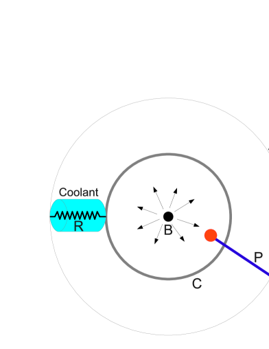
Figure 3: A quantum mechanical table top experiment for testing the theory. Here B is a perfect blackbody surrounded by a spherical cathode C, which is enclosed by a spherical anode A and the circuit is completed using a high resistance resistor R. All the radiations above the frequency $\nu_{th}$ corresponding to the photoelectric threshold of the cathode are absorbed and will be lost as Joule heating through R. The resistor is continuously being cooled by coolant, shown in blue colour, to avoid the melting of the resistor. The photons below the frequency $\nu_{th}$ stay inside the cavity surrounded by the cathode C and behave as acoustic phonons as shown in this paper. The properties of these photons acting as acoustic phonons can be measured by inserting a probe P connected with the measuring instrument.

6 Effective low energy realizations of the theory

In this section, we present the possibilities of physical realization of the results obtained with an effective cut-off for the photons such that they behave as phonons. As is clear from the description this cut-off might not be invariant which was the case in the other applications discussed above. But this is an interesting case in its own regard, as we have a way to get a bunch of photons behaving as phonons and they can be observed in a laboratory as well. To start with here we will be suggesting a simple table top experiment to test the result obtained in section 2. Note that due to no change in dispersion relation the only effect on the thermodynamics of a photon gas is due to the high energy cut-off. If one can introduce such a cut-off on the photon energy in some experiment then the photons will start behaving like acoustic phonons. Consider a perfect blackbody (see figure 3 on page 3) surrounded by a spherical cathode which is enclosed by a spherical anode and the circuit being completed using a high resistance. Now, suppose the cathode has the photoelectric threshold $\nu_{th}$ such that all the radiations above frequency $\nu_{th}$ gets absorbed by the cathode. These absorbed radiations lead to the Joule heating of the resistor which is then cooled by an appropriate coolant. Since, we do not want the heating of the resistor, in any way, to affect the radiations inside the cathode, therefore the cathode may be coated with an insulating material. Another possible alternative is to drill a small hole in anode then connect the resistor outside and far away from the anode where it can be cooled. Now, we are left with photons in the cathode cavity, with energy less than $\kappa=\nu_{th}$ which is the desired cut-off in the theory. We, therefore, have generated photons inside the cathode which mimic acoustic phonons. To observe this we can now drill a very small hole in both anode and cathode, through which a probe, connected to the measuring instrument, can be inserted to test the properties of the photons. To observe at least $1\%$ deviation (see the discussion in section 5) from the usual photon thermodynamics at room temperature $T=293$ K the material of the cathode can be selected with threshold $\nu_{th}=\frac{k_{B}T}{0.1h}=6.1\times 10^{13}Hz$ (here we have put the actual values of $h$ and $k_{B}$). Many commercially available materials fall into this category.

7 Summary and future works

We started with the DSR formalism by MS where the modified dispersion relation, in order to incorporate an invariant energy scale $\kappa$, is given by (1.1). But in the case of photon gas, it is simply $\varepsilon=p$. Since there is a cut-off on the maximum energy and the minimum length, the expression of the thermodynamic quantities changes accordingly. We started by considering a model of a photon gas obeying Bose-Einstein statistics in grand canonical ensemble and went on calculating various thermodynamic quantities such as energy density, pressure, entropy, specific heat and equilibrium number of photons with such an ultraviolet cut-off. We found one to one correspondence between the behaviour of photons with an ultraviolet cut-off and the acoustic phonons in the Debye theory. The Stefan-Boltzmann law got modified which will give correction to the dynamics of many stellar objects. We found that the non-perturbative nature of the thermodynamic quantities in the SR limit is a general feature of the theory with an ultraviolet energy cut-off. We also noted that the values of all the thermodynamic quantities are less than the SR values because of this cut-off. We then studied the change in the phase space measure for exotic spacetimes at Planck scale and discussed the example of classical ideal gas for illustration. We found that the classical ideal gas in case of modified phase space measure has a non-trivial volume dependence in its expression for the partition function leading to the modification in the thermodynamic quantities like pressure accordingly. We went on calculating the possible change in the thermodynamic quantities due to the change in the phase space measure. Because of this modification, Planck’s energy density distribution and the Wien’s displacement law got modified. Note that all the thermodynamic quantities reduce to the usual SR result in $\kappa\rightarrow\infty$ limit. We have plotted the temperature dependence of various thermodynamic quantities. We can clearly see from the plots of various thermodynamic quantities that we start getting the deviation of the results obtained in the modified case from the SR case at $\frac{T}{\kappa}\sim 10^{-1}$. We found that the modified Wien’s law can be observed at comparatively lower temperature than the thermodynamic quantities. Next, we discussed the possible realization of the modification at Planck scale by considering its effects near the Big Bang. The effectively lower Planck scale cosmological observations and modifications of DSR have also been discussed. The leading behaviour for $T\rightarrow 0$ and $T\rightarrow\kappa$ have been analysed. We observed that in the case of modified phase space measure the values of the thermodynamic quantities might be less than, equal to or greater than the SR values depending on the choice of $a_{n,n^{\prime}}$. As was seen both for the case with only an ultraviolet cut-off and the modified measures, the nonanalyticity in the special relativistic limit is a general feature of the energy cut-off introduced in the theory. In the last section, we have given the possible scenarios of the physical observation of results obtained in effective low energy by suggesting a quantum mechanical table top experiment. Note that the present work only deals with the study of massless bosons i.e. photons, but the analysis can be extended to massive bosons and fermions as well. This will give us an insight into the invariant energy scale effects in well-known phenomenon such as Bose-Einstein condensation and the behaviour of degenerate Fermi gas. This, in turn, leads to the study of the stellar objects such as white dwarfs and neutron stars. It would certainly be interesting to see whether the non-perturbative effects appear in such massive cases too. Analysis of this paper can be used to study early Universe thermodynamics.

Appendix A Criterion for swapping the double summation and the integral

The interchange of summation and integration signs for a series is a well known theorem (see theorem 1.38 of [67]). In this Appendix, we will generalize this theorem for a double series i.e. we will prove the equality,

$$\int_{\mathcal{M}}\sum_{n}\sum_{n^{\prime}}A_{n,n^{\prime}}=\sum_{n}\sum_{n^{\prime}}\int_{\mathcal{M}}A_{n,n^{\prime}}$$ (A.1)

holds if,

$$\sum_{n}\sum_{n^{\prime}}\int_{\mathcal{M}}|A_{n,n^{\prime}}|<\infty.$$ (A.2)

We take the two summations out of the integral one by one in the LHS of (A.1) to get the RHS, using theorem 1.38 of [67] which is allowed if,

$$\sum_{n}\int_{\mathcal{M}}\left|\sum_{n^{\prime}}A_{n,n^{\prime}}\right|<\infty\quad\rm{and}\quad\sum_{n^{\prime}}\int_{\mathcal{M}}|A_{n,n^{\prime}}|<\infty\quad\forall n.$$ (A.3)

Let us rewrite (A.2) as,

$$\sum_{n}t_{n}<\infty\quad\rm{with}\quad t_{n}=\sum_{n^{\prime}}\int_{\mathcal{M}}|A_{n,n^{\prime}}|\quad\forall n.$$ (A.4)

We note that $t_{n}\geq 0\quad\forall n$, which along with (A.4) implies $t_{n}<\infty\quad\forall n$ which is nothing but the second inequality in (A.3). This further implies (because of theorem 1.38 of [67]),

$$t_{n}=\int_{\mathcal{M}}\sum_{n^{\prime}}|A_{n,n^{\prime}}|\quad\forall n.$$ (A.5)

Now we note that $\left|\sum_{n^{\prime}}A_{n,n^{\prime}}\right|\leq\sum_{n^{\prime}}|A_{n,n^{\prime}}|\quad\forall n$. Integrating over $\mathcal{M}$ followed by the summation over $n$ we get,

$$\sum_{n}\int_{\mathcal{M}}\left|\sum_{n^{\prime}}A_{n,n^{\prime}}\right| \leq\sum_{n}\int_{\mathcal{M}}\sum_{n^{\prime}}|A_{n,n^{\prime}}|\quad\forall n$$ (A.6)

Taking (A.5) and (A.4) into account in the above inequality we get the first inequality of (A.3). Thus we have proved that (A.2) implies (A.3) and hence if (A.2) is satisfied then the equality (A.1) holds true.

Appendix B List of certain results

B.1 Thermodynamic quantities with modified measure

Following what we did in section 2.1 along with using (3.0.1) we get,

$$u =\frac{1}{\left(\pi\right)^{2}}\displaystyle{\sum_{n=0,n^{\prime}=0\atop n^{\prime}\neq 3}^{\infty}}\frac{a_{n,n^{\prime}}}{n!n^{\prime}!\kappa^{n}}\frac{4\pi}{\left(3-n^{\prime}\right)}\bigg{(}\frac{T^{n+4}}{V_{ac}\kappa^{3}}\bigg{)}\left[\left(\frac{3V\kappa^{3}}{4\pi}\right)^{\frac{3-n^{\prime}}{3}}-1\right]\Gamma(n+4)\bigg{[}Z_{n+4}(0)-Z_{n+4}\left(\frac{\kappa}{T}\right)\bigg{]}$$

$$+\frac{1}{\left(\pi\right)^{2}}\displaystyle{\sum_{n=0}^{\infty}}\frac{a_{n,3}}{n!3!\kappa^{n}}\bigg{(}\frac{4\pi T^{n+4}}{3V_{ac}\kappa^{3}}\bigg{)}\ln\bigg{(}\frac{3\kappa^{3}V}{4\pi}\bigg{)}\Gamma(n+4)\bigg{[}Z_{n+4}(0)-Z_{n+4}\left(\frac{\kappa}{T}\right)\bigg{]}$$

$$=\displaystyle{\sum_{n=0,n^{\prime}=0}^{\infty}}u_{n,n^{\prime}}.$$ (B.1)

Here $u_{n,n^{\prime}}$ is a general term of the summation. Therefore the specific heat capacity $C_{V}$ is,

$$C_{V} =\bigg{(}\frac{\partial U}{\partial T}\bigg{)}_{V_{ac}}=\displaystyle{\sum_{n=0,n^{\prime}=0\atop n^{\prime}\neq 3}^{\infty}}\left[\frac{1}{\left(\pi\right)^{2}}\frac{a_{n,n^{\prime}}}{n!n^{\prime}!\kappa^{n+3}}\frac{4\pi}{\left(3-n^{\prime}\right)}\left[\left(\frac{3V\kappa^{3}}{4\pi}\right)^{\frac{3-n^{\prime}}{3}}-1\right]\bigg{\{}\frac{1}{(1-e^{\frac{\kappa}{T}})}\frac{\kappa^{n+4}}{T}\bigg{\}}+(n+4)\left(\frac{u_{n,n^{\prime}}V_{ac}}{T}\right)\right]$$

$$+\displaystyle{\sum_{n=0}^{\infty}}\left[\frac{1}{\left(\pi\right)^{2}}\frac{a_{n,3}}{n!3!\kappa^{n+3}}\left(\frac{4\pi}{3}\right)\ln\bigg{(}\frac{3\kappa^{3}V}{4\pi}\bigg{)}\bigg{\{}\frac{1}{(1-e^{\frac{\kappa}{T}})}\frac{\kappa^{n+4}}{T}\bigg{\}}+(n+4)\left(\frac{u_{n,3}V_{ac}}{T}\right)\right].$$ (B.2)

The radiation pressure can easily be calculated in essentially the similar manner to get,

$$P =\frac{1}{\left(\pi\right)^{2}}\displaystyle{\sum_{n=0,n^{\prime}=0\atop n^{\prime}\neq 3}^{\infty}}\frac{a_{n,n^{\prime}}}{n!n^{\prime}!\kappa^{n}}\frac{4\pi}{\left(3-n^{\prime}\right)}\bigg{(}\frac{T}{V_{ac}\kappa^{3}}\bigg{)}\left[\left(\frac{3V\kappa^{3}}{4\pi}\right)^{\frac{3-n^{\prime}}{3}}-1\right]\bigg{\{}-\ln(1-e^{-\frac{\kappa}{T}})\frac{\kappa^{n+3}}{n+3}+\frac{T^{n+3}}{(n+3)}\Gamma(n+4)\bigg{[}Z_{n+4}(0)$$

$$-Z_{n+4}\left(\frac{\kappa}{T}\right)\bigg{]}\bigg{\}}+\frac{1}{\left(\pi\right)^{2}}\displaystyle{\sum_{n=0}^{\infty}}\frac{a_{n,3}}{n!3!\kappa^{n}}\bigg{(}\frac{4\pi T}{3V_{ac}\kappa^{3}}\bigg{)}\ln\bigg{(}\frac{3\kappa^{3}V}{4\pi}\bigg{)}\bigg{\{}-\ln(1-e^{-\frac{\kappa}{T}})\frac{\kappa^{n+3}}{n+3}+\frac{T^{n+3}}{(n+3)}\Gamma(n+4)\bigg{[}Z_{n+4}(0)-Z_{n+4}\left(\frac{\kappa}{T}\right)\bigg{]}\bigg{\}}.$$ (B.3)

This can be related to the energy density as

$$P =\displaystyle{\sum_{n=0,n^{\prime}=0\atop n^{\prime}\neq 3}^{\infty}}\left[\frac{1}{\left(\pi\right)^{2}}\frac{a_{n,n^{\prime}}}{n!n^{\prime}!\kappa^{n}}\frac{4\pi}{\left(3-n^{\prime}\right)}\bigg{(}\frac{T}{V_{ac}\kappa^{3}}\bigg{)}\left[\left(\frac{3V\kappa^{3}}{4\pi}\right)^{\frac{3-n^{\prime}}{3}}-1\right]\bigg{\{}-\ln(1-e^{-\frac{\kappa}{T}})\frac{\kappa^{n+3}}{n+3}\bigg{\}}+\frac{u_{n,n^{\prime}}}{(n+3)}\right]$$

$$+\displaystyle{\sum_{n=0}^{\infty}}\left[\frac{1}{\left(\pi\right)^{2}}\frac{a_{n,3}}{n!3!\kappa^{n}}\bigg{(}\frac{4\pi T}{3V_{ac}\kappa^{3}}\bigg{)}\ln\bigg{(}\frac{3\kappa^{3}V}{4\pi}\bigg{)}\bigg{\{}-\ln(1-e^{-\frac{\kappa}{T}})\frac{\kappa^{n+3}}{n+3}\bigg{\}}+\frac{u_{n,3}}{(n+3)}\right].$$ (B.4)

The Helmholtz free energy is,

$$A =\mu N-PV_{ac}=-PV_{ac}$$

$$=\displaystyle{\sum_{n=0,n^{\prime}=0\atop n^{\prime}\neq 3}^{\infty}}\left[\frac{1}{\left(\pi\right)^{2}}\frac{a_{n,n^{\prime}}}{n!n^{\prime}!\kappa^{n+3}}\frac{4\pi T}{\left(3-n^{\prime}\right)}\left[\left(\frac{3V\kappa^{3}}{4\pi}\right)^{\frac{3-n^{\prime}}{3}}-1\right]\bigg{\{}\ln(1-e^{-\frac{\kappa}{T}})\frac{\kappa^{n+3}}{n+3}\bigg{\}}-\frac{u_{n,n^{\prime}}V_{ac}}{(n+3)}\right]$$

$$+\displaystyle{\sum_{n=0}^{\infty}}\frac{a_{n,3}}{n!3!\kappa^{n+3}}\left[\frac{1}{\left(\pi\right)^{2}}\left(\frac{4\pi T}{3}\right)\ln\bigg{(}\frac{3\kappa^{3}V}{4\pi}\bigg{)}\bigg{\{}\ln(1-e^{-\frac{\kappa}{T}})\frac{\kappa^{n+3}}{n+3}\bigg{\}}-\frac{u_{n,3}V_{ac}}{(n+3)}\right].$$ (B.5)

And the entropy becomes,

$$S=\frac{U-A}{T} =\displaystyle{\sum_{n=0,n^{\prime}=0\atop n^{\prime}\neq 3}^{\infty}}\left[\frac{1}{\left(\pi\right)^{2}}\frac{a_{n,n^{\prime}}}{n!n^{\prime}!\kappa^{n+3}}\frac{4\pi}{\left(3-n^{\prime}\right)}\left[\left(\frac{3V\kappa^{3}}{4\pi}\right)^{\frac{3-n^{\prime}}{3}}-1\right]\bigg{\{}-\ln(1-e^{-\frac{\kappa}{T}})\frac{\kappa^{n+3}}{n+3}\bigg{\}}+\frac{(n+4)}{(n+3)}\left(\frac{u_{n,n^{\prime}}V_{ac}}{T}\right)\right]$$

$$+\displaystyle{\sum_{n=0}^{\infty}}\left[\frac{1}{\left(\pi\right)^{2}}\frac{a_{n,3}}{n!3!\kappa^{n+3}}\left(\frac{4\pi}{3}\right)\ln\bigg{(}\frac{3\kappa^{3}V}{4\pi}\bigg{)}\bigg{\{}-\ln(1-e^{-\frac{\kappa}{T}})\frac{\kappa^{n+3}}{n+3}\bigg{\}}+\frac{(n+4)}{(n+3)}\left(\frac{u_{n,3}V_{ac}}{T}\right)\right].$$ (B.6)

The equilibrium number of photons in modified measure can be estimated in the same way as we did in unmodified case and using (3.0.1) we have,

$$\bar{N} =\frac{1}{\left(\pi\right)^{2}}\displaystyle{\sum_{n=0,n^{\prime}=0\atop n^{\prime}\neq 3}^{\infty}}\frac{a_{n,n^{\prime}}}{n!n^{\prime}!k^{n+3}}\frac{4\pi T^{n+3}}{\left(3-n^{\prime}\right)}\left[\left(\frac{3V\kappa^{3}}{4\pi}\right)^{\frac{3-n^{\prime}}{3}}-1\right]\Gamma(n+3)\bigg{[}Z_{n+3}(0)-Z_{n+3}\left(\frac{\kappa}{T}\right)\bigg{]}$$

$$+\frac{1}{\left(\pi\right)^{2}}\displaystyle{\sum_{n=0}^{\infty}}\frac{a_{n,3}}{n!3!\kappa^{n+3}}\left(\frac{4\pi T^{n+3}}{3}\right)\ln\bigg{(}\frac{3\kappa^{3}V}{4\pi}\bigg{)}\Gamma(n+3)\bigg{[}Z_{n+3}(0)-Z_{n+3}\left(\frac{\kappa}{T}\right)\bigg{]}.$$ (B.7)

B.2 The leading high temperature behaviour for unmodified case

In the high temperature ($T\rightarrow\kappa$) case we get,

$$u\approx-\frac{18\kappa^{4}}{\pi^{2}}\left[Z_{4}(0)-Z_{4}(1)-\frac{1}{18(e-1)}\right]+\frac{24\kappa^{4}}{\pi^{2}}\left(\frac{T}{\kappa}\right)\left[Z_{4}(0)-Z_{4}(1)-\frac{1}{24(e-1)}\right],$$ (B.8)

$$P\approx-\frac{6\kappa^{4}}{\pi^{2}}\left[Z_{4}(0)-Z_{4}(1)\right]+\frac{8\kappa^{4}}{\pi^{2}}\left(\frac{T}{\kappa}\right)\left[Z_{4}(0)-Z_{4}(1)\right]-\frac{\kappa^{4}}{3\pi^{2}}\left(\frac{T}{\kappa}\right)\ln\left(1-\frac{1}{e}\right),$$ (B.9)

$$S\approx-\frac{\kappa^{3}V_{ac}}{3\pi^{2}}\ln\left(1-\frac{1}{e}\right)-\frac{16\kappa^{3}V_{ac}}{\pi^{2}}\left[Z_{4}(0)-Z_{4}(1)-\frac{1}{48(e-1)}\right]+\frac{24\kappa^{3}V_{ac}}{\pi^{2}}\left(\frac{T}{\kappa}\right)\left[Z_{4}(0)-Z_{4}(1)-\frac{1}{24(e-1)}\right],$$ (B.10)

$$\bar{N}\approx-\frac{4\kappa^{3}V_{ac}}{\pi^{2}}\left[Z_{3}(0)-Z_{3}(1)-\frac{1}{4(e-1)}\right]+\frac{6\kappa^{3}V_{ac}}{\pi^{2}}\left(\frac{T}{\kappa}\right)\left[Z_{3}(0)-Z_{3}(1)-\frac{1}{6(e-1)}\right]$$ (B.11)

and

$$C_{V}\approx-\frac{48\kappa^{3}V_{ac}}{\pi^{2}}\left[Z_{4}(0)-Z_{4}(1)-\frac{(3e-2)}{48(e-1)^{2}}\right]+\frac{72\kappa^{3}V_{ac}}{\pi^{2}}\left(\frac{T}{\kappa}\right)\left[Z_{4}(0)-Z_{4}(1)-\frac{(4e-3)}{72(e-1)^{2}}\right].$$ (B.12)

B.3 The leading low temperature behaviour for modified case

The low temperature limit can be calculated as we did in case of unmodified measure to get,

$$u \approx\frac{1}{\left(\pi\right)^{2}}\displaystyle{\sum_{n=0,n^{\prime}=0\atop n^{\prime}\neq 3}^{\infty}}\frac{a_{n,n^{\prime}}}{n!n^{\prime}!\kappa^{n}}\frac{4\pi}{\left(3-n^{\prime}\right)}\bigg{(}\frac{T^{n+4}}{V_{ac}\kappa^{3}}\bigg{)}\left[\left(\frac{3V\kappa^{3}}{4\pi}\right)^{\frac{3-n^{\prime}}{3}}-1\right]\Gamma(n+4)Z_{n+4}(0)$$

$$+\frac{1}{\left(\pi\right)^{2}}\displaystyle{\sum_{n=0}^{\infty}}\frac{a_{n,3}}{n!3!\kappa^{n}}\bigg{(}\frac{4\pi T^{n+4}}{3V_{ac}\kappa^{3}}\bigg{)}\ln\bigg{(}\frac{3\kappa^{3}V}{4\pi}\bigg{)}\Gamma(n+4)Z_{n+4}(0),$$ (B.13)

$$P \approx\frac{1}{\left(\pi\right)^{2}}\displaystyle{\sum_{n=0,n^{\prime}=0\atop n^{\prime}\neq 3}^{\infty}}\frac{a_{n,n^{\prime}}}{n!n^{\prime}!\kappa^{n}}\frac{4\pi}{\left(3-n^{\prime}\right)}\bigg{(}\frac{T^{n+4}}{V_{ac}\kappa^{3}}\bigg{)}\left[\left(\frac{3V\kappa^{3}}{4\pi}\right)^{\frac{3-n^{\prime}}{3}}-1\right]\frac{\Gamma(n+4)}{(n+3)}Z_{n+4}(0)$$

$$+\frac{1}{\left(\pi\right)^{2}}\displaystyle{\sum_{n=0}^{\infty}}\frac{a_{n,3}}{n!3!\kappa^{n}}\bigg{(}\frac{4\pi T^{n+4}}{3V_{ac}\kappa^{3}}\bigg{)}\ln\bigg{(}\frac{3\kappa^{3}V}{4\pi}\bigg{)}\frac{\Gamma(n+4)}{(n+3)}Z_{n+4}(0),$$ (B.14)

$$S \approx\frac{1}{\left(\pi\right)^{2}}\displaystyle{\sum_{n=0,n^{\prime}=0\atop n^{\prime}\neq 3}^{\infty}}\frac{a_{n,n^{\prime}}}{n!n^{\prime}!\kappa^{n}}\frac{4\pi}{\left(3-n^{\prime}\right)}\bigg{(}\frac{T^{n+3}}{\kappa^{3}}\bigg{)}\left[\left(\frac{3V\kappa^{3}}{4\pi}\right)^{\frac{3-n^{\prime}}{3}}-1\right]\frac{\Gamma(n+4)(n+4)}{(n+3)}Z_{n+4}(0)$$

$$+\frac{1}{\left(\pi\right)^{2}}\displaystyle{\sum_{n=0}^{\infty}}\frac{a_{n,3}}{n!3!\kappa^{n}}\bigg{(}\frac{4\pi T^{n+3}}{3\kappa^{3}}\bigg{)}\ln\bigg{(}\frac{3\kappa^{3}V}{4\pi}\bigg{)}\frac{\Gamma(n+4)(n+4)}{(n+3)}Z_{n+4}(0),$$ (B.15)

$$C_{V} \approx\frac{1}{\left(\pi\right)^{2}}\displaystyle{\sum_{n=0,n^{\prime}=0\atop n^{\prime}\neq 3}^{\infty}}\frac{a_{n,n^{\prime}}}{n!n^{\prime}!\kappa^{n}}\frac{4\pi}{\left(3-n^{\prime}\right)}\bigg{(}\frac{T^{n+3}}{\kappa^{3}}\bigg{)}\left[\left(\frac{3V\kappa^{3}}{4\pi}\right)^{\frac{3-n^{\prime}}{3}}-1\right]\Gamma(n+4)(n+4)Z_{n+4}(0)$$

$$+\frac{1}{\left(\pi\right)^{2}}\displaystyle{\sum_{n=0}^{\infty}}\frac{a_{n,3}}{n!3!\kappa^{n}}\bigg{(}\frac{4\pi T^{n+3}}{3\kappa^{3}}\bigg{)}\ln\bigg{(}\frac{3\kappa^{3}V}{4\pi}\bigg{)}\Gamma(n+4)(n+4)Z_{n+4}(0)$$ (B.16)

and

$$\bar{N} \approx\frac{1}{\left(\pi\right)^{2}}\displaystyle{\sum_{n=0,n^{\prime}=0\atop n^{\prime}\neq 3}^{\infty}}\frac{a_{n,n^{\prime}}}{n!n^{\prime}!k^{n+3}}\frac{4\pi T^{n+3}}{\left(3-n^{\prime}\right)}\left[\left(\frac{3V\kappa^{3}}{4\pi}\right)^{\frac{3-n^{\prime}}{3}}-1\right]\Gamma(n+3)Z_{n+3}(0)$$

$$+\frac{1}{\left(\pi\right)^{2}}\displaystyle{\sum_{n=0}^{\infty}}\frac{a_{n,3}}{n!3!\kappa^{n+3}}\left(\frac{4\pi T^{n+3}}{3}\right)\ln\bigg{(}\frac{3\kappa^{3}V}{4\pi}\bigg{)}\Gamma(n+3)Z_{n+3}(0)$$ (B.17)

B.4 The leading high temperature behaviour for modified case

In high temperature ($T\rightarrow\kappa$) case the behaviour is

$$u\approx u_{a}+u_{b}T$$ (B.18)

where $u_{a}$ and $u_{b}$ is

$$u_{a} =-\frac{1}{\left(\pi\right)^{2}}\displaystyle{\sum_{n=0,n^{\prime}=0\atop n^{\prime}\neq 3}^{\infty}}\frac{a_{n,n^{\prime}}}{n!n^{\prime}!}\frac{4\pi}{\left(3-n^{\prime}\right)}\bigg{(}\frac{\kappa^{4}}{V_{ac}\kappa^{3}}\bigg{)}\left[\left(\frac{3V\kappa^{3}}{4\pi}\right)^{\frac{3-n^{\prime}}{3}}-1\right]\Gamma(n+4)(n+3)\bigg{[}Z_{n+4}(0)-Z_{n+4}(1)-\frac{1}{(n+3)!(n+3)(e-1)}\bigg{]}$$

$$-\frac{1}{\left(\pi\right)^{2}}\displaystyle{\sum_{n=0}^{\infty}}\frac{a_{n,3}}{n!3!}\bigg{(}\frac{4\pi\kappa^{4}}{3V_{ac}\kappa^{3}}\bigg{)}\ln\bigg{(}\frac{3\kappa^{3}V}{4\pi}\bigg{)}\Gamma(n+4)(n+3)\bigg{[}Z_{n+4}(0)-Z_{n+4}(1)-\frac{1}{(n+3)!(n+3)(e-1)}\bigg{]}$$ (B.19)

$$u_{b} =\frac{1}{\left(\pi\right)^{2}}\displaystyle{\sum_{n=0,n^{\prime}=0\atop n^{\prime}\neq 3}^{\infty}}\frac{a_{n,n^{\prime}}}{n!n^{\prime}!}\frac{4\pi}{\left(3-n^{\prime}\right)}\bigg{(}\frac{\kappa^{4}}{V_{ac}\kappa^{3}}\bigg{)}\left[\left(\frac{3V\kappa^{3}}{4\pi}\right)^{\frac{3-n^{\prime}}{3}}-1\right]\Gamma(n+4)\frac{(n+4)}{\kappa}\bigg{[}Z_{n+4}(0)-Z_{n+4}(1)-\frac{1}{(n+3)!(n+4)(e-1)}\bigg{]}$$

$$+\frac{1}{\left(\pi\right)^{2}}\displaystyle{\sum_{n=0}^{\infty}}\frac{a_{n,3}}{n!3!}\bigg{(}\frac{4\pi\kappa^{4}}{3V_{ac}\kappa^{3}}\bigg{)}\ln\bigg{(}\frac{3\kappa^{3}V}{4\pi}\bigg{)}\Gamma(n+4)\frac{(n+4)}{\kappa}\bigg{[}Z_{n+4}(0)-Z_{n+4}(1)-\frac{1}{(n+3)!(n+4)(e-1)}\bigg{]},$$ (B.20)

$$P\approx P_{a}+P_{b}T$$ (B.21)

where $P_{a}$ and $P_{b}$ is

$$P_{a} =-\frac{1}{\left(\pi\right)^{2}}\displaystyle{\sum_{n=0,n^{\prime}=0\atop n^{\prime}\neq 3}^{\infty}}\frac{a_{n,n^{\prime}}}{n!n^{\prime}!}\frac{4\pi}{\left(3-n^{\prime}\right)}\bigg{(}\frac{\kappa^{4}}{V_{ac}\kappa^{3}}\bigg{)}\left[\left(\frac{3V\kappa^{3}}{4\pi}\right)^{\frac{3-n^{\prime}}{3}}-1\right]\Gamma(n+4)\bigg{[}Z_{n+4}(0)-Z_{n+4}(1)\bigg{]}$$

$$-\frac{1}{\left(\pi\right)^{2}}\displaystyle{\sum_{n=0}^{\infty}}\frac{a_{n,3}}{n!3!}\bigg{(}\frac{4\pi\kappa^{4}}{3V_{ac}\kappa^{3}}\bigg{)}\ln\bigg{(}\frac{3\kappa^{3}V}{4\pi}\bigg{)}\Gamma(n+4)\bigg{[}Z_{n+4}(0)-Z_{n+4}(1)\bigg{]}$$ (B.22)

$$P_{b} =\frac{1}{\left(\pi\right)^{2}}\displaystyle{\sum_{n=0,n^{\prime}=0\atop n^{\prime}\neq 3}^{\infty}}\frac{a_{n,n^{\prime}}}{n!n^{\prime}!}\frac{4\pi}{\left(3-n^{\prime}\right)}\bigg{(}\frac{\kappa^{4}}{V_{ac}\kappa^{3}}\bigg{)}\left[\left(\frac{3V\kappa^{3}}{4\pi}\right)^{\frac{3-n^{\prime}}{3}}-1\right]\left\{\Gamma(n+4)\frac{(n+4)}{\kappa(n+3)}\bigg{[}Z_{n+4}(0)-Z_{n+4}(1)\bigg{]}-\frac{1}{\kappa(n+3)}\ln\left(1-\frac{1}{e}\right)\right\}$$

$$+\frac{1}{\left(\pi\right)^{2}}\displaystyle{\sum_{n=0}^{\infty}}\frac{a_{n,3}}{n!3!}\bigg{(}\frac{4\pi\kappa^{4}}{3V_{ac}\kappa^{3}}\bigg{)}\ln\bigg{(}\frac{3\kappa^{3}V}{4\pi}\bigg{)}\left\{\Gamma(n+4)\frac{(n+4)}{\kappa(n+3)}\bigg{[}Z_{n+4}(0)-Z_{n+4}(1)\bigg{]}-\frac{1}{\kappa(n+3)}\ln\left(1-\frac{1}{e}\right)\right\},$$ (B.23)

$$S\approx S_{a}+S_{b}T$$ (B.24)

where $S_{a}$ and $S_{b}$ is

$$S_{a} =-\frac{1}{\left(\pi\right)^{2}}\displaystyle{\sum_{n=0,n^{\prime}=0\atop n^{\prime}\neq 3}^{\infty}}\frac{a_{n,n^{\prime}}}{n!n^{\prime}!}\frac{4\pi}{\left(3-n^{\prime}\right)}\left[\left(\frac{3V\kappa^{3}}{4\pi}\right)^{\frac{3-n^{\prime}}{3}}-1\right]\frac{1}{(n+3)}\bigg{\{}\Gamma(n+4)(n+4)(n+2)\bigg{[}Z_{n+4}(0)-Z_{n+4}(1)$$

$$-\frac{1}{(n+3)!(n+2)(e-1)}\bigg{]}+\frac{1}{(e-1)}+\ln\left(1-\frac{1}{e}\right)\bigg{\}}$$

$$-\frac{1}{\left(\pi\right)^{2}}\displaystyle{\sum_{n=0}^{\infty}}\frac{a_{n,3}}{n!3!}\bigg{(}\frac{4\pi}{3}\bigg{)}\ln\bigg{(}\frac{3\kappa^{3}V}{4\pi}\bigg{)}\frac{1}{(n+3)}\bigg{\{}\Gamma(n+4)(n+4)(n+2)\bigg{[}Z_{n+4}(0)-Z_{n+4}(1)$$

$$-\frac{1}{(n+3)!(n+2)(e-1)}\bigg{]}+\frac{1}{(e-1)}+\ln\left(1-\frac{1}{e}\right)\bigg{\}}$$ (B.25)

$$S_{b} =-\frac{1}{\left(\pi\right)^{2}}\displaystyle{\sum_{n=0,n^{\prime}=0\atop n^{\prime}\neq 3}^{\infty}}\frac{a_{n,n^{\prime}}}{n!n^{\prime}!}\frac{4\pi}{\left(3-n^{\prime}\right)}\left[\left(\frac{3V\kappa^{3}}{4\pi}\right)^{\frac{3-n^{\prime}}{3}}-1\right]\bigg{\{}\Gamma(n+4)\frac{(n+4)}{\kappa}\bigg{[}Z_{n+4}(0)-Z_{n+4}(1)$$

$$-\frac{1}{(n+3)!(n+4)(e-1)}\bigg{]}\bigg{\}}$$

$$-\frac{1}{\left(\pi\right)^{2}}\displaystyle{\sum_{n=0}^{\infty}}\frac{a_{n,3}}{n!3!}\bigg{(}\frac{4\pi}{3}\bigg{)}\ln\bigg{(}\frac{3\kappa^{3}V}{4\pi}\bigg{)}\bigg{\{}\Gamma(n+4)\frac{(n+4)}{\kappa}\bigg{[}Z_{n+4}(0)-Z_{n+4}(1)$$

$$-\frac{1}{(n+3)!(n+4)(e-1)}\bigg{]}\bigg{\}},$$ (B.26)

$$C_{V}\approx{C_{V}}_{a}+{C_{V}}_{b}T$$ (B.27)

where ${C_{V}}_{a}$ and ${C_{V}}_{b}$ is

$${C_{V}}_{a} =-\frac{1}{\left(\pi\right)^{2}}\displaystyle{\sum_{n=0,n^{\prime}=0\atop n^{\prime}\neq 3}^{\infty}}\frac{a_{n,n^{\prime}}}{n!n^{\prime}!}\frac{4\pi}{\left(3-n^{\prime}\right)}\left[\left(\frac{3V\kappa^{3}}{4\pi}\right)^{\frac{3-n^{\prime}}{3}}-1\right]\bigg{\{}\Gamma(n+4)(n+4)(n+2)\bigg{[}Z_{n+4}(0)-Z_{n+4}(1)$$

$$-\frac{1}{(n+3)!(n+2)(e-1)}\bigg{]}+\frac{(e-2)}{(e-1)^{2}}\bigg{\}}$$

$$-\frac{1}{\left(\pi\right)^{2}}\displaystyle{\sum_{n=0}^{\infty}}\frac{a_{n,3}}{n!3!}\bigg{(}\frac{4\pi}{3}\bigg{)}\ln\bigg{(}\frac{3\kappa^{3}V}{4\pi}\bigg{)}\bigg{\{}\Gamma(n+4)(n+4)(n+2)\bigg{[}Z_{n+4}(0)-Z_{n+4}(1)$$

$$-\frac{1}{(n+3)!(n+2)(e-1)}\bigg{]}+\frac{(e-2)}{(e-1)^{2}}\bigg{\}}$$ (B.28)

$${C_{V}}_{b} =\frac{1}{\left(\pi\right)^{2}}\displaystyle{\sum_{n=0,n^{\prime}=0\atop n^{\prime}\neq 3}^{\infty}}\frac{a_{n,n^{\prime}}}{n!n^{\prime}!}\frac{4\pi}{\left(3-n^{\prime}\right)}\left[\left(\frac{3V\kappa^{3}}{4\pi}\right)^{\frac{3-n^{\prime}}{3}}-1\right]\bigg{\{}\Gamma(n+4)(n+4)(n+3)\frac{1}{\kappa}\bigg{[}Z_{n+4}(0)-Z_{n+4}(1)-\frac{1}{(n+3)!(n+3)(e-1)}$$

$$+\frac{1}{(n+3)!(n+4)(n+3)(e-1)^{2}}\bigg{]}\bigg{\}}$$

$$+\frac{1}{\left(\pi\right)^{2}}\displaystyle{\sum_{n=0}^{\infty}}\frac{a_{n,3}}{n!3!}\bigg{(}\frac{4\pi}{3}\bigg{)}\ln\bigg{(}\frac{3\kappa^{3}V}{4\pi}\bigg{)}\bigg{\{}\Gamma(n+4)(n+4)(n+3)\frac{1}{\kappa}\bigg{[}Z_{n+4}(0)-Z_{n+4}(1)-\frac{1}{(n+3)!(n+3)(e-1)}$$

$$+\frac{1}{(n+3)!(n+4)(n+3)(e-1)^{2}}\bigg{]}\bigg{\}}$$ (B.29)

and

$$\bar{N}\approx{\bar{N}}_{a}+{\bar{N}}_{b}T$$ (B.30)

where ${\bar{N}}_{a}$ and ${\bar{N}}_{b}$ is

$${\bar{N}}_{a} =-\frac{1}{\left(\pi\right)^{2}}\displaystyle{\sum_{n=0,n^{\prime}=0\atop n^{\prime}\neq 3}^{\infty}}\frac{a_{n,n^{\prime}}}{n!n^{\prime}!}\frac{4\pi}{\left(3-n^{\prime}\right)}\left[\left(\frac{3V\kappa^{3}}{4\pi}\right)^{\frac{3-n^{\prime}}{3}}-1\right]\Gamma(n+3)\bigg{\{}(n+2)\bigg{[}Z_{n+3}(0)-Z_{n+3}(1)-\frac{1}{(n+2)!(n+2)(e-1)}\bigg{]}\bigg{\}}$$

$$-\frac{1}{\left(\pi\right)^{2}}\displaystyle{\sum_{n=0}^{\infty}}\frac{a_{n,3}}{n!3!}\left(\frac{4\pi}{3}\right)\ln\bigg{(}\frac{3\kappa^{3}V}{4\pi}\bigg{)}\Gamma(n+3)\bigg{\{}(n+2)\bigg{[}Z_{n+3}(0)-Z_{n+3}(1)-\frac{1}{(n+2)!(n+2)(e-1)}\bigg{]}\bigg{\}}$$ (B.31)

$${\bar{N}}_{b} =\frac{1}{\left(\pi\right)^{2}}\displaystyle{\sum_{n=0,n^{\prime}=0\atop n^{\prime}\neq 3}^{\infty}}\frac{a_{n,n^{\prime}}}{n!n^{\prime}!}\frac{4\pi}{\left(3-n^{\prime}\right)}\left[\left(\frac{3V\kappa^{3}}{4\pi}\right)^{\frac{3-n^{\prime}}{3}}-1\right]\Gamma(n+3)\bigg{\{}\frac{(n+3)}{\kappa}\bigg{[}Z_{n+3}(0)-Z_{n+3}(1)-\frac{1}{(n+2)!(n+3)(e-1)}\bigg{]}\bigg{\}}$$

$$+\frac{1}{\left(\pi\right)^{2}}\displaystyle{\sum_{n=0}^{\infty}}\frac{a_{n,3}}{n!3!}\left(\frac{4\pi}{3}\right)\ln\bigg{(}\frac{3\kappa^{3}V}{4\pi}\bigg{)}\Gamma(n+3)\bigg{\{}\frac{(n+3)}{\kappa}\bigg{[}Z_{n+3}(0)-Z_{n+3}(1)-\frac{1}{(n+2)!(n+3)(e-1)}\bigg{]}\bigg{\}}$$ (B.32)

References

- [1] G. Amelino-Camelia, J. R. Ellis, N. E. Mavromatos, D. V. Nanopoulos and S. Sarkar, Nature 393, 763 (1998) doi:10.1038/31647 [astro-ph/9712103].
- [2] G. Amelino-Camelia, Int. J. Mod. Phys. D 11, 35 (2002) doi:10.1142/S0218271802001330 [gr-qc/0012051].
- [3] G. Amelino-Camelia, Phys. Lett. B 510, 255 (2001) doi:10.1016/S0370-2693(01)00506-8 [hep-th/0012238].
- [4] G. Amelino-Camelia and S. Majid, Int. J. Mod. Phys. A 15, 4301 (2000) doi:10.1142/S0217751X00002777, 10.1142/S0217751X00002779 [hep-th/9907110].
- [5] T. Jacobson, S. Liberati and D. Mattingly, Annals Phys. 321, 150 (2006) doi:10.1016/j.aop.2005.06.004 [astro-ph/0505267].
- [6] L. Shao, Z. Xiao and B. Q. Ma, Astropart. Phys. 33, 312 (2010) doi:10.1016/j.astropartphys.2010.03.003 [arXiv:0911.2276 [hep-ph]].
- [7] L. Shao and B. Q. Ma, Mod. Phys. Lett. A 25, 3251 (2010) doi:10.1142/S0217732310034572 [arXiv:1007.2269 [hep-ph]].
- [8] J. Magueijo and L. Smolin, Phys. Rev. Lett. 88, 190403 (2002) doi:10.1103/PhysRevLett.88.190403 [hep-th/0112090].
- [9] J. Magueijo, L. Smolin, Phys. Rev. D67, 044017 (2003). [gr-qc/0207085].
- [10] N. Chandra and S. Chatterjee, Phys. Rev. D 85, 045012 (2012) doi:10.1103/PhysRevD.85.045012 [arXiv:1108.0896 [gr-qc]].
- [11] J. Kowalski-Glikman and S. Nowak, Phys. Lett. B 539, 126 (2002) doi:10.1016/S0370-2693(02)02063-4 [hep-th/0203040].
- [12] H. S. Snyder, Phys. Rev. 71, 38 (1947). doi:10.1103/PhysRev.71.38
- [13] N. Chandra, H. W. Groenewald, J. N. Kriel, F. G. Scholtz and S. Vaidya, J. Phys. A 47, no. 44, 445203 (2014) doi:10.1088/1751-8113/47/44/445203 [arXiv:1407.5857 [hep-th]].
- [14] D. J. Gross and P. F. Mende, Nucl. Phys. B 303, 407 (1988). doi:10.1016/0550-3213(88)90390-2
- [15] D. Amati, M. Ciafaloni and G. Veneziano, Phys. Lett. B 216, 41 (1989). doi:10.1016/0370-2693(89)91366-X
- [16] M. Maggiore, Phys. Lett. B 319, 83 (1993) doi:10.1016/0370-2693(93)90785-G [hep-th/9309034].
- [17] L. J. Garay, Int. J. Mod. Phys. A 10, 145 (1995) doi:10.1142/S0217751X95000085 [gr-qc/9403008].
- [18] A. Kempf, G. Mangano and R. B. Mann, Phys. Rev. D 52, 1108 (1995) doi:10.1103/PhysRevD.52.1108 [hep-th/9412167].
- [19] A. Kempf and G. Mangano, Phys. Rev. D 55, 7909 (1997) doi:10.1103/PhysRevD.55.7909 [hep-th/9612084].
- [20] A. Smailagic and E. Spallucci, J. Phys. A 36, L467 (2003) doi:10.1088/0305-4470/36/33/101 [hep-th/0307217].
- [21] A. Smailagic and E. Spallucci, J. Phys. A 36, L517 (2003) doi:10.1088/0305-4470/36/39/103 [hep-th/0308193].
- [22] M. Kober and P. Nicolini, Class. Quant. Grav. 27, 245024 (2010) doi:10.1088/0264-9381/27/24/245024 [arXiv:1005.3293 [hep-th]].
- [23] K. Nozari and A. Etemadi, Phys. Rev. D 85, 104029 (2012) doi:10.1103/PhysRevD.85.104029 [arXiv:1205.0158 [hep-th]].
- [24] J. Magueijo and L. Smolin, Class. Quant. Grav. 21, 1725 (2004) doi:10.1088/0264-9381/21/7/001 [gr-qc/0305055].
- [25] L. Smolin, Nucl. Phys. B 742, 142 (2006) doi:10.1016/j.nuclphysb.2006.02.017 [hep-th/0501091].
- [26] M. A. Gorji, K. Nozari and B. Vakili, Phys. Lett. B 765, 113 (2017) doi:10.1016/j.physletb.2016.12.023 [arXiv:1606.00910 [gr-qc]].
- [27] A. F. Ali, M. Faizal and M. M. Khalil, Nucl. Phys. B 894, 341 (2015) doi:10.1016/j.nuclphysb.2015.03.014 [arXiv:1410.5706 [hep-th]].
- [28] Y. Ling, X. Li and H. b. Zhang, Mod. Phys. Lett. A 22, 2749 (2007) doi:10.1142/S0217732307022931 [gr-qc/0512084].
- [29] J. Kowalski-Glikman, Phys. Lett. A 299, 454 (2002) doi:10.1016/S0375-9601(02)00751-X [hep-th/0111110].
- [30] A. Blaut, M. Daszkiewicz, J. Kowalski-Glikman and S. Nowak, Phys. Lett. B 582, 82 (2004) doi:10.1016/j.physletb.2003.12.035 [hep-th/0312045].
- [31] A. Borowiec and A. Pachol, J. Phys. A 43, 045203 (2010) doi:10.1088/1751-8113/43/4/045203 [arXiv:0903.5251 [hep-th]].
- [32] J. A. Magpantay, Int. J. Mod. Phys. A 25, 1881 (2010) doi:10.1142/S0217751X1004807X [arXiv:1011.3662 [math-ph]].
- [33] S. Pramanik, S. Ghosh and P. Pal, Annals Phys. 346, 113 (2014) doi:10.1016/j.aop.2014.04.009 [arXiv:1212.6881 [hep-th]].
- [34] A. Camacho and A. Macias, Gen. Rel. Grav. 39, 1175 (2007) doi:10.1007/s10714-007-0419-1 [gr-qc/0702150 [GR-QC]].
- [35] X. Zhang, L. Shao and B. Q. Ma, Astropart. Phys. 34, 840 (2011) doi:10.1016/j.astropartphys.2011.03.001 [arXiv:1102.2613 [hep-th]].
- [36] M. Grether, M. de Llano and G. A. Baker, Jr, Phys. Rev. Lett. 99, 200406 (2007) doi:10.1103/PhysRevLett.99.200406 [arXiv:0706.2833 [cond-mat.supr-con]].
- [37] M. Gregg and S. A. Major, Int. J. Mod. Phys. D 18, 971 (2009) doi:10.1142/S021827180901487X [arXiv:0806.3496 [astro-ph]].
- [38] M. Moussa, Physica 465, 25 (2017) doi:10.1016/j.physa.2016.08.005 [arXiv:1511.06183 [physics.gen-ph]].
- [39] S. Das and D. Roychowdhury, Phys. Rev. D 81, 085039 (2010) doi:10.1103/PhysRevD.81.085039 [arXiv:1002.0192 [hep-th]].
- [40] R K Pathria, Statistical Mechanics, Academic Press Inc; 3rd Revised edition edition.
- [41] M. M. Faruk and M. M. Rahman, arXiv:1605.06784v2 [hep-th].
- [42] F. G. Scholtz, J. N. Kriel and H. W. Groenewald, Phys. Rev. D 92, no. 12, 125013 (2015) doi:10.1103/PhysRevD.92.125013 [arXiv:1508.05799 [hep-th]].
- [43] A. Corichi, T. Vukasinac and J. A. Zapata, Phys. Rev. D 76, 044016 (2007) doi:10.1103/PhysRevD.76.044016 [arXiv:0704.0007 [gr-qc]].
- [44] G. M. Hossain, V. Husain and S. S. Seahra, Class. Quant. Grav. 27, 165013 (2010) doi:10.1088/0264-9381/27/16/165013 [arXiv:1003.2207 [gr-qc]].
- [45] A. Corichi and T. Vukasinac, Phys. Rev. D 86, 064019 (2012) doi:10.1103/PhysRevD.86.064019 [arXiv:1202.1846 [gr-qc]].
- [46] B. Majumder and S. Sen, Phys. Lett. B 717, 291 (2012) doi:10.1016/j.physletb.2012.09.035 [arXiv:1207.6459 [gr-qc]].
- [47] S. Liberati, S. Sonego and M. Visser, Phys. Rev. D 71, 045001 (2005) doi:10.1103/PhysRevD.71.045001 [gr-qc/0410113].
- [48] S. Hossenfelder, Phys. Rev. D 75, 105005 (2007) doi:10.1103/PhysRevD.75.105005 [hep-th/0702016].
- [49] S. Hossenfelder, SIGMA 10, 074 (2014) doi:10.3842/SIGMA.2014.074 [arXiv:1403.2080 [gr-qc]].
- [50] G. Mandanici, Mod. Phys. Lett. A 24, 739 (2009) doi:10.1142/S0217732309030424 [arXiv:0707.3700 [gr-qc]].
- [51] A. A. Deriglazov and B. F. Rizzuti, Phys. Rev. D 71, 123515 (2005) doi:10.1103/PhysRevD.71.123515 [hep-th/0410087].
- [52] F. Girelli and E. R. Livine, Braz. J. Phys. 35(2b), 432-438 (2005) doi:10.1590/S0103-97332005000300011 [gr-qc/0412004].
- [53] A. A. Deriglazov, Phys. Lett. B 603, 124 (2004) doi:10.1016/j.physletb.2004.10.024 [hep-th/0409232].
- [54] Milton Abramowitz and Irene A. Stegun, Handbook of Mathematical Functions, Dover Publications Inc.
- [55] N.W.Ashcroft, N.D.Mermin, Solid State Physics, Brooks/Cole.
- [56] Shubin, Mikhail, Sunada, Toshikazu, Pure and Appl. Math. Quarterly 2, 745-777, 2006.
- [57] Wood, D.C. (June 1992). The Computation of Polylogarithms. Technical Report 15-92.
- [58] G. Amelino-Camelia, L. Smolin and A. Starodubtsev, Class. Quant. Grav. 21, 3095 (2004) doi:10.1088/0264-9381/21/13/002 [hep-th/0306134].
- [59] M. Assanioussi, A. Dapor and J. Lewandowski, Phys. Lett. B 751, 302 (2015) doi:10.1016/j.physletb.2015.10.043 [arXiv:1412.6000 [gr-qc]].
- [60] N. Loret and L. Barcaroli, doi:10.1142/9789814623995-0141, 10.1142/9789814623995-0402 arXiv:1501.03698 [gr-qc].
- [61] M. Assanioussi and A. Dapor, Phys. Rev. D 95, no. 6, 063513 (2017) doi:10.1103/PhysRevD.95.063513 [arXiv:1606.09186 [gr-qc]].
- [62] Sean M. Carroll, Spacetime and Geometry: An Introduction to General Relativity, Pearson.
- [63] A. Ashtekar, J. Phys. Conf. Ser. 189, 012003 (2009) doi:10.1088/1742-6596/189/1/012003 [arXiv:0812.4703 [gr-qc]].
- [64] M. Bojowald, arXiv:1002.2618 [gr-qc].
- [65] E. Alesci, G. Botta, F. Cianfrani and S. Liberati, arXiv:1612.07116 [gr-qc].
- [66] D.K. Mishra and N. Chandra, Quantum Gravity effects in White Dwarfs (under preparation).
- [67] Walter Rudin, Real and Complex Analysis, Third Edition, McGraw-Hill Book Company.