Scaling Submodular Maximization via Pruned Submodularity Graphs

Abstract

We propose a new random pruning method (called “submodular sparsification (SS)”) to reduce the cost of submodular maximization. The pruning is applied via a “submodularity graph” over the $n$ ground elements, where each directed edge is associated with a pairwise dependency defined by the submodular function. In each step, SS prunes a $1-1/\sqrt{c}$ (for $c>1$) fraction of the nodes using weights on edges computed based on only a small number ($O(\log n)$) of randomly sampled nodes. The algorithm requires $\log_{\sqrt{c}}n$ steps with a small and highly parallelizable per-step computation. An accuracy-speed tradeoff parameter $c$, set as $c=8$, leads to a fast shrink rate $\sqrt{2}/4$ and small iteration complexity $\log_{2\sqrt{2}}n$. Analysis shows that w.h.p., the greedy algorithm on the pruned set of size $O(\log^{2}n)$ can achieve a guarantee similar to that of processing the original dataset. In news and video summarization tasks, SS is able to substantially reduce both computational costs and memory usage, while maintaining (or even slightly exceeding) the quality of the original (and much more costly) greedy algorithm.

1 Introduction

Machine learning applications benefit from the existence of large volumes of data. The recent explosive growth of data, however, poses serious challenges both to humans and machines. One of the primary goals of a summarization process is to select a representative subset that reduces redundancy but preserves fidelity to the original data [19]. Any further processing on only a summary (a small representative set) by either a human or machine thus reduces computation, memory requirements, and overall effort. Summarization has many applications such as news digesting, photo stream presenting, data subset selection, and video thumbnailing. A summarization algorithm, however, involves challenging combinatorial optimization problems, whose quality and speed heavily depend on the objective that assigns quality scores to candidate summaries.

Submodular functions [11, 19] are broadly applied as objectives for summarization, since they naturally capture redundancy amongst groups of data elements. A submodular function is a set function $f:2^{V}\rightarrow\mathbb{R}$ with a diminishing returns property, i.e., given a finite “ground” set $V$, and any $A\subseteq B\subseteq V$ and a $v\notin B$, we have:

$$f(v\cup A)-f(A)\geq f(v\cup B)-f(B).$$ (1)

This implies $v$ is more important to the smaller set $A$ than to the larger set $B$. The increase $f(v\cup A)-f(A)$ reflects the importance of $v$ to $A$ and is called the “marginal gain” $f(v|A)$ of $v$ conditioned on $A$. The objective $f(\cdot)$ can be chosen from a large family of functions (e.g., including but not limited to facility location and set cover functions). Usually one requires a small summary, so a cardinality-based budget is used. Hence, a summarization task can be cast as the following:

$$\max_{S\subseteq V,\\ |S|\leq k}f(S).$$ (2)

Knapsacks and matroids are also often used as constraints. In this paper, however, we will primarily be concerned with cardinality constraints, but our methods do generalize to other constraints as well.

Though submodular maximization is NP-hard, a near optimal solution of (2) can be achieved via the greedy algorithm, having an approximation factor of $1-1/e$ [24]. The greedy algorithm starts with $S\leftarrow\emptyset$, and selects the next element with the largest marginal gain $f(v|S)$ from $V\backslash S$, i.e., $S\leftarrow S\cup\{v^{*}\}$ where $v^{*}\in\operatorname*{argmax}_{v\in V\backslash S}f(v|S)$, and this repeats until $|S|=k$. It is simple to implement and usually outperforms other methods, e.g., those based on integer linear programming.

Scaling up the greedy algorithm to very large data sizes (where $|V|=n$ is big) is a nontrivial practical problem. The per-step computation of greedy is expensive: each step needs to re-evaluate the marginal gains of all elements in $V\backslash S$ conditioned on the new $S$, and thus requires $O(n)$ function evaluations. In addition, each step depends on the results from previous steps, so the computation does not trivially parallelize. Moreover, one typically must keep all $n$ elements in memory until the end of the algorithm, since any element might become the one with the largest marginal gain $f(v|S)$ as $S$ grows. To overcome this problem, it would be helpful to have an economical screening method to reduce the data size before the costly submodular maximization is performed. While related work is described in §1.2, we next describe the contributions of this work.

1.1 Main Contribution

A submodular function $f$ can describe higher order relationships among multiple ($\geq 3$) elements via $f(v|S)$. In the greedy algorithm, selecting important elements (for maximizing $f$) requires evaluating $f(v|S)$ for all $v\in V\backslash S$ each step. In this paper, we show that removing unimportant elements from $V$ need only use a rough estimate of $f(v|S)$, one that can be derived solely from pairwise relationships $f(v|u)$ for a small set of element pairs $(u,v)$. We encode the pairwise relationships as edge weights on a “submodularity graph”. By taking advantage of the properties of this graph, the size of the ground set $V$ can efficiently be reduced from $n$ to $O(\log^{2}n)$ by randomly pruning the nodes on the graph according to a subset of the edge weights.

In particular, given objective $f$, we define a directed submodularity graph whose nodes are the $n$ elements in $V$, and each edge $u\to v$ from tail $u$ to head $v$ is associated with a weight $w_{u\to v}\equiv w_{uv}=f(v|u)-f(u|V\backslash u)$ that reflects the worst-case net loss when maximizing $f$ caused by removing $v$ while retaining $u$ ($f(v|u)$ is the greatest loss when removing $v$ while retaining $u$ while $f(u|V\setminus u)$ is the least gain of retaining $u$). Intuitively, removing head nodes from $V$ with small-weight edges reduces the ground set from $V$ to a (hopefully much) smaller $V^{\prime}$, and selecting elements from $V^{\prime}$ rather than $V$ causes a small overall objective loss but can be much faster.

Finding, however, the smallest $V^{\prime}\subseteq V$ such that the resulting objective loss can be upper bounded by some constant turns out to be another challenging non-monotone submodular maximization problem, leading to a chicken-and-egg situation. In addition, finding a near optimal solution to this problem requires computing weights on all $n(n-1)=O(n^{2})$ edges. We instead propose a randomized pruning method called “submodular sparsification (SS)” to reduce the ground set. By leveraging a directed triangle inequality on the submodularity graph (Lemma 3), SS only needs to compute partial weights on a few randomly selected edges, and this only slightly increases the objective loss caused by using the reduced set $V^{\prime}$ rather than $V$. At each step, SS randomly samples $O(\log n)$ elements from $V$ as probes, and removes a $1-1/\sqrt{c}$ fraction of head elements in $V$ that have the smallest weights from amongst the randomly selected elements. When tradeoff parameter $c>1$ increases, the success probability of the randomized algorithm increases, but memory size $|V^{\prime}|$ also increases. With it set as $c=8$, the number of iterations $\log_{\sqrt{c}}n=\log_{2\sqrt{2}}n$ is small, and per-iteration complexity is dominated by the computation of the pairwise edge weights, which is small and highly parallelizable. Hence, SS can scaled to large data sizes.

In experiments, we compare SS with the lazy greedy and sieve-streaming algorithm [2] on real-world news and video summarization datasets. Using the lazy greedy algorithm with an SS-reduced ground set, we achieve quality similar to that on the original ground set, but with computation and memory load greedy reduced and, in fact, comparable to a streaming algorithm whose quality is usually much worse than offline methods.

1.2 Related Work

A number of methods have been proposed to accelerate the speed of the greedy algorithm. Most of them, however, aim to reduce or distribute the computation rather than the memory, and rarely do they study how to reduce the ground set $V$. Therefore, their contributions are mostly complementary with SS (i.e., they can be combined with SS to further improve algorithmic scalability).

The lazy, or accelerated, greedy algorithm [20, 17] reduces the number of function evaluations per step by lazily updating a priority queue of marginal gains over all elements. At each step, the algorithm repeatedly updates $f(v|S)$ of the top element and re-inserts it to a queue until the top element does not change position in the queue — it then adds this element to the running solution. Due to submodularity, the lazy greedy algorithm has the same output and mathematical guarantee as the original greedy algorithm, but significantly reduces computation in practice, but in the worst case it is as slow (if not slower) than the original greedy algorithm.

Approximate greedy algorithms further reduce the number of function evaluations per step at a cost of a worse approximation factor. In [27, 3], each step only approximates identifying the element with the largest marginal gain $\max_{v\in V\backslash S}f(v|S)$ by finding any element whose marginal gain is larger than a fraction $\beta$ of $\max_{v\in V\backslash S}f(v|S)$ of its upper bound. The “lazier than lazy greedy” approach [22] selects the element from a smaller random subset $V^{\prime}\subseteq V\backslash S$ each step, so only the marginal gains of $v\in V^{\prime}$ need be computed. A similar algorithm in [7] randomly selects an element from a reasonably good subset $V^{\prime}\subseteq V\backslash S$ per step, and extends to the non-monotone case.

Streaming submodular maximization [2, 8, 9, 12, 4] studies how to approximate the greedy algorithm in one pass of data under a limited memory budget (i.e., the algorithm can access only a small number of elements in the stream history at a time). The best known approximation factor and hardness are both $1/2$ [2, 8], worse than the $1-1/e$ of the offline greedy algorithm.

Distributed and parallel greedy algorithms [23, 26] typically partition the ground set into several not-necessarily disjoint pieces and assigns them to multiple machines, then run greedy on each machine, and finally combine the results. These approaches fall into the framework of composable coresets. The existence of such methods for some important submodular maximization problems is not always possible [14]. In [21], a $1/3$-randomized composable coreset method is proposed to achieve an expected bound for the combined solution. The major difference of this paper is that we study how to reduce the ground set rather than partition it, by developing a coreset-like algorithm on submodularity graph rather than running greedy algorithm to achieve coreset on each machine. However, by replacing the greedy algorithm on each machine with SS, we can further speed up distributed submodular maximization by speeding up the computation at each parallel node.

Another class of methods [16, 27] accelerates the greedy algorithm by maximizing a surrogate function whose evaluation is faster and cheaper than the original objective. The surrogate can be either a tight modular lower bound or a simpler submodular function. It can also be adaptively changed in each step to better approach the original objective. In [27], a simple pruning method is used to reduce $V$ by exploiting $f(v|V\backslash v)$, a lower bound of $f(v|S)$ for $S\subseteq V$. E.g., element $u$ whose singleton gain $f(u)$ is less than the $k^{th}$ largest $f(v|V\backslash v)$ over all $v\in V$ can be safely removed. Besides exploiting the global redundancy of $v$ via $f(v|V\backslash v)$, the weight $w_{uv}$ used in SS further takes the pairwise relationship $f(v|u)$ into account. This can result in further ground set reduction.

2 Submodularity Graph

We next introduce the “submodularity graph,” a useful and efficient tool to explore the redundancy of ground sets $V$ in a submodular maximization process.

Definition 1.

The submodularity graph is a weighted directed graph $G(V,E,w)$ defined by a normalized submodular function $f:2^{V}\rightarrow\mathbb{R}_{+}$ where $V$ is the set of nodes corresponding to the ground set, and each directed edge $e=(u\to v)=(u,v)\in E$ from $u$ to $v$ has weight defined as:

$$w_{uv}=f(v|u)-f(u|V\backslash u).$$ (3)

Intuitively, the weight $w_{uv}$ measures the worst case net loss in maximizing $f(S)$ on a reduced set $V^{\prime}$ with $v$ removed and $u$ retained. In Eq. (3), $f(v|u)$ is the maximum possible gain $v$ can offer a set involving $u$, while $f(u|V\backslash u)$ is the minimal possible gain $u$ can contribute to the solution $S$ because $f(u|S)\geq f(u|V\backslash u)$ holds by submodularity. Hence, a small $f(v|u)$ indicates $v$ is unimportant if $u$ is retained in a solution, while a large $f(u|V\backslash u)$ implies that $u$ is always important. Taken together, a small $w_{uv}$ would suggest removing $v$ while keeping $u$. Note $w_{uv}$ is a net loss, combining both the “local” importance of $f(v|u)$ and the “global” importance of $f(u|V\backslash u)$. Previous work such as [27] and curvature based methods [15] do not leverage local and global importance in the same way.

We further generalize $G(V,E)$ to a “conditional submodularity graph” $G(V,E|S)$ describing the pairwise relationships conditioned on set $S\subseteq V$. Accordingly, the edge weight on $e=(u,v)$ is:

$$w_{uv|S}=f(v|S+u)-f(u|V\backslash u).$$ (4)

$G(V,E|S)$ reduces to $G(V,E)$ when $S=\emptyset$, usually the starting set in a greedy submodular maximization procedure. Below we give a detailed analysis of how edge weight $w_{uv}$ can be used to remove elements from $V$. For notational simplicity, we use “$+$” to denote the set union “$\cup$,” and “$-$” for set subtraction “$\backslash$”. We start by studying two properties of $w_{uv|S}$.

Lemma 1.

If $P\subseteq S\subseteq V$, for any $u,v\in V$ such that $u,v\notin S$, $w_{uv|S}\leq w_{uv|P}$.

Proof.

Submodularity requires $f(v|S+u)\leq f(v|P+u)$. From the definition of $w_{uv|S}$ in (4), the conclusion is immediate. ∎

Lemma 2.

For any $u,v\in V$ and $S\subseteq V$, if $u\neq v$ and $u,v\notin S$, then

$$f(v|S)\leq f(u|S)+w_{uv|S}.$$ (5)

Proof.

$$f(v|S) =f(u|S)+f(v|u+S)-f(u|v+S)$$ (6)

$$\leq f(u|S)+f(v|u+S)-f(u|V-u)=f(u|S)+w_{uv|S}.$$ (7)

The first equality is obtained using the definition of the marginal gain, while the inequality is from submodularity and since $(v+S)\subseteq(V-u)$. ∎

Lemma 2 states that the weight $w_{uv}$ relates the two marginal gains of $u$ and $v$ relative to $S$. The marginal gain $f(v|S)$ plays a critical role in various submodular maximization algorithms since it measures how much $f(S)$ is improved by adding $v$ to $S$. In each step, the greedy algorithm selects the element with the largest $f(v|S)$, i.e., $S\leftarrow\operatorname*{argmax}_{x\in V}f(x|S)\cup S$, and $f(S)$ increases by $f(v|S)$.

If $v\in\operatorname*{argmax}_{x\in V\setminus S}f(x|S)$ should be selected by the greedy algorithm at the current step, but for some reason is missing in $V^{\prime}\subseteq V$ (a reduced ground set), then greedy instead selects $u\in\operatorname*{argmax}_{x\in V^{\prime}}f(x|S)$. In this case, the objective $f(S)$ increases by $f(u|S)\leq f(v|S)$ rather than $f(v|S)$. By the relative optimality of $u$ in $V^{\prime}$ and Lemma 2, we have

$$f(u|S)\geq f(\operatorname*{argmin}\limits_{x\in V^{\prime}}w_{xv|S}|S)\geq f(v|S)-\min\limits_{x\in V^{\prime}}w_{xv|S}.$$ (8)

Hence, the objective loss caused by removing $v$ from $V$ and using $u$ instead is at most the minimal weight over all edges entering $v$ from other elements in $V^{\prime}$. In other words, an upper bound on the price for pruning $v$ is $\min_{x\in V^{\prime}}w_{xv|S}$, which reflects the contribution of $v$ to the set $V^{\prime}$. If it is small, the objective loss is, relatively speaking, negligible and $v$ may be removed with impunity. We hence define this concept as a “divergence” of $v$ from $V^{\prime}$ on $G(V,E|S)$:

Definition 2.

On the submodularity graph $G(V,E)$, the divergence $w_{V^{\prime},v}$ of a node $v\in V$ from a set of nodes $V^{\prime}$ is defined as $w_{V^{\prime},v}=\min_{x\in V^{\prime}}w_{xv}$. Similarly, the divergence $w_{V^{\prime},v|S}$ on the conditional submodularity graph $G(V,E|S)$ is defined as $w_{V^{\prime},v|S}=\min_{x\in V^{\prime}}w_{xv|S}$.

Although the edge weights $w_{uv}$ are asymmetric, we next show that a directed triangle inequality holds on $G(V,E)$. This plays significant role in SS, since it provides an upper bound on an edge weight based on weights of adjacent edges, and thus avoids needing to compute all the edge weights exactly.

Lemma 3.

For $u,v,x\in V$, we have $w_{vx}\leq w_{vu}+w_{ux}$.

The proof is given in [1]. A similar inequality also holds for $w_{uv|S}$ defined on $G(V,E|S)$.

3 Submodular Sparsification

In this section, we introduce submodular sparsification (SS), a randomized pruning algorithm that reduces $V$ to $V^{\prime}\subseteq V$ without drastically hurting the optimality of submodular maximization. Although pruning the conditional submodularity graph $G(V,E|S)$ with the greedy algorithm can rule out additional elements, here we focus on reducing $V$ before running any submodular maximization algorithm, i.e., when $S=\emptyset$, but it is worth noting that SS can be easily extended to $G(V,E|S)$.

3.1 Pruning as Submodular Maximization

According to Eq. (8) and Definition 2, small $w_{V^{\prime}v}$ for all pruned elements $v\in V\backslash V^{\prime}$ leads to small loss in the per-step increase of objective function by the greedy algorithm. By parameterizing an upper bound $w_{V^{\prime}v}\leq\epsilon$, the following seeks the best pruned set $V^{\prime}$ for use in the maximization of $f$.

Definition 3 (submodular sparsification).

The submodular sparsification problem is to solve:

$$\max_{V^{\prime}\subseteq V}h(V^{\prime}):=\left|\left\{v\in V\backslash V^{\prime}:w_{V^{\prime}v}\leq\epsilon\right\}\right|.$$ (9)

Proposition 1.

The objective function $h(\cdot)$ in Eq. 9 is non-monotone submodular.

The proof is in [1]. Let $V^{*}$ of size $K\triangleq|V^{*}|$ be the optimal solution of Eq. (9) (note all are $\epsilon$-dependent, the proof also shows $h$ is monotone in $\epsilon$). Running greedy on $V^{*}$ rather than $V$ yields:

Theorem 1.

Let $S^{*}\in\operatorname*{argmax}_{S\subseteq V,|S|\leq k}f(S)$, where $f:2^{V}\rightarrow\mathbb{R}_{+}$ is normalized non-decreasing and submodular, let $S^{\prime}$ be a greedy solution to the problem $\max_{S\subseteq V^{*},|S|\leq k}f(S)$. If $|V^{*}|\geq k$, the following approximation bound holds for $S^{\prime}$.

$$f(S^{\prime})\geq\left(1-e^{-1}\right)\left(f(S^{*})-k\epsilon\right).$$ (10)

A proof of this is given in [1]. Unfortunately, solving Eq. (9) leads to a chicken-and-egg problem: even approximately solving this unconstrained non-monotone submodular maximization requires an expensive bi-directional randomized greedy algorithm [6] having approximation factor $1/2$ and that is slow in practice. Also, when $f$ is not a graph based submodular function (such as facility location or saturated coverage), solving Eq. (9) requires a costly computation of the weights on all $n(n-1)$ edges.

3.2 Randomized Pruning

Drawing inspiration from bi-criteria $k$-clustering in Euclidean space [10], we develop a randomized pruning method (“submodular sparsification (SS)”) on a submodularity graph to produce a reduced ground set $V^{\prime}$ without either computing all $n(n-1)$ weights or running bi-directional greedy.

Algorithm 1 Submodular Sparsification (SS)

1:  Input: $V$, $f$, $r$, $c$

2:  Output: $V^{\prime}$

3:  Initialize: $V^{\prime}\leftarrow\emptyset$, $n\leftarrow|V|$

4:  while $|V|>r\log n$ do

5:     Sample $r\log n$ items uniformly at random from $V$ and place them in $U$;

6:     $V\leftarrow V\backslash U$;

7:     $V^{\prime}\leftarrow V^{\prime}\cup U$;

8:     for $v\in V$ do

9:        $w_{U,v}\leftarrow\min\limits_{u\in U}[f(v|u)-f(u|V\backslash u)]$

10:     end for

11:     Remove from $V$ the top $(1-1/\sqrt{c})|V|$ of elements with the smallest $w_{Uv}$;

12:  end while

13:  $V^{\prime}\leftarrow V\cup V^{\prime}$

The submodular sparsification procedure is given in Algorithm 1. It starts from the original ground set $V$ and an empty set $V^{\prime}$. At each iteration, it randomly samples a size-$(r\log n)$ set of elements $U$ from the current $V$, acting as probes to test the redundancy of the remaining elements in $V$, that are removed from $V$ and added to $V^{\prime}$. It then removes the top $(1-1/\sqrt{c})|V|$ elements from $V$ having the smallest divergence $w_{Uv}$ from $U$ on $G(V,E)$ because of their unimportance to $U$. The procedure repeats and the size of $V$ shrinks exponentially fast (with a shrink rate of $1/\sqrt{c}$) until it falls below a threshold. The parameter $r$ controls the size of a probe set $U$ and influences the size of the final $V^{\prime}$. In our analysis below, $r=O(cK)$ for $c>1$ to produce a sufficiently large success probability. In practice, we choose $c=8$ to produce a fast shrink rate $1/\sqrt{c}=\sqrt{2}/4<1/2$, since it can remove more than half ($\approx 64.6\%$) of $V$ per step. With $r=O(cK)$, since $K$ is unknown in practice, we find that $r=8$, also, empirically works well (see Section 4).

Algorithm 1 finishes in $\log_{\sqrt{c}}n$ iterations. It leads to small iteration complexity $\log_{2\sqrt{2}}n$ when $c=8$. The per iteration computation is dominated by computing $w_{U,v}$, which requires calculating $O(n\log n)$ pairwise relationships. This can be simplified if $f$ is graph based, because the first $O(n)$ greedy step already requires all of the pairwise similarities/distances needed for further $f$ evaluations. When $f$ is not graph based, this can be accelerated via parallelization, since disjoint pairs $u,v$ in the set $\{f(u|v)\}_{u,v}$ may be independently computed. $f(u|V\setminus u)$ may be precomputed once in linear time.

3.3 Analysis of Submodular Sparsification

According to Lemma 2, a small $w_{uv}$ leads to a small objective loss when $v$ is removed and $u$ retained. Instead of solving non-monotone submodular maximization in Eq. (9), SS randomly selects probes $u\in U$ to rule out elements $v$ from $V$. The following lemma uses the directed triangle inequality in Lemma 3 to study which $u$’s, if sampled, can lead to a relatively small $w_{uv}$ and thus a small $w_{Uv}$ in Algorithm 1. Proofs of all the following results can be found in [1].

Lemma 4.

Let $u^{*}_{v}\in\operatorname*{argmin}_{u\in V^{*}}w_{uv}$ be the tail node of an edge with the minimal weight over all edges from elements in $V^{*}$ to head $v$. Then, for any item $v$, $\forall u\in P(u^{*}_{v})\cap Q(u^{*}_{v})$ where

$$P(u^{*}_{v})=\{u\in V:f(u+u^{*}_{v})\leq f(v+u^{*}_{v})\},$$

$$Q(u^{*}_{v})=\{u\in V:f(u)+f(u|V\backslash u)\geq f(u^{*}_{v})+f(u^{*}_{v}|V\backslash u^{*}_{v})\}.$$

we have that $w_{uv}\leq 2w_{u^{*}_{v}v}$.

Lemma 4 states that for any item $v$, if $P(u^{*}_{v})\cap Q(u^{*}_{v})\neq\emptyset$ and at least one $u\in P(u^{*}_{v})\cap Q(u^{*}_{v})$ is sampled in Algorithm 1, then $w_{uv}$, the maximal loss in $f(S)$ caused by dropping $v$, is sufficiently small, so $v$ can be safely removed. The below discusses how to sample $u$s and drop $v$s.

Proposition 2.

For an element $u^{*}\in V^{*}$ and $c>1$, define its $|V|/(cK)$-NN ball $B\left(u^{*},|V|/(cK)\right)$ as the set of $|V|/(cK)$ elements in $V$ with the smallest $f(u+u^{*})$, and let $V_{u^{*}}=\{v\in V:u^{*}_{v}=u^{*}\}$ denote the set of elements ruled out by $u^{*}$. If one $u\in B(u^{*},|V|/(cK))\cap Q(u^{*})$ is sampled into $U$ in some iteration of Algorithm 1, then all the elements in $V_{u^{*}}$ outside the ball fulfill the following:

$$\forall v\in V_{u^{*}}\backslash B\Bigl{(}u^{*},|V|/(cK)\Bigr{)},\;\;w_{uv}\leq 2w_{u^{*}v}.$$ (11)

Based on Proposition 2, we can derive the maximal number of removed elements $v$ whose importance represented by $w_{Uv}$ cannot be upper bounded.

Proposition 3.

For each $u^{*}\in V^{*}$, if one $u\in B\left(u^{*},|V|/(cK)\right)\cap Q(u^{*})$ is sampled into $U$ and added to $V^{\prime}$ in some iteration of Algorithm 1, then

$$\left|\{x\in V:w_{Ux}\geq 2w_{V^{*}x}\}\right|\leq|V|/(cK).$$ (12)

The following proposition explains why Algorithm 1 reduces ground set $V$ exponentially by a ratio of $1-1/\sqrt{c}$. It also shows that all the pruned elements $v$ satisfy $w_{Uv}\leq 2w_{V^{*}v}$, which indicates that ruling out them from $V$ will lead to at most a $2w_{V^{*}v}$ loss in objective $f(S)$.

Proposition 4.

Before line 11 of Algorithm 1, the following holds.

$$\left|\{v\in V:w_{Uv}\leq 2w_{V^{*}v}\}\right|\geq\left(1-1/\sqrt{c}\right)|V|.$$ (13)

Therefore, it is safe to remove the $1-1/\sqrt{c}$ fraction of items from $V$ with the smallest $w_{Uv}$, since their importance $w_{Uv}$ can be upper bounded. Proposition 4 results in the following Lemma.

Lemma 5.

For each $u^{*}\in V^{*}$, if at least one $u\in B\left(u^{*},|V|/(cK)\right)\cap Q(u^{*})$ is sampled and added into $U$, $\forall v\in V\backslash V^{\prime}$ where $V^{\prime}$ is the output of Algorithm 1, we have $w_{V^{\prime}v}\leq 2w_{V^{*}v}$.

Figure 1: Utility $f(S)$ and time cost vs. size of data $n$

Now we study the failure probability, i.e., the probability that the condition in Lemma 5 is not true.

Proposition 5.

If for each $u^{*}\in V^{*}$, the probability that sampling an item $u$ uniformly from $V$ such that $f(u)+f(u|V\backslash u)>f(u^{*})+f(u^{*}|V\backslash u^{*})$ is not less than $q$, and if $r=O(cK)=pcK$, then the probability that no $u\in B\left(u^{*},|V|/(cK)\right)\cap Q(u^{*})$ is sampled and added into $U$ for at least one $u^{*}\in V^{*}$ in at least one iteration of Algorithm 1 is at most $n^{1-qp}\log_{\sqrt{c}}n$.

By using Lemma 5 and Proposition 5, we replace $\epsilon$ in the proof of Theorem 1 with $2\epsilon$, which yields:

Theorem 2.

Under the assumptions in Proposition 5, the size of the output $V^{\prime}$ of Algorithm 1 is $|V^{\prime}|=(cp/\log\sqrt{c})K\log^{2}n$. With high probability, i.e., $1-n^{1-qp}\log_{\sqrt{c}}n$, we have that $\forall v\in V\backslash V^{\prime}$, $w_{V^{\prime}v}\leq 2w_{V^{*}v}$, and thus the greedy algorithm on $V^{\prime}$ outputs a solution $S^{\prime}$ such that

$$f(S^{\prime})\geq\left(1-e^{-1}\right)\left(f(S^{*})-2k\epsilon\right),$$ (14)

where $S^{*}$ is the optimal solution to Eq. (2), and $k$ is the budget in Eq. (2).

Remarks: Critically, via $\epsilon$ and $c$, the above analysis shows a tradeoff between: 1) the approximation bound, 2) the size of $V^{\prime}$ (the memory load), and 3) the computational cost. The approximation bound Eq. (14) can be improved if $\epsilon$ in Eq. (9) is small, but a smaller $\epsilon$ leads to larger $K=|V^{*}|$ (size of the optimal solution to Eq. (9)). This results in a larger reduced set $V^{\prime}$ of size $(cq/\log\sqrt{c})K\log^{2}n$; and a larger $V^{\prime}$ produced by Algorithm 1 means more computation per step. It also shows a tradeoff between the success probability and $|V^{\prime}|$ (the memory) via $c$: if $c$ is large, the success probability $1-n^{1-qp}\log_{\sqrt{c}}n$ increases, but $|V^{\prime}|$ also increases. Note that $\epsilon$ measures the loss from approximate optimality (the $1-1/e$ guarantee), and $K\in[1,|V|]$ measures the $\epsilon$-reducibility of $V$. SS fails when $K=|V|$. On real datasets we observe $|V^{\prime}|\ll|V|$ even when $\epsilon$ is small, thus suggesting a large zone of practical success for SS.

Figure 2: Relative utility $f(S)/f(S_{greedy})$ and time cost associated with different sizes of reduced set $V^{\prime}$, which correspond to $10$ different values of $r$ varying between $[2,20]$ with step size $2$.

SS can also reduce the ground set for non-monotone submodular maximization monotone under general constraints (e.g., knapsack or matroid) by applying it before any algorithm runs. All previous analysis still holds in general except Theorem 1 and Theorem 2, whose proofs rely on a cardinality constraint and monotonicity. They can be easily modified, however, by applying Eq. (19) to the proof the other algorithm’s bound. The fundamental reason is that the properties (Lemmas 1-3) of weight $w_{uv}$ on the submodularity graph $G(V,E)$ depend only on submodularity and non-negativity of $f$.

3.4 Additional Improvements

In practice, several techniques can be further applied to Algorithm 1 to improve either its effectiveness or efficiency. Firstly, the pruning technique based on $f(u|V\backslash u)$ proposed in [27] can be applied to $V$ before running Algorithm 1 to rule out additional elements and save computation.

Figure 3: Statistics of relative utility $f(S)/f(S_{greedy})$, ROUGE-2 score and F1-score on daily news summarization results of $3823$ days’ news from New York Times corpus between 1996-2007.

The second improvement would use importance rather than uniform sampling in Algorithm 1. According to Proposition 5, sampling $u$ with large $f(u)+f(u|V\backslash u)$ is helpful to increase the probability of $u\in Q(u^{*}_{v})$ and $q$, which leads to a larger success probability $1-n^{2-qc}$. Intuitively, large $f(u)$ suggests $u$ may be important, while large $f(u|V\backslash u)$ indicates its importance is undiminished by other elements in $V$.

The third strategy is to further reduce $V^{\prime}$ by exploring its redundancy. In particular, after Algorithm 1, the bi-directional greedy algorithm [6] can be used to solve Eq. (9) defined on the reduced ground set $V^{\prime}$. Since $V^{\prime}$ is much smaller than $V$, the cost may be acceptable.

4 Experiments

In this section, on several news and video datasets, we compare the summary achieved by running the greedy algorithm on the reduced set $V^{\prime}$ of SS with summaries achieved by other algorithms on the original set $V$. We use the feature based submodular function $f(S)=\sum_{u\in\mathcal{U}}\sqrt{c_{u}(S)}$ as our objective, where $\mathcal{U}$ is a set of features, and $c_{u}(S)=\sum_{v\in S}\omega_{v,u}$ is a modular score ($\omega_{v,u}$ is the affinity of element $v$ to feature $u$). This function typically achieves good performance on summarization tasks. Our baseline algorithms are the lazy greedy approach [20] (which has identical output as greedy but is faster) and the “sieve-streaming” [2] approach for streaming submodular maximization, which has low memory requirements as it takes one pass over the data. We set $r=8$ and $1-1/sqrt{c}=1-\sqrt{2}/4\approx 64.6\%$ in Algorithm 1.

4.1 Empirical Study on News

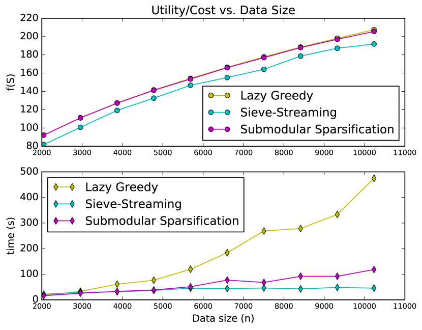
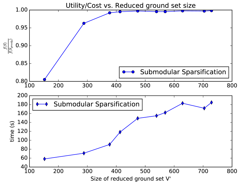
Figure 1 shows how $f(S)$ and time cost varies when we change $n$. The budget size $k$ of the summary set to the number of sentences in a human generated summary. The number of trials in sieve-streaming is $50$, leading to memory requirement of $50k$. The utility curve of SS overlaps that of lazy greedy, while its time cost is much less and increases more slowly than that of lazy greedy. Sieve-streaming performs much worse than SS in terms of utility, and its time cost is only slightly less (this is because it quickly fills $S$ with $k$ elements and stops much earlier before seeing all $n$ elements). Figure 2 shows how relative utility $f(S)/f(S_{greedy})$ ($S_{greedy}$ is the greedy solution) and SS time cost vary with the size of the reduced set $V^{\prime}$. SS quickly reaches a $f(S)=0.97f(S_{greedy})$ once the size exceeds $300$, while its computational cost increases slowly.

4.2 News Summarization

Figure 4: Size of data $n$ vs. time cost on daily news summarization results of $3823$ days’ news from New York Times corpus between 1996-2007. The area of each circle is proportional to the relative utility $f(S)/f(S_{greedy})$.

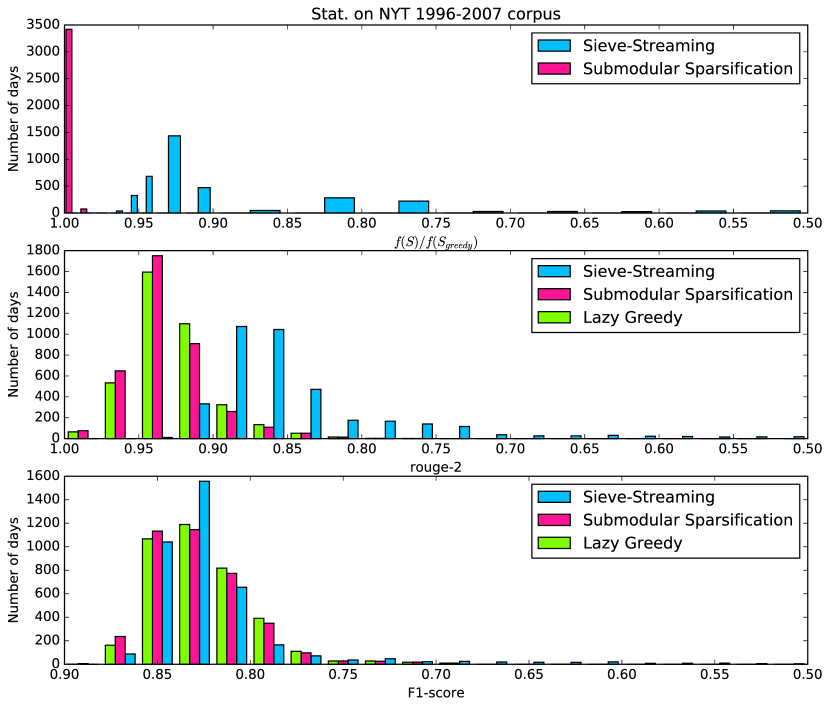
We conduct summarization experiments on two large news corpora, The NYTs annotated corpus 1996-2007 (https://catalog.ldc.upenn.edu/LDC2008T19), and the DUC 2001 corpus (http://www-nlpir.nist.gov/projects/duc). The first dataset includes articles published in the NYTs over $3823$ days from 1996-2007. We collect the sentences in articles associated with human generated summaries as the ground set $V$ (with sizes varying from $2000$ to $20000$), and extract their TFIDF features to build $f(S)$. We concatenate the sentences from all human generated summaries for the same date as a reference summary. We compare the machine generated summaries produced by different methods with the reference summary by ROUGE-2 [18] (recall on 2-grams) and ROUGE-2 F1-score (F1-measure based on recall and precision on 2-grams).

We also compare their relative utility. As before, sieve-streaming has memory set at $50k$. The statistics over $3823$ days are shown in Figure 3. SS has a relative utility of $\geq 0.99$ on most days, while sieve-streaming is mostly in the $[0.92,0.93]$ region. Both the ROUGE-2 and F1 score of SS are better than sieve-streaming, and even outperform greedy a bit. This may be because SS removes many of the elements on which greedy might become trapped in some local sub-optimal region.

Figure 5: Scatter plot of relative utility $f(S)/f(S_{greedy})$ achieved by submodular sparsification on the $3823$ days’ news with the corresponding size of ground set $V$ and the size of reduced set $V^{\prime}$. Each point corresponds to one day.

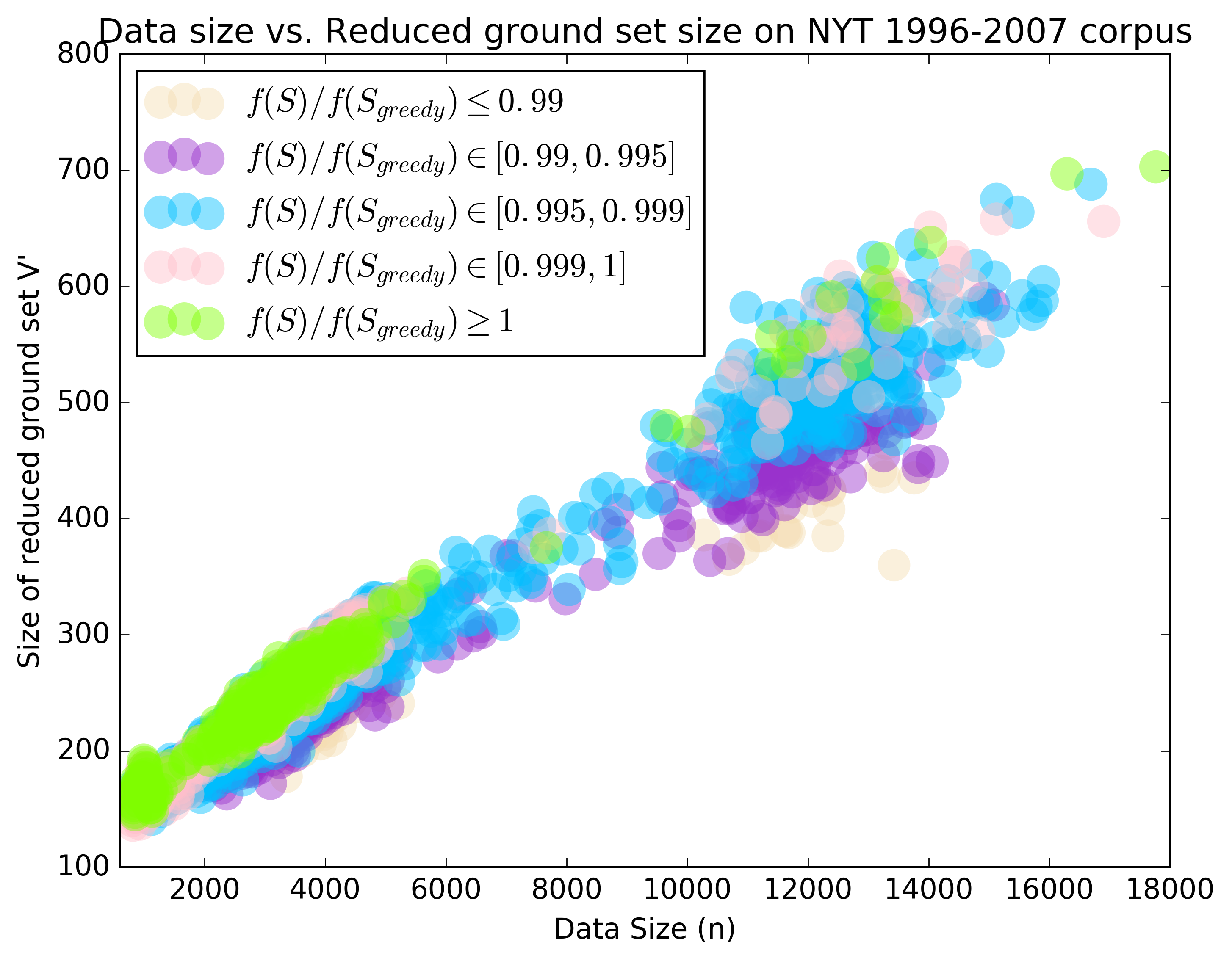
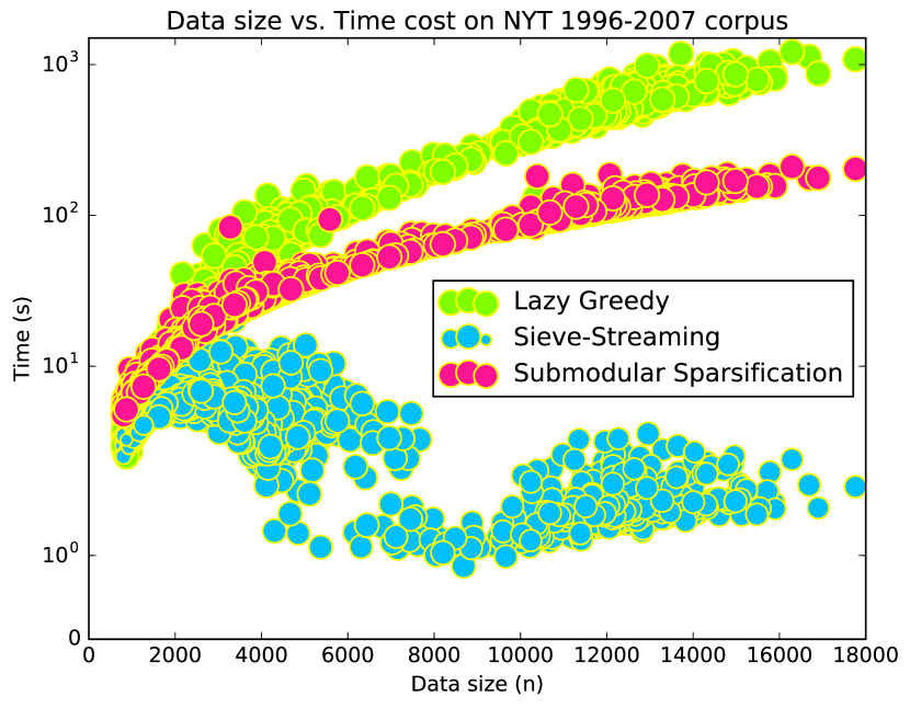
Figure 4 shows the number $n$ of sentences per day and the corresponding time cost of each algorithm. The area of each circle is proportional to relative utility. We use a log scale time axis for a wider dynamic range. SS reduces computation over lazy greedy especially when $n$ is large. Sieve-streaming’s time cost decreases when $n\geq 6000$, but its relative utility is reduced due to the aforementioned early stopping. Figure 5 shows the distribution of relative utility achieved by SS with different data sizes $n$ and reduced ground set sizes over $3823$ different days. The relative utility of SS is $\geq 0.99$ on most days, and even $\geq 1$ when $n\leq 6000$. This indicates that summarization on the reduced set $V^{\prime}$ achieved by SS can even occasionally outperform that on the original ground set $V$.

4.3 Video Summarization

We apply lazy greedy, sieve-streaming, and SS to $25$ videos from dataset SumMe [13] (http://www.vision.ee.ethz.ch/~gyglim/vsum/). Each video has $1000\sim 10000$ frames as given in Table 2 [1]. The results are given in [1]. The greedy algorithm on the SS-reduced ground set consistently approaches or outperforms lazy greedy on recall and F1-score, while the time cost is much smaller and a large fraction of frames may be removed.

5 Appendix

5.1 Proof of Lemma 3

Proof.

Firstly, we have the following inequality.

$$f(x|v) =f(x+u|v)-f(u|v+x)$$

$$=f(x|u+v)+f(u|v)-f(u|v+x)$$

$$\leq f(x|u)+f(u|v)-f(u|v+x).$$ (15)

The first two equalities follow from the definition of marginal gain, while the inequality is due to submodularity. Following the definition of $w_{uv}$ in Eq. (3), we have

$$w_{vx} =f(x|v)-f(v|V-v)$$

$$\leq f(x|u)+f(u|v)-f(u|v+x)-f(v|V-v)$$

$$\leq\left[f(x|u)-f(u|V-u)\right]+\left[f(u|v)-f(v|V-v)\right]$$

$$=w_{ux}+w_{vu}.$$ (16)

The first inequality is due to Eq. (5.1), and the second inequality is via submodularity. ∎

5.2 Proof of Proposition 1

Proof.

Define a set $A_{u}$ for each $u\in V^{\prime}$ such that $A_{u}=\{v\in V:w_{uv}\leq\epsilon\}$. Note $u\in A_{u}$ because $w_{uu}=-f(u|V\backslash u)\leq 0\leq\epsilon$ and hence $V^{\prime}\subseteq\cup_{u\in V^{\prime}}A_{u}$. The objective function $h$ in Eq. (9) can be written as

$$h(V^{\prime}) =\left|\left\{v\in V\backslash V^{\prime}:w_{V^{\prime}v}\leq\epsilon\right\}\right|=\left|\left\{v\in V\backslash V^{\prime}:\exists x\in V^{\prime}:w_{xv}\leq\epsilon\right\}\right|$$ (17)

$$=\left|\left(\bigcup_{u\in V^{\prime}}A_{u}\right)\setminus V^{\prime}\right|=\left|\bigcup_{u\in V^{\prime}}A_{u}\right|-\left|V^{\prime}\right|,$$ (18)

where $f_{SC}(V^{\prime})=\left|\bigcup_{u\in V^{\prime}}A_{u}\right|$ is the simple set cover function [11], which is monotone non-decreasing submodular, and $-|V^{\prime}|$ is a monotone decreasing modular (negative cardinality) function. Because the sum of a submodular function and a modular function is still submodular, the objective in Eq. (9) is non-monotone submodular. ∎

5.3 Proof of Theorem 1

Proof.

Recall that $u^{*}_{v}\in\operatorname*{argmin}_{u\in V^{*}}w_{uv}$ is the tail node of an edge with the minimal weight over all edges from elements in $V^{*}$ to head $v$. Since $|V^{*}|\geq k$, the greedy algorithm on $V^{*}$ will run for $k$ steps and select $k$ elements. We use $S_{i}$ to denote the solution set at the beginning of the $i^{th}$ step, let $u_{i}\in\operatorname*{argmax}_{x\in V^{*}\setminus S_{i}}f(x|S_{i})$ be the selected element in this step. In addition, let $v_{i}=\operatorname*{argmax}_{x\in V\setminus S_{i}}f(x|S_{i})$ be the unfettered greedy choice at step $i$. Then we have the following:

$$\begin{array}[]{ll}f(v_{i}|S_{i})&\leq f(u_{i}|S_{i})+\min\limits_{x\in V^{*}}w_{xv_{i}|S}\\ &\leq f(u_{i}|S_{i})+\min\limits_{x\in V^{*}}w_{xv_{i}}\\ &=f(u_{i}|S_{i})+w_{u^{*}_{v_{i}}v_{i}}\\ &\leq f(u_{i}|S_{i})+\epsilon.\end{array}$$ (19)

The first inequality is by Eq. (8), the second inequality is due to Lemma 1, while the last inequality comes from the definition of problem Eq. (9). Hence, for arbitrary $i$, we have

$$\begin{array}[]{ll}f(S^{*})&\leq f(S_{i}\cup S^{*})\\ &\leq f(S_{i})+\sum\limits_{x\in S^{*}\backslash S_{i}}f(x|S_{i})\\ &\leq f(S_{i})+\sum\limits_{x\in S^{*}}f(x|S_{i})\\ &\leq f(S_{i})+k\max\limits_{x\in V}f(x|S_{i})\\ &=f(S_{i})+kf(v_{i}|S_{i})\\ &\leq f(S_{i})+k\left[f(u_{i}|S_{i})+\epsilon\right]\\ &=f(S_{i})+k\left[f(S_{i+1})-f(S_{i})+\epsilon\right].\end{array}$$ (20)

The first inequality uses monotonicity of $f(\cdot)$, while the second one is due to submodularity. The third inequality is due to the non-negativity of $f(\cdot)$. The fourth inequality is due to the maximal greedy selection rule for the greedy algorithm on the original ground set $V$. The fifth inequality is the result of applying Eq. (19). The last equality is due to the greedy selection rule $S_{i+1}=u_{i}\cup S_{i}$ for the greedy algorithm on the reduced ground set $V^{*}$. Rearranging Eq. (20) yields

$$[f(S^{*})-k\epsilon]-f(S_{i})\leq k[f(S_{i+1})-f(S_{i})]$$ (21)

Let

$$\delta_{i}=[f(S^{*})-k\epsilon]-f(S_{i}),$$ (22)

then the rearranged inequality equals to

$$\delta_{i}\leq k[\delta_{i}-\delta_{i+1}],$$ (23)

Since $\delta_{i}-\delta_{i+1}\geq 0$, this equals to

$$\delta_{i+1}\leq\left(1-\frac{1}{k}\right)\delta_{i}.$$ (24)

Since in total $k$ elements are selected by the greedy algorithm, applying Eq. (24) from $i=0$ to $i=k$ yields

$$\delta_{k}\leq\left(1-\frac{1}{k}\right)^{k}\delta_{0}\leq e^{-1}\delta_{0}.$$ (25)

By using the definition of $\delta_{i}$ in Eq. (22), the above inequality leads to

$$f(S^{\prime})=f(S_{k})\geq\left(1-e^{-1}\right)\left(f(S^{*})-k\epsilon\right).$$ (26)

This completes the proof. ∎

5.4 Proof of Lemma 4

Proof.

The proof follows from Lemma 3 and our assumption to $u$.

$$w_{uv}\leq w_{uu^{*}_{v}}+w_{u^{*}_{v}v}$$

$$= f(v|u^{*}_{v})+f(u^{*}_{v}|u)-f(u^{*}_{v}|V\backslash u^{*}_{v})-f(u|V\backslash u)$$

$$= f(v+u^{*}_{v})+f(u+u^{*}_{v})-f(u^{*}_{v})-f(u)$$

$$-f(u^{*}_{v}|V\backslash u^{*}_{v})-f(u|V\backslash u)$$

$$\leq 2f(v+u^{*}_{v})-f(u^{*}_{v})-f(u)$$

$$-f(u^{*}_{v}|V\backslash u^{*}_{v})-f(u|V\backslash u)$$

$$= 2\left[f(v|u^{*}_{v})-f(u^{*}_{v}|V\backslash u^{*}_{v})\right]$$

$$+\left[f(u^{*}_{v})+f(u^{*}_{v}|V\backslash u^{*}_{v})-f(u)-f(u|V\backslash u)\right]$$

$$\leq 2w_{u^{*}_{v}v}.$$

The first inequality is due to Lemma 3. The second inequality is because $f(u+u^{*}_{v})\leq f(v+u^{*}_{v})$ which follows from $u\in P(u^{*}_{v})$. The third inequality is due to $u\in Q(u^{*}_{v})$. ∎

5.5 Proof of Proposition 2

Proof.

Recall $V^{*}$ is the optimal solution of problem in Eq. (9). Due to the definition of $|V|/(8K)$-NN ball, we have

$$\forall v\in V_{u^{*}}\backslash B\left(u^{*},|V|/(8K)\right),f(u+u^{*})\leq f(v+u^{*}).$$ (27)

Hence, $u\in P(u^{*}_{v})\cap Q(u^{*}_{v})$. By using Lemma 4, we have

$$w_{uv}\leq 2w_{u^{*}v}.$$ (28)

This completes the proof. ∎

5.6 Proof of Proposition 3

Proof.

According to Proposition 2, for each $u^{*}\in V^{*}$, if one $u\in B\left(u^{*},|V|/(cK)\right)\cap Q(u^{*})$ is sampled into $U$ in some iteration of Algorithm 1, then any item $v$ outside the ball satisfies

$$w_{Uv} =\min_{x\in U}w_{xv}\leq w_{uv}$$

$$\leq 2w_{u^{*}_{v}v}=2w_{V^{*}v}.$$

Hence, one element $u$ fulfilling $w_{Uu}\geq 2w_{V^{*}u}$ in the complement set must be contained in least one of the $K$ $|V|/(cK)$-NN balls whose centers are the $K$ elements in $V^{*}$. Therefore, the total number of such $u$ is at most $|V|/c=K\times|V|/(cK)$, the maximal number of elements in all the $K$ $|V|/(cK)$-NN balls. ∎

5.7 Proof of Proposition 4

Proof.

We consider $V_{i}$, set $V$ at the beginning of the $i^{th}$ iteration, and $V_{i-1}$, set $V$ right before the removal step of the previous iteration. According to the pruning amount $1-1/\sqrt{c}$:

$$|V_{i}|=1/\sqrt{c}|V_{i-1}|.$$ (29)

Since Proposition 3 indicates

$$\left|\{u\in V_{i}:w_{Uu}\geq 2w_{V^{*}u}\}\right|\leq\frac{|V_{i-1}|}{c},$$ (30)

we have

$$\left|\{v\in V_{i}:w_{Uv}\leq 2w_{V^{*}v}\}\right|$$

$$= |V_{i}|-\left|\{u\in V_{i}:w_{Uu}\geq 2w_{V^{*}u}\}\right|$$

$$\geq \frac{1}{\sqrt{c}}|V_{i-1}|-\frac{1}{c}|V_{i-1}|$$

$$= \left(1-\frac{1}{\sqrt{c}}\right)\times(\frac{1}{\sqrt{c}})|V_{i-1}|$$

$$= \left(1-\frac{1}{\sqrt{c}}\right)|V_{i}|.$$

Because the above result is correct for arbitrary $i$, it completes the proof. ∎

5.8 Proof of Lemma 5

Proof.

According to Proposition 4, after removal, all the elements in $\{v\in V:w_{Uv}>2w_{V^{*}v}\}$ are retained in $V^{\prime}$. So none of them is in $V\backslash V^{\prime}$.

According to Proposition 2, if for each $u^{*}\in V^{*}$ at least one alternate $u\in B\left(u^{*},|V|/(cK)\right)\cap Q(u^{*})$ is sampled and added into $U$, $\forall v\in V$, we have $w_{V^{\prime}v}\leq 2w_{V^{*}v}$. This completes the proof. ∎

5.9 Proof of Proposition 5

Proof.

According to the assumption and definition of $Q(u^{*})$ in Lemma 4, $\forall u\in U$,

$$\Pr\left(u\in Q(u^{*})\right)\geq q.$$ (31)

In addition, the probability for that an uniform sample $u$ is inside the $|V|/(cK)$-NN ball $B\left(u^{*},|V|/(cK)\right)$ of $u^{*}$ is

$$\Pr\left(u\in B\left(u^{*},|V|/(cK)\right)\right)=\frac{1}{cK}.$$ (32)

Combining the two probabilities, we have

$$\Pr\left(u\not\in B\left(u^{*},|V|/(cK)\right)\cap Q(u^{*})\right)\leq 1-\frac{q}{cK}.$$ (33)

Since $r=O(cK)=pcK$, among the $r\log n=pcK\log n$ samples of $U$ in one iteration, for one specific $u^{*}$, the probability that no sample belongs to $B\left(u^{*},|V|/(8K)\right)\cap Q(u^{*})$ is

$$\Pr \left(U\cap\left(B\left(u^{*},|V|/(8K)\right)\cap Q(u^{*})\right)=\emptyset\right)$$

$$\leq\left(1-\frac{q}{cK}\right)^{r}=\left(1-\frac{q}{cK}\right)^{pcK\log n}\leq n^{-qp}.$$

Note there are $K$ items in $V^{*}$, and there will be at most $\log_{\sqrt{c}}n$ iterations. By union bound, the failure probability that no $u\in B(u^{*},|V|/(cK))\cap Q(u^{*})$ is sampled and added into $U$ for at least one $u^{*}\in V^{*}$ in at least one iteration of Algorithm 1 is at most

$$K\times n^{-qp}\times\log_{\sqrt{c}}n\leq n^{1-qp}\log_{\sqrt{c}}n.$$ (34)

∎

5.10 Proof of Theorem 1

Proof.

Firstly, since $r\log n=pcK\log n$ elements are selected into $V^{\prime}$ per iteration, and the number of iterations is $\log_{\sqrt{c}}n$, so the size of $V^{\prime}$ is

$$|V^{\prime}|=pcK\log n\times\log_{\sqrt{c}}n=(pc/\log_{\sqrt{c}})K\log^{2}n.$$ (35)

Secondly, combing the results of Lemma 5 and failure probability $n^{1-qp}\log_{\sqrt{c}}n$ in Proposition 5, we have: with success probability $1-n^{1-qp}\log_{\sqrt{c}}n$, $\forall v\in V\backslash V^{\prime}$, $w_{V^{\prime}v}\leq 2w_{V^{*}v}$.

Thirdly, since $w_{V^{\prime}v}\leq 2w_{V^{*}v}$, we replace $w_{u^{*}_{v_{i}}v_{i}}$ with $2w_{u^{*}_{v_{i}}v_{i}}$ in Eq. (19), the rest proof of Theorem 1 leads to

$$f(S^{\prime})\geq\left(1-e^{-1}\right)\left(f(S^{*})-2k\epsilon\right).$$ (36)

This completes the proof. ∎

5.11 Experiments on DUC2001 News Summarization

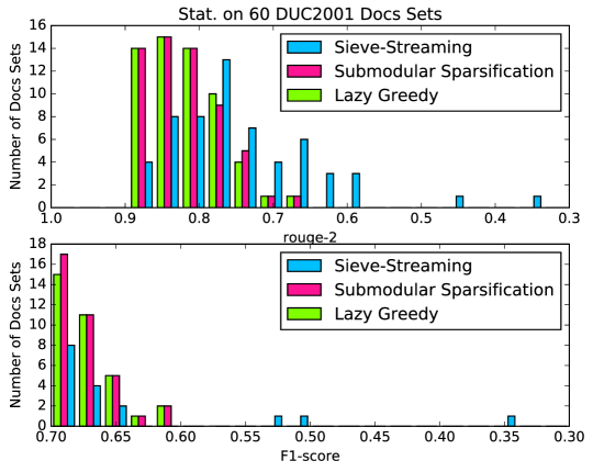
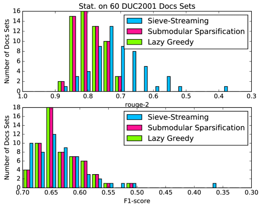
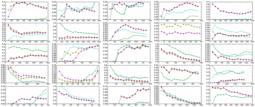
We also observe similar result on DUC 2001 corpus, which are composed of two datasets. The first one includes $60$ sets of documents, each is selected by a NIST assessor because the documents in a set are related to a same topic. The assessor also provides four human generated summary of word count $400,200,100,50$ for each set. In Figure 6 and Figure 7, we report the statistics to ROUGE-2 and F1-score of summaries of the same size generated by different algorithms. The second dataset is composed of four document sets associated with four topics. We report the detailed results in Table 1. Both of them show submodular sparsification can achieve similar performance as greedy algorithm, whereas outperforms sieve-streaming.

Figure 6: Statistics of relative utility $f(S)/f(S_{greedy})$, ROUGE-2 score and F1-score on topic based news summarization results of $60$ document sets from DUC2001 training and test set, comparing to $400$-word human generated summary.

Figure 7: Statistics of relative utility $f(S)/f(S_{greedy})$, ROUGE-2 score and F1-score on topic based news summarization results of $60$ document sets from DUC2001 training and test set, comparing to $200$-word human generated summary.

Table 1: Performance of Lazy greed, sieve-streaming, and submodular sparsification on four topic summarization datasets from DUC 2001. For each topic, the machine generated summary is compared to four human generated ones of word count from 50 to 400.

Algorithm	words	Daycare		Healthcare		Pres92		Robert Gates
		ROUGE2	F1	ROUGE2	F1	ROUGE2	F1	ROUGE2	F1
Lazy Greedy	400	$0.836$	$0.674$	$0.845$	$0.686$	$0.885$	$0.686$	$0.849$	$0.734$
	200	$0.813$	$0.615$	$0.811$	$0.632$	$0.842$	$0.623$	$0.788$	$0.682$
	100	$0.766$	$0.542$	$0.753$	$0.605$	$0.618$	$0.420$	$0.715$	$0.621$
	50	$0.674$	$0.484$	$0.765$	$0.539$	$0.602$	$0.341$	$0.631$	$0.514$
Sieve-Streaming	400	$0.825$	$0.687$	$0.814$	$0.711$	$0.827$	$0.710$	$0.798$	$0.745$
	200	$0.789$	$0.627$	$0.782$	$0.675$	$0.670$	$0.659$	$0.691$	$0.688$
	100	$0.747$	$0.542$	$0.658$	$0.597$	$0.414$	$0.443$	$0.632$	$0.620$
	50	$0.607$	$0.475$	$0.681$	$0.551$	$0.413$	$0.345$	$0.553$	$0.477$
SS	400	$0.837$	$0.674$	$0.845$	$0.686$	$0.883$	$0.685$	$0.849$	$0.734$
	200	$0.813$	$0.615$	$0.811$	$0.632$	$0.842$	$0.623$	$0.788$	$0.682$
	100	$0.766$	$0.542$	$0.753$	$0.605$	$0.617$	$0.420$	$0.715$	$0.621$
	50	$0.674$	$0.484$	$0.765$	$0.539$	$0.602$	$0.341$	$0.631$	$0.514$

5.12 Experiments on Video Summarization

5.13 Video Summarization

We apply lazy greedy, sieve-streaming, and SS to $25$ videos from video summarization dataset SumMe [13]. Each video has $1000\sim 10000$ frames as given in Table 2.

We resize each frame to a $180\times 360$ image, and extract features from two standard image descriptors, i.e., a pyramid of HoG (pHoG) [5] to delineate local and global shape, and GIST [25] to capture global scene. The $2728$ pHoG features are achieved over a four-level pyramid using $8$ bins with angle of $360$ degrees. The $256$ GIST features are obtained by using $4\times 4$ blocks and $8$ orientation per scale. We concatenate them to form a $2984$-dimensional feature vector for each frame to build $f(\cdot)$. Each algorithm selects $15\%$ of all frames as summary set, i.e., $k=0.15|V|$. Sieve-streaming holds a memory of $10k$ frames.

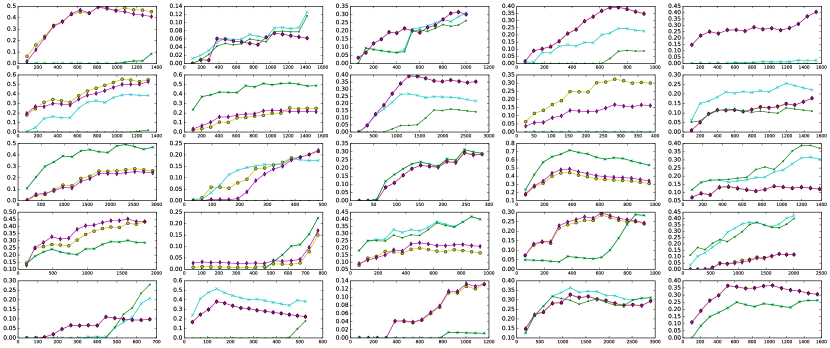
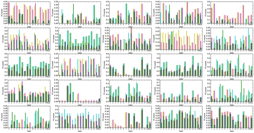
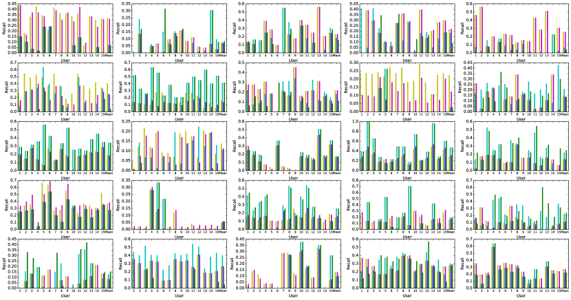
We compare the summaries generated by the three algorithms with the ones produced by the ground truth and $15$ users. Each user was asked to select a subset of frames as summary, and ground truth score of each frame is given by voting from all $15$ users. For each video, we compare each algorithm generated summary with the reference summary composed of the top $p$ frames with the largest ground truth scores for different $p$, and the user summary from different users. In particular, we report F1-score and recall for comparison to ground truth score generated summaries in Figure 8 and Figure 9. We report F1-score and recall for comparison to user summaries in Figure 10 and Figure 11. In each plot for each video, we also report the average F1-score and average recall over all $15$ users.

SS consistently approaches or outperforms lazy greedy, while the time cost is much smaller according to Table 2 [1]. Although on a few videos sieve-streaming achieves the best F1-score, in these cases its generated summaries are trivially dominated by the first $15\%$ frames as shown in Figure 8-11.

Figure 8: F1-score of the summaries generated by lazy greedy (“$\bullet$”), sieve-streaming ( “$\times$”), submodular sparsification (“$\blacklozenge$”) and the first $15\%$ frames (“$\cdot$”) comparing to reference summaries of different sizes between $[0.02|V|,0.32|V|]$ based on ground truth score (voting from $15$ users) on $25$ videos from SumMe. Each plot associates with a video.

Figure 9: Recall of the summaries generated by lazy greedy (“$\bullet$”), sieve-streaming ( “$\times$”), submodular sparsification (“$\blacklozenge$”) and the first $15\%$ frames (“$\cdot$”) comparing to reference summaries of different sizes between $[0.02|V|,0.32|V|]$ based on ground truth score (voting from $15$ users) on $25$ videos from SumMe. Each plot associates with a video.

Figure 10: F1-score of the summaries generated by greedy (yellow bar), sieve-streaming ( cyan bar), SS (magenta bar) and the first $15\%$ frames (green bar) comparing to reference summaries from $15$ users on $25$ videos from SumMe dataset. Each plot associates with a video.

Figure 11: Recall of the summaries generated by greedy (yellow bar), sieve-streaming ( cyan bar), SS (magenta bar) and the first $15\%$ frames (green bar) comparing to reference summaries from $15$ users on $25$ videos from SumMe dataset. Each plot associates with a video.

Table 2: Information of SumMe dataset and time cost (CPU seconds) of different algorithms.

Video	#frames	$|V^{\prime}|$	Lazy Greedy	Sieve-streaming	SS
Air Force One	4494	1031	907.3712	3.9182	71.4521
Base jumping	4729	1074	164.1434	5.5865	84.6877
Bearpark climbing	3341	1038	177.8583	3.7311	48.0415
Bike polo	3064	866	96.5305	3.9578	36.4832
Bus in rock tunnel	5131	1387	505.7766	6.0088	125.8121
Car over camera	4382	1396	146.9416	5.3323	69.6157
Car railcrossing	5075	1210	852.1686	5.2265	96.2396
Cockpit landing	9046	2292	669.8063	12.3186	212.7866
Cooking	1286	200	30.0717	1.2868	5.7096
Eiffel tower	4971	1647	304.2690	5.4755	86.5552
Excavators river crossing	9721	1971	1507.3028	13.8139	284.5136
Fire Domino	1612	464	34.2871	1.8814	9.9833
Jumps	950	308	15.0508	0.9055	4.8719
Kids playing in leaves	3187	986	221.4644	3.4660	41.1956
Notre Dame	4608	1136	169.1235	5.1406	72.9076
Paintball	6096	1664	763.3255	6.7853	128.1723
Paluma jump	2574	727	210.8670	2.5342	26.7430
Playing ball	3120	697	132.7437	3.2250	32.3198
Playing on water slide	3065	778	111.7358	3.4088	30.4131
Saving dolphines	6683	1860	435.0732	7.3322	121.5891
Scuba	2221	775	45.6177	2.5213	18.4227
St Maarten Landing	1751	628	19.0717	2.8701	12.4074
Statue of Liberty	3863	1223	160.7075	4.0164	55.7420
Uncut evening flight	9672	3324	718.7015	14.6717	208.8540
Valparaiso downhill	5178	1438	428.3941	6.0002	154.5902

References

- [1] Anonymous. Supplementary material for submodular sparsification. In Submitted to NIPS, 2016.
- [2] Ashwinkumar Badanidiyuru, Baharan Mirzasoleiman, Amin Karbasi, and Andreas Krause. Streaming submodular maximization: Massive data summarization on the fly. In SIGKDD, pages 671–680, 2014.
- [3] Ashwinkumar Badanidiyuru and Jan Vondrák. Fast algorithms for maximizing submodular functions. In SODA, pages 1497–1514, 2014.
- [4] Mohammadhossein Bateni, Mohammadtaghi Hajiaghayi, and Morteza Zadimoghaddam. Submodular secretary problem and extensions. ACM Trans. Algorithms, 9(4):32:1–32:23, 2013.
- [5] Anna Bosch, Andrew Zisserman, and Xavier Munoz. Representing shape with a spatial pyramid kernel. In ACM International Conference on Image and Video Retrieval, pages 401–408, 2007.
- [6] Niv Buchbinder, Moran Feldman, Joseph (Seffi) Naor, and Roy Schwartz. A tight linear time (1/2)-approximation for unconstrained submodular maximization. In FOCS, pages 649–658, 2012.
- [7] Niv Buchbinder, Moran Feldman, Joseph (Seffi) Naor, and Roy Schwartz. Submodular maximization with cardinality constraints. In SODA, pages 1433–1452, 2014.
- [8] Niv Buchbinder, Moran Feldman, and Roy Schwartz. Online submodular maximization with preemption. In SODA, pages 1202–1216, 2015.
- [9] Chandra Chekuri, Shalmoli Gupta, and Kent Quanrud. Streaming algorithms for submodular function maximization. arXiv:1504.08024, 2015.
- [10] Dan Feldman, Amos Fiat, Micha Sharir, and Danny Segev. Bi-criteria linear-time approximations for generalized k-mean/median/center. In Proceedings of the Twenty-third Annual Symposium on Computational Geometry, pages 19–26, 2007.
- [11] Satoru Fujishige. Submodular functions and optimization. Annals of discrete mathematics. Elsevier, 2005.
- [12] Ryan Gomes and Andreas Krause. Budgeted nonparametric learning from data streams. In ICML, 2010.
- [13] Michael Gygli, Helmut Grabner, Hayko Riemenschneider, and Luc Van Gool. Creating summaries from user videos. In ECCV, 2014.
- [14] Piotr Indyk, Sepideh Mahabadi, Mohammad Mahdian, and Vahab S. Mirrokni. Composable core-sets for diversity and coverage maximization. In PODS, pages 100–108, 2014.
- [15] Rishabh Iyer, Stefanie Jegelka, and Jeff Bilmes. Curvature and optimal algorithms for learning and minimizing submodular functions. In NIPS, 2013.
- [16] Rishabh Iyer, Stefanie Jegelka, and Jeff A. Bilmes. Fast semidifferential-based submodular function optimization. In ICML, 2013.
- [17] Jure Leskovec, Andreas Krause, Carlos Guestrin, Christos Faloutsos, Jeanne VanBriesen, and Natalie Glance. Cost-effective outbreak detection in networks. In SIGKDD, pages 420–429, 2007.
- [18] Chin-Yew Lin. Rouge: A package for automatic evaluation of summaries. In Text Summarization Branches Out: Proceedings of the ACL-04 Workshop, pages 74–81, 2004.
- [19] Hui Lin and Jeff Bilmes. A class of submodular functions for document summarization. In ACL, pages 510–520, 2011.
- [20] Michel Minoux. Accelerated greedy algorithms for maximizing submodular set functions. In Optimization Techniques, volume 7 of Lecture Notes in Control and Information Sciences, chapter 27, pages 234–243. 1978.
- [21] Vahab Mirrokni and Morteza Zadimoghaddam. Randomized composable core-sets for distributed submodular maximization. In STOC, pages 153–162, 2015.
- [22] Baharan Mirzasoleiman, Ashwinkumar Badanidiyuru, Amin Karbasi, Jan Vondrák, and Andreas Krause. Lazier than lazy greedy. In AAAI, pages 1812–1818, 2015.
- [23] Baharan Mirzasoleiman, Amin Karbasi, Rik Sarkar, and Andreas Krause. Distributed submodular maximization: Identifying representative elements in massive data. In NIPS, pages 2049–2057, 2013.
- [24] G. L. Nemhauser, L. A. Wolsey, and M. L. Fisher. An analysis of approximations for maximizing submodular set functions—I. Mathematical Programming, 14(1):265–294, 1978.
- [25] Aude Oliva and Antonio Torralba. Modeling the shape of the scene: A holistic representation of the spatial envelope. International Journal of Computer Vision, 42(3):145–175, 2001.
- [26] Xinghao Pan, Stefanie Jegelka, Joseph E Gonzalez, Joseph K Bradley, and Michael I Jordan. Parallel double greedy submodular maximization. In NIPS, pages 118–126, 2014.
- [27] Kai Wei, Rishabh Iyer, and Jeff Bilmes. Fast multi-stage submodular maximization. In ICML, 2014.