Baryon transition form factors at the pole

Abstract

Electromagnetic resonance properties are uniquely defined at the pole and do not depend on the separation of the resonance from background or the decay channel. Photon-nucleon branching ratios are nowadays often quoted at the pole, and we generalize the considerations to the case of virtual photons. We derive and compare relations for nucleon to baryon transition form factors both for the Breit-Wigner and the pole positions. Using the MAID2007 and SAID SM08 partial wave analyses of pion electroproduction data, we compare the $G_{M}$, $G_{E}$, and $G_{C}$ form factors for the $\Delta(1232)$ resonance excitation at the Breit-Wigner resonance and pole positions up to $Q^{2}=5$ GeV². We also explore the $E/M$ and $S/M$ ratios as functions of $Q^{2}$. For pole and residue extraction, we apply the Laurent + Pietarinen method.

I Introduction

As baryon resonance properties, evaluated at the pole position, are now beginning to supersede and replace quantities that historically have been determined using Breit-Wigner (BW) plus background parameterizations, we extend a recent study Workman:2013rca of photo-decay couplings at the pole to the regime of non-zero $Q^{2}$. The shift to pole-related quantities is reflected in the Review of Particle Properties (RPP) pdg , with many pole values coming from the Bonn-Gatchina multi-channel analyses bnga . Some plots of transition form factors at the BW position, as a function of photon virtuality, are now also available in the RPP.

Calculations at the pole are, in principle, well-defined and less model-dependent than the BW approach. However, the continuation of fit amplitudes to the pole is itself a possible source of error. With the aim to minimize model dependence of the pole extraction procedure this uncertainty has motivated numerous studies involving speed plots, regularization methods, contour integration Doring:2009yv ; ceci11 ; masj11 ; yang11 ; tiat10 ; suzu10 , and the most recent Laurent series representations (L+P) based on separation of pole and regular part, and using the conformal mapping variable to expand the regular part in power series svar12 .

While analysis in terms of BW amplitudes is more in line with the early fits, based on simple BW plus background parameterizations, fits done within dynamical models are more naturally presented in terms of poles Kamano:2013iva ; Ronchen:2015vfa ; Ronchen:2014cna . In the chiral effective field theory calculation of Ref. Gail , for example, complex form factor results at the pole could only be compared to real BW values coming from fits to data. See also Refs. Pascalutsa:2005vq ; Bernard:2005fy for related results. Also, in chiral unitary resonance dynamics, there is no genuine resonance seed that would allow for the definition of a meaningful, purely real helicity coupling Jido:2007sm ; Doring:2010rd ; Doring:2007rz . As a result, ad-hoc prescriptions were used to translate these results to quoted real BW helicity amplitudes. A proper comparison, however, requires the associated quantities extracted at the pole of amplitudes obtained from fits to experimental data.

To achieve this goal, we have extracted pole parameters with the L+P method from two energy-dependent (ED) partial wave analyses, MAID and SAID, which are fitted to the world data base of pion electroproduction. The differences observed by this comparison will give an insight of the uncertainty of the pole form factors due to the differences in the MAID and SAID techniques and consequently also to the experimental database.

For the $\Delta(1232)$ state, considerable attention Aznauryan:2016wwm ; Ramalho:2015qna ; aznauryan1 ; segovia ; Segovia:2013uga ; Ronniger:2012xp ; Sanchis-Alepuz:2013iia ; Ramalho:2012ng ; Santopinto:2012nq ; Aznauryan:2011qj ; Santopinto:2010zz ; ebac ; ungaro ; Fiolhais:1996bp has been addressed to the $Q^{2}$ evolution of amplitudes, as well as differences in the $Q^{2}$ dependence of bare couplings, within models, and meson-cloud contributions. For a review, see, e.g., Ref. Pascalutsa:2006up . Transition form factors are now also determined in lattice QCD simulations Alexandrou:2013ata ; Alexandrou:2010uk . Here, the quark masses are so large that the $\Delta(1232)$ appears as a bound state, but it has been realized in Ref. Agadjanov:2014kha that in future simulations, close to the physical point, the finite resonance width will complicate the extraction. Therefore, in Ref. Agadjanov:2014kha a method has been proposed to determine transition form factors at the pole. This stresses again the relevance of providing pole values for existing phenomenological analyses, which is the aim of this study.

The main focus of this paper is the $\Delta(1232)$ virtual-photon decay amplitudes and related transition form factors. As the amplitudes themselves become infinite at the pole, we are interested in residues. The connection between multipole residues and the photo-decay amplitudes has been clarified in a previous paper Workman:2013rca and in the Note on N and Delta Resonance mini-reviews of the 2012 and 2014 PDG listings pdg .

Here we will compare BW and pole extractions, using the MAID2007 and SAID SM08 partial wave analyses of pion electroproduction data, utilizing the recent Laurent + Pietarinen (L+P) pole extraction method L+P2013 ; L+P2014 ; L+P2014a ; L+P2015 ; L+P2016 which has proven to be a precise and very reliable tool for the determination of pole positions and residues.

The $\Delta(1232)$ E/M and S/M ratios have been studied for many decades. Interest in the E/M ratio, for real-photon interactions, was largely motivated by the fact that, in a simple non-relativistic quark model, this ratio would be zero bm and, thus, deviations from zero would require more complicated interactions. The measured value of this ratio was small pdg , $-2.5\pm 0.5\%$, but its precise value varied as photoproduction cross sections and beam-asymmetry $\Sigma$ measurements became more precise. The prediction for this ratio, at very large $Q^{2}$ from pQCD carlson , has been more difficult to confirm. The ratio is predicted to become unity, whereas, at the real-photon point, it is small and negative. The variation of this ratio with $Q^{2}$ has also changed significantly as electroproduction data have improved.

In Section II, we first give definitions of the standard BW quantities and then define the associated pole-valued results we will be considering. In Section III, we then give a brief overview of the BW and pole behavior of the $\Delta(1232)$ amplitudes, which are constrained by Watson’s theorem. The L+P fit is described in Section IV and compared to results from a fit, generalized to non-zero $Q^{2}$, described in Ref. Workman:2013rca . Finally, in Section IV, we summarize our findings and prospects for future work.

II Breit-Wigner versus pole quantities

The total cross section of pion electroproduction can be written as a semi-inclusive electron scattering cross section

$$\frac{d\sigma}{d\Omega_{e}dE_{f}}=\Gamma_{V}(\sigma_{T}+\varepsilon\sigma_{L})$$ (1)

with the virtual-photon flux factor

$$\Gamma_{V}=\frac{\alpha}{2\pi^{2}}\frac{E_{f}}{E_{i}}\frac{\kappa_{\ell}}{Q^{2}}\frac{1}{1-\varepsilon}\,,$$ (2)

where $E_{i}$ and $E_{f}$ are the initial and final electron energies in the lab frame, the virtual-photon polarization $\varepsilon$ and the total transverse and longitudinal virtual-photon cross sections

$$\sigma_{T} = \frac{1}{2}(\sigma_{T}^{1/2}+\sigma_{T}^{3/2})\,,$$ (3)

$$\sigma_{T}^{h} = 4\pi\frac{q}{\kappa_{c}}\sum_{\alpha(\ell,J,I)}(2J+1)\,|\mathcal{A}_{\alpha}^{h}|^{2}\;C^{2}\,,$$ (4)

$$\sigma_{L} = 4\pi\frac{q}{\kappa_{c}}\frac{Q^{2}}{k^{2}}\sum_{\alpha(\ell,J,I)}(2J+1)\,|\mathcal{S}_{\alpha}^{1/2}|^{2}\;C^{2}\,,$$ (5)

with $q$ and $k$ being the center-of-mass pion and photon momenta and $\kappa_{l}=(W^{2}-m_{N}^{2})/2m_{N}$ and $\kappa_{c}=(W^{2}-m_{N}^{2})/2W$ the so-called equivalent real photon energies in the lab and c.m. frames. The factor $C$ is $\sqrt{2/3}$ for isospin $3/2$ and $-\sqrt{3}$ for isospin $1/2$. The helicity multipoles are given in terms of electric, magnetic and longitudinal (time-like) multipoles

$$\mathcal{A}_{\ell+}^{1/2} = -{1\over 2}\left[(\ell+2){E}_{\ell+}+\ell{M}_{\ell+}\right],$$ (6)

$$\mathcal{A}_{\ell+}^{3/2} = {1\over 2}\sqrt{\ell(\ell+2)}\left[{E}_{\ell+}-{M}_{\ell+}\right],$$ (7)

$$\mathcal{S}_{\ell+}^{1/2} = -{\ell+1\over\sqrt{2}}{S}_{\ell+}\,,$$ (8)

$$\mathcal{A}_{(\ell+1)-}^{1/2} = -{1\over 2}\left[\ell{E}_{(\ell+1)-}-(\ell+2){M}_{(\ell+1)-}\right],$$ (9)

$$\mathcal{A}_{(\ell+1)-}^{3/2} = -{1\over 2}\sqrt{\ell(\ell+2)}\left[{E}_{(\ell+1)-}+{M}_{(\ell+1)-}\right],$$ (10)

$$\mathcal{S}_{(\ell+1)-}^{1/2} = -{\ell+1\over\sqrt{2}}{S}_{(\ell+1)-}\,,$$ (11)

with $J=\ell+1/2$ for ’$+$’ multipoles and $J=(\ell+1)-1/2$ for ’$-$’ multipoles, all having the same total spin $J$.

In analogy to photoproduction Workman:2013rca , we define the virtual-photon decay amplitudes

$$A_{h}^{BW} = C\,\sqrt{\frac{q_{r}}{\kappa_{r}}\frac{\pi(2J+1)M_{r}\Gamma_{r}^{2}}{m_{N}\Gamma_{\pi,r}}}\;\tilde{\mathcal{A}}_{\alpha}^{h}\,,$$ (12)

$$S_{1/2}^{BW} = C\,\sqrt{\frac{q_{r}}{\kappa_{r}}\frac{\pi(2J+1)M_{r}\Gamma_{r}^{2}}{m_{N}\Gamma_{\pi,r}}}\;\tilde{\mathcal{S}}_{\alpha}^{1/2}\,,$$ (13)

where $\tilde{\mathcal{A}}_{\alpha}^{1/2}$, $\tilde{\mathcal{A}}_{\alpha}^{3/2}$, and $\tilde{\mathcal{S}}_{\alpha}^{1/2}$ are the imaginary parts of the resonance amplitudes at the BW position $W_{r}=M_{r}$.

Similarly, we define the virtual-photon amplitudes at the pole position

$$A_{h}^{pole} = C\,\sqrt{\frac{q_{p}}{\kappa_{p}}\frac{2\pi(2J+1)W_{p}}{m_{N}Res_{\pi N}}}\;\mbox{Res}\,\mathcal{A}_{\alpha}^{h}\,,$$ (14)

$$S_{1/2}^{pole} = C\,\sqrt{\frac{q_{p}}{\kappa_{p}}\frac{2\pi(2J+1)W_{p}}{m_{N}Res_{\pi N}}}\;\mbox{Res}\,\mathcal{S}_{\alpha}^{1/2}\,.$$ (15)

where the subscript $p$ denotes quantities evaluated at the pole position.

The photon momenta, $\kappa_{r}$ and $\kappa_{p}$, are photon equivalent energies and can be written as virtual-photon momenta at $Q^{2}=0$. The amplitudes, $\mathcal{A}_{\alpha}^{h}$ and $\mathcal{S}_{\alpha}^{1/2}$, as well as the residues, $A_{h}^{pole}$ and $S_{1/2}^{pole}$, are functions of the photon virtuality $Q^{2}$.

Through linear combinations, the helicity form factors can also be related to electric, magnetic and charge form factors. These so-called Sachs form factors, $G_{E}^{*}$, $G_{M}^{*}$, and $G_{C}^{*}$, are usually given in two different conventions by Ash Ash67 and by Jones and Scadron Jon73 . Both are related by a square-root factor, $G_{JS}(Q^{2})=G_{Ash}(Q^{2})\times\sqrt{1+Q^{2}/(m_{N}+M_{r})^{2}}$.

Here we will concentrate on the $\Delta(1232)$ transition form factors and give the corresponding expressions. For transitions with different spin and parity, similar relations can be found, see Devenish:1975jd ; Tiator:2011pw .

For the $\gamma N\Delta$ transition, Jones and Scadron Jon73 give the following relations between the total cross sections and the Sachs form factors:

$$\sigma_{T}+\varepsilon\sigma_{L} = \frac{2\pi\alpha}{\Gamma_{r}m_{N}^{2}}\frac{k_{r}(Q^{2})^{2}}{\kappa_{r}(1+Q^{2}/(m_{N}+M_{\Delta})^{2}}$$

$$({G_{M}^{*}}^{2}(Q^{2})+3{G_{E}^{*}}^{2}(Q^{2})+\varepsilon\frac{Q^{2}}{4M_{\Delta}^{2}}{G_{C}^{*}}^{2}(Q^{2}))\,.$$

In the convention of Ash, the Sachs form factors take the form

$$G_{M}^{*}(Q^{2}) =-c_{\Delta}(A_{1/2}+\sqrt{3}A_{3/2})\,,$$ (17)

$$G_{E}^{*}(Q^{2}) =\,\,\,c_{\Delta}(A_{1/2}-\frac{1}{\sqrt{3}}A_{3/2})\,,$$ (18)

$$G_{C}^{*}(Q^{2}) =\sqrt{2}c_{\Delta}\frac{2M_{\Delta}}{k_{\Delta}}S_{1/2}\,,$$ (19)

with $W_{r}=M_{\Delta}$ and $c_{\Delta}=[(m_{N}^{3}\kappa_{\Delta})/(4\pi\alpha M_{\Delta}k_{\Delta}^{2})]^{1/2}$, where $k_{\Delta}=k_{\Delta}(Q^{2})=k(M_{\Delta},Q^{2})$, and $\kappa_{\Delta}=\kappa_{c}(M_{\Delta})=k(M_{\Delta},0)$ are the virtual-photon momentum and the photon equivalent energy at resonance. Because the $\Delta(1232)$ is very close to an ideal resonance, the real parts of the amplitudes vanish at $W=M_{\Delta}$, and the form factors can be directly expressed in terms of the imaginary parts of the corresponding multipoles at the (Breit Wigner) resonance position,

$$G^{\ast}_{M}(Q^{2}) =b_{\Delta}(Q^{2})\,{\rm{Im}}\{M_{1+}^{(3/2)}(M_{\Delta},Q^{2})\}$$ (20)

$$G^{\ast}_{E}(Q^{2}) =-b_{\Delta}(Q^{2})\,{\rm{Im}}\{E_{1+}^{(3/2)}(M_{\Delta},Q^{2})\}$$ (21)

$$G^{\ast}_{C}(Q^{2}) =-b_{\Delta}(Q^{2})\frac{2M_{\Delta}}{k_{\Delta}(Q^{2})}\,{\rm{Im}}\{S_{1+}^{(3/2)}(M_{\Delta},Q^{2})\}\,,$$ (22)

where $b_{\Delta}(Q^{2})=[(8m_{N}^{2}q_{\Delta}\Gamma_{\Delta})/(3\alpha k_{\Delta}^{2}(Q^{2}))]^{1/2}$ with $\Gamma_{\Delta}=115$ MeV and $q_{\Delta}=q(M_{\Delta})$ being the pion momentum at resonance.

Similarly, we can define the Sachs form factors, using Ash’s conventions, at the pole position

$$G^{pole}_{M}(Q^{2}) =b_{p}(Q^{2})\,{\mbox{Res}}\,M_{1+}^{(3/2)}(W_{p},Q^{2})\,,$$ (23)

$$G^{pole}_{E}(Q^{2}) =-b_{p}(Q^{2})\,{\mbox{Res}}\,E_{1+}^{(3/2)}(W_{p},Q^{2})\,,$$ (24)

$$G^{pole}_{C}(Q^{2}) =-b_{p}(Q^{2})\frac{2W_{p}}{k_{p}(Q^{2})}\,{\mbox{Res}}\,S_{1+}^{(3/2)}(W_{p},Q^{2})\,,$$ (25)

where $b_{p}(Q^{2})=[(16\,m_{N}^{2}\,q_{p})/(3\,\alpha\,k_{p}^{2}(Q^{2})\,Res_{\pi N})]^{1/2}$.

In the literature, the following ratios of multipoles have been defined:

$$R_{EM}(Q^{2}) = \frac{E_{1+}^{3/2}(Q^{2})}{M_{1+}^{3/2}(Q^{2})}=-\frac{G_{E}^{\ast}(Q^{2})}{G_{M}^{\ast}(Q^{2})}\,,$$ (26)

$$R_{SM}(Q^{2}) = \frac{S_{1+}^{3/2}(Q^{2})}{M_{1+}^{3/2}(Q^{2})}=-\frac{k_{\Delta}(Q^{2})}{2M_{\Delta}}\frac{G_{C}^{\ast}(Q^{2})}{G_{M}^{\ast}(Q^{2})}\,.$$ (27)

The ratios at the pole position are given accordingly

$$R_{EM}^{pole}(Q^{2}) = \frac{\mbox{Res}\,E_{1+}^{3/2}(Q^{2})}{\mbox{Res}\,M_{1+}^{3/2}(Q^{2})}=-\frac{G_{E}^{pole}(Q^{2})}{G_{M}^{pole}(Q^{2})}\,,$$ (28)

$$R_{SM}^{pole}(Q^{2}) = \frac{\mbox{Res}\,S_{1+}^{3/2}(Q^{2})}{\mbox{Res}\,M_{1+}^{3/2}(Q^{2})}=-\frac{k_{p}(Q^{2})}{2W_{p}}\frac{G_{C}^{pole}(Q^{2})}{G_{M}^{pole}(Q^{2})}\,.$$

III Amplitudes at the Breit-Wigner position and at the pole position

In general, a pion photo- or electroproduction amplitude $T_{\gamma,\pi}$, or any multipole, can be written as a sum of resonance and background contributions

$$T_{\gamma,\pi}(W,Q^{2})=T_{\gamma,\pi}^{res}(W,Q^{2})+T_{\gamma,\pi}^{bg}(W,Q^{2})\,.$$ (30)

In order to obtain the BW amplitudes at the resonance position, the resonance part has to be modeled in BW form with energy-dependent partial widths for all possible decay channels and with energy-dependent phases in order to obey unitarity, see e.g. Ref. maid2007 . In general, this resonance-background separation is only possible in a model dependent way Doring:2009bi . Consequently, this also leads to some model dependence in the mass $M_{r}$, width $\Gamma_{r}$ and for the amplitudes $\mathcal{A}_{\alpha}^{h}$ and $\mathcal{S}_{\alpha}^{1/2}$. The only exception in the baryonic spectrum is the $\Delta(1232)$, which is purely elastic and therefore has a well-defined K-matrix pole, $M_{\Delta}=1232$ MeV, where the scattering phase $\delta_{33}(M_{\Delta})=\pi/2$. For the $\Delta(1232)$ this coincides with the Breit-Wigner resonance position. Due to Watson’s theorem, also for pion photo- and electroproduction, the phase is exactly 90 degrees at resonance and the resonance-background separation is unique, as the background amplitude $T_{\gamma,\pi}^{bg}(M_{\Delta},Q^{2})=0$.

This situation is very different at the pole position. Since only the resonance part of the total amplitude contains a pole, a model-dependent resonance-background separation is unnecessary. Therefore, the pole positions and also the residues are model independent. However, they can suffer from uncertainties arising from the analytical continuation of the amplitudes, determined from data on the real energy axis, into the lower part of the complex energy plane.

IV L+P expansion

Finding the pole positions and the residues of baryon resonances can be a difficult task. Some first attempts, applied to $\pi N$ scattering amplitudes, were carried out by Höhler Hoehler93 and Cutkosky Cutkosky79 . The optimal method would be an analytic continuation into the complex plane, within a dynamical and analytical model, carefully considering all branch cuts from open channels, that generally produce many poles on different Riemann sheets, where only the pole closest to the physical axis is relevant. In many cases, however, this is not possible in practice, e.g. when partial wave amplitudes can only be evaluated on the physical axis. For these cases, Höhler proposed the speed-plot technique Hoehler93 , which was later extended by the regularization method Ceci2008 . In the present study, we apply the Laurent-plus-Pietarinen method (L+P) based on separation of pole and regular part, and using the conformal mapping variable to expand the regular part in power series; the method which has proven to be most reliable and has been applied to different processes L+P2013 ; L+P2014 ; L+P2015 ; L+P2014a ; L+P2016 . A major advantage of the L+P method is the fact that it is a global method, describing the amplitudes over a wide energy range, treating threshold effects in terms of physical and effective branch points. Most other methods use only partial wave information in a local region around the relevant resonance position.

In this study, we have adopted the multi-channel Laurent-plus-Pietarinen method (MC L+P), developed in Ref. L+P2016 , to the single-channel case where the $E$, $M$, and $S$ multipoles must be treated simultaneously as they share the same pole with associated $\pi N$ resonance coupling. One could therefore describe the method as a coupled-multipole Laurent-plus-Pietarinen method (CM L+P).

$$T_{\gamma,\pi}^{a}(W) = \sum_{j=1}^{{N}_{pole}}\frac{x^{a}_{j}+\imath\,\,y^{a}_{j}}{W_{j}-W}+$$

$$+ \sum_{k=0}^{K^{a}}c^{a}_{k}\,X^{a}(W)^{k}+\sum_{l=0}^{L^{a}}d_{l}^{a}\,Y^{a}(W)^{l}+\sum_{m=0}^{M^{a}}e_{m}^{a}\,Z^{a}(W)^{m}$$

$$X^{a}(W) = \frac{\alpha^{a}-\sqrt{x_{P}^{a}-W}}{\alpha^{a}+\sqrt{x_{P}^{a}-W}};\,\,\,\,\,Y^{a}(W)=\frac{\beta^{a}-\sqrt{x_{Q}^{a}-W}}{\beta^{a}+\sqrt{x_{Q}^{a}-W}};\,\,\,\,\,Z^{a}(W)=\frac{\gamma^{a}-\sqrt{x_{R}^{a}-W}}{\gamma^{a}+\sqrt{x_{R}^{a}-W}}$$

$$D_{dp} = \sum_{a}^{all}D_{dp}^{a}$$

$$D_{dp}^{a} = \frac{1}{2\,N_{W}^{a}}\,\,\sum_{i=1}^{N_{W}^{a}}\left\{\left[\frac{{\rm Re}\,T_{\gamma,\pi}^{a}(W^{(i)})-{\rm Re}\,T_{\gamma,\pi}^{a,exp}(W^{(i)})}{Err_{i,a}^{\rm Re}}\right]^{2}+\right.$$

$$+ \left.\left[\frac{{\rm Im}\,T_{\gamma,\pi}^{a}(W^{(i)})-{\rm Im}\,T_{\gamma,\pi}^{a,exp}(W^{(i)})}{Err_{i,a}^{\rm Im}}\right]^{2}\right\}+{\cal P}^{a}$$

$$Err_{i,a}^{{\rm Re}} = 0.05\cdot\dfrac{\sum_{k=1}^{N_{W}^{a}}|{\rm Re\;}T_{\gamma,\pi}^{a}(W^{(k)})|}{N_{W}^{a}}+0.05\cdot|{\rm Re\;}T_{\gamma,\pi}^{a}(W^{(i)})|$$

$$Err_{i,a}^{{\rm Im}} = 0.05\cdot\dfrac{\sum_{k=1}^{N_{W}^{a}}|{\rm Im\;}T_{\gamma,\pi}^{a}(W^{(k)})|}{N_{W}^{a}}+0.05\cdot|{\rm Im\;}T_{\gamma,\pi}^{a}(W^{(i)})|$$

$${\cal P}^{a} = \lambda_{c}^{a}\,\sum_{k=1}^{K^{a}}(c^{a}_{k})^{2}\,k^{3}+\lambda_{d}^{a}\,\sum_{l=1}^{L^{a}}(d^{a}_{l})^{2}\,l^{3}+\lambda_{e}^{a}\,\sum_{m=1}^{M^{a}}(e^{a}_{m})^{2}\,m^{3}$$

$$a\,\,.....\,\,{\rm multipole\,\,index}{\,\,(E_{l_{\pm}},M_{l_{\pm}},S_{l_{\pm}})}$$

$$N_{pole}\;.....\;{\rm number\;of\;poles}$$

$$W_{j},W\in\mathbb{C}$$

$$x_{i}^{a},\,y_{i}^{a},\,c_{k}^{a},\,d_{l}^{a},\,e_{m}^{a},\,\alpha^{a},\,\beta^{a},\,\gamma^{a}...\in\mathbb{R}\,\,$$

$$K^{a},\,L^{a},\,M^{a}\,...\,\in\mathbb{N}\,\,\,{\rm number\,\,of\,\,Pietarinen\,\,coefficients\,\,in\,\,multipole\,\,\mathit{a}}.$$

$$N_{W}^{a}\;.....\;{\rm number\;of\;energies\;in\;multipole\;}a$$

$${\cal P}^{a}\,\,.....\,\,{\rm Pietarinen\,\,penalty\,\,function}$$

$$\lambda_{c}^{a},\,\lambda_{d}^{a},\,\lambda_{e}^{a}\,\,\,.....\,\,{\rm Pietarinen\,\,weighting\,\,factors}$$

$$Err_{i,a}^{\rm Re,\,Im}.....{\rm\,\,minimization\,\,error\,\,of\,\,real\,\,and\,\,imaginary\,\,part\,\,respectively,}$$

$$x_{P}^{a},\,x_{Q}^{a},\,x_{R}^{a}\in\mathbb{R}\,\,\,\,({\rm or}\,\,\in\mathbb{C}).$$

Here $x_{j}^{a}+\imath\,\,y_{j}^{a}$ are the channel (multipole) residua which are left free for all three multipoles $E$, $M$, and $S$ and $W_{j}=M_{j}-\imath\,\,\frac{\Gamma_{j}}{2}$ are the pole positions of resonances “j”, which are kept fixed to the values obtained from L+P fits of the single M-multipole obtained in the real photon case L+P2014a ). In addition, as we expect a similar analytic structure for all three multipoles, we have fixed the three branch-points to have the same value: $x_{P}^{E}=x_{P}^{M}=x_{P}^{S}$, $x_{Q}^{E}=x_{Q}^{M}=x_{Q}^{S}$ and $x_{R}^{E}=x_{R}^{M}=x_{R}^{S}$.

The Pietarinen expansions formalize the simplest analytic form of functions having branch-points at the Pietarinen-expansion parameters, and in this paper we use three Pietarinen expansions with expansion parameters, $x_{P}^{a}$, $x_{Q}^{a}$, and $x_{R}^{a}$, to describe analytic structure of the non-resonant background.

The first coefficient, $x_{P}^{a}$, is restricted to the unphysical region and effectively represents contributions from all singular parts below $\pi N$ threshold (all left hand cuts including a circular cut). The second parameter, $x_{Q}^{a}$, is fixed to the pion threshold at $W=1.077\;{\rm GeV}$. The third branch-point, $x_{R}^{a}$, for MAID multipoles is left free and effectively accounts for all inelastic-channel openings in the physical domain. Its values are above $\pi\pi N$ threshold. For SAID multipoles, $x_{R}^{a}$ is fixed at the complex branch-point $\pi\Delta=(1.37-\imath\,0.04)\,{\rm GeV}$, and it effectively parameterizes all inelastic-channel openings in the physical domain and a resonance in the three-body intermediate state.

In the fitting procedure we have used two poles for P₃₃ MAID amplitudes, and we used only one pole and a complex branch-point for P₃₃ SAID amplitudes. However, as a complex branch-point describes a pole hidden in a two-body channel of a three-body intermediate state, SAID is described by two poles as well.

The L+P fit was compared to a method used to extract photo-decay amplitudes at the pole in Ref. Workman:2013rca . Residues were extracted from the SAID electroproduction multipoles for $Q^{2}$ from 0.1 to 5.0 GeV². Application to the SAID multipoles had the benefit of a known pole and cut structure and a narrower range of fit energies was required. The values obtained in this way, and those found using the L+P method, were not significantly different. This served as an independent test of the L+P method applied to the electroproduction reaction. The L+P method was subsequently used exclusively to obtain results from both the SAID and MAID multipoles.

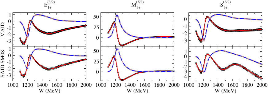
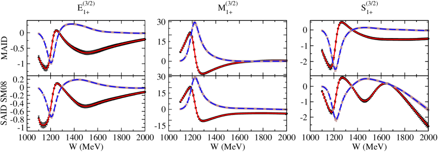
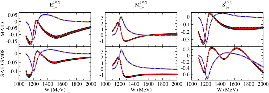
Figure 1: Figures showing the quality of the fit. We show all three multipoles at three intermediate momentum transfers $Q^{2}=0$, 1, and 5 GeV² for MAID2007 and SAID SM08 models. Black circles and brown squares are real and imaginary part of multipoles respectively. Full red line is real part and blue dashed line is imaginary part of the L+P fit to the given model.

V Results and Conclusions

In the L+P analysis, the pion electroproduction multipoles $E_{1+}^{(3/2)}(W,Q^{2})$, $M_{1+}^{(3/2)}(W,Q^{2})$, and $S_{1+}^{(3/2)}(W,Q^{2})$, from MAID2007 and SAID SM08, were fitted from threshold up to 2 GeV in the center-of-mass energy. These multipoles, which are accessible via the MAID and SAID web pages web , are displayed in Fig. 1.
For $Q^{2}$ values near the real-photon point, we fitted amplitudes from $Q^{2}=0$ to 0.5 GeV² in increments of 0.1 GeV². We then examined $Q^{2}$ values in increments of 1 GeV² up to 5 GeV², finding this region to have a less rapid variation. At each value of $Q^{2}$, amplitudes were analyzed in steps of 10 MeV.

Representative fit results covering the $\Delta(1232)$ energy range in Fig. 1 illustrate the very good fit quality and also display the rapid fall off of these amplitudes with $Q^{2}$. Numerical results from the $Q^{2}=0$ analyses are compiled in Table I.

In Fig. 2, we plot the associated helicity transition form factors, $A_{1/2}$, $A_{3/2}$, and $S_{1/2}$ as functions of $Q^{2}$. The $A_{1/2}$ and $A_{3/2}$ amplitudes, being dominated by the well-determined magnetic multipole, are very similar for the MAID and SAID analyses. The $S_{1/2}$ variation in $Q^{2}$ is qualitatively similar but differs in detail. It is interesting to note that, for the $A_{1/2}$ and $A_{3/2}$ amplitudes, the BW values and real parts of the pole quantities are nearly identical, particularly with increasing $Q^{2}$.

In Fig. 3, we compare the quantities $G_{M}/G_{D}$, and the $E/M$ and $S/M$ ratios as functions of $Q^{2}$, where $G_{D}=(1+Q^{2}/b^{2})^{-2}$, with $b^{2}$ = 0.71 (GeV/c)². Here also, the MAID and SAID results for $G_{M}/G_{D}$ agree very closely, with only a small difference between the BW values and real parts of the pole quantities. This pole behavior has also been displayed, over a smaller $Q^{2}$ range, in the analysis of Ref. suzu10 . The MAID and SAID BW results also agree well with the available single-$Q^{2}$ analyses of the $E/M$ ratio. These plots give no indication of a cross-over to positive $E/M$ values, as expected from Ref. carlson . Previously, both the MAID (2003) maid2003 and SAID (2002) vpi2002 fits had found indications for a cross over. This trend has disappeared with the incorporation of new and more precise measurements. The $S/M$ ratios of the MAID and SAID analyses display the only qualitative difference in $Q^{2}$ variation. Here also the BW and real part of the pole behavior is similar, with the SAID (pole and BW) curves tending to approximately follow the behavior of the single-$Q^{2}$ fits, whereas the MAID trend is for a slower $Q^{2}$ variation. We note that in the 2003 MAID analysis maid2003 , the $S/M$ ratio was found to have a more rapid $Q^{2}$ variation, following the trend of existing single-$Q^{2}$ values.

For low values of $Q^{2}$, we can also compare to the expectations from chiral effective theory Gail . In Fig. 4, the MAID and SAID quantities from Fig. 3 are compared to the predictions of Gail and Hemmert, Ref. Gail over a restricted $Q^{2}$ range. The range of applicability of their approach was estimated to about $Q^{2}_{max}\approx 0.2$ GeV². Due to the lack of data at the pole position, single-Q² data extracted at the BW position were used to determine the parameters of their approach. The result is a qualitatively good agreement between the real parts of pole-valued quantities, especially for the dominant magnetic transition, where even the imaginary part is reasonably described. However, this is not the case for $G_{E}$ and $G_{C}$. The real parts of these transitions are still in a moderate agreement, but the imaginary parts are off even by a different sign. This is not too surprising because the imaginary parts strongly depend on the parameters used for the pion loop integrals. A revised relativistic ChPT calculation in the complex mass scheme scherer2016 is in progress and may shed light on this issue.

	MAID Values			SAID Values
	BW	pole		BW	pole
$G_{M}$	$2.97$	$3.20$	$-4.7^{\circ}$	$3.11$	$3.38$	$-3.5^{\circ}$
$G_{E}$	$0.064$	$0.202$	$49^{\circ}$	$0.051$	$0.181$	$54^{\circ}$
$G_{C}$	$1.18$	$2.11$	$35^{\circ}$	$1.30$	$2.31$	$34^{\circ}$
$R_{EM}$	$-0.022$	$-0.063$	$53^{\circ}$	$-0.016$	$-0.054$	$58^{\circ}$
$R_{SM}$	$-0.042$	$-0.067$	$33^{\circ}$	$-0.044$	$-0.069$	$30^{\circ}$
$A_{1/2}$	$-0.131$	$-0.131$	$-20^{\circ}$	$-0.139$	$-0.142$	$-18^{\circ}$
$A_{3/2}$	$-0.247$	$-0.261$	$-7.7^{\circ}$	$-0.258$	$-0.273$	$-6.8^{\circ}$
$S_{1/2}$	$0.016$	$0.027$	$22^{\circ}$	$0.018$	$0.030$	$21^{\circ}$

Table 1: Magnetic, electric and charge transition form factors, $E/M$, $S/M$ ratios and photon decay amplitudes at $Q^{2}=0$ for the Breit-Wigner and for the pole position compared between MAID and SAID solutions. The BW parameters used for the conversion factor are: $M_{\Delta}=1232$  MeV and $\Gamma_{\pi}=\Gamma_{r}=115$ MeV, and the pole parameters are: $W_{p}=(1210-50i)$ MeV and $Res_{\pi N}=50\,e^{-i47^{\circ}}$. The form factors and ratios are dimensionless and the photon decay amplitudes are given in units of $10^{-3}/GeV^{1/2}$. For the complex values at the pole position, we give absolute values with the same sign as for the BW values and a phase.

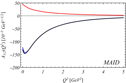
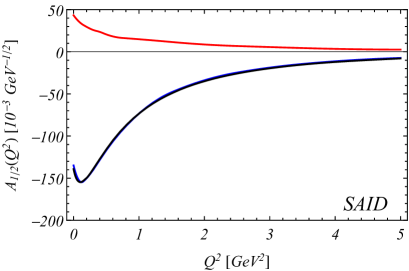
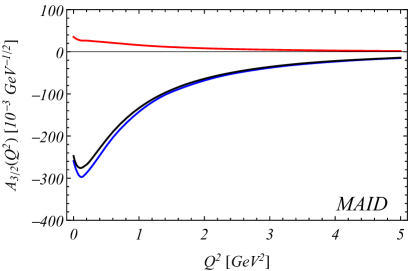
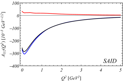
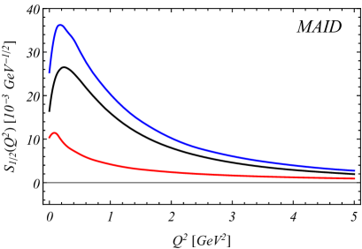
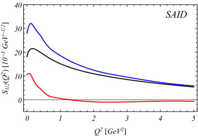
Figure 2: Helicity transition form factors $A_{1/2}$, $A_{3/2}$ and $S_{1/2}$ compared at the BW and pole position. The black curves show the real BW results and the blue and red lines show real and imaginary parts of the complex pole form factors. The left column shows the results with the Mainz-MAID analysis and the right column with the GWU-SAID analysis.

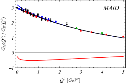
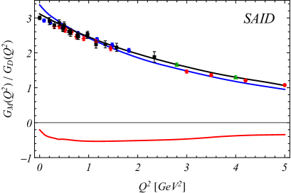
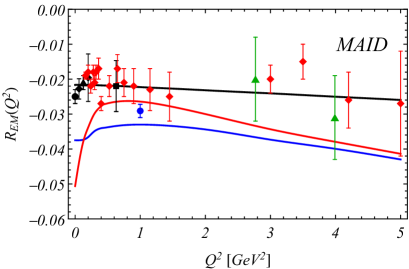
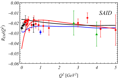
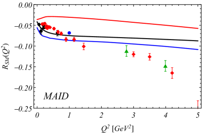
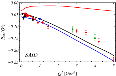
Figure 3: Magnetic transition form factor in the notation of Ash divided by the dipole form factor $G_{M}/G_{D}$ and $E/M$ and $S/M$ ratios compared at the BW and pole position. The black curves show the real BW results and the blue and red lines show real and imaginary parts of the complex pole form factors. The left column shows the results with the Mainz-MAID analysis and the right column with the GWU-SAID analysis. The data points for $G_{M}$ are from Refs: Beck00 (black circle), Bartel (black squares), Stein (blue circles), Fro99 (green triangles) and Azn09 (red diamonds); for $E/M$: Beck00 (black circle), Stave:2008tv (black diamonds), Mer01 (black triangle), Got00 ; Ban03 (black square), Kelly05 (blue circle), Fro99 (green triangles) and Azn09 (red diamonds); and for $S/M$: Stave:2008tv (black diamonds), Pos01 (black circle), Elsner06 (black triangle), Got00 ; Ban03 (black square), Kelly05 (blue circle), Fro99 (green triangles) and Azn09 (red diamonds).

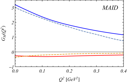
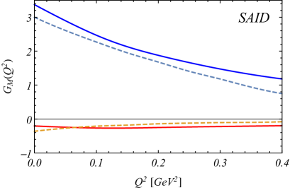
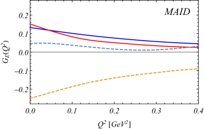
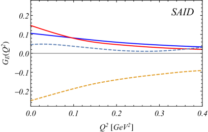
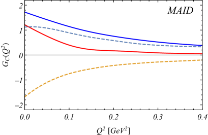
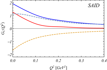
Figure 4: Magnetic, electric and charge transition form factors compared with the Heavy Baryon chiral effective field theory of Gail and Hemmert Gail at low $Q^{2}$. The blue and red lines show real and imaginary parts of the complex pole form factors obtained from MAID and SAID. The dashed lines are the HBChEFT calculations.

- (1) R. L. Workman, L. Tiator and A. Sarantsev, Phys. Rev. C 87, no. 6, 068201 (2013).
- (2) K. A. Olive et al. [Particle Data Group Collaboration], Chin. Phys. C 38, 090001 (2014); J. Beringer et al., Phys. Rev. D 86, 010001 (2012).
- (3) A.V. Anisovich, R. Beck, E. Klempt, V.A. Nikonov, A.V. Sarantsev, U. Thoma, Eur. Phys. J. A48, 15 (2012).
- (4) M. Döring, C. Hanhart, F. Huang, S. Krewald and U.-G. Meißner, Nucl. Phys. A 829, 170 (2009).
- (5) S. Ceci, M. Döring, C. Hanhart, S. Krewald, U.-G.Meissner, A. Svarc, Phys. Rev. C 84, 015205 (2011);
- (6) P. Masjuan, AIP Conf. Proc. 1343, 334 (2011);
- (7) S.N. Yang, Chin. J. Phys. 49, 1157 (2011);
- (8) L. Tiator, S.S. Kamalov, S. Ceci, G.Y. Chen, D. Drechsel, A. Svarc, S.N. Yang, Phys. Rev. C 82, 055203 (2010);
- (9) N. Suzuki, T. Sato, T.-S. H. Lee, Phys. Rev. C 82, 045206 (2010);
- (10) A. Svarc, M. Hadzimehmedovic, H. Osmanovic, J. Stahov, arXiv:1212.1295[nucl-th].
- (11) H. Kamano, S. X. Nakamura, T.-S. H. Lee and T. Sato, Phys. Rev. C 88, no. 3, 035209 (2013).
- (12) D. Rönchen, M. Döring, H. Haberzettl, J. Haidenbauer, U.-G. Meißner and K. Nakayama, Eur. Phys. J. A 51, 70 (2015).
- (13) D. Rönchen et al., Eur. Phys. J. A 50, 101 (2014) Erratum: [Eur. Phys. J. A 51, 63 (2015)].
- (14) T.A. Gail and T.R. Hemmert, Eur. Phys. J. A 28, 91 (2006).
- (15) V. Pascalutsa and M. Vanderhaeghen, Phys. Rev. D 73, 034003 (2006).
- (16) V. Bernard, T. R. Hemmert and U. G. Meißner, Phys. Lett. B 622, 141 (2005).
- (17) D. Jido, M. Döring and E. Oset, Phys. Rev. C 77, 065207 (2008).
- (18) M. Döring, Nucl. Phys. A 786, 164 (2007).
- (19) M. Döring, D. Jido and E. Oset, Eur. Phys. J. A 45, 319 (2010)
- (20) I. G. Aznauryan and V. D. Burkert, arXiv:1603.06692 [hep-ph].
- (21) G. Ramalho, M. T. Peña, J. Weil, H. van Hees and U. Mosel, Phys. Rev. D 93, 033004 (2016).
- (22) I. Aznauryan and V.D. Burkert, Phys. Rev. C 92, 035211 (2015).
- (23) J. Segovia, I.C. Cloët, C.D. Roberts, S.M. Schmidt, Few Body Syst. 55, 1185 (2014).
- (24) J. Segovia, C. Chen, I.C. Cloët, C.D. Roberts, S. M. Schmidt and S. Wan, Few Body Syst. 55, 1 (2014).
- (25) M. Ronniger and B. C. Metsch, Eur. Phys. J. A 49, 8 (2013).
- (26) H. Sanchis-Alepuz, R. Williams and R. Alkofer, Phys. Rev. D 87, no. 9, 096015 (2013).
- (27) G. Ramalho and M. T. Peña, Phys. Rev. D 85, 113014 (2012).
- (28) E. Santopinto and M. M. Giannini, Phys. Rev. C 86, 065202 (2012).
- (29) I. G. Aznauryan and V. D. Burkert, Prog. Part. Nucl. Phys. 67, 1 (2012).
- (30) E. Santopinto, A. Vassallo, M. M. Giannini and M. De Sanctis, Phys. Rev. C 82, 065204 (2010).
- (31) B. Juliá-Díaz et al., Phys. Rev. C 80, 025207 (2009).
- (32) M. Ungaro et al., Phys. Rev. Lett. 97, 112003 (2006).
- (33) M. Fiolhais, B. Golli and S. Sirca, Phys. Lett. B 373, 229 (1996).
- (34) V. Pascalutsa, M. Vanderhaeghen and S. N. Yang, Phys. Rept. 437, 125 (2007).
- (35) C. Alexandrou, J. W. Negele, M. Petschlies, A. Strelchenko and A. Tsapalis, Phys. Rev. D 88, no. 3, 031501 (2013)
- (36) C. Alexandrou, G. Koutsou, J. W. Negele, Y. Proestos and A. Tsapalis, Phys. Rev. D 83, 014501 (2011)
- (37) A. Agadjanov, V. Bernard, U.-G. Meißner and A. Rusetsky, Nucl. Phys. B 886, 1199 (2014)
- (38) A. Švarc, M. Hadžimehmedović, H. Osmanović, J. Stahov, L. Tiator, and R. L. Workman, Phys. Rev. C88, 035206 (2013).
- (39) A. Švarc, M. Hadžimehmedović, R. Omerović, H. Osmanović, and J. Stahov, Phys. Rev. C89, 45205 (2014).
- (40) A. Švarc, M. Hadžimehmedović, H. Osmanović, J. Stahov, and R. L. Workman, Phys. Rev. C91, 015207 (2015).
- (41) A. Švarc, M. Hadžimehmedović, H. Osmanović, J. Stahov, L. Tiator, and R. L. Workman, Phys. Rev. C89, 065208 (2014).
- (42) A. Švarc, M. Hadžimehmedović, H. Osmanović, J. Stahov, L. Tiator, and R. L. Workman, Phys. Lett. B755, 452-455 (2016).
- (43) C. Becchi and G. Morpurgo, Phys. Lett. 17, 352 (1965).
- (44) C.E. Carlson, Phys. Rev. D 34, 2704 (1986).
- (45) W. W. Ash et al., Phys. Lett. B 24 (1967) 165.
- (46) H. F. Jones and M. D. Scadron, Annals Phys. 81, 1 (1973).
- (47) L. Tiator, D. Drechsel, S. S. Kamalov and M. Vanderhaeghen, Eur. Phys. J. ST 198, 141 (2011).
- (48) R. C. E. Devenish, T. S. Eisenschitz, J. G. Körner, Phys. Rev. D14 (1976) 3063.
- (49) D. Drechsel, S.S. Kamalov, L. Tiator, Nucl. Phys. A34, 69 (2007).
- (50) M. Döring, C. Hanhart, F. Huang, S. Krewald and U.-G. Meißner, Phys. Lett. B 681, 26 (2009).
- (51) G. Höhler, N Newsletter 9, 1 (1993).
- (52) R. E. Cutkosky, C. P. Forsyth, R. E. Hendrick, and R.L. Kelly, Phys. Rev. D 20, 2839 (1979).
- (53) S. Ceci, J. Stahov, A. Švarc, S. Watson, and B. Zauner, Phys. Rev. D 77, 116007 (2008).
- (54) Amplitudes are available from the MAID site: http://portal.kph.uni-mainz.de/MAID// and from the SAID site: http://gwdac.phys.gwu.edu.
- (55) L. Tiator, D. Drechsel, S.S. Kamalov, S.N. Yang, Eur. Phys. J. A 17, 357 (2003).
- (56) R.A. Arndt, W. Briscoe, I. Strakovsky, R. Workman, p.234, proceedings of the Workshop on the Physics of Excited Nucleons (NSTAR2002), Pittsburgh, PA, 2002. Ed. S.A. Dytman and E.S. Swanson (World Scientific, 2003).
- (57) M. Hilt, T. Bauer, S. Scherer, L. Tiator, in preparation.
- (58) S. Stave et al. [ A1 Collaboration ], Phys. Rev. C78 (2008) 025209.
- (59) I. G. Aznauryan et al. [ CLAS Collaboration ], Phys. Rev. C80 (2009) 055203.
- (60) W. Bartel et al., Phys. Lett. 28B (1968) 148
- (61) S. Stein et al., Phys. Rev. D12 (1975) 1884.
- (62) Th. Pospischil et al., Phys. Rev. Lett. 86 (2001) 2959.
- (63) D. Elsner et al., Eur. Phys. J. A 27 (2006) 91.
- (64) S. Stave et al., Eur. Phys. J. A 30 (2006) 471.
- (65) R. W. Gothe, Prog. Part. Nucl. Phys. 44 (2000) 185.
- (66) T. Bantes, PhD thesis, Bonn 2003.
- (67) C. Mertz et al., Phys. Rev. Lett. 86 (2001) 2963.
- (68) R. Beck et al., Phys. Rev. C 61 (2000) 035204.
- (69) J. J. Kelly et al., Phys. Rev. Lett. 95 (2005) 102001 and Phys. Rev. C 75 (2007), 025201.
- (70) V. V. Frolov et al., Phys. Rev. Lett. 82 (1999) 45.