Monte Carlo analysis for finite temperature magnetism of Nd₂Fe₁₄B permanent magnet

Abstract

We investigate the effects of magnetic inhomogeneities and thermal fluctuations on the magnetic properties of a rare earth intermetallic compound, Nd₂Fe₁₄B. The constrained Monte Carlo method is applied to a Nd₂Fe₁₄B bulk system to realize the experimentally observed spin reorientation and magnetic anisotropy constants $K^{\rm A}_{m}(m=1,2,4)$ at finite temperatures. Subsequently, it is found that the temperature dependence of $K^{\rm A}_{1}$ deviates from the Callen–Callen law, $K^{\rm A}_{1}(T)\propto M(T)^{3}$, even above room temperature, $T_{\rm R}\sim 300\rm\,K$, when the Fe (Nd) anisotropy terms are removed to leave only the Nd (Fe) anisotropy terms. This is because the exchange couplings between Nd moments and Fe spins are much smaller than those between Fe spins. It is also found that the exponent $n$ in the external magnetic field $H_{\rm ext}$ response of barrier height $\mathcal{F}_{\rm B}=\mathcal{F}_{\rm B}^{0}(1-H_{\rm ext}/H_{0})^{n}$ is less than $2$ in the low-temperature region below $T_{\rm R}$, whereas $n$ approaches $2$ when $T>T_{\rm R}$, indicating the presence of Stoner–Wohlfarth-type magnetization rotation. This reflects the fact that the magnetic anisotropy is mainly governed by the $K^{\rm A}_{1}$ term in the $T>T_{\rm R}$ region.

I Introduction

Rare earth permanent magnets, particularly Nd-Fe-B, exhibiting strong magnetic performanceHerbst (1991) are attracting considerable attention because of the rapidly growing interest in electric vehicles. The main focus of research in involving these materials is to increase the coercive field $H_{c}$ and improve the temperature dependence.Fidler and Knoch (1989); Vial et al. (2002); Li et al. (2009); Woodcock et al. (2012); Hono and Sepehri-Amin (2012) Therefore, a number of studies have conducted micromagnetic simulations Kronmüller et al. (1987); Sakuma et al. (1990); Fischer et al. (1996); Hrkac et al. (2010) for the magnetization processes using inhomogeneous magnetic parameters to describe the complex structures in sintered magnets. Many of the results predict that the distinctive feature of magnetic anisotropy near the grain boundaries of Nd-Fe-B particles is responsible for the degradation of $H_{c}$.

Thus, one of the remaining subjects of the theoretical study is to give quantitative aspects in microscopic viewpoint or in atomic-scale, to the $m$-th order magnetic anisotropy constants $K^{\rm A}_{m}$ and their temperature dependence near the grain surfaces or grain boundaries. For $K^{\rm A}_{1}$ at the surface of Nd-Fe-B particles, Moriya et al. Moriya et al. (2009) and Tanaka et al. Tanaka et al. (2011) calculated the crystal field parameter $A_{2}^{0}$ using a first-principles technique and pointed out that $K^{\rm A}_{1}$ (mainly proportional to $A_{2}^{0}$) is negative at the $(001)$ surface when the $(001)$ Nd layer is exposed to a vacuum. However, few theoretical studies have examined the temperature dependence of $K^{\rm A}_{m}$, even for the bulk system, since the qualitative theory was developed by Callen and Callen.Callen and Callen (1963, 1966); Skomski and Coey (1999)Recently, Sasaki et al. Sasaki et al. (2015) and Miura et al. Miura et al. (2015) conducted theoretical studies in the quantitative level on the temperature dependence of $K^{\rm A}_{m}$ for a Nd₂Fe₁₄B bulk system based on crystal field theory, and successfully reproduced various experimental results. However, as these theories relied on the mean field approach in terms of the exchange coupling between the Nd $4f$ moments and Fe $3d$ spins, the results cannot be directly applied to $K^{\rm A}_{m}$ near the surfaces or interfaces of particles. Moreover, because the crystal field analysis employed in these works is based on a quantum mechanical approach, which is typical for $4f$ electronic systems,Yamada et al. (1988) it is effectively impossible to treat finite systems of nm- or $\mu$m-scale using a similar method.

Therefore, in the present work, in anticipation of future work on magnetization reversal in finite-sized particles, we employed a realistic model with a classical Heisenberg Hamiltonian to calculate the magnetic properties of a Nd₂Fe₁₄B bulk system at finite temperatures. The key features of our model are: 1) an appropriate crystalline electric field HamiltonianYamada et al. (1988) is included in the classical manner, 2) exchange coupling parameters are obtained by first-principles calculations, 3) $K^{\rm A}_{m}$ is directly evaluated from Monte Carlo (MC) simulations without employing the mean field analysis, and 4) the constrained Monte Carlo (C-MC) method,Asselin et al. (2010) is adopted to evaluate the temperature dependence of magnetic anisotropy. Note that we can naturally realize the experimentally observed spin reorientation and $K^{\rm A}_{m}$. Reflecting the (inhomogeneous) variation of magnetic parameters in the unit cell composed of $68$ atoms (see Fig. 1), $K^{\rm A}_{1}$ does not obey the Callen–Callen law,Callen and Callen (1963, 1966) which states that $K^{\rm A}_{1}(T)\propto M(T)^{3}$ when considering only the Nd (Fe) anisotropy terms and neglecting the Fe (Nd) anisotropy terms. We also analyze the response of the external magnetic field $H_{\rm ext}$Gaunt (1986); Chantrell et al. (2000); Suess et al. (2007); Bance et al. (2015a, b); Goto et al. (2015) for a barrier height $\mathcal{F}_{\rm B}(H_{\rm ext})=\mathcal{F}_{\rm B}^{0}(1-H_{\rm ext}/H_{0})^{n}$, and find that the $H_{\rm ext}$ response deviates from the Stoner–Wohlfarth-type ($n=2$), especially below room temperature, $T_{\rm R}\sim 300\,\rm K$.

II Model and Method

II.1 Model

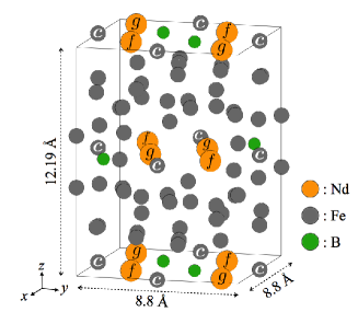
Figure 1: Unit cell of Nd₂Fe₁₄B including $68$ atoms (space group:$P4_{2}/mnm$ (No.136)). Herbst et al. (1984) Only Nd($f,g$) and Fe$(c)$ sites are represented. This figure was plotted using VESTA.Momma and Izumi (2011)

By treating each atom as having classical spin, we constructed a three-dimensional Heisenberg model including realistic atom locations for Nd₂Fe₁₄B, as shown in Fig. 1. This model using atomic-scale parameters was defined as follow:

$${\cal H} = -2\sum_{i<j}S_{i}J^{\rm ex}_{ij}S_{j}{\bm{e}}_{i}\cdot{\bm{e}}_{j}-\mu_{0}\sum_{i}m_{i}\bm{e}_{i}\cdot\bm{H}_{\rm ext}$$

$$-\sum_{i\in{\rm TM}}D_{i}^{\rm A}(e^{z}_{i})^{2}+\sum_{i\in{\rm RE}}\sum_{l=2,4,6}\tilde{\theta}_{l}^{{J}_{i}}A_{l,i}^{m_{l}}\langle r^{l}\rangle_{i}\hat{\mathcal{O}}^{m_{l}}_{l,i},$$

where $S_{i}J^{\rm ex}_{ij}S_{j}$ is the exchange coupling constant including the spin amplitude between the $i$-th and $j$-th sites, ${\bm{e}}_{i}$ is the normalized spin vector at the $i$-th site, $m_{i}$ is the magnetic moment, $\mu_{0}$ is the magnetic permeability of a vacuum and $\bm{H}_{\rm ext}$ is the external magnetic field. The third and fourth terms include single-ion magnetic anisotropy properties. We consider transition metals (TM) and rare-earth elements (RE) separately. The anisotropy of TM sites is defined using the magnetic anisotropy parameter $D^{\rm A}_{i}$ and the $z$-component of $\bm{e}_{i}$, i.e., $e^{z}_{i}$. The anisotropy of RE sites is based on crystal field theoryStevens (1952); Yamada et al. (1988) and uses the Stevens operator $\hat{\mathcal{O}}_{l,i}^{m_{l}}$, crystal field parameter $A_{l,i}^{m_{l}}$, and Stevens factor $\tilde{\theta}_{l}^{{J}_{i}}$. Here, $\langle r^{l}\rangle_{i}$ can be calculated as the spatial average of the $4f$ electron distribution. In the present paper, we consider $m_{l}=0$ for simplicity. For reference, note that $\hat{\mathcal{O}}_{l,i}^{m_{l}=0}$ and $\tilde{\theta}_{l}^{J=\frac{9}{2}}$:

$$\hat{\mathcal{O}}_{2,i}^{0} = 3(J^{z}_{i})^{2}-J_{i}^{2},$$

$$\hat{\mathcal{O}}_{4,i}^{0} = 35(J^{z}_{i})^{4}-\bigl{[}30{J}_{i}^{2}-25\bigr{]}(J^{z}_{i})^{2}+\bigl{[}3{J}_{i}^{4}-6{J}_{i}^{2}\bigr{]},$$

$$\hat{\mathcal{O}}_{6,i}^{0} = 231(J^{z}_{i})^{6}-\bigl{[}315{J}_{i}^{2}-735\bigr{]}(J^{z}_{i})^{4}$$ (2)

$$\quad\qquad+\bigl{[}105{J}_{i}^{4}-525{J}_{i}^{2}+294\bigr{]}(J^{z}_{i})^{2}$$

$$\quad\qquad-\bigl{[}5{J}_{i}^{6}-40{J}_{i}^{4}+60{J}_{i}^{2}\bigr{]},$$

$$\tilde{\theta}_{2}^{\rm\frac{9}{2}}=\frac{-7}{3^{2}\cdot 11^{2}},\ \tilde{\theta}_{4}^{\rm\frac{9}{2}}=\frac{-2^{3}\cdot 17}{3^{3}\cdot 11^{3}\cdot 13},\ \tilde{\theta}_{6}^{\rm\frac{9}{2}}=\frac{-5\cdot 17\cdot 19}{3^{3}\cdot 7\cdot 11^{3}\cdot 13^{2}},$$

where $J^{z}_{i}={J}_{i}{e}^{z}_{i}$ is the $z$-component of the total angular momentum ${J}_{i}$, which is $9/2$ for Nd atoms, and we use $J_{i}^{2}$ instead of $J_{i}(J_{i}+1)$ in the classical manner.

Table 1: Site occupancies and model parameters of each crystallographically inequivalent atom. The spin magnetic moments, $m^{s}$, are calculated from the first-principles calculation code, Machikaneyama (AkaiKKR).aka The anisotropy parameters $D^{\rm A}_{i_{\rm TM}}$ and $A_{l}^{{\color[rgb]{0,0,0}m_{l}}}\langle r^{l}\rangle$ are taken from previous results.Miura et al. (2014); Yamada et al. (1988) We neglected the $D^{\rm A}$ values of B and Nd, as they are less than $0.1\,\rm meV$, and used the $\langle r^{l}\rangle$ values of Nd, Ref. 31, i.e., $\langle r^{2}\rangle=1.001\,{\color[rgb]{0,0,0}a_{B}^{2}}$, $\langle r^{4}\rangle=2.401\,{\color[rgb]{0,0,0}a_{B}^{4}}$, and $\langle r^{6}\rangle=12.396\,{\color[rgb]{0,0,0}a_{B}^{6}}$, where $a_{B}$ is the Bohr radius.

atom	occ.	$m^{s}$ [$\mu_{B}$]	$D^{\rm A}_{i_{\rm TM}}$ [meV]	$A_{l}^{{\color[rgb]{0,0,0}m_{l}}}\langle r^{l}\rangle$ [K]
B($g$)	4	-0.169	-	-
Fe($c$)	4	2.531	-2.14	-
Fe($e$)	4	1.874	-0.03	-
Fe($j_{1}$)	8	2.298	1.07	-
Fe($j_{2}$)	8	2.629	0.58	-
Fe($k_{1}$)	16	2.063	0.55	-
Fe($k_{2}$)	16	2.206	0.38	-
			($l,{\color[rgb]{0,0,0}m_{l}}$):	($2,0$)	($4,0$)	($6,0$)
Nd($f$)	4	-0.413	-	295.3	-29.5	-22.8
Nd($g$)	4	-0.402	-

Table 1 lists the atomic-scale parameters used in the present study. The $68$ atoms in the tetragonal unit cell of Nd₂Fe₁₄B (see Fig. 1) occupy nine crystallographically inequivalent sites, as seen in Table 1. These atom locations and lattice constants ($a=b=8.8$ Å, $c=12.19$ Å) were set to experimental values.Herbst et al. (1984) $m^{s}$ is the spin magnetic moment of valence electrons (excluding $4f$-electrons). We defined $m_{i}=m^{s}_{i}$ for Fe and B atoms, and $m_{i}=m^{s}_{i}+m^{4f}_{i}$ for Nd atoms. Here, the magnetic moment of $4f$-electrons in each Nd atom is $m^{4f}=8J/11\,\mu_{B}\sim 3.273\,\mu_{B}$. For the magnetic anisotropy terms, the $D^{\rm A}$ values were set to previous first-principles calculation resultsMiura et al. (2014) for Y₂Fe₁₄B, which has a similar crystal structure as Nd₂Fe₁₄B. In contrast, we adopted experimental resultsYamada et al. (1988) regarding $A_{l}^{{\color[rgb]{0,0,0}m_{l}}}$, even though some research for the $A_{l}^{{\color[rgb]{0,0,0}m_{l}}}$ values of Nd₂Fe₁₄B was performed using first-principles calculations.Hummler and Fähnle (1996); Yoshioka et al. (2015) This is because first-principles evaluations of $A_{l}^{{\color[rgb]{0,0,0}m_{l}}}$ are strongly dependent on the calculation conditions; in particular, the values of the $l=6$ terms are still open to some debate.

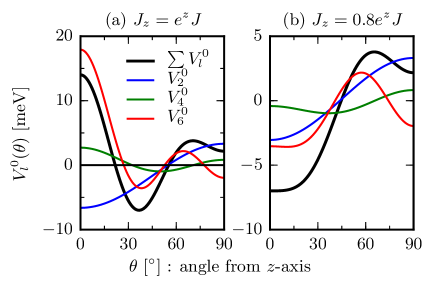
Figure 2: Anisotropy potentials $V_{l}^{0}(\theta)\,{\color[rgb]{0,0,0}\rm[meV]}$ for $J=9/2$ single spin. Black lines denote total anisotropy potential $V_{2}^{0}+V_{4}^{0}+V_{6}^{0}$.

The higher-order crystal field parameters $A_{4}^{0}$ and $A_{6}^{0}$ of the Nd atoms have a significant effect on the low-temperature properties of Nd₂Fe₁₄B. To illustrate these effects, Fig. 2 shows the anisotropy potential for $J=9/2$ single classical spin:

$$V_{l}^{m_{l}}(\theta)=\tilde{\theta}_{l}^{\frac{9}{2}}A_{l}^{m_{l}}\langle r^{l}\rangle\hat{\mathcal{O}}^{m_{l}}_{l}(\theta),$$ (3)

where $\theta$ is the spin angle measured from the $z$-axis (i.e., $e^{z}=\cos\theta$) and $A_{l}^{m_{l}}\langle r^{l}\rangle$ take the values in Table 1. The potential $V_{2}^{0}$ increases monotonically as $\theta$ increases, whereas $V_{4}^{0}$ and $V_{6}^{0}$ vary non-monotonically. Because of this behavior, the total anisotropy potential $V_{2}^{0}+V_{4}^{0}+V_{6}^{0}$ attains a minimum at $\theta=36.7^{\circ}$ for (a) $J_{z}=e^{z}J$. In contrast, for (b) $J_{z}=0.8e^{z}J$, the minimum occurs at $\theta=0^{\circ}$. This coefficient ($=0.8$) of $e^{z}$ can be regarded as an effect of thermal fluctuations at $T>0$. The above results indicate that the spin direction is tilted from the $z$-axis at $T=0$, although this tilting disappears at a certain temperature. This behavior corresponds to the spin reorientation phenomenon. In the case of Nd₂Fe₁₄B, the spin reorientation transition is due to the $V_{4}^{0}$ and $V_{6}^{0}$ values of Nd atoms, and includes the effects of exchange couplings and the magnetic anisotropy of Fe atoms (for details, see Sec. III.1).

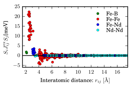
Figure 3: Exchange coupling constant between each atom as a function of interatomic distance.

Figure 3 shows the exchange coupling constants, $S_{i}J^{\rm ex}_{ij}S_{j}$, which include the spin amplitude as a function of interatomic distance $r_{ij}$. These constants were calculated with Liechtenstein’s formula Liechtenstein et al. (1987) that has been implemented on the first-principles electronic-structure calculation using the Korringa-Kohn-Rostoker (KKR) Green’s function method, Machikaneyama (AkaiKKR).aka In the calculation, standard muffin-tin-type potentials were assumed, and the local density approximation parametrized by Morruzi, Janak and Williams Moruzzi et al. (1978) was used. Up to $d$-wave scatterings were taken into account in KKR, and ($8\times 8\times 6$) $k$-points in the first Brillouin zone being used for the calculation of $J^{\rm ex}_{ij}$’s. For the Nd 4f-states, the so called open-core approximation was employed.

From Fig. 3, we can see that the exchange couplings between Fe and Nd have much smaller values than those between Fe atoms. In addition, none of the Nd atoms interacts directly with other Nd atoms. The amplitude relation of the exchange couplings is consistent with experimental resultsHerbst (1991) based on a mean field analysis. Note that all $S_{\rm Fe}J_{\rm Fe\mathchar 28973\relax Nd}^{\rm ex}S_{\rm Nd}$ on $r_{ij}<4$ Å have positive values in Fig. 3. As $J_{ij}^{\rm ex}$ is evaluated as the interaction between valence electrons, $S_{\rm Fe(Nd)}$ can be regarded as being proportional to $m^{s}_{\rm{Fe(Nd)}}$, i.e., $S_{\rm Nd}S_{\rm Fe}<0$. Hence, the bare exchange couplings $J_{\rm Fe\mathchar 28973\relax Nd}^{\rm ex}$ have negative values. The couplings between Fe and B, $J_{\rm Fe\mathchar 28973\relax B}^{\rm ex}$, also take negative values which can be explained in the same way.

II.2 Method

To analyze the finite-temperature magnetism of Nd₂Fe₁₄B, we applied MC methods based on the Metropolis algorithmLandau and Binder (2014) to the above classical Heisenberg model. Although the magnetic anisotropy is evaluated as the magnetization angle dependence of free energy, this is generally difficult to simulate explicitly using a typical MC approach. Therefore, we also adopted the C-MC methodAsselin et al. (2010) to evaluate the magnetic anisotropy. The C-MC method fixes the direction of total magnetization $\bm{M}=(M_{x},M_{y},M_{z})=(1/N_{s})\sum_{i}m_{i}\bm{e}_{i}$ ($N_{s}$ is the total number of sites) in any direction for each MC sampling without $\bm{H}_{\rm ext}$, and then calculates the fixed angle $\theta$ dependencies of free energy $\Delta\mathcal{F}(\theta)$ and magnetization torque $\vec{\mathcal{T}}(\theta)$ as follows:Asselin et al. (2010)

$$\vec{\mathcal{T}}(\theta) = -\left\langle\sum_{i}{\bm{e}}_{i}\times\frac{\partial\mathcal{H}}{\partial{\bm{e}}_{i}}\right\rangle\quad\text{for}\ \bm{M}=\bm{M}(\theta),$$ (4)

$$\Delta\mathcal{F}(\theta) = \mathcal{F}(\theta)-\mathcal{F}(\theta_{0})$$ (5)

$$= \int_{\theta_{0}}^{\theta}d\theta^{\prime}\,\left[{\color[rgb]{0,0,0}{\bm{n}}}(\theta^{\prime})\times\vec{\mathcal{T}}(\theta^{\prime})\right]\cdot\left.\frac{\partial{\color[rgb]{0,0,0}\bm{n}}(\theta)}{\partial\theta}\right|_{\theta=\theta^{\prime}},$$

where $\bm{n}(\theta)=\bm{M}(\theta)/|\bm{M}(\theta)|$ and $\bm{M}(\theta)$ is the total magnetization in the fixed direction $\theta$.

Note that Asselin et al.Asselin et al. (2010) formulated the C-MC method for systems with homogeneous magnetic moments, i.e. all the magnetic moments have same value. However, it can easily be extended to systems with inhomogeneous magnetic moments such as Nd₂Fe₁₄B. We now briefly explain only the procedure of the extended C-MC method with a fixed $M$ in the direction of $z$-axis:

• Select a site $i$ and obtain the new state of $i$-spin randomely chosen,

  $$\bm{e}_{i}\rightarrow\bm{e}^{\prime}_{i}.$$

• Select a site $j(\neq i)$ randomly.

• Adjust the new state of the $j$-spin to preserve $\bm{M}$ direction (namely, $M_{x}=M_{y}=0$):

  $$\bm{e}_{j} \rightarrow \bm{e}^{\prime}_{j},$$

  $$e^{x\prime}_{j} =e^{x}_{j}+\frac{m_{i}}{m_{j}}(e^{x}_{i}-e^{x\prime}_{i}),$$

  $$e^{y\prime}_{j} =e^{y}_{j}+\frac{m_{i}}{m_{j}}(e^{y}_{i}-e^{y\prime}_{i}),$$

  $$e^{z\prime}_{j} ={\rm sign}(e^{z}_{j})\sqrt{1-(e^{x\prime}_{j})^{2}-(e^{y\prime}_{j})^{2}}.$$

  If $1-(e^{x\prime}_{j})^{2}-(e^{y\prime}_{j})^{2}<0$, return to (A).

• Calculate the new total magnetization:

  $$\bm{M}^{\prime} = \bm{M}+\frac{1}{N_{s}}\left[m_{i}(\bm{e}^{\prime}_{i}-\bm{e}_{i})+m_{j}(\bm{e}^{\prime}_{j}-\bm{e}_{j})\right].$$

  If $\bm{M}^{\prime}<0$, return to (A).

• Update from the initial spin states ($\bm{e}_{i},\bm{e}_{j}$) to the new spin states ($\bm{e}^{\prime}_{i},\bm{e}^{\prime}_{j}$) with the probability:

  $$P = {\rm min}\left[1,\left(\frac{M_{z}^{\prime}}{M_{z}}\right)^{2}\frac{|e_{j}^{z}|}{|e_{j}^{z\prime}|}\exp{(-\beta\Delta E)}\right],$$

  where $\beta$ is the inverse temperature and $\Delta E=E(\bm{e}^{\prime}_{i},\bm{e}^{\prime}_{j})-E(\bm{e}_{i},\bm{e}_{j})$ is the energy difference.

• Return to (A).

To apply C-MC method to the Nd₂Fe₁₄B bulk system, we change the procedures (C) and (D) to treat different magnetic moments from those in the original pepar.Asselin et al. (2010)

The MC (C-MC) simulations in the present study repeated each calculation for 200,000 (100,000) MC steps, where one MC step is defined as one trial for each spin to be updated. The first 100,000 (30,000) MC steps were used for equilibration, and the following 100,000 (70,000) MC steps were used to measure the physical quantities. We performed simulations for 12 different runs with different initial conditions and random sequences. We then calculated the average results and statistical errors. To check the system-size dependence, we used systems of $N_{s}$=$L^{3}\times$ $68$ (unit cell) sites with $L=3$–$6$, imposing the periodic boundary conditions.

III Results and Discussion

III.1 Thermodynamic Properties

First, we focus on the magnetic transition points to verify the model and parameter values. The results in this subsection are based on typical MC, rather than C-MC.

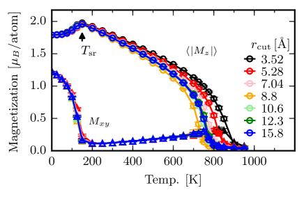
Figure 4: Magnetizations as a function of temperature for each effective exchange coupling radius $r_{\rm cut}$. System size is $L=6$.

Figure 4 shows the magnetization curves for each cutoff range $r_{\rm cut}$. We consider all exchange couplings $J_{ij}^{\rm ex}$ under $r_{ij}\leq r_{\rm cut}$. Here, $\langle A\rangle$ is defined as the statistical average of $A$. It can be seen that there are two transition points in Fig. 4.

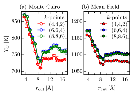
Figure 5: Curie temperatures with (a) MC and (b) mean field as a function of effective exchange coupling radius $r_{\rm cut}$ for the number of $k$-points.

In the higher-temperature region, $\langle|M_{z}|\rangle$ approaches $0$ at the Curie temperature $T_{\rm C}$. The magnetization curves show that $T_{\rm C}$ is strongly dependent on $r_{\rm cut}$, even in long-range ($r_{ij}>3.52\,{\rm\AA}$). Thus, $T_{\rm C}$ was evaluated more accurately using the Binder parameterBinder (1981a, b); Landau and Binder (2014) defined as $g_{L}=1-\langle|\bm{M}|\rangle^{4}/3\langle|\bm{M}|^{2}\rangle^{2}$, for system sizes $L=3$–$6$. The results are plotted in Fig. 5(a). It is apparent that $T_{\rm C}$ has quite different values depending on $r_{\rm cut}$, and the condition of $(8\times 8\times 6)$ $k$-points (mean accuracy of $S_{i}J_{ij}^{\rm ex}S_{j}$ in the first-principles calculations) is sufficient for convergence. Similar behavior can be seen in Fig. 5(b), where $T_{\rm C}$ has been calculated by a $9$-sublattice (i.e., $9$-inequivalent sites in Table 1) mean field analysis.Herbst and Croat (1984); Skomski (1998) Compared with the MC results, the mean field results are less sensitive to $r_{\rm cut}$ and tend to overestimate $T_{\rm C}$.

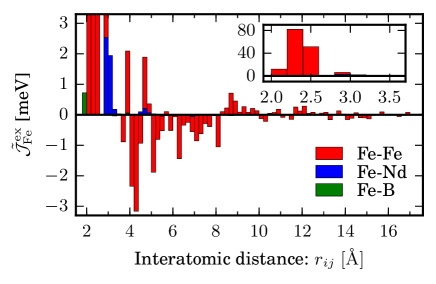
Figure 6: Average Fe atom exchange coupling $\tilde{\mathcal{J}}^{\rm ex}_{\rm Fe}$ as a function of $r_{ij}$. Inset shows a large-area view of $\tilde{\mathcal{J}}^{\rm ex}_{\rm Fe}$ in $r_{ij}<3.7\,\rm\AA$.

To analyze the long-range ($r_{ij}>3.52\,{\rm\AA}$) exchange coupling effect for $T_{\rm C}$, Fig. 6 shows the average exchange coupling at the Fe atoms, $\tilde{\mathcal{J}}^{\rm ex}_{\rm Fe}(r_{1},r_{2})$, which is defined as follows:

$$\tilde{\mathcal{J}}^{\rm ex}_{\rm Fe}(r_{1},r_{2})=\frac{1}{N_{\rm Fe}}\sum_{i\in{\rm Fe},j}S_{i}J^{\rm ex}_{ij}S_{j}\ {\rm for}\ r_{1}<r_{ij}\leq r_{2},$$ (6)

where $N_{\rm Fe}$ is the total number of Fe sites. Each bar height in Fig. 6 denotes the sum of $S_{i}J^{\rm ex}_{ij}S_{j}$ per atom in the range of each bar width (here $r_{2}-r_{1}=0.2\,{\rm\AA}$). Because $\tilde{\mathcal{J}}_{\rm Fe}^{\rm ex}$ has many exchange bonds that correspond to a spherical surface area ($\propto r_{ij}^{2}$), it keeps small but significant value even in the long range. Indeed, the sum of short-range exchange couplings is $\tilde{\mathcal{J}}^{\rm ex}_{\rm Fe}(0,3.52\,{\rm\AA})=154.6\,$meV and that over a longer range is $\tilde{\mathcal{J}}^{\rm ex}_{\rm Fe}(3.52\,{\rm\AA},17.6\,{\rm\AA})=-10.2$ meV. This negative value explains the decreasing trend for $T_{\rm C}$ shown in Fig. 5. The necessity of long-range exchange coupling has been identified for bcc-Fe Spišák and Hafner (1997); Singer et al. (2011); Kvashnin et al. (2016) and MnBi,Williams et al. (2016) and so the dependence of $r_{\rm cut}$ appears to reflect the features of itinerant ferromagnetism. Under the condition that $r_{\rm cut}=3.52$, $10.6$, and $17.6\,\rm\AA$, each atom has approximately 13, 350, and 1660 exchange coupling bonds, respectively. To reduce the computational load, we mainly consider $r_{\rm cut}=10.6\,\rm\AA$.

At the lower temperature point $T_{\rm sr}\,(\sim 145\,{\rm K})$ in Fig. 4, $\langle|M_{z}|\rangle$ reaches a maximum and ${\color[rgb]{0,0,0}M_{xy}=}\sqrt{\langle M_{x}^{2}\rangle+\langle M_{y}^{2}\rangle}$ approaches $0$, which is known to be the spin-reorientation transition of the Nd₂Fe₁₄B magnet. The magnetization direction is tilted $34.4^{\circ}$ from the $z$-axis at $T=0$ for every $r_{\rm cut}$. Above $T_{\rm sr}$, this direction exhibits uniaxial anisotropy along the $z$-axis. In contrast to $T_{\rm C}$, $T_{\rm sr}$ has only a weak dependence on $r_{\rm cut}$. The spin-reorientation transition is mainly driven by the higher-order terms ($l=4,6$) of $A_{l}^{{\color[rgb]{0,0,0}m_{l}=0}}$ on the Nd atoms in Eq. (LABEL:eq:hami). Indeed, in comparison to the tilting angle of the single Nd atom at $T=0$ ($\theta=36.7^{\circ}$ in Fig. 2(a)), we can see that the Fe magnetic anisotropy has little effect on the spin reorientation. The reorientation property of Nd atoms is shared with the whole Nd₂Fe₁₄B through the exchange coupling $J^{\rm ex}_{\rm Fe\mathchar 28973\relax Nd}$. As shown in Fig. 6, most contributions of $J^{\rm ex}_{\rm Fe\mathchar 28973\relax Nd}$ are in the range $r_{\rm cut}\leq 3.4$ Å. Therefore, $T_{\rm sr}$ has only a weak dependence on the long-range parts of $J^{\rm ex}_{ij}$.

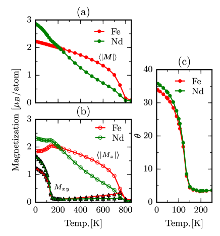
Figure 7: Temperature dependence of (a) the magnetization amplitude: $\langle|\bm{M}|\rangle$, (b) $z$-component: $\langle|M_{z}|\rangle$ and $xy$-component: $M_{xy}$ of Fe and Nd atoms for $r_{\rm cut}=10.6\,{\rm\AA}$ and $L=6$. (c) Each magnetization angle measured from $z$-axis at low-temperature region.

To look into the role for each atom in the above two transition at $T_{\rm C}$ and $T_{\rm sr}$, we plot in Fig. 7 the temperature dependence of the magnetizations and the magnetization angle of Nd and Fe atoms. In Fig. 7(a), reduction of the magnetization amplitude $\langle|M|\rangle$ with the temperature of each atom shows clear difference. This difference is reflected by the amplitude of exchange couplings, $\tilde{\mathcal{J}}^{\rm ex}_{\rm Fe}$ ($\tilde{\mathcal{J}}^{\rm ex}_{\rm Nd}$) for $r_{1}=0$, $r_{2}=10.6\rm\,\AA$ is $142.9\,\rm meV$ ($33.5\,\rm meV$). Hence, The ferromagnetic order of Fe is responsible to the magnetic order of the magnets. At high temperature, we may have a picture that the magnetization of Nd atom is maintained by the interaction with the ordered Fe. The rapidly decreasing of Nd magnetization with temperature corresponds to the poor thermal properties of magnetic anisotropy (see next section). On the other hand, from each magnetization angle $\theta$ in Fig. 7(c), we can verify that $T_{\rm sr}$ is mainly depend on the magnetic anisotropy of Nd atoms as was mentioned in the previous paragraph. The magnetization angle $\theta$ is calculated by using $\langle|M_{z}|\rangle$ and $M_{xy}$ in Fig. 7(b) as follows:

$$\theta=\arctan{\left(\frac{\langle|M_{z}|\rangle}{M_{xy}}\right)}.$$ (7)

In Fig. 7(c), the angle of Nd magnetization has always larger value than the angle of Fe magnetization below $T_{\rm sr}$. This behavior implies that the spin-reorientation occurs because that the tilted Nd magnetization attracts the Fe magnetization.

It is necessary to keep in mind that the model parameters do not include the thermal variations of the lattice parameters and the electronic states. However, despite using many parameters from first-principles calculations, the above thermodynamic results ($T_{\rm C}\sim 754\,\rm K$, $T_{\rm sr}\sim 145\,\rm K$ for $r_{\rm cut}=10.6\,\rm\AA$) are basically consistent with experimental values ($T_{\rm C}\sim 585\,\rm K$, $T_{\rm sr}\sim 135\,\rm K$).Herbst (1991) Therefore, the model and the parameter sets are sufficiently reliable for studying the temperature dependence of magnetic anisotropy in Nd₂Fe₁₄B.

III.2 Temperature Dependence of Magnetic Anisotropy

We now discuss the temperature dependence of magnetic anisotropy.

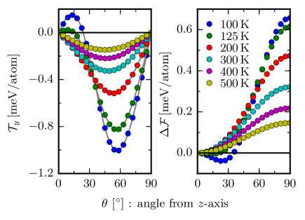
Figure 8: Angular dependence of $y$-direction torque $\mathcal{T}_{y}$ (left side) and free energy $\Delta\mathcal{F}$ (right side) at each temperature for $r_{\rm cut}=10.6\,{\rm\AA}$ and $L=4$. The gray lines on the left side show the fit of the torque data to $-\partial\Delta\mathcal{F}/\partial\theta$ in Eq. (LABEL:eq:fitting).

Figure 8 shows the $y$-direction torque $\mathcal{T}_{y}$ and free energy $\Delta\mathcal{F}$ as a function of magnetization angle $\theta$ for $L=4$ as calculated by the C-MC method. In the present paper, the directions of magnetization constrained by the C-MC method are rotated by $\theta$ around the $y$-axis. Therefore, the torque is perpendicular to the $x$-$z$ plane, i.e., both the $x$ and $z$ components of torque are zero.

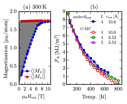
Figure 9: (left) Magnetization curve $\langle|M_{z(x)}|\rangle$ under the $z(x)$-direction of external magnetic field $H_{\rm ext}$; gray area corresponds to magnetic anisotropy energy $\mathcal{F}^{H}_{\rm A}$ in the blue solid lines on the right-hand panel. (right) $\mathcal{F}^{(H)}_{\rm A}$ for the four calculation conditions.

To verify the C-MC method, we compare the magnetic anisotropy energies $\mathcal{F}_{\rm A}$ with those given by the typical MC method, $\mathcal{F}^{H}_{\rm A}$. Here, $\mathcal{F}_{\rm A}$ is defined as $\Delta\mathcal{F}_{\rm max}-\Delta\mathcal{F}_{\rm min}$ in Fig. 8, and $\mathcal{F}^{H}_{\rm A}$ is derived from the magnetization curves as the gray area on the left of Fig. 9 (example at $T=300\,\rm K$), where $\langle|M_{x(z)}|\rangle$ is the magnetization curve under $H_{\rm ext}$ in the $x(z)$-direction. From the right of Fig. 9, we can confirm that $\mathcal{F}_{\rm A}$ is in good agreement with $\mathcal{F}^{H}_{\rm A}$, particularly in the low-temperature region, although $\mathcal{F}^{H}_{\rm A}$ tends to give an overestimate. This overestimate occurs because, at finite temperatures, the effective magnetic anisotropy of each spin decreases as a result of thermal fluctuations. When evaluating $\mathcal{F}^{H}_{\rm A}$, the thermal fluctuations are suppressed by the external field to saturate the magnetization. This suppression becomes stronger as the temperature increases, causing the overestimation to be significant in high-temperature region.

We also plot $\mathcal{F}_{\rm A}$ for other calculation conditions: $(L,\,r_{\rm cut})=$ $(4,\,3.52)$ and $(5,\,3.52)$ on the right of Fig. 9. These results show that a system size of $L=4$ is sufficient to obtain convergence in the magnetic anisotropy. Additionally, the length of $r_{\rm cut}$ affects $\mathcal{F}_{\rm A}$ at high temperatures. As mentioned in terms of spin reorientation, the magnetic anisotropy of Nd is essentially unaffected by differences in $r_{\rm cut}$. Hence, it can be regarded as that the difference between red and green lines in Fig. 9(b) occurs due to $r_{\rm cut}$ dependence of Fe anisotropy. Therefore, in high-temperature region where Fe anisotropy becomes larger than the Nd anisotropy (see Fig. 11 $A_{l}^{m_{l}}=0$ and $D^{\rm A}=0$), the effects on $\mathcal{F}_{\rm A}$ of differences in $r_{\rm cut}$ are clearly evident.

Returning to Fig. 8, we can see that for $100\,\rm K$ and $125\,\rm K$, the torque (free energy) curve attains a local maximum (minimum) at $\theta\neq 0$, which reflect the spin reorientation (shown in Fig. 4). In contrast, above $T\geq 200\,\rm K$, the local maximum (minimum) disappears and the torque (free energy) curve approaches $\propto\sin 2\theta$ ($\sin^{2}\theta$). This behavior implies that the magnetic anisotropy constant $K^{\rm A}_{1}$ becomes dominant as the temperature increases.

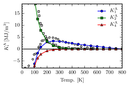
Figure 10: Anisotropy constants $K^{\rm A}_{m}$ as a function of temperature for $r_{\rm cut}=10.6\,\rm\AA$ and $L=4$. White circles and squares indicate experimental resultsDurst and Kronmüller (1986) for $K^{\rm A}_{1}$ and $K^{\rm A}_{2}$, respectively.

To clarify the temperature dependence, Fig. 10 shows the magnetic anisotropy constants $K^{\rm A}_{m}\ (m=1,2,4)$ that were calculated by fitting $\mathcal{T}_{y}$ in Fig. 8 to the torque equation:

$$\mathcal{T}_{y}(\theta,T) = -\frac{\partial}{\partial\theta}\Delta\mathcal{F}(\theta,T),$$

$$\Delta\mathcal{F}(\theta,T) = K^{\rm A}_{1}(T)\sin^{2}\theta+K^{\rm A}_{2}(T)\sin^{4}\theta+K^{\rm A}_{4}(T)\sin^{6}\theta.$$

These constants can only be calculated correctly using the C-MC method. We can confirm that $K^{\rm A}_{2}$ and $K^{\rm A}_{4}$ tend to zero and $K^{\rm A}_{1}$ becomes dominant in the region of $T>300\rm\,K$. Additionally, $K^{\rm A}_{1}$ becomes negative in the low-temperature region. This is reflected by the local minimum of $\Delta\mathcal{F}$ in Fig. 8, indicating the spin reorientation transition. The temperature dependence of $K^{\rm A}_{m}$ agrees reasonably well with previous experimental resultsHirosawa et al. (1986); Yamada et al. (1986); Durst and Kronmüller (1986) and mean field theory.Sasaki et al. (2015); Miura et al. (2015) Note that, at $T<100\,\rm K$, all of the $|K^{\rm A}_{m}|$ are significantly larger than the experimental values. For classical spin systems, this deviation in $K^{\rm A}_{m}$ (and also $M$) is finite at zero temperature on account of the infinite degrees of freedom of classical spin (for quantum spin systems, the deviations of $K^{\rm A}_{m}$ and $M$ at $T=0$ are zero).Miura et al. (2015) This explain the difference between our results and the experimental results at $T<100\,\rm K$.

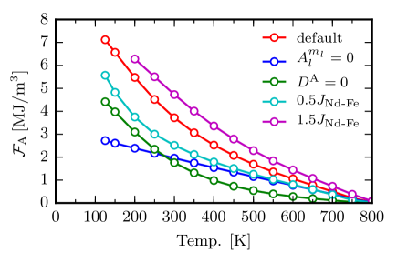
Figure 11: Comparison of the temperature dependence of magnetic anisotropy energy $\mathcal{F}_{\rm A}$ in five cases (details in text) for $r_{\rm cut}=10.6\,\rm\AA$ and $L=4$.

To examine the relationship between the exchange coupling and magnetic anisotropy, we considered various input parameter sets. Figure 11 shows the anisotropy energy $\mathcal{F}_{\rm A}$ for five cases: the same result as shown by the red lines in Fig. 9 (default), a model including only Fe magnetic anisotropy ($A_{l}^{{\color[rgb]{0,0,0}m_{l}}}=0$), a model including only Nd magnetic anisotropy ($D^{\rm A}=0$), a model with all $J_{\rm Fe\mathchar 28973\relax Nd}^{\rm ex}$ reduced by half (0.5$J_{\rm Fe\mathchar 28973\relax Nd}^{\rm ex}$), and a model with all $J_{\rm Fe\mathchar 28973\relax Nd}^{\rm ex}$ increased by half (1.5$J_{\rm Fe\mathchar 28973\relax Nd}^{\rm ex}$). In the case of $A_{l}^{{\color[rgb]{0,0,0}m_{l}}}=0$, the anisotropy energy decreases almost linearly with temperature. This behavior is a typical property of the classical Heisenberg models that include only $\sin^{2}\theta$ for the anisotropy energy. In contrast, the case of $D^{\rm A}=0$ exhibits a rapid decrease, which can be explained by the difference in the exchange coupling $\tilde{\mathcal{J}}^{\rm ex}_{\rm atom}(r_{1},r_{2})$ of Nd and Fe atoms (see Eq. (6)). We have that $\tilde{\mathcal{J}}^{\rm ex}_{\rm Fe}$ and $\tilde{\mathcal{J}}^{\rm ex}_{\rm Nd}$ for $r_{1}=0$, $r_{2}=10.6\rm\,\AA$ are $142.9\,\rm meV$ and $33.5\,\rm meV$, respectively. Here, $\tilde{\mathcal{J}}^{\rm ex}_{\rm Fe(Nd)}$ is almost given by the Fe-Fe (Nd-Fe) exchange couplings (see Fig. 3). The Nd atoms, which give the whole Nd₂Fe₁₄B system magnetic anisotropy through $\tilde{\mathcal{J}}^{\rm ex}_{\rm Nd}$, are highly susceptible to thermal fluctuations, unlike the Fe atoms, which play a key role in magnetism (such as $|\bm{M}|$ and $T_{\rm C}$). This difference in thermal susceptibility explains the rapid decrease in $\mathcal{F}_{\rm A}$ for $D^{\rm A}=0$. For the same reason, in the case of 0.5$J_{\rm Fe\mathchar 28973\relax Nd}^{\rm ex}$, which includes both $A_{l}^{{\color[rgb]{0,0,0}m_{l}}}$ and $D^{\rm A}$, $\mathcal{F}_{\rm A}$ decreases rapidly with temperature, and approaches $A_{l}^{{\color[rgb]{0,0,0}m_{l}}}=0$ at approximately $400\,\rm K$. This means that the effects of Nd magnetic anisotropy are almost wiped out by thermal fluctuations above $400\,\rm K$. However, for 1.5$J_{\rm Fe\mathchar 28973\relax Nd}^{\rm ex}$, $\mathcal{F}_{\rm A}$ is almost linear. The above discussion for Fig. 11 allows us to understand that $\tilde{\mathcal{J}}^{\rm ex}_{\rm Nd}$ (rather than $\tilde{\mathcal{J}}^{\rm ex}_{\rm Fe}$) makes a strong contribution to the magnetic anisotropy of Nd atoms, which supports the results of previous studies.Sasaki et al. (2015); Matsumoto et al. (2016)

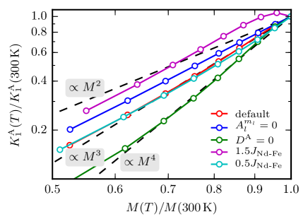
Figure 12: Relation between $K^{\rm A}_{1}(T)$ and $M(T)$ at each temperature for the same parameter sets and calculation conditions in Fig. 11. The natural logarithm is taken for both axes. The Callen–Callen law corresponds to $M(T)^{3}$, illustrated by a dashed line.

To analyze the results shown in Fig. 11 in the context of the Callen–Callen law,Callen and Callen (1963, 1966) i.e., $K^{\rm A}_{1}(T)\propto M(T)^{3}$ for $K^{\rm A}_{2}=K^{\rm A}_{4}=0$, Fig. 12 illustrates the relationship between $K^{\rm A}_{1}$ and $M$ above $300\,\rm K$. It is clear that 1.5$J_{\rm Fe\mathchar 28973\relax Nd}^{\rm ex}$ deviates from this law, because $K^{\rm A}_{2}$ is comparable to $K^{\rm A}_{1}$ at $300\,\rm K$. Varying the anisotropy terms $A_{l}^{{\color[rgb]{0,0,0}m_{l}}}$ and $D^{\rm A}$ affects these relations more than $\tilde{\mathcal{J}}^{\rm ex}_{\rm Nd}$. For $A_{l}^{{\color[rgb]{0,0,0}m_{l}}}=0$, Nd magnetization decreases rapidly with temperature, whereas Fe anisotropy decreases gradually. Hence, $K^{\rm A}_{1}/M$ tends to increase. Conversely, for $D^{\rm A}=0$, Fe magnetization slowly decreases with temperature whereas Nd anisotropy decreases rapidly, hence $K^{\rm A}_{1}/M$ tends to decrease. As above two effects happen to cancel out, the default case and 0.5$J_{\rm Fe\mathchar 28973\relax Nd}^{\rm ex}$ agree with the Callen–Callen law.

The Callen–Callen law was derived under the assumption of homogeneous ferromagnetic and single-ion anisotropy systems at temperatures far from $T_{\rm C}$. Therefore, it is natural that multi-sublattice model such as Nd₂Fe₁₄B does not follow the Callen–Callen law, which was also pointed out by using a mean field approach.Skomski et al. (2006) Additionally, in actual ferromagnetic metals that have two-ion magnetic anisotropy, the temperature dependence of magnetic anisotropy deviates from Callen–Callen law,Thiele et al. (2002); Okamoto et al. (2002); Staunton et al. (2006); Asselin et al. (2010); Kobayashi et al. (2016) such as $L1_{0}$-FePt, $K^{\rm A}_{1}(T)\propto M^{2.1}(T)$.Okamoto et al. (2002) Therefore, more detailed discussion of the temperature dependence is needed to formulate the theory for itinerant electrons and inhomogeneous systems.

III.3 Energy Barrier

Finally, we discuss the external magnetic field $H_{\rm ext}$ response of the energy barrier (activation energy)Gaunt (1986); Chantrell et al. (2000); Suess et al. (2007); Bance et al. (2015a, b) which governs the probability of magnetization reversal via the thermal fluctuation of spins. If this response can be measured experimentally,Goto et al. (2015) it would allow the magnetic coercivity mechanism to be predicted at finite temperatures.

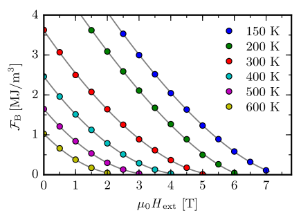
Figure 13: Height of the energy barrier, $\mathcal{F}_{\rm B}$, as a function of external magnetic field, $H_{\rm ext}$, at each temperature for $r_{\rm cut}=10.6\,\rm\AA$ and $L=4$. The gray lines illustrate the fit to Eq. (9).

Figure 13 shows the height of the energy barrier, $\mathcal{F}_{\rm B}$, when $H_{\rm ext}$ is applied opposite to the $z$-direction of $\bm{M}$. By uniformly rotating the direction of $\bm{M}$ using the C-MC method, we evaluated $\mathcal{F}_{\rm B}$; therefore, $\mathcal{F}_{\rm B}=\mathcal{F}_{\rm A}$ for $H_{\rm ext}=0$. The $H_{\rm ext}$ response of $\mathcal{F}_{\rm B}$ is generally expressed by:Gaunt (1986)

$$\mathcal{F}_{\rm B}(H_{\rm ext})=\mathcal{F}^{0}_{\rm B}(1-H_{\rm ext}/H_{0})^{n},$$ (9)

where $\mathcal{F}^{0}_{\rm B}=\mathcal{F}_{\rm B}(H_{\rm ext}=0)=\mathcal{F}_{\rm A}$, and $H_{0}$ is equal to the value of $H_{\rm ext}$ at $\mathcal{F}_{\rm B}=0$, which corresponds to the upper limit of the coercive field, $H_{c}$, under uniform rotation. For finite temperatures, and non-uniform rotation, the thermal fluctuation helps the magnetization reversal to overcome the energy barrier, and so $H_{c}$ is much lower than $H_{0}$. The exponent $n$ can take various values, such as $n=2$ for the Stoner–Wohlfarth model and $n=1$ for the weak domain-wall pinning mechanism.Gaunt (1986)

Table 2: Fitting parameters ($\mathcal{F}^{0}_{\rm B}$, $H_{0}$, $n$) at each temperature. The exponent $n^{s}_{K}$ was estimated with the single-spin model (Eq. (10)) using the anisotropy constant $K^{\rm A}_{m}$ in Fig. 10 instead of $\kappa_{m}$.

Temp. [$\rm K$]	$\mathcal{F}^{0}_{\rm B}\,[\rm MJ/m^{3}]$	$\mu_{0}H_{0}\,[\rm T]$	$n$	$\frac{K^{\rm A}_{2}}{K^{\rm A}_{1}}$	$\frac{K^{\rm A}_{4}}{K^{\rm A}_{1}}$	$n^{s}_{K}$
150	6.53	7.54	1.53	9.35	-2.55	1.56
200	5.37	6.23	1.42	1.08	-0.25	1.44
300	3.61	5.41	1.72	0.2	-0.04	1.72
400	2.46	4.44	1.90	0.05	-0.01	1.91
500	1.65	3.46	1.97	0	0	2.00
600	1.03	2.55	2.00	-0.02	0	2.05

The parameters $\mathcal{F}^{0}_{\rm B}$, $H_{0}$, and $n$ were obtained by fitting $\mathcal{F}_{\rm B}(H_{\rm ext})$ in Fig. 13, and are listed in Table 2. We can see that $n$ takes values of less than $2$ in the low-temperature region (below the room temperature, $T_{\rm R}\sim 300\,\rm K$) and approaches $2$ as the temperature increases. This reflects the fact that the magnetic anisotropy is mainly governed by the $K^{\rm A}_{1}$ term in the high-temperature region (see Fig. 10). To clarify this, we estimated the exponent $n^{s}$ by fitting from the anisotropy energy of the single-spin model, which is defined as:

$$E^{s}_{\rm A}(\theta)=\kappa_{1}\sin^{2}\theta+\kappa_{2}\sin^{4}\theta+\kappa_{4}\sin^{6}\theta+mH_{\rm ext}\cos\theta{\color[rgb]{0,0,0}.}$$

(10)

With $\kappa_{2}=\kappa_{4}=0$, this corresponds to the Stoner–Wohlfarth model. The dependence of the anisotropy constant on $n^{s}$ is plotted in Fig. 14. This figure confirms that $\kappa_{2}$ and $\kappa_{4}$ have a significant effect on $n^{s}$ for (a) $\kappa_{1}>0$, whereas $n^{s}$ is less sensitive for (b) $\kappa_{1}<0$, which corresponds to the low-temperature region below $T_{\rm sr}$ of Nd₂Fe₁₄B (see Fig. 10). Here, the deviation of $n^{s}$ given by fitting Eq. (9) becomes large when either $|\kappa_{2}|$ or $|\kappa_{4}|$ increases. Therefore, near the points where fitting error bars are large (see Fig. 14), we should pay attention to the $n^{s}$ values, which are dependent on fitting procedures.

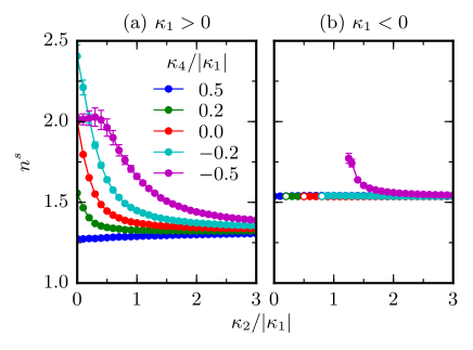
Figure 14: The exponent $n^{s}$ in the magnetic field response for the single-spin model, Eq. (10), as a function of $\kappa_{2}/|\kappa_{1}|\,(\geq 0)$ with fitting error bars ($95\,\%$ confidence) on each $\kappa_{4}/|\kappa_{1}|$ for (a) $\kappa_{1}>0$ and (b) $\kappa_{1}<0$. Energy barrier $\mathcal{F}_{B}$ disappears when $\kappa_{2}/|\kappa_{1}|$ is below each white point in (b).

Additionally, we input $K^{\rm A}_{m}$ (from Fig. 10) into $\kappa_{m}$ in Eq. (10), and estimated the exponent $n^{s}_{K}$ listed in Table 2. Despite using the single-spin model, $n^{s}_{K}$ is in good agreement with $n$, where $n$ has been evaluated on an inhomogeneous spin system such as Nd₂Fe₁₄B. This indicates that, in terms of the magnetic field response of uniform rotation, the anisotropy constants $K^{\rm A}_{m}$ are renormalized by the magnetic inhomogeneities and thermal fluctuations. For the Nd₂Fe₁₄B system, in particular, we should bear in mind that the response occurs for $n<2$ when below room temperature, $T_{\rm R}$.

IV Summary

We have constructed a realistic classical three-dimensional Heisenberg model using parameters from first-principles calculations, and investigated the magnetic properties of the Nd₂Fe₁₄B bulk system at finite temperatures. Applying the constrained Monte Carlo method to this model, from atomic-scale parameters, we evaluated macroscopic magnetic anisotropies which include correctly magnetic inhomogeneities and thermal fluctuations. Despite using many parameters from first-principles calculations (except for $A_{l}^{{\color[rgb]{0,0,0}m_{l}}}$), the model reproduced the experimentally observed spin reorientation and magnetic anisotropy constants $K^{\rm A}_{m}$.

Using this calculation system, we found that, because the exchange couplings between Nd moments and Fe spins are much smaller than those between Fe spins, the magnetic anisotropy of Nd atoms decreases more rapidly than that of Fe atoms. Additionally, owing to this magnetic inhomogeneity, the temperature dependence of $K^{\rm A}_{1}$ deviates from the Callen–Callen law, even above room temperature ($T_{\rm R}\sim 300\rm\,K$), when the Fe (Nd) anisotropy terms are removed to leave only the Nd (Fe) anisotropy. Furthermore, we also found that the exponent $n$ in the magnetic field response of barrier height is less than $2$ in the low-temperature region below $T_{\rm R}$, whereas $n$ approaches $2$ when $T>T_{\rm R}$, indicating Stoner–Wohlfarth-type magnetization rotation. This behavior reflects the fact that the magnetic anisotropy is mainly governed by the $K^{\rm A}_{1}$ term in $T>T_{\rm R}$, which is explained by the single-spin model with a renormalized $K^{\rm A}_{m}$.

We have a plan to extend the constructed framework in present paper to non-uniform magnetization reversal in finite-size particles, including the effects of the grain surfaces or grain boundaries.