Quasi-particle bands and structural phase transition of iron
from Gutzwiller Density-Functional Theory

Abstract

We use the Gutzwiller Density Functional Theory to calculate ground-state properties and bandstructures of iron in its body-centered-cubic (bcc) and hexagonal-close-packed (hcp) phases. For a Hubbard interaction $U=9\,{\rm eV}$ and Hund’s-rule coupling $J=0.54\,{\rm eV}$ we reproduce the lattice parameter, magnetic moment, and bulk modulus of bcc iron. For these parameters, bcc is the ground-state lattice structure at ambient pressure up to a pressure of $p_{\rm c}=41\,{\rm GPa}$ where a transition to the non-magnetic hcp structure is predicted, in qualitative agreement with experiment ($p_{\rm c}^{\rm exp}=10\ldots 15\,{\rm GPa}$). The calculated bandstructure for bcc iron is in good agreement with ARPES measurements. The agreement improves when we perturbatively include the spin-orbit coupling.

I Introduction

The theoretical description of the structural and electronic properties of iron poses an interesting but difficult problem. Since iron is an essential element in the inner core of the earth it is desirable to know its phase diagram over a wide temperature and pressure range. However, basic calculations at ambient pressure and zero temperature reveal the intricacy of the iron problem. Ab-initio calculations with Density Functional Theory (DFT) in the Local Density Approximation, DFT(LDA), predict a wrong lattice structure for the ground state, namely face-centered-cubic (fcc) or hexagonal-close-packed (hcp). PhysRevLett.54.1852 ; PhysRevB.67.214518 Employing DFT with a Generalized Gradient Approximation, DFT(GGA), standard bandstructure theory recovers the experimentally observed ferromagnetic body-centered-cubic (bcc) structure and the bcc-hcp transition. PhysRevB.50.6442 ; PhysRevB.58.5296 Using the standard GGA functional of Perdew, Burke, and Ernzerhof (PBE), PBE a good description of the lattice parameter, magnetization, and compressibility of iron, cobalt, and nickel is obtained. PhysRevB.60.791 ; Taiwanesen However, as for nickel, 1367-2630-16-9-093034 both DFT functionals lead to a $d$-electron bandwidth that is too large and quasi-particle masses at the Fermi edge that are too small in comparison with experiment. PhysRevLett.110.117206 This indicates that neither of the DFT functionals takes into account the correlations among the $3d$ electrons in an optimal way.

Coulomb correlations for electrons in narrow bands are often modeled by a purely local, Hubbard-type interaction. Hubbard1963 ; Gutzwiller1963 ; Hubbard1964 ; Gutzwiller1964 Typically, the effective atomic interactions are parameterized by an intra-orbital Hubbard interaction $U$ and a Hund’s-rule coupling $J$. Unfortunately, Hubbard models pose a notoriously difficult many-body problem.

Over the past three decades, two many-body approaches emerged that permit a treatment of Hubbard-type interactions in the limit of infinite lattice coordination number in combination with DFT. First, the Dynamical Mean-Field Theory (DMFT) RevModPhys.78.865 ; VollhardtAnnalen maps the problem onto a single-impurity model. The spectral function of the (multi-orbital) single-impurity model is calculated numerically, typically using Quantum Monte-Carlo. RevModPhys.83.349 With DMFT(QMC), iron’s structural and magnetic transitions at temperatures $T>1000\,{\rm K}$ were studied in Ref. [0953-8984-26-37-375601, ] (and references therein), and the equation-of-state for the bcc-hcp phase transition was investigated in Ref. [PhysRevB.90.155120, ]. Second, the Gutzwiller many-body wavefunction is combined with DFT(LDA) to treat local interactions variationally (‘LDA+Gutzwiller’, ‘Gutzwiller-DFT’), see Refs. [Ho2008, ; Deng2008, ; Deng2009, ; Wang2008, ; Wang2010, ; Weng2011, ; Yao2011a, ; PhysRevB.84.205124, ; PhysRevB.85.035133, ; PhysRevB.87.045122, ; PhysRevLett.111.196801, ; PhysRevB.90.161104, ; PhysRevB.89.165122, ; 1367-2630-16-9-093034, ; PhysRevX.5.011008, ]. Recently, the LDA+Gutzwiller approach was applied to a number of transition metals including nickel, iron, and iron pnictides. PhysRevB.90.125102 ; Deng2009 ; Wang2010 ; Yao2011a ; Schickling2012

The DMFT becomes exact in infinite dimensions but the numerical effort is quite considerable which often makes further simplifications of the interactions advisable. 0953-8984-26-37-375601 Moreover, the computational demands limit the studies to elevated temperatures and prohibits an extensive scan in the $(U,J)$ parameter space. On the other hand, the Gutzwiller approach is a variational method at zero temperature and therefore best suited for the calculation of ground-state properties such as the lattice parameter, magnetization, and bulk modulus. Dynamical properties, however, can only be described within the quasi-particle picture, i.e., the method provides a bandstructure but no quasi-particle lifetimes. Since the Gutzwiller-DFT is computationally much cheaper than DFT(LDA-DMFT), it permits a survey of the $(U,J)$ parameter space for iron.

In this study, we present comprehensive results for iron obtained from the LDA+Gutzwiller method. We obtain the experimental values for the lattice parameter, magnetization, and compressibility, and provide a qualitatively correct description of the structural transition from bcc to hcp iron under pressure. When we take spin-orbit effects into account perturbatively, we obtain a good agreement with ARPES measurements of the quasi-particle bandstructure. PhysRevB.72.155115

Our work is structured as follows. In Sect. II, we summarize the Gutzwiller-DFT that was derived in detail in Ref. [1367-2630-16-9-093034, ]; here, we generalize it to the case of more than one atom per unit cell. In Sect. III we discuss our results for the ground-state properties of iron. In Sect. IV, we present the respective quasi-particle bandstructures and compare them to ARPES data for bcc iron. Conclusions, Sect. V, close our presentation.

II Method

The Gutzwiller-DFT and the minimization algorithm which we use in this work have been discussed in detail in Refs. [1367-2630-16-9-093034, ] and [Buenemann-2012-b, ]. Therefore we will only summarize the main ideas of these methods in the present section and focus on some particular aspects that are relevant in our calculations for iron.

II.1 Gutzwiller-DFT

Instead of a single-particle reference system that leads to the standard Kohn-Sham equations, the Gutzwiller-DFT employs a many-particle reference system. It explicitly takes into account the local Coulomb interaction (on lattice sites ${\mathbf{R}}$)

$$\hat{V}_{\rm loc} = \sum_{{\mathbf{R}}}\hat{V}_{\rm loc}({\mathbf{R}})\;,$$ (1)

$$\hat{V}_{\rm loc}({\mathbf{R}}) = \sum_{\gamma_{1},\ldots,\gamma_{4}}U^{\gamma_{1},\gamma_{2}}_{\gamma_{3},\gamma_{4}}\,\hat{c}_{{\mathbf{R}},\gamma_{1}}^{+}\hat{c}_{{\mathbf{R}},\gamma_{2}}^{+}\hat{c}_{{\mathbf{R}},\gamma_{3}}^{\vphantom{+}}\hat{c}_{{\mathbf{R}},\gamma_{4}}^{\vphantom{+}}$$ (2)

in those spin-orbital states $\phi_{{\mathbf{R}},\gamma}({\mathbf{r}})\equiv\phi_{{\mathbf{R}},c,\sigma}({\mathbf{r}})$ which are deemed to be strongly correlated. In our iron calculations these are the $e_{g}$ and $t_{2g}$ orbitals of the $3d$ shell. The explicit form of the operator $\hat{V}_{\rm loc}({\mathbf{R}})$ for $d$-orbitals is given in Ref. [1367-2630-16-9-093034, ], see also appendix A. As also shown in that work, one obtains the following ‘Hubbard density functional’ for the many-particle reference system

$$E_{\rm H}\left[\left\{n_{\sigma}({\mathbf{r}})\right\}\right] = K_{\rm H}\left[\left\{n_{\sigma}({\mathbf{r}})\right\}\right]+U\left[\left\{n_{\sigma}({\mathbf{r}})\right\}\right]$$ (3)

$$+V_{\rm Har}\left[\left\{n_{\sigma}({\mathbf{r}})\right\}\right]$$

$$+V_{\rm loc}\left[\left\{n_{\sigma}({\mathbf{r}})\right\}\right]-V_{\rm dc}\left[\left\{n_{\sigma}({\mathbf{r}})\right\}\right]$$

$$+E_{\rm H,xc}\left[\left\{n_{\sigma}({\mathbf{r}})\right\}\right]\;,$$

where $E_{\rm H,xc}\left[\left\{n_{\sigma}({\mathbf{r}})\right\}\right]$ is the exchange-correlation functional, see Sect. II.3, and

$$U\left[\left\{n_{\sigma}({\mathbf{r}})\right\}\right] = \sum_{\sigma}\int{\rm d}{\mathbf{r}}U({\mathbf{r}})n_{\sigma}({\mathbf{r}})\;,$$ (4)

$$V_{\rm Har}\left[\left\{n_{\sigma}({\mathbf{r}})\right\}\right] = \sum_{\sigma,\sigma^{\prime}}\int\!\!\int{\rm d}{\mathbf{r}}{\rm d}{\mathbf{r}}^{\prime}V({\mathbf{r}}-{\mathbf{r}}^{\prime})n_{\sigma}({\mathbf{r}})n_{\sigma^{\prime}}({\mathbf{r}}^{\prime})\;,$$

$$K_{\rm H}\left[\left\{n_{\sigma}({\mathbf{r}})\right\}\right] = \langle\Psi_{\rm H,0}^{(n)}|\hat{H}_{\rm kin}|\Psi_{\rm H,0}^{(n)}\rangle\,,$$ (6)

$$V_{\rm loc/dc}\left[\left\{n_{\sigma}({\mathbf{r}})\right\}\right] = \langle\Psi_{\rm H,0}^{(n)}|\hat{V}_{\rm loc/dc}|\Psi_{\rm H,0}^{(n)}\rangle\;.$$ (7)

Here, we introduced the periodic potential $U({\mathbf{r}})$ of the nuclei and the two-particle Coulomb interaction $V({\mathbf{r}}-{\mathbf{r}}^{\prime})$. The state $|\Psi_{\rm H,0}^{(n)}\rangle$ minimizes, by definition, the expectation value of the Hamiltonian

$$\hat{H}_{\rm H}=\hat{H}_{\rm kin}+\hat{V}_{\rm loc}-\hat{V}_{\rm dc}\;,$$ (8)

for a given (and fixed) particle density $n_{\sigma}({\mathbf{r}})$. Finally, the ‘double-counting operator’ $\hat{V}_{\rm dc}$ and the corresponding functional $V_{\rm dc}\left[\left\{n_{\sigma}({\mathbf{r}})\right\}\right]$ account for the fact that the local Coulomb interaction between electrons in the correlated orbitals is already included in the Hartree energy and the exchange-correlation functional. Unfortunately, there is no systematic way to derive $\hat{V}_{\rm dc}$ for a given local Hamiltonian $\hat{V}_{\rm loc}$. We work with the widely used form of the double-counting functional, PhysRevB.44.943 ; PhysRevB.52.R5467 ; RevModPhys.78.865 ; Deng2009 see appendix A.

In contrast to the corresponding Kohn-Sham functional, $E_{\rm H}\left[\left\{n_{\sigma}({\mathbf{r}})\right\}\right]$ cannot be minimized without further approximations. In fact, it cannot even be evaluated because $\hat{H}_{\rm H}$ is a many-particle Hamiltonian. We therefore use Gutzwiller wavefunctions for the evaluation of (6) and (7). They are defined as

$$|\Psi_{\rm G}\rangle = \hat{P}_{\rm G}|\psi_{0}\rangle\;,$$ (9)

$$\hat{P}_{\rm G} = \prod_{{\mathbf{R}}}\sum_{\Gamma,\Gamma^{\prime}}\lambda_{\Gamma,\Gamma^{\prime}}({\mathbf{R}})\hat{m}_{{\mathbf{R}};\Gamma,\Gamma^{\prime}}\;,$$ (10)

where $|\psi_{0}\rangle$ is a single-particle product state, and $\lambda_{\Gamma,\Gamma^{\prime}}({\mathbf{R}})$ are the elements of the variational parameter matrix $\tilde{\lambda}({\mathbf{R}})$. We further introduced the eigenstates $|\Gamma\rangle_{{\mathbf{R}}}$ of $\hat{V}_{\rm loc}({\mathbf{R}})$ and the operator

$$\hat{m}_{{\mathbf{R}};\Gamma,\Gamma^{\prime}}\equiv|\Gamma\rangle_{{\mathbf{R}}}{}_{{\mathbf{R}}}\langle\Gamma^{\prime}|\;.$$ (11)

In our calculations for iron, we work with a diagonal and lattice-site independent variational parameter matrix $\lambda_{\Gamma,\Gamma^{\prime}}({\mathbf{R}})=\delta_{\Gamma,\Gamma^{\prime}}\lambda_{\Gamma}$, i.e., our energy functional depends on $n_{\Gamma}=2^{10}=1024$ variational parameters $\lambda_{\Gamma}$. Note that non-diagonal variational parameters do not substantially change the results in our high-symmetry cubic situation in the absence of spin-orbit coupling. Moreover, we do not find it necessary to implement symmetry relations among the 1024 variational parameters. This has been done in Ref. [PhysRevB.90.125102, ] where also non-diagonal variational parameters $\lambda_{\Gamma,\Gamma^{\prime}}$ were taken into account.

The evaluation of Eqs. (6) and (7) still is a difficult many-particle problem. It can be solved in the limit of infinite spatial dimensions where one obtains an analytical energy functional. Using this energy functional in calculations on finite-dimensional systems, as done in this work, is usually denoted as the ‘Gutzwiller approximation’ to the energy functional $E_{\rm H}\left[\left\{n_{\sigma}({\mathbf{r}})\right\}\right]$.

We shall not repeat here the details of the Gutzwiller approximation or the structure of the resulting energy functional because it has been thoroughly discussed in earlier work. Obviously, one obtains a functional of the form

$$E_{\rm H}=E_{\rm H}(|\psi_{0}\rangle,\{\lambda_{\Gamma}\})$$ (12)

that depends on the single-particle state $|\psi_{0}\rangle$ and the variational parameters $\lambda_{\Gamma}$. The minimization of the energy functional with respect to $|\psi_{0}\rangle$ leads to an effective single-particle Schrödinger equation for $|\psi_{0}\rangle$. This ‘Gutzwiller–Kohn-Sham equation’ is the equivalent to the Kohn-Sham equation in ordinary DFT calculations and is solved by an adapted version of the open source Quantum ESPRESSO code. 0953-8984-21-39-395502

For the minimization with respect to the variational parameters $\lambda_{\Gamma}$ (‘inner minimization’), we use an algorithm whose elements were discussed in Ref. [Buenemann-2012-b, ]. The new feature of our present calculations comes from the fact that in hcp iron we have a unit cell with two iron atoms. Since both iron sites have the same point symmetry one could actually use the existing minimization algorithm. Buenemann-2012-b For later use and testing purposes, however, we developed a code that is capable to carry out the inner minimization for a large number of in-equivalent correlated atoms per unit cell. We explain this algorithm in the following Sect. II.2.

II.2 Inner minimization for systems with multiple atoms per unit cell

Let $l=1,\ldots,n_{l}$ be the label for the $n_{l}$ atoms in the unit cell and $\tilde{\lambda}^{l}$ the corresponding matrices of variational parameters. Then, for a translationally invariant system, the energy functional of the Gutzwiller approximation has the form

$$E(\{\tilde{\lambda}^{l}\}) = \sum_{l}V_{l;{\rm loc}}(\tilde{\lambda}^{l})$$

$$+\sum_{l}\!\sum_{\gamma_{1},\gamma_{2}}q^{l;\gamma_{2}}_{\gamma_{1}}(\tilde{\lambda}^{l})K^{l}_{\gamma_{1},\gamma_{2}}+{\rm c.c.}$$

$$+\sum_{l,l^{\prime}}\!\sum_{\gamma_{1},\ldots,\gamma_{4}}q^{l;\gamma_{2}}_{\gamma_{1}}(\tilde{\lambda}^{l})\left(q^{l^{\prime};\gamma_{4}}_{\gamma_{3}}(\tilde{\lambda}^{l^{\prime}})\right)^{*}I^{l,l^{\prime}}_{\gamma_{1},\gamma_{2},\gamma_{3},\gamma_{4}}\,.$$

The third line describes the hopping of electrons between correlated orbitals while the second line includes all contributions from hopping processes into non-correlated orbitals. During the inner minimization, the tensors $K^{l}_{\gamma_{1},\gamma_{2}}$ and $I^{l,l^{\prime}}_{\gamma_{1},\gamma_{2},\gamma_{3},\gamma_{4}}$ are just numbers that result from the solution of the Gutzwiller–Kohn-Sham equation. Note that in our calculations for iron, the renormalization matrices $q^{l;\gamma_{2}}_{\gamma_{1}}$ are real and diagonal, $q^{l;\gamma_{2}}_{\gamma_{1}}=\delta_{\gamma_{1},\gamma_{2}}q^{l;\gamma_{1}}_{\gamma_{1}}$, which simplifies the energy functional considerably.

The energy functional (II.2) needs to be minimized with respect to all matrices $\tilde{\lambda}^{l}$. Even with our diagonal Ansatz for $\tilde{\lambda}^{l}$, however, the total number of variational parameters $n_{\rm tot}=n_{\Gamma}\times n_{l}$ would become prohibitively large if we tried to minimize straightforwardly systems with different atoms in the unit cell. Instead of minimizing (II.2) directly with respect to all matrices $\tilde{\lambda}^{l}$ simultaneously, we therefore use the following scheme.

• Start with some initial values for the matrices $\tilde{\lambda}^{l}_{0}$ and the corresponding renormalization matrices $q^{l;\gamma_{2}}_{\gamma_{1};0}\equiv q^{l;\gamma_{2}}_{\gamma_{1}}(\tilde{\lambda}^{l}_{0})$, e.g., the values in the non-interacting limit.

• Minimize the $n_{l}$ individual energy functionals

  $$E_{l}(\tilde{\lambda}^{l}) = V_{l;{\rm loc}}(\tilde{\lambda}^{l})$$

  $$+\sum_{\gamma_{1},\gamma_{2}}q^{l;\gamma_{2}}_{\gamma_{1}}(\tilde{\lambda}^{l})K^{l}_{\gamma_{1},\gamma_{2}}+{\rm c.c.}$$

  $$+\frac{1}{2}\sum_{l^{\prime}}\sum_{\gamma_{1},\ldots,\gamma_{4}}q^{l;\gamma_{2}}_{\gamma_{1}}(\tilde{\lambda}^{l})\left(q^{l^{\prime};\gamma_{4}}_{\gamma_{3};0}\right)^{*}I^{l,l^{\prime}}_{\gamma_{1},\gamma_{2},\gamma_{3},\gamma_{4}}$$

  with respect to $\tilde{\lambda}^{l}$, e.g., by means of the algorithm introduced in Ref. [Buenemann-2012-b, ].

• If the matrices $\tilde{\lambda}^{l}_{1}$ minimize the $n_{l}$ functionals (LABEL:44), set $\tilde{\lambda}^{l}_{0}=\tilde{\lambda}^{l}_{1}$ and go back to step (i) until a converged solution has been reached.

In our actual calculations, the band optimization (Gutzwiller–Kohn-Sham equations for $|\psi_{0}\rangle$) and of the local parameters (inner minimization) are not separated. After an update of the matrices $\tilde{\lambda}^{l}$ in step (ii), the matrices $q^{l;\gamma_{2}}_{\gamma_{1}}$ are recalculated. Then, the Gutzwiller–Kohn-Sham equation is solved again to arrive at new values for the tensors $K^{l}_{\gamma_{1},\gamma_{2}}$ and $I^{l,l^{\prime}}_{\gamma_{1},\gamma_{2},\gamma_{3},\gamma_{4}}$ in eq. (LABEL:44). Typically, we need 10 to 15 iterations of the combined cycle of band optimization and inner minimization to reach a converged minimum.

II.3 Computational details

Our work is based on the open-source plane-wave pseudopotential code Quantum ESPRESSO. 0953-8984-21-39-395502 We implemented the routines necessary for the Gutzwiller-DFT, as described previously in Ref. [1367-2630-16-9-093034, ], see the supplemental material for further information. For the Gutzwiller–Kohn-Sham calculations we used the LDA exchange-correlation functional of Perdew and Zunger for $E_{\rm H,xc}\left[\left\{n_{\sigma}({\mathbf{r}})\right\}\right]$; note that our calculations start from the local spin-density approximation (LSDA) so that we recover the results from DFT(LSDA) for $U=J=0$. For comparison, we also performed GGA calculations based on the Perdew-Burke-Ernzerhof functional. To model the electron-core interaction, we employed ultrasoft pseudo potentials from the standard Quantum ESPRESSO distribution with non-linear core corrections. These are Fe.pz-nd-rrkjus.UPF (LDA), and Fe.pbe-spn-rrkjus_psl.0.2.1.UPF (Fe.rel-pbe-spn-rrkjus_psl.0.2.1.UPF) for (scalar) relativistic GGA calculations. The GGA pseudopotentials yield equilibrium lattice constants ($a_{\rm GGA}=5.39a_{\rm B}$), magnetic moments ($m_{\rm GGA}=2.25\mu_{B}$), and electronic structure in excellent agreement with previous full-potential calculations. PhysRevB.72.155115

In Gutzwiller-DFT, we find that a very accurate integration over ${\bf k}$-space is needed for a proper convergence. Therefore, integrations over the Brillouin zone are performed using the tetrahedron method. For bcc iron, we use at least 624 ${\mathbf{k}}$-points in the irreducible part of the Brillouin zone. For non-magnetic hcp, we work with 729 inequivalent ${\mathbf{k}}$-points. For all calculations a wave cutoff of $60\,\mathrm{Ry}$ was set, and a charge-density cutoff of $600\,\mathrm{Ry}$.

For the construction of the $3d$-orbitals we employ the program package poormanwannier that is part of the standard Quantum ESPRESSO distribution. We generate Wannier functions using a very large energy window of 90 eV around the Fermi energy and the resulting $3d$ orbitals are very close to localized $3d$ orbitals. More details on the choice of the energy window and implementations are given in Sect. III A in the supplemental material. suppmat In the following we denote our implementation of the LDA+Gutzwiller scheme as ‘Gutzwiller-DFT’.

III Ground-state properties

III.1 Adjustment of the Coulomb parameters

The Gutzwiller-DFT is not a fully ab-initio method. The Coulomb interaction between the $3d$-electrons is parameterized by the Hubbard interaction $U$ and the Hund’s-rule coupling $J$. In this work, we choose to adjust these two parameters such that the Gutzwiller-DFT reproduces the experimental values for the lattice parameter $a$ and the magnetization $m$; see our discussion Sect. III.1.3.

The DFT(LDA) predicts a fcc or hcp crystal structure as ground state for iron at ambient pressure. PhysRevLett.54.1852 ; PhysRevB.67.214518 Therefore, we do not show the results for $U=J=0$ in the following. This serious flaw of DFT(LDA) is easily overcome with LDA+Gutzwiller, and also in DFT(GGA) where $a_{\rm GGA}\approx 5.36\,a_{\rm B}$ and $m\approx 2.2\,\mu_{\rm B}$ are obtained. PhysRevB.50.6442 ; PhysRevB.58.5296 For local interactions as small as $U\geq 1.0\,\mathrm{eV}$ and $J=0.06U$, Gutzwiller-DFT finds the experimentally observed ferromagnetic bcc lattice structure. Therefore, the correct ground-state structure dominates the $(U,J)$ phase diagram, and it is straightforward to search for the optimal Hubbard interaction $U$ and Hund’s-rule coupling $J$, as was done for nickel previously. 1367-2630-16-9-093034

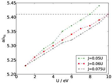
Figure 1: Cubic lattice parameter $a(U,J)$ for bcc iron in units of the Bohr radius $a_{\rm B}=0.529\,\hbox{\AA}$ as a function of the Hubbard interaction $U$ for $J/U=0.05,0.06,0.075$. The horizontal dashed line indicates the experimental value $a^{\rm exp}=5.42a_{\rm B}=2.87\,\hbox{\AA}$.

III.1.1 Lattice parameter

In Fig. 1 we display the bcc lattice parameter $a(U,J)$ as a function of $U$ for various ratios $J/U$. The horizontal dashed line indicates the experimental value, $a^{\rm exp}=5.42a_{\rm B}=2.87\,\hbox{\AA}$. PhysRevB.82.132409 As also seen in nickel, 1367-2630-16-9-093034 the lattice parameter increases monotonously as a function of the Hubbard interaction. This effect is desired because the DFT(LDA) considerably underestimates the lattice parameter for iron.

The influence of the Hubbard interaction is readily understood. The Coulomb repulsion weakens the contribution of the $3d$-electrons to the metallic binding so that the crystal is less tightly bound; the crystal volume increases as a function of the Coulomb repulsion. Figure 1 shows that the Hund’s-rule coupling $J$ counteracts the Hubbard interaction $U$. The slope of $a(U,J)$ as a function of $U$ becomes smaller for larger $J$. This indicates that the Hund’s-rule coupling $J$ in iron has a tendency to increase the electrons’ itineracy, see below.

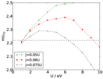
Figure 2: Magnetization $m(U,J)$ in units of Bohr magneton $\mu_{\rm B}$ as a function of the Hubbard interaction $U$ for $J/U=0.05,0.06,0.075$. The horizontal dashed line indicates the experimental value $m=2.22\mu_{\rm B}$.

III.1.2 Magnetization

In Fig. 2 we show the ordered magnetic moment $m(U,J)$ as a function of the Hubbard interaction $U$ for the previously used ratios $J/U=0.05,0.06,0.075$. The horizontal dashed line indicates the experimental value, $m^{\rm exp}=2.22\mu_{\rm B}$. Dananetal The ordered magnetic moment $m$ is calculated from the particle densities $n_{\sigma}({\mathbf{r}})$ as

$$m/\mu_{\rm B}=\int d{\mathbf{r}}[n_{\uparrow}({\mathbf{r}})-n_{\downarrow}({\mathbf{r}})]\,,$$ (15)

where we used $g=2$ as the electrons’ gyromagnetic factor.

It is important to note that the DFT(LDA) predicts a large magnetization, i.e., iron is a band ferromagnet in DFT(LSDA). Figure 2 shows that the Coulomb corrections due to the intra-atomic correlations in the $3d$-shell amount to only 10% of the magnetization. Indeed, in the parameter regime shown in Fig. 2, we have $2.0\mu_{\rm B}<m<2.4\mu_{\rm B}$ for $1\,{\rm eV}\leq U\leq 9\,{\rm eV}$ and $J/U=0.06,0.075$.

Since the Coulomb correlations in the $3d$-shell are not the primary cause for magnetism, the magnetization $m(U,J)$ does not show a simple dependence on the Hubbard interaction $U$ in combination with the Hund’s-rule coupling $J$. In iron, for vanishing Hund’s-rule coupling, $J/U=0$, we find that the magnetization increases as a function of $U$, as also seen in LDA+$U$. This is the usual Stoner mechanism: in a magnetized system there is less Coulomb energy to be paid, at the price of a loss in kinetic energy. When we increase $U$, the energy balance is shifted towards the exchange-energy gain so that the magnetization increases.

Within the Gutzwiller-DFT, the Hund’s-rule coupling leads to the rather unexpected behavior seen in Fig. 2. For fixed $U$, an increase of the Hund’s-rule coupling $J$ leads to a decrease of the magnetization $m(U,J)$. Such a behavior was observed previously in iron, Deng2009 and also in nickel. 1367-2630-16-9-093034 Moreover, the influence of the Hund’s-rule coupling is not small. Indeed, as seen in Fig. 2, it leads to a parabolic downturn of $m(U,J)$ as a function of $U$ for fixed $J/U$. We shall discuss the effect of the Hund’s-rule coupling in more detail in Sect. III.2.3.

Using the information in figures 1 and 2 we can determine the optimal values for the interaction parameters. For $U_{\rm opt}=9.0\,{\rm eV}$ and $J_{\rm opt}=0.54\,{\rm eV}$, we obtain good results for the lattice parameter and the magnetic moment, $a_{\rm opt}=a(U_{\rm opt},J_{\rm opt})=5.39a_{\rm B}=2.85\,\hbox{\AA}$ and $m_{\rm opt}=m(U_{\rm opt},J_{\rm opt})=2.24\mu_{\rm B}$, that agree very well with the experimental values. In the rest of paper we refer to the parameter set $(U_{\rm opt},J_{\rm opt})$ as our ‘optimal’ atomic parameters.

III.1.3 Size of optimal atomic parameters

Before we proceed, we briefly comment on our optimal Coulomb parameters because they are substantially larger than parameters used in other studies for iron. 0953-8984-26-37-375601 ; PhysRevB.81.045117 ; PhysRevLett.106.106405 ; Leonov2014 ; PhysRevLett.87.067205 In most previous studies, the values $U=2\,{\rm eV}\ldots 3\,{\rm eV}$ and $J=0.8\,{\rm eV}\ldots 1.0\,{\rm eV}$ are used, e.g., to describe the high-temperature regime with the transition from fcc iron to bcc iron and the Curie transition from non-magnetic to magnetic bcc iron, while more recent LDA+DMFT studies employ larger values, $\bar{U}=4.3\,{\rm eV}$, $\widetilde{J}=1.0\,{\rm eV}$. PhysRevB.90.155120 In all cases, the explored parameter regime appears to be quite different from ours.

First of all, we note that the large spread of values of $(U,J)$ in the literature is due to the strong sensitivity of these parameters to the energy window used for projecting, or downfolding, the full electronic structure to an effective many-body model. PhysRevB.80.155134 It is well known that the bare Hubbard parameters $U$ are of the order of 20 eV, or larger. Hubbard1963 They apply for instantaneous charge excitations of an isolated atom, which are strongly screened in a solid. In Fe, for example, the screening reduces $U$ to $\sim$ 3 eV for $d$-only models. Schickling2011 ; Schickling2012 Our self-consistent DFT method is based on a projective technique to construct Wannier functions. In the present calculations, we chose a large energy window, which ensures a very good localization of the Fe $3d$ orbitals, and a minimal dependence of the basis set on atomic positions. This large energy window translates into larger values of $U,J$. PhysRevB.74.125106 Other calculations can typically afford to retain fewer bands.

Second, we note that the Hubbard-$U$ in our treatment parameterizes the interaction of two electrons in the same orbital, see appendix A. In other approaches, this quantity describes some orbital average. For example, Pourovskii et al. PhysRevB.90.155120 use the Slater-Condon parameter $F^{(0)}=\bar{U}$, where $\bar{U}=(U+4U^{\prime})/5$, see eq. (26), and $U^{\prime}=A-B+C=U-2J$ is the inter-orbital Coulomb repulsion. Naturally, the intra-orbital $U$ is larger than an average over intra-orbital and inter-orbital Coulomb repulsions. Likewise, we work with the average Hund’s-rule coupling $J=5B/2+C$, see eq. (23), whereas $\widetilde{J}\equiv(F^{(2)}+F^{(4)})/14=7B/2+7C/5=7J/5$. PhysRevB.90.155120 Therefore, $F^{(0)}=4.3\,{\rm eV}$ and $\widetilde{J}=1.0\,{\rm eV}$ correspond to $J=0.71\,{\rm eV}$ and $U=\bar{U}+8\widetilde{J}/7=5.4\,{\rm eV}$ with $J/U=0.13$. We note in passing that we work with $C/B=4$ whereas others use $F^{(2)}/F^{(4)}=8/5$ which corresponds to $C/B=175/47\approx 3.7$. PhysRevB.42.5459

Lastly, in our Gutzwiller calculations, we use parameters such as $U$ and $J$ to ‘match’ selected experimental quantities. In this way, we compensate approximations in the model setup, e.g., the neglect of non-local correlations in Hubbard-type models, and in the model analysis, e.g., the limit of infinite dimensions or an approximate variational ground state. For example, in Gutzwiller calculations, the optimal Coulomb parameters must be chosen somewhat smaller when the full atomic interaction is replaced by density-density interactions only. Schickling2012 Similarly, larger $U$-values are found to be optimal when the impurity solver in Quantum-Monte-Carlo is rotationally invariant. 0953-8984-26-37-375601 In the following we will show that our optimal atomic parameters lead to a good agreement with experiment. In particular, our substantial Hubbard interaction leads to noticeable bandwidth renormalizations and an increase of the quasi-particle masses at the Fermi energy, as seen in experiment. PhysRevB.72.155115 ; PhysRevLett.103.267203

We note that the atomic parameters for our study of iron resemble those used in recent LDA+Gutzwiller studies by Deng et alii, Deng2008 ; Deng2009 and our results agree quite well; on the other hand, we do not agree with Borghi et al. PhysRevB.90.125102 who advocate small Hubbard interactions in their LDA+Gutzwiller work; however, as discussed in the following, there are sizable discrepancy between their and our results already at the DFT(LDA) level, and this prevents a detailed comparison.

III.2 Physical properties within Gutzwiller-DFT

After fixing the parameters, we are in the position to test the Gutzwiller-DFT against independent experimental observations. Here, we choose the bulk modulus and the transition from ferromagnetic bcc iron to non-magnetic hcp iron. Furthermore, we discuss the local occupancies in more detail to elucidate the unexpected effect of the Hund’s-rule coupling on the magnetization seen in Fig. 2.

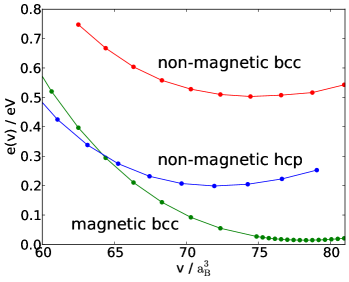
Figure 3: Energy per atom $e(v)$ in units of eV as a function of the unit-cell volume $v$ in units of $a_{\rm B}^{3}$ for non-magnetic and ferromagnetic bcc iron and non-magnetic hcp iron at $U=9\,{\rm eV}$ and $J=0.54\,{\rm eV}$ and ambient pressure. The energies are shifted by the same constant amount.

III.2.1 Bulk modulus

In Fig. 3 we show the ground-state energy per atom, $e(v)=E(V)/N$, as a function of the unit-cell volume $v=V/N=a^{3}/2$ in the vicinity of the optimal value $v_{0}=a_{\rm opt}^{3}/2=78.3a_{\rm B}^{3}=11.6\,\hbox{\AA}^{3}$ with $a_{\rm opt}=5.39a_{\rm B}=2.85\,\hbox{\AA}$. The bulk modulus at zero temperature is defined as the second-derivative of the ground-state energy $E(V)$ with respect to the volume,

$$B=v_{0}\left.\frac{{\rm d}^{2}e(v)}{{\rm d}v^{2}}\right|_{v=v_{0}}\;.$$ (16)

This implies the Taylor expansion $e(v)=e(v_{0})+(Bv_{0}/2)(v/v_{0}-1)^{2}+\ldots$ for the ground-state energy (Birch-Murnaghan fit). Therefore, we find the bulk modulus from the curvature of $e(v)$ near $v=v_{0}$.

In Gutzwiller-DFT we find a bulk modulus of $B=165\,{\rm GPa}$, in very good agreement with the experimental value, $B^{\rm exp}=(170\pm 4)\,{\rm GPa}$. JGRB:JGRB5666 ; PhysRevB.82.132409 The LDA+Gutzwiller value substantially improves the DFT(LDA) value of $B^{\rm LDA}=227\,{\rm GPa}$, it is slightly better than the values from DFT(GGA) studies, $B^{\rm GGA}=(190\pm 10)\,{\rm GPa}$, PhysRevB.82.132409 and agrees with the value obtained in DMFT calculations, $B^{\rm DMFT}=168\,{\rm GPa}$. PhysRevB.90.155120

III.2.2 Pressure-induced transition from bcc to hcp iron

Figure 3 shows that the bcc structure is only stable because it is ferromagnetic. Andersenphysica By reducing the volume by applying external pressure, a first-order structural transition is observed at a pressure of $p_{\rm c}^{\rm exp}=10\ldots 15\,{\rm GPa}$ at room temperature, bcc-to-hcp-first together with the concomitant electronic and magnetic changes. Iota ; PhysRevLett.110.117206

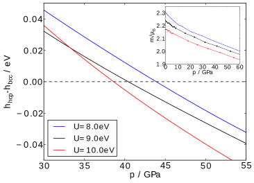
Figure 4: Enthalpy difference per atom $h_{\rm hcp}-h_{\rm bcc}$ in units of eV between non-magnetic hcp iron and ferromagnetic bcc iron as a function of applied pressure $p$ for $U=8.0,9.0,10\,{\rm eV}$ and $J/U=0.06$. Inset: magnetization as a function of pressure.

In Fig. 4 we plot the enthalpy difference per atom between the non-magnetic hcp lattice and the ferromagnetic bcc lattice as a function of applied pressure for $U=8.0,9.0,10\,{\rm eV}$ for fixed ratio $J/U=0.06$. For our optimal parameter set ($U=9.0\,{\rm eV},J=0.06U=0.54\,{\rm eV})$ we obtain $p_{\rm c}=41\,{\rm GPa}$ as critical pressure at zero temperature, in qualitative agreement with experiment. The critical parameter only slightly depends on the value of $U$ in the vicinity of $U=U_{\rm opt}$. We find at $J/U=0.06$ that $p_{\rm c}$ decreases as a function of $U$, from $p_{\rm c}=44\,{\rm GPa}$ for $U=8.0\,{\rm eV}$ down to $p_{\rm c}=38\,{\rm GPa}$ for $U=10\,{\rm eV}$. Therefore, the transition at positive pressures is a robust feature in Gutzwiller-DFT. We note in passing that the critical pressure sensitively depends on the ratio $J/U$. For $U=9\,{\rm eV}$, we find $p_{\rm c}=18\,{\rm GPa}$ for $J/U=0.075$. In this case, the magnetization at ambient pressure is smaller than in experiment, $m=2.05\mu_{\rm B}$, and, correspondingly, it requires less pressure to destroy the ferromagnetic bcc ground state.

Our Gutzwiller-DFT values for $p_{c}$ are larger than the experimental values observed at room temperature. Our calculation applies to zero temperature while, at finite temperatures, phonon, magnon, and electronic quasi-particle contributions to the entropy also add to the difference in the Gibbs’ free energies between the two phases. The latter contributions may not be unimportant because the magnetic order is destroyed at the transition. Whether the bcc or the hcp phase is stabilized by the various entropy contributions is unresolved.

We note in passing that, for simplicity, we have done the hcp calculations with the same local Hamiltonian as used for the bcc calculations, see appendix A. The latter explicitly uses cubic symmetry. Since we work in spherical approximation in any case, we do not expect that this additional approximation induces significant corrections.

In the inset of Fig. 4 we show the magnetization in bcc iron as a function of pressure when we ignore the structural transition. The magnetization changes by less than 10% from ambient pressure to $p_{\rm c}$, and it would vanish at much large pressures, $p_{\rm m}>600\,{\rm GPa}\gg p_{\rm c}$. Therefore, we find that the first-order transition at $p_{\rm c}$ is not triggered by a collapse of the magnetization in bcc iron.

III.2.3 Local occupancies

In iron, the atomic $4s$ electrons strongly hybridize with the $3d$ levels and increase their average occupancy from the atomic value $\overline{n}_{d}^{\rm atom}=6$ to $\overline{n}_{d}^{\rm LDA}=7.3$ in DFT(LDA). The double-counting correction used in this work, see appendix A, keeps $\overline{n}_{d}$ essentially constant. We find $\overline{n}_{d}^{\rm GDFT}=7.2$ for $U=9\,{\rm eV}$ and $J/U=0.06$. Therefore, the local Coulomb interactions merely redistribute the electrons among the 1024 atomic $3d$ configurations.

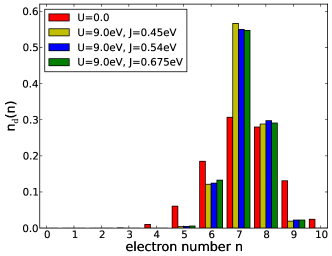
Figure 5: Local charge distribution of iron atoms $n_{d}(n)$ for $U=0$ (LDA limit) and $U=9\,{\rm eV}$ and $J/U=0.05,0.06,0.075$ (Gutzwiller-DFT) for optimal lattice parameters.

The average $3d$-electron density $n_{d}$ and the magnetization $m$ do not change much as a function of $(U,J)$. However, this does not imply that correlations are small in iron. In order to display the correlated nature of the ground state, we study some local properties.

First, we discuss the local charge distribution $n_{d}(n)$ which gives the probability to find $n$ electrons in the $3d$ shell on an iron atom. Figure 5 shows $n_{d}(n)$ from Gutzwiller-DFT in the LDA limit, $U=0$, and for $U=9\,{\rm eV}$ and $J/U=0.05,0.06,0.075$. For $U=0$ we find quite a broad distribution $n_{d}(n)$ with significant values for $n_{d}(n)$ for $4\leq n\leq 10$. For $U=9.0\,{\rm eV}$ and $J/U=0.05,0.06,0.075$, only configurations with $n=6,7,8$ electrons in the $3d$ shell have a substantial weight. This does not come as a surprise because the Gutzwiller correlator suppresses the occupation of local configurations that are energetically unfavorable. This behavior was also observed in previous studies. Schickling2011 ; Schickling2012

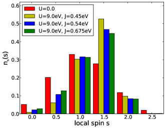
Figure 6: Local spin distribution of iron atoms $n_{s}(s)$ for $U=0$ (LDA limit) and $U=9\,{\rm eV}$ and $J/U=0.05,0.06,0.075$ (Gutzwiller-DFT) for optimal lattice parameters.

More revealing is the local spin distribution function $n_{s}(s)$ shown in Fig. 6 where $n_{s}(s)$ gives the probability to find the local spin quantum number $s$ on an iron atom. From $n_{s}(s)$ we can calculate the expectation value for the local spin as

$$\langle\hat{{\mathbf{S}}}_{i}^{2}\rangle=\sum_{s}n_{s}(s)s(s+1)\equiv S_{m}(S_{m}+1)\;.$$ (17)

Here, $S_{m}$ defines our average spin per atom. Figure 6 shows that the local spin distribution is fairly broad for $U=0$. Since $n_{d}=5$ is finite for $U=0$, the local spin distribution has a finite weight even for $s=5/2$. For $U=9\,{\rm eV}$, the local configurations $3d^{7}$ and $3d^{8}$ dominate, see Fig. 5. Therefore, applying Hund’s first rule, we expect to find peaks in the local spin distribution $n_{s}(s)$ at $s=3/2$ and $s=1$ which is indeed seen in Fig. 6. Concomitantly, the average spin per atom is a bit larger for $U=9\,{\rm eV}$, $S_{m}=1.3$ for $J/U=0.06$, than for $U=0$, $S_{m}^{\rm LDA}=1.23$.

In contrast to Hund’s first rule, $S_{m}(J)$ decreases as a function of the Hund’s-rule coupling $J$. This is seen from Fig. 6 which shows that the weight of configurations with spin $s=0,1/2$ increases at the expense of configurations with spin $s=3/2$. Therefore, both the overall magnetization $m$ and the local spin $S_{m}$ decrease as a function of the Hund’s-rule coupling. This seems to contradict Hund’s first rule which states that, in an atom, a larger $J$ stabilizes configurations with a larger spin. Apparently, the solution to this problem must be related to the fact that we are investigating a metal in which band-magnetism dominates.

In table 1 we list the values for several quantities for $J/U=0.05$, $J/U=0.06$ and $J/U=0.075$ at fixed $U=9.0\,{\rm eV}$ and fixed lattice parameter $a=5.39a_{\rm B}$. The data redisplay the behavior seen in figures 2 and 6: when we increase $J/U$, the magnetization $m$ decreases. Note, however, that upon an increase of $J/U$, the electronic correlations actually increase, too, as can be seen from the bandwidth reduction factors $(q^{2})$. The itineracy of the electrons becomes progressively worse when the weight of local configurations is redistributed by the Gutzwiller correlator for increasing $J/U$. The effect of the Hund’s-rule coupling on the bandwidth reduction is fairly pronounced. The $(q^{2})$-factors decrease by $\Delta(q^{2})\approx 0.2$ when we vary $U$ from zero to $U=9.0\,{\rm eV}$ but they change by as much as $\Delta(q^{2})\approx 0.1$ for the majority spin species when we go from $J/U=0.05$ to $J/U=0.075$ at $U=9\,{\rm eV}$. Apparently, it is favorable for the kinetic energy to flip majority spins back to minority spins, i.e., there is a tendency to reduce the magnetization as a function of $J/U$. As seen from table 1, the partial occupancy $n_{e_{g}}$ of the $e_{g}$-levels remains almost unchanged, and the reduction of the magnetization from $m=2.49\mu_{\rm B}$ at $J/U=0.05$ to $m=2.05\mu_{\rm B}$ at $J/U=0.075$ is generated by flipping majority-spin $t_{2g}$-electrons.

Table 1: Magnetization $m$, bandwidth reduction factors $(q_{e_{g}})^{2}$ and $(q_{t_{2g}})^{2}$ for $3d(e_{g})$ and $3d(t_{2g})$ electrons, respectively (resolved for majority spins and minority spins), kinetic energy $E_{\rm kin}$ per atom, and interaction energy $E_{\rm int}$ per atom; Gutzwiller-DFT data for $U=9.0\,{\rm eV}$ for $J/U=0.05,0.06,0.075$. The lattice parameter is fixed at $a=5.39a_{\rm B}$.

	A$J/U=0.05$	$J/U=0.06$	$J/U=0.075$
$m/\mu_{\rm B}$	2.49	2.24	2.05A
$(q_{e_{g}})^{2}$	0.794, 0.799	0.748, 0.799	0.712, 0.795
$(q_{t_{2g}})^{2}$	0.790, 0.783	0.746, 0.779	0.718, 0.770
$n_{e_{g}}$	0.985, 0.350	0.985, 0.341	0.985, 0.332
$n_{t_{2g}}$	0.970, 0.546	0.925, 0.594	0.887, 0.632
$E_{\rm kin}$/eV	94.82	94.90	95.05
$E_{\rm int}$/eV	1.68	1.48	1.16

The Hund’s-rule coupling $J$ changes the weight of iso-electronic local configurations with different spin. Apparently, this level splitting impedes the average electron transfer between atoms much more than the elimination of charge states with $n=4,5,9,10$ by the Hubbard interaction $U$. The loss in kinetic energy by this ‘configurational hopping blockade’ cannot be compensated fully by a gain in local interaction energy that is at most of the order of $\Delta E_{J}=(J_{1}S_{m,1}-J_{2}S_{m,2})$ with $\Delta E_{J}\approx 0.2\,{\rm eV}$ per atom in our example. Instead, the system prefers to re-gain kinetic energy by reducing the magnetization at the price of loosing exchange energy; recall that in a band magnet the loss in kinetic energy is compensated by the gain in exchange energy. Since all quantities are determined self-consistently in Gutzwiller-DFT, the kinetic energy, the exchange energy, and the gain in Hund’s-rule energy must be newly balanced to re-adjust $m$ when we change $J/U$ for fixed $U$. Apparently, in band magnets we observe a intricate interplay between atomic and bandstructure physics.

IV Bandstructure

IV.1 Bandwidth renormalization

We begin with a comparison of the quasi-particle bands from DFT(LDA), DFT(GGA) and Gutzwiller-DFT with $U=9\,{\rm eV}$ and $J/U=0.06$ for ferromagnetic bcc iron at ambient pressure ($a=5.39a_{\rm B}$). Moreover, we compare bands from DFT(LDA) and Gutzwiller-DFT for non-magnetic hcp iron with lattice parameter $a_{\rm hcp}=4.60a_{\rm B}$ and $(c/a)_{\rm hcp}=1.60$; the results change marginally when we use the ideal ratio $(c/a)_{\rm ideal}=\sqrt{8/3}=1.63$.

In order to obtain smooth band plots and to include the effects of the spin-orbit coupling on the bandstructure perturbatively, see Sect. IV.2.1, we introduced a further post-processing step. The Gutzwiller Kohn-Sham quasi-particles were used to generate maximally-localized Wannier functions using Wannier90, Mostofi2008685 from which we constructed a tight-binding model to calculate the band structure at arbitrary ${\bf k}$-points. These Wannier functions are used only for plotting purposes, and are unrelated to those chosen to perform the self-consistent calculations.

We checked that the tight-binding dispersion relation agrees with the calculated energy levels from Quantum ESPRESSO for our selected independent ${\bf k}$-points in the Brillouin zone. The small wiggles in the $4s$-bands close to the $\Gamma$ point seen in Fig. 7 are a result of the tight-binding fit. We disregard the problem because this does not influence the $3d$-bands close to the Fermi energy and has no effect on the total energy which is calculated using the original quasi-particles.

IV.1.1 Ferromagnetic bcc iron

In Fig. 7 we compare the bandstructure for ferromagnetic bcc iron from DFT(LDA) and from Gutzwiller-DFT for $U=9.0\,{\rm eV}$ and $J=0.54\,{\rm eV}$. Both calculations are performed at the optimal lattice parameter, $a^{\rm LDA}=5.21a_{\rm B}$ and $a^{\rm GDFT}=5.39a_{\rm B}$. Fig. 7 shows the common characteristics of correlation-induced effects on energy bands. First, the uncorrelated, $4sp$-type parts of the quasi-particle bands deep below the Fermi energy do not differ much, e.g., the lowest $4sp$-type majority bands are at $\Gamma_{{\rm low},\uparrow}^{\rm LDA}=9.0\,{\rm eV}$ and $\Gamma_{{\rm low},\uparrow}^{\text{G-DFT}}=8.57\,{\rm eV}$ below the Fermi energy $E_{\rm F}=0$. Minor deviations are related to slightly different lattice parameters and $3d$-electron numbers $\overline{n}_{d}$ in DFT(LDA) and Gutzwiller-DFT.

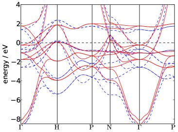
Figure 7: Comparison between DFT(LDA) bands (blue, dashed lines) for $a^{\rm LDA}=5.21a_{\rm B}$ and bands from Gutzwiller-DFT (red, full lines) for the optimal atomic parameters $U=9.0\,{\rm eV}$ and $J=0.54\,{\rm eV}$ and $a=5.39a_{\rm B}$ for ferromagnetic bcc iron. For clarity, we do not discriminate between majority and minority spin bands. The Fermi energy is at $E_{\rm F}=0$ (dashed black horizontal line).

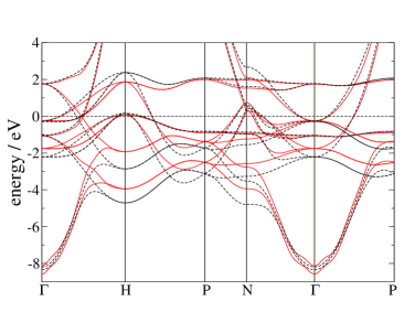
Figure 8: Comparison between DFT(GGA) bands (black, dashed lines) for $a_{\rm GGA}=5.39a_{\rm B}$ and bands from Gutzwiller-DFT (red, full lines) for the optimal atomic parameters $U=9.0\,{\rm eV}$ and $J=0.54\,{\rm eV}$ and $a=5.39a_{\rm B}$ for ferromagnetic bcc iron. For clarity, we do not discriminate between majority and minority spin bands. The Fermi energy is at $E_{\rm F}=0$ (dashed horizontal line).

Second, the Gutzwiller-correlated $3d$-type parts of the quasi-particle bands close to the Fermi energy are shifted with respect to the DFT(LDA) bands, and the bandwidths of the correlated bands are reduced by factors proportional to $(q_{t_{2g}})^{2}$ and $(q_{e_{g}})^{2}$ for the $3d$-$t_{2g}$ and $3d$-$e_{g}$ majority and minority bands. Note that, due to the hybridization of the quasi-particles, a meaningful symmetry character can only be assigned to the bands at high-symmetry points in the Brillouin zone.

The bandwidth reduction in iron is not as strong as in nickel. Nevertheless, for selected symmetry points, the discrepancies between the quasi-particle bands from DFT(LDA) and Gutzwiller-DFT are quite large. For example, at the H-point in the Brillouin zone we find a bandwidth reduction for the majority band by 36%, from $H_{{\rm low},\uparrow}^{\rm LDA}=5.38\,{\rm eV}$ down to $H_{{\rm low},\uparrow}^{\text{G-DFT}}=3.94\,{\rm eV}$, in good agreement with experiment, $H_{{\rm low},\uparrow}=3.8\,{\rm eV}$. PhysRevB.29.2986 Likewise, at the N-point in the Brillouin zone there is a majority spin band at $N_{{\rm low},\uparrow}=4.5\,{\rm eV}$ below the Fermi energy in experiment, PhysRevB.29.2986 in comparison with $N_{{\rm low},\uparrow}^{\rm LDA}=5.47\,{\rm eV}$ in DFT(LDA) and $N_{{\rm low},\uparrow}^{\text{G-DFT}}=3.90\,{\rm eV}$ in Gutzwiller-DFT. At the $\Gamma$-point the bandwidth reduction is only about 10% for bands close to the Fermi edge. In addition, the bandwidth renormalization at the $\Gamma$-point is overlaid with a bandshift of about $0.4\,{\rm eV}$.

For completeness, we show the bandstructure for ferromagnetic bcc iron from Gutzwiller-DFT for $U=9.0\,{\rm eV}$ and $J=0.54\,{\rm eV}$ in comparison with those from (scalar relativistic) DFT(GGA) calculations in Fig. 8. The two band structures differ less than in Fig. 7 because our DFT(GGA) provides the same equilibrium lattice parameter as used in Gutzwiller-DFT, $a_{\rm GGA}=5.39a_{\rm B}$. The bandwidth of the $3d$-electrons from the DFT(LDA) is calculated for $a_{\rm LDA}=5.21a_{\rm B}$ so that the $3d$-orbitals have a larger overlap in DFT(LDA) than in DFT(GGA), and the $3d$ bandwidth is larger in LDA than in GGA. Nevertheless, the correlations in the Gutzwiller approach lead to an additional bandwidth reduction of the $d$ bands across the Brillouin zone.

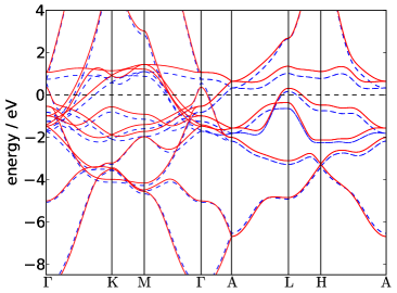
Figure 9: Comparison between DFT(LDA) bands (blue, dashed lines) and bands from Gutzwiller-DFT (red, full lines) for the atomic parameters $U=9.0\,{\rm eV}$ and $J=0.54\,{\rm eV}$ for paramagnetic hcp iron at $a=4.60a_{\rm B}$ and $c/a=1.60$. The Fermi energy is at $E_{\rm F}=0$ (dashed black horizontal line).

IV.1.2 Non-magnetic hcp iron

In Fig. 9 we compare the bandstructure for non-magnetic hcp iron from DFT(LDA) and from Gutzwiller-DFT for $U=9.0\,{\rm eV}$ and $J=0.54\,{\rm eV}$. Both calculations are performed at the lattice parameter $a=4.60a_{\rm B}$ and $c/a=1.60$ so that the unit-cell volume is $v_{0}=\sqrt{3}/2(a^{2}/2)c=67.4a_{\rm B}^{3}$. The partial densities are almost identical, $\overline{n}_{d}=7.3$.

As for ferromagnetic bcc iron, the uncorrelated, $4sp$-type parts of the quasi-particle bands deep below or high above the Fermi energy do not differ much. Again, the Gutzwiller-correlated $3d$-type parts of the quasi-particle bands close to the Fermi energy are shifted with respect to the DFT(LDA) bands, and the bandwidths of the correlated bands are reduced. The Fermi-liquid properties (Fermi surface topology, wavevectors, velocities) differ only quantitatively.

Table 2: Comparison of Fermi wavenumbers and velocities for various Fermi sheets between fully relativistic DFT(GGA), LDA+Gutzwiller for $U=9.0\,{\rm eV}$, $J=0.54\,{\rm eV}$, and $a=5.39a_{\rm B}$, and ARPES results. PhysRevB.72.155115 FS: Fermi sheet; $k_{\rm F}$: Fermi wavenumber; $v_{\rm F}=v/\hbar=\hbar k_{\rm F}/m$: Fermi velocity.

Direction	Spin	FS	$k_{\rm F}$ GGA $(\hbox{\AA}^{-1})$	$k_{\rm F}$ LDA+G $(\hbox{\AA}^{-1})$	$k_{\rm F}$ ARPES $(\hbox{\AA}^{-1})$	Slope $v_{\rm D}$ GGA $({\rm eV}\hbox{\AA})$	Slope $v_{\rm G}$ LDA+G $({\rm eV}\hbox{\AA})$	Slope $v_{\rm R}$ ARPES $({\rm eV}\hbox{\AA})$	Mass Ratio $v_{\rm D}/v_{\rm R}$	Mass Ratio $v_{\rm G}/v_{\rm R}$
$\Gamma$–P	Min.	VI	0.31	0.33	0.32	1.66	1.38	0.88	1.9	1.6
	Maj.	I	0.95	0.94	0.97	4.74	3.86	1.40	3.4	2.8
$\Gamma$–H	Min.	VI	0.47	0.49	0.46	1.08	0.83	0.72	1.5	1.2
	Maj.	I	1.09	1.10	1.08	2.36	3.35	1.12	2.1	3.0
		II	1.94	1.93	1.70	0.64	0.58	0.67	1.0	0.9
$\Gamma$–N	Min.	VI	0.33	0.35	0.36	1.52	1.25	0.80	1.9	1.6
	Maj.	I	1.21	1.21	1.22	1.89	1.53	1.16	1.6	1.3
H–P	Min.	V	0.65	0.64	0.68	4.82	4.16	1.79	2.7	2.3

IV.2 Comparison with ARPES measurements

IV.2.1 Inclusion of spin-orbit coupling

As effective parameter for the spin-orbit interaction we choose $\zeta=0.06\,{\rm eV}$, in agreement with previous studies. PhysRevB.11.287 ; PhysRevLett.92.037204 The small value permits a perturbative treatment of the spin-orbit coupling. In effect, it leads to negligibly small changes in the bandstructures but for avoided crossings of majority and minority bands where it induces bandgaps of the order of $\zeta$. Since some of the avoided crossings are energetically close to the Fermi energy, the spin-orbit interaction has some noticeable effect on the positions of the Fermi points and the Fermi velocities.

For our perturbative treatment, we start from the majority and minority bands as calculated from Gutzwiller-DFT for ($U=9.0\,{\rm eV}$, $J=0.54\,{\rm eV}$) at $a=5.39a_{\rm B}$ and use the program Wannier90 Mostofi2008685 to derive a tight-binding Hamilton operator. Then, the two block-diagonal parts of the Hamiltonian for majority and minority bands are coupled by the spin-orbit interaction. We obtain the bandstructure with spin-orbit coupling from the diagonalization of this effective Hamilton matrix. For larger values of $\zeta$, a fully self-consistent treatment of the spin-orbit interaction is necessary that requires the formulation of a relativistic Gutzwiller-DFT.

IV.2.2 Quasi-particle bands close to the Fermi energy

Figures 10 to 13 show an overlay of ARPES data from Schäfer et al. PhysRevB.72.155115 with the results of our perturbative spin-orbit calculation based on the Gutzwiller-DFT. A quantitative comparison between theory and experiment is given in table 2 where we list the Fermi wavenumbers and velocities for various directions and Fermi sheets LDA+Gutzwiller, and ARPES. PhysRevB.72.155115 For completeness, we also include in the table values from our fully relativistic GGA calculations, see Sect. II.3 for details.

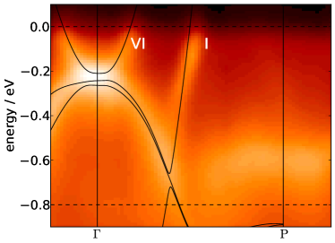
Figure 10: Overlay of quasi-particle bands from LDA+Gutzwiller for $U=9.0\,{\rm eV}$, $J=0.54\,{\rm eV}$, and lattice parameter $a=5.39a_{\rm B}$ with ARPES data along the $\Gamma$–P direction. PhysRevB.72.155115

We begin our discussion with the $\Gamma$–P high symmetry line in the Brillouin zone. From Fig. 10 we see that, close to the $\Gamma$-point, we observe a very good agreement between LDA+Gutzwiller and experimental data for the Fermi sheet VI. Moreover, the Fermi wavenumbers and the velocities agree very well, as seen from table 2. Our LDA+Gutzwiller improves the theoretical values for the Fermi velocity. The mass ratio between theory and experiment reduces from $v_{\rm D}/v_{\rm R}=1.9$ in DFT(GGA) to $v_{\rm G}/v_{\rm R}=1.6$ in LDA+Gutzwiller. Note that the mass ratio is unity for a perfect agreement between theory and experiment, and it is larger than unity when the theoretical mass is smaller than measured value, $v/v_{\rm R}=m_{\rm R}/m$.

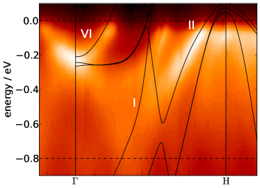
Figure 11: Overlay of quasi-particle bands from LDA+Gutzwiller for $U=9.0\,{\rm eV}$, $J=0.54\,{\rm eV}$, and lattice parameter $a=5.39a_{\rm B}$ with ARPES data along the $\Gamma$–H direction. PhysRevB.72.155115

The largest discrepancies between experiment and LDA+Gutzwiller theory are seen at and around the P-point. The LDA+Gutzwiller bands are about $0.3\,{\rm eV}$ below the ARPES bands, and the discrepancy in LDA+ Gutzwiller is actually worse than in LDA(GGA). We do not have an explanation for this deviation.

Half way on the line $\Gamma$–P there is the Fermi sheet I. For this band, the values for the Fermi wavenumbers from DFT(GGA) and LDA+Gutzwiller are very close to the experimental value but the Fermi velocities deviate considerably, even though LDA+Gutzwiller has a slightly better mass ratio, $v_{\rm G}/v_{\rm R}=2.8$ versus $v_{\rm D}/v_{\rm R}=3.4$.

In Fig. 11 we plot the data overlay along the high-symmetry line $\Gamma$–H. As discussed before, the agreement of the quasi-particle bands, wavenumbers and velocities of Fermi sheet VI close to the $\Gamma$-point is very good. The same holds true for the Fermi sheet II close to the H-point.

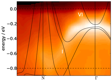
Figure 12: Overlay of quasi-particle bands from LDA+Gutzwiller for $U=9.0\,{\rm eV}$, $J=0.54\,{\rm eV}$, and lattice parameter $a=5.39a_{\rm B}$ with ARPES data along the N–$\Gamma$ direction. PhysRevB.72.155115

For the majority Fermi sheet I half way between the points $\Gamma$ and H we find a large mass ratio as in LDA(GGA), $v_{\rm G}/v_{\rm R}=3.0$ versus $v_{\rm D}/v_{\rm R}=2.1$. Note, however, that several bands meet at the Fermi energy with the same Fermi wavenumber, and the spin-orbit coupling leads to a splitting of bands. Therefore, it is difficult to determine the Fermi velocity due to the sequence of crossings. This region around the Fermi energy is not very suitable for a meaningful comparison between theory and experiment.

In Fig. 12 we plot the data overlay along the high-symmetry line N–$\Gamma$. In experiment, the intensity along this direction is suppressed close to the point N due to matrix-element effects. However, we reproduce a crossing of the Fermi energy close to the N-point and the slope of the bands agree quite well.

For the minority band VI close to the $\Gamma$-point we find a mass ratio of $v_{\rm G}/v_{\rm R}=1.6$, versus $v_{\rm D}/v_{\rm R}=1.9$ in DFT(GGA). For the majority band I half way between $\Gamma$ and N we find a mass ratio of $v_{\rm G}/v_{\rm R}=1.3$, versus $v_{\rm D}/v_{\rm R}=1.6$ in DFT(GGA). In both cases, we find a slight improvement over the DFT(GGA) results. Half way between the points N and $\Gamma$, it seems as if the LDA+Gutzwiller bands at energies of about $-0.5\,\mathrm{eV}$ do not agree very well with the ARPES bands but better experimental data are needed for a definitive statement.

Lastly, we take a look at the direction H–P in Fig. 13. As already seen from the other plots, the agreement at and around the point H is quite good while the comparison at point P reveals some discrepancies between theory and experiment. In addition, the ARPES data show some distinct Fermi level crossing half way between H and P. The LDA+Gutzwiller approach yields a Fermi wavenumber for this crossing that deviates slightly from experiment with a mass ratio $v_{\rm G}/v_{\rm R}=2.3$ versus $v_{\rm D}/v_{\rm R}=2.7$ in DFT(GGA).

Depending on the Fermi wavevector, the quasi-particle mass in Gutzwiller-DFT is some 20% larger than in DFT(GGA). A similar mass enhancement is observed in DFT(DMFT) calculations. PhysRevB.90.155120 ; PhysRevLett.103.267203 However, as seen from table 2, the mass ratio between theory and experiment is consistently larger than unity, $v_{\rm G}/v_{\rm R}=m_{\rm R}/m_{\rm G}>1$, and strongly depends on the Fermi wavevector. The correlation-induced mass enhancement alone cannot account for the large mass renormalization as seen in experiment. The resolution of this discrepancy remains one of the incompletely understood problems for iron and other magnetic materials.

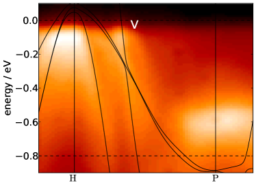
Figure 13: Overlay of quasi-particle bands from LDA+Gutzwiller for $U=9.0\,{\rm eV}$, $J=0.54\,{\rm eV}$, and lattice parameter $a=5.39a_{\rm B}$ with ARPES data along the H–P direction. PhysRevB.72.155115

V Conclusions

In this work, we used the Gutzwiller-DFT for a detailed study of the ground-state properties and the quasi-particle bandstructure of iron. We find that, for a Hubbard interaction of $U=9\,{\rm eV}$ and a Hund’s-rule coupling of $J=0.54\,{\rm eV}$, we reproduce the experimental lattice parameter and magnetization, and we obtain the bulk modulus of ferromagnetic bcc iron in very good agreement with experiment. Upon increasing pressure we qualitatively reproduce the transition to non-magnetic hcp iron.

We find that the ground-state magnetization sensitively depends on the Hund’s-rule coupling $J$. In contrast to physical intuition, an increase of $J$ leads to a decrease of the magnetization. For example, at $U=9\,{\rm eV}$, an increase from $J=0.45\,{\rm eV}$ to $J=0.68\,{\rm eV}$ decreases the magnetization from $m=2.5\mu_{\rm B}$ to $m=2.05\mu_{\rm B}$. The Hund’s-rule coupling generates a splitting of iso-electronic atomic levels, and the corresponding redistribution of local occupancies considerably impedes the electrons’ motion through the lattice (‘configurational hopping blockade’). In a band magnet, the delicate balance between the Hund’s-rule and exchange-energy gains against the corresponding losses in kinetic energy makes the magnetization sensitive to the Hund’s-rule coupling. Therefore, the absolute value of $J$ is much more decisive for physical quantities than the value of the Hubbard interaction. For the calculation of some physical quantities, a larger value of $J$ can be ‘traded in’ for a smaller $U$.

Gutzwiller-DFT renormalizes the quasi-particle bands as obtained from DFT(LDA). While the $4sp$-type parts are almost unchanged, the $3d$-bands are shifted and their width is reduced, in agreement with experiment. Shifts and renormalizations are also observed when we compare the Gutzwiller-DFT results with GGA calculations although the effects are quantitatively smaller.The applied double-counting corrections make sure that the average $3d$-electron density remains essentially the same, $\overline{n}_{d}\approx 7.2$. The agreement between the Gutzwiller quasi-particle bands with ARPES data is fairly good when we take spin-orbit effects into account perturbatively. In general, Gutzwiller-DFT agrees better with ARPES data than DFT, both in the LDA and GGA approximations.

Finally, we note that the optimal atomic parameters in the present Gutzwiller-DFT study on iron resemble those used by Deng et alii, Deng2008 ; Deng2009 but are sensibly higher than those used in a more recent Gutzwiller-DFT work by Borghi et al. PhysRevB.90.125102 who propound a $U$-parameter of $U_{\rm B}=2.5\,{\rm eV}$ for iron that is significantly smaller than our values. Part of the discrepancy is probably due to their different choice of energy window and basis set for the construction of the many-body model. However, there are also substantial differences already at the bare DFT(LDA) level ($U=J=0$); Borghi et al. use a localized orbital code (SIESTA) whose results deviate from other DFT codes for iron. Table III of Ref. [PhysRevB.90.125102, ] gives the lattice constant $a_{\rm Borghi}=2.83\,\hbox{\AA}=5.35a_{\rm B}$, while we find $a_{0}=5.2a_{\rm B}$, in agreement with earlier LDA-LAPW calculations. PhysRevLett.54.1852 Since the lattice constant monotonically increases as a function of $U$, see Fig. 1, it is not surprising that Borghi et al. require a smaller Hubbard interaction to reproduce the experimental lattice parameter $a=5.42a_{\rm B}$, and claim a different role of electronic correlations in iron.

Despite the improvements of Gutzwiller-DFT and DFT(DMFT) over standard DFT(LDA and GGA), the theoretical Fermi velocities are typically too large, i.e., the quasi-particle masses from theory are too low in comparison with experiment. This systematic discrepancy could have several reasons. First, it might be necessary to process the theoretical bandstructures further to mimic the excitation process in ARPES experiments. 1367-2630-12-1-013007 However, this approach could not explain why the systematic mass enhancement is also seen in de-Haas–van-Alphen measurements for iron and ferromagnetic nickel-compounds. JMMM-Lonzarich Therefore, it is more likely that the effective mass results from the interaction of the quasi-particles with low-energy magnetic excitations, i.e., magnetic polarons exist near the Fermi energy. PhysRevLett.92.097205 At present, however, the inclusion of long wave-length excitations is beyond the Gutzwiller-DFT.

Appendix A Atomic interactions and double counting

For the $3d$ shell of $e_{g}$ and $t_{2g}$ orbitals in transition metals the local Hamiltonian (2) reads ($\sigma=\uparrow,\downarrow$)

$$\hat{V}_{\rm loc}=\frac{1}{2}\sum_{c,\sigma}U(c,c)\hat{n}_{c,\sigma}\hat{n}_{c^{\prime},\bar{\sigma}}+\frac{1}{2}\!\!\sum_{\genfrac{}{}{0.0pt}{2}{c(\neq)c^{\prime}}{\sigma,\sigma^{\prime}}}\!\!\widetilde{U}_{\sigma,\sigma^{\prime}}(c,c^{\prime})\hat{n}_{c,\sigma}\hat{n}_{c^{\prime},\sigma^{\prime}}$$

$$+\frac{1}{2}\sum_{c(\neq)c^{\prime}}J(c,c^{\prime})\left(\hat{c}^{\dagger}_{c,\uparrow}\hat{c}^{\dagger}_{c,\downarrow}\hat{c}_{c^{\prime},\downarrow}\hat{c}_{c^{\prime},\uparrow}+{\rm h.c.}\right)$$

$$+\frac{1}{2}\sum_{c(\neq)c^{\prime};\sigma}J(c,c^{\prime})\hat{c}^{\dagger}_{c,\sigma}\hat{c}^{\dagger}_{c^{\prime},\bar{\sigma}}\hat{c}_{c,\bar{\sigma}}\hat{c}_{c^{\prime},\sigma}$$

$$+\bigg{[}\sum_{t;\sigma,\sigma^{\prime}}(T(t)-\delta_{\sigma,\sigma^{\prime}}A(t))\hat{n}_{t,\sigma}\hat{c}^{\dagger}_{u,\sigma^{\prime}}\hat{c}_{v,\sigma^{\prime}}$$

$$\hphantom{+\bigg{[}}+\sum_{t,\sigma}A(t)\left(\hat{c}^{\dagger}_{t,\sigma}\hat{c}^{\dagger}_{t,\bar{\sigma}}\hat{c}_{u,\bar{\sigma}}\hat{c}_{v,\sigma}+\hat{c}^{\dagger}_{t,\sigma}\hat{c}^{\dagger}_{u,\bar{\sigma}}\hat{c}_{t,\bar{\sigma}}\hat{c}_{v,\sigma}\right)$$

$$\hphantom{+\bigg{[}}+\sum_{\genfrac{}{}{0.0pt}{2}{t(\neq)t^{\prime}(\neq)t^{\prime\prime}}{e,\sigma,\sigma^{\prime}}}S(t,t^{\prime};t^{\prime\prime},e)\hat{c}^{\dagger}_{t,\sigma}\hat{c}^{\dagger}_{t^{\prime},\sigma^{\prime}}\hat{c}_{t^{\prime\prime},\sigma^{\prime}}\hat{c}_{e,\sigma}+{\rm h.c.}\bigg{]}\;.$$

(18)

Note that the factors $1/2$ in the first three lines have been erroneously missing in our previous publications [1367-2630-16-9-093034, ] and [Schickling2011, ]. Here, $\widetilde{U}_{\sigma,\sigma^{\prime}}(c,c^{\prime})=U(c,c^{\prime})-\delta_{\sigma,\sigma^{\prime}}J(c,c^{\prime})$, and we suppressed the site index ${\mathbf{R}}$. The index $c$ sums over all five $d$-orbitals while $t$ and $e$ are indices for the three $t_{2g}$ orbitals with symmetries $xy$, $xz$, and $yz$ and the two $e_{g}$ orbitals with symmetries $u=3z^{2}-r^{2}$ and $v=x^{2}-y^{2}$, respectively. Of all the parameters $U(c,c^{\prime})$, $J(c,c^{\prime})$, $A(t)$, $T(t)$, $S(t,t^{\prime};t^{\prime\prime},e)$ only ten are independent in cubic symmetry. 1367-2630-16-9-093034 ; Sugano1970 When we assume that all 3$d$-orbitals have the same radial wavefunction (‘spherical approximation’), all parameters are determined by, e.g., the three Racah parameters $A,B,C$. They are related to the Slater-Condon parameters via

$$A=F^{(0)}-\frac{F^{(4)}}{9}\;,\;B=\frac{1}{49}\Bigl{(}F^{(2)}-\frac{5}{9}F^{(4)}\Bigr{)}\;,\;C=\frac{5}{63}F^{(4)}\;,$$ (19)

or, inversely,

$$F^{(0)}=A+\frac{7}{5}C\quad,\quad F^{(2)}=49B+7C\quad,\quad F^{(4)}=\frac{63}{5}C\;.$$ (20)

Explicit expressions for the relations between the parameters in eq. (18) and the Racah parameters $A,B,C$ can be found in appendix C of Ref. [1367-2630-16-9-093034, ]. For comparison with other work, we introduce the Coulomb interaction between electrons in the same 3$d$-orbitals (intra-orbital Hubbard interaction),

$$U=A+4B+3C\;,$$ (21)

the average Coulomb interaction between electrons in different orbitals (inter-orbital Hubbard interaction),

$$U^{\prime}=\frac{1}{10}\sum_{c<c^{\prime}_{\displaystyle\vphantom{X}}}U(c,c^{\prime})=A-B+C\;,$$ (22)

and the average Hund’s-rule exchange interaction,

$$J=\frac{1}{10}\sum_{c<c^{\prime}}J(c,c^{\prime})=\frac{5}{2}B+C\;.$$ (23)

These three quantities are not independent but related by the symmetry relation $U^{\prime}=U-2J$. This means that by choosing two of these parameters (e.g., $U$ and $J$) the three Racah parameters, and therefore all the parameters in Eq. (18) are not uniquely defined. Hence, we use the additional relation $C/B=4$ which is a reasonable assumption for transition metals. Sugano1970 It corresponds to $F^{(2)}/F^{(4)}=55/36=1.53$, in agreement with the estimate $F^{(2)}/F^{(4)}\approx 1.60=8/5$ by de Groot et alii. PhysRevB.42.5459 For completeness, we give the dependencies of the Racah parameters on $U$ and $J$

$$A=U-\frac{32}{13}J\quad,\quad B=\frac{2}{13}J\quad,\quad C=\frac{8}{13}J\;.$$ (24)

In our previous study on nickel,1367-2630-16-9-093034 we have tested three different types of double-counting corrections that had been proposed in the literature. It turned out that only one of them leads to sensible results for nickel. As for nickel 1367-2630-16-9-093034 we employ the widely used functional PhysRevB.44.943 ; PhysRevB.52.R5467

$$V_{\rm dc}=\frac{\bar{U}}{2}\bar{n}(\bar{n}-1)-\frac{\bar{J}}{2}\sum_{\sigma}\bar{n}_{\sigma}(1-\bar{n}_{\sigma})\;.$$ (25)

For $3d$-electrons we have

$$F^{(0)}=\bar{U}=\frac{1}{5}\left(U+4U^{\prime}\right)\quad,\quad\bar{J}=\bar{U}-U^{\prime}+J\;,$$ (26)

and

$$\bar{n}_{\sigma}\equiv\sum_{c=1}^{N_{c}}C_{c,c;\sigma}^{\rm G}\quad,\quad\bar{n}\equiv\bar{n}_{\uparrow}+\bar{n}_{\downarrow}\;,$$ (27)

where $N_{c}$ is the number of correlated orbitals, in our case, $N_{c}=5$. Moreover,

$$C_{c,c;\sigma}^{\rm G}=\frac{\langle\Psi_{\rm G}|\hat{c}_{{\mathbf{R}},c,\sigma}^{+}\hat{c}_{{\mathbf{R}},c,\sigma}^{\vphantom{+}}|\Psi_{\rm G}\rangle}{\langle\Psi_{\rm G}|\Psi_{\rm G}\rangle}=\langle\psi_{0}|\hat{c}_{{\mathbf{R}},c,\sigma}^{+}\hat{c}_{{\mathbf{R}},c,\sigma}^{\vphantom{+}}|\psi_{0}\rangle$$ (28)

is the $\sigma$-electron density for the correlated $3d$ orbital $c$ in the Gutzwiller wavefunction. Note that the second equality only holds in the limit of infinite dimensions for our $e_{g}$-$t_{2g}$ orbital structure. 1367-2630-16-9-093034

References

- (1) C. S. Wang, B. M. Klein, and H. Krakauer, Phys. Rev. Lett. 54, 1852 (1985)
- (2) S. K. Bose, O. V. Dolgov, J. Kortus, O. Jepsen, and O. K. Andersen, Phys. Rev. B 67, 214518 (2003)
- (3) L. Stixrude, R. E. Cohen, and D. J. Singh, Phys. Rev. B 50, 6442 (1994)
- (4) M. Ekman, B. Sadigh, K. Einarsdotter, and P. Blaha, Phys. Rev. B 58, 5296 (1998)
- (5) J. P. Perdew, K. Burke, and M. Ernzerhof, Phys. Rev. Lett. 77, 3865 (1996)
- (6) G. Steinle-Neumann, L. Stixrude, and R. E. Cohen, Phys. Rev. B 60, 791 (1999)
- (7) G. Y. Guo and H. H. Wang, Chin. J. of Phys. 38, 949 (2000)
- (8) T. Schickling, J. Bünemann, F. Gebhard, and W. Weber, New Journal of Physics 16, 93034 (2014)
- (9) K. Glazyrin, L. V. Pourovskii, L. Dubrovinsky, O. Narygina, C. McCammon, B. Hewener, V. Schünemann, J. Wolny, K. Muffler, A. I. Chumakov, W. Crichton, M. Hanfland, V. B. Prakapenka, F. Tasnádi, M. Ekholm, M. Aichhorn, V. Vildosola, A. V. Ruban, M. I. Katsnelson, and I. A. Abrikosov, Phys. Rev. Lett. 110, 117206 (2013)
- (10) J. Hubbard, Proc. Royal Soc. A 276, 238 (1963)
- (11) M. C. Gutzwiller, Phys. Rev. Lett. 10, 159 (1963)
- (12) J. Hubbard, Proc. Royal Soc. A 277, 237 (1964)
- (13) M. C. Gutzwiller, Phys. Rev. 134, A923 (1964)
- (14) G. Kotliar, S. Y. Savrasov, K. Haule, V. S. Oudovenko, O. Parcollet, and C. A. Marianetti, Rev. Mod. Phys. 78, 865 (2006)
- (15) D. Vollhardt, Ann. Phys. 524, 1 (2012)
- (16) E. Gull, A. J. Millis, A. I. Lichtenstein, A. N. Rubtsov, M. Troyer, and P. Werner, Rev. Mod. Phys. 83, 349 (2011)
- (17) A. S. Belozerov and V. I. Anisimov, Journal of Physics: Condensed Matter 26, 375601 (2014)
- (18) L. V. Pourovskii, J. Mravlje, M. Ferrero, O. Parcollet, and I. A. Abrikosov, Phys. Rev. B 90, 155120 (2014)
- (19) K. M. Ho, J. Schmalian, and C. Z. Wang, Phys. Rev. B 77, 073101 (2008)
- (20) X. Deng, X. Dai, and Z. Fang, EPL (Europhysics Letters) 83, 37008 (2008)
- (21) X. Y. Deng, L. Wang, X. Dai, and Z. Fang, Phys. Rev. B 79, 075114 (2009)
- (22) G.-T. Wang, X. Dai, and Z. Fang, Phys. Rev. Lett. 101, 066403 (2008)
- (23) G. T. Wang, Y. Qian, G. Xu, X. Dai, and Z. Fang, Phys. Rev. Lett. 104, 047002 (2010)
- (24) H. Weng, G. Xu, H. Zhang, S.-C. Zhang, X. Dai, and Z. Fang, Phys. Rev. B 84, 060408 (2011)
- (25) Y. X. Yao, J. Schmalian, C. Z. Wang, K. M. Ho, and G. Kotliar, Phys. Rev. B 84, 245112 (2011)
- (26) M.-F. Tian, X. Deng, Z. Fang, and X. Dai, Phys. Rev. B 84, 205124 (2011)
- (27) N. Lanatà, H. U. R. Strand, X. Dai, and B. Hellsing, Phys. Rev. B 85, 035133 (2012)
- (28) N. Lanatà, H. U. R. Strand, G. Giovannetti, B. Hellsing, L. de’ Medici, and M. Capone, Phys. Rev. B 87, 045122 (2013)
- (29) N. Lanatà, Y.-X. Yao, C.-Z. Wang, K.-M. Ho, J. Schmalian, K. Haule, and G. Kotliar, Phys. Rev. Lett. 111, 196801 (2013)
- (30) N. Lanatà, Y.-X. Yao, C.-Z. Wang, K.-M. Ho, and G. Kotliar, Phys. Rev. B 90, 161104 (2014)
- (31) R. Dong, X. Wan, X. Dai, and S. Y. Savrasov, Phys. Rev. B 89, 165122 (2014)
- (32) N. Lanatà, Y. Yao, C.-Z. Wang, K.-M. Ho, and G. Kotliar, Phys. Rev. X 5, 011008 (2015)
- (33) G. Borghi, M. Fabrizio, and E. Tosatti, Phys. Rev. B 90, 125102 (2014)
- (34) T. Schickling, F. Gebhard, J. Bünemann, L. Boeri, O. K. Andersen, and W. Weber, Phys. Rev. Lett. 108, 036406 (2012)
- (35) J. Schäfer, M. Hoinkis, E. Rotenberg, P. Blaha, and R. Claessen, Phys. Rev. B 72, 155115 (2005)
- (36) J. Bünemann, F. Gebhard, T. Schickling, and W. Weber, physica status solidi (b) 249, 1282 (2012)
- (37) V. I. Anisimov, J. Zaanen, and O. K. Andersen, Phys. Rev. B 44, 943 (1991)
- (38) A. I. Liechtenstein, V. I. Anisimov, and J. Zaanen, Phys. Rev. B 52, R5467 (1995)
- (39) P. Giannozzi, S. Baroni, N. Bonini, M. Calandra, R. Car, C. Cavazzoni, D. Ceresoli, G. L. Chiarotti, M. Cococcioni, I. Dabo, A. D. Corso, S. de Gironcoli, S. Fabris, G. Fratesi, R. Gebauer, U. Gerstmann, C. Gougoussis, A. Kokalj, M. Lazzeri, L. Martin-Samos, N. Marzari, F. Mauri, R. Mazzarello, S. Paolini, A. Pasquarello, L. Paulatto, C. Sbraccia, S. Scandolo, G. Sclauzero, A. P. Seitsonen, A. Smogunov, P. Umari, and R. M. Wentzcovitch, Journal of Physics: Condensed Matter 21, 395502 (2009)
- (40) See Supplemental Material at [URL will be inserted by publisher] for the implementation of the Gutzwiller-DFT in Quantum ESPRESSO.
- (41) H. L. Zhang, S. Lu, M. P. J. Punkkinen, Q.-M. Hu, B. Johansson, and L. Vitos, Phys. Rev. B 82, 132409 (2010)
- (42) H. Danan, A. Herr, and A. J. P. Meyer, J. Appl. Phys. 39, 669 (1968)
- (43) A. A. Katanin, A. I. Poteryaev, A. V. Efremov, A. O. Shorikov, S. L. Skornyakov, M. A. Korotin, and V. I. Anisimov, Phys. Rev. B 81, 045117 (2010)
- (44) I. Leonov, A. I. Poteryaev, V. I. Anisimov, and D. Vollhardt, Phys. Rev. Lett. 106, 106405 (2011)
- (45) I. Leonov, A. I. Poteryaev, Y. N. Gornostyrev, A. I. Lichtenstein, M. I. Katsnelson, V. I. Anisimov, and D. Vollhardt, Scientific Reports 4, 5585 (2014)
- (46) A. I. Lichtenstein, M. I. Katsnelson, and G. Kotliar, Phys. Rev. Lett. 87, 067205 (2001)
- (47) T. Miyake, F. Aryasetiawan, and M. Imada, Phys. Rev. B 80, 155134 (2009)
- (48) T. Schickling, F. Gebhard, and J. Bünemann, Phys. Rev. Lett. 106, 146402 (2011)
- (49) F. Aryasetiawan, K. Karlsson, O. Jepsen, and U. Schönberger, Phys. Rev. B 74, 125106 (2006)
- (50) F. M. F. de Groot, J. C. Fuggle, B. T. Thole, and G. A. Sawatzky, Phys. Rev. B 42, 5459 (1990)
- (51) J. Sánchez-Barriga, J. Fink, V. Boni, I. Di Marco, J. Braun, J. Minár, A. Varykhalov, O. Rader, V. Bellini, F. Manghi, H. Ebert, M. I. Katsnelson, A. I. Lichtenstein, O. Eriksson, W. Eberhardt, and H. A. Dürr, Phys. Rev. Lett. 103, 267203 (2009)
- (52) A. P. Jephcoat, H. K. Mao, and P. M. Bell, Journal of Geophysical Research: Solid Earth 91, 4677 (1986), ISSN 2156-2202
- (53) O. K. Andersen, J. Madsen, U. K. Poulsen, O. Jepsen, and J. Kollar, Physica B 86–88, 249 (1977)
- (54) D. Bancroft, E. L. Peterson, and S. Minshall, J. Appl. Phys. 27, 291 (1956)
- (55) V. Iota, J.-H. P. Klepeis, C.-S. Yoo, J. Lang, D. Hasekl, and G. Srajer, Appl. Phys. Lett. 90, 042505 (2007)
- (56) A. A. Mostofi, J. R. Yates, Y.-S. Lee, I. Souza, D. Vanderbilt, and N. Marzari, Computer Physics Communications 178, 685 (2008)
- (57) A. M. Turner, A. W. Donoho, and J. L. Erskine, Phys. Rev. B 29, 2986 (1984)
- (58) M. Singh, C. S. Wang, and J. Callaway, Phys. Rev. B 11, 287 (1975)
- (59) Y. Yao, L. Kleinman, A. H. MacDonald, J. Sinova, T. Jungwirth, D.-S. Wang, E. Wang, and Q. Niu, Phys. Rev. Lett. 92, 037204 (2004)
- (60) A. L. Walter, J. D. Riley, and O. Rader, New Journal of Physics 12, 013007 (2010)
- (61) G. G. Lonzarich, Journal of Magnetism and Magnetic Materials 45, 43 (1984)
- (62) J. Schäfer, D. Schrupp, E. Rotenberg, K. Rossnagel, H. Koh, P. Blaha, and R. Claessen, Phys. Rev. Lett. 92, 097205 (2004)
- (63) J. D. Hunter, Computing in Science & Engineering 9, 90 (2007)
- (64) S. Sugano, Y. Tanabe, and H. Kamimura, Multiplets of Transition-Metal Ions in Crystals (Academic Press, New York, 1970)