Finite Temperature Quantum Effects on Confined Charges

Abstract

A quantum system of $N$ Coulomb charges confined within a harmonic trap is considered over a wide range of densities and temperatures. A recently described construction of an equivalent classical system is applied in order to exploit the rather complete classical description of harmonic confinement via liquid state theory. Here, the effects of quantum mechanics on that representation are described with attention focused on the origin and nature of shell structure. The analysis extends from the classical strong Coulomb coupling conditions of dusty plasmas to the opposite limit of low temperatures and large densities characteristic of ”warm, dense matter”.

I Introduction and Motivation

Coulomb correlations have been the focus of intense study for more than fifty years. Weak coupling conditions, both classical and quantum, are now well understood. The more interesting and difficult conditions of strong Coulomb coupling are well understood only in the limiting cases of zero temperature (electrons) and high temperatures (classical ions). Renewed interest in the intermediate cross-over domain between quantum and classical limits at arbitrary coupling has followed from new experimental studies of “warm, dense matter” WDM , new theoretical approaches PDW ; DuftyDutta ; DuttaDufty ; DD13 ; Liu14 , and new path integral Monte Carlo simulations Brown . The objective here is to explore this domain of finite temperatures for the case of charges in a harmonic trap under conditions where confinement, strong coupling, and quantum effects can appear together. Of particular interest is the role of these conditions in the formation and characterization of shell structure.

The approach here is to exploit classical many-body methods that treat Coulomb coupling effectively, such as classical density functional theory Lutsko , liquid state theory Hansen , or molecular dynamics simulation MD . It is necessary first to embed relevant quantum effects in a classical statistical mechanics. This has been shown to be an accurate and practical idea recently by Perrot and Dharma-wardana PDW using liquid state theory, by introducing a pair potential modified to include exchange and diffraction effects and an effective temperature to admit a finite kinetic energy at zero temperature. This approach was formalized for a more precise context by two of the current authors DuftyDutta , and a preliminary application to confined charges was described DuttaDufty . This effective liquid state approach has proved accurate for the thermodynamics and structure of the uniform electron gas over a wide range of densities and temperatures DD13 ; Liu14 . It is particularly useful for the problem posed here since there is now a rather complete study of the classical “Coulomb balls” via liquid state theory and classical Monte Carlo simulations Wrighton . Once the effective quantum potentials and thermodynamic parameters are specified, these same methods can be applied directly to the questions of quantum effects on shell formation. That is the objective of the work presented here.

At equilibrium the harmonically confined system is specified by the average number of particles in the trap, $\overline{N}$, the temperature, $T$, and the strength of the confining potential. The latter determines the volume of the system (see below) so that ultimately the harmonic potential parameters can be expressed in terms of the density and temperature. In the classical limit, all density and temperature dependence of dimensionless quantities occurs only through the classical Coulomb coupling constant, $\Gamma\equiv q^{2}/(r_{0}k_{B}T)$, where $q$ is the charge and $r_{0}$ is the Wigner-Seitz length related to the average global density $\overline{n}$ by $r_{0}=(4\pi\overline{n}/3)^{-1/3}$. It is a measure of the Coulomb energy for a pair of charges relative to the average kinetic energy per particle, $q^{2}/k_{B}Tr=\Gamma/r^{\ast}$ where $r^{\ast}=r/r_{0}$. In the classical case the primary results are that shell structure (peaks in the radial density profile) appear only at sufficiently strong coupling ($\Gamma\gtrsim 10$) and sharpen as the coupling increases. The number of shells is determined entirely by $\overline{N}$. A mean field description, without correlations, yields no shell structure at any value of $\Gamma$. The equivalent classical system with quantum effects has a different behavior. Initial study of a simple model DuttaDufty  showed the emergence of a new origin for shell structure even at weaker coupling due to exchange effects on the shape of the confining potential. That simple model is reconsidered here in Section III. However, an improved model considered in Section IV shows that mechanism to be significantly diminished WrightonDuftyDutta . The objective here is to explore the onset and competition for all of the potential origins for shell structure - Coulomb correlations, diffraction, exchange - as a function of the dimensionless density parameters $r_{s}=r_{0}/a_{b}$ (where $a_{b}$ is the Bohr radius in terms of the charge and mass of the confined particles) and $t=k_{B}T/e_{F}$ (where $e_{F}$ is the ideal gas Fermi energy per particle, again in terms of the confined particle’s mass).

To explore the full range of systems of interest requires a wide range of values for $t$ and $r_{s}$. The upper limits are primarily imposed by the conditions of strong coupling for classical shell structure, as occurs in dusty plasmas. This is illustrated in Figure 1. For $r_{s}<10$ Coulomb effects are weaker and the classical - quantum transition is dominated by $t$, for ideal gas diffraction and exchange effects. Here the classical domain has been defined as $t>10$. In contrast, for larger $r_{s}$ quantum effects on Coulomb correlations dominate at higher $t$ and the coupling strength $\Gamma$ is changed to an effective value $\Gamma_{e}\left(t,r_{s}\right)\leq\Gamma$ (see eq. $\left(\ref{2.12}\right)$ below). The classical limit in this domain is defined to be $\Gamma_{e}/\Gamma>0.99.$ Typical experimentally accessible values for electrons are $r_{s}<10$ over a wide range of temperatures. This is the domain of zero temperature condensed matter physics, warm dense matter, and Debye plasmas in the left side of Figure 1. At the opposite extreme are the strongly coupled classical plasmas in the upper right side of the figure. These large values of $t$ and $r_{s}$ can  be realized only for particles of large mass and charge, e.g. dusty plasmas Bonitz10 . Intermediate domains are the primary interest here. The constant $\Gamma$ lines are shown for $\Gamma=1$ and $20.$ The crosses on these lines indicate values of $t,r_{s}$ for which calculations are reported here. Since the parameter space is large only the case $\overline{N}=100$ is considered. Also, only the fluid phase for unpolarized charges is considered; for the crystal phase see reference Bonitz08 .

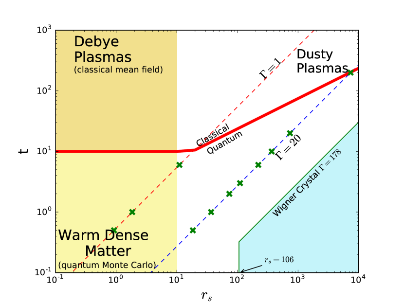
Figure 1: Values of $r_{s}$ and $t$ of interest. Note that the values correspond to a range of experimental conditions from electrons to dusty plasmas. A definition of the crossover to quantum effects from classical behavior is shown. Crosses indicate the conditions studied in sections III and IV.

The next section defines the effective classical description for the density profile in terms of the modified pair potential and confining potential - all quantum effects occur through modifications of the underlying Coulomb and harmonic forms, respectively. The approximate form for the pair potential is described in Appendix A. As noted above it has been shown to give good predictions for the pair correlation function of the uniform electron gas, in comparison to quantum Monte Carlo simulation DD13 . The choice for the modified confining potential is described in B, where the potential is represented in terms of a ”trial” quantum density imposing a known limit. Density profiles calculated on the basis of chosen quantum input are given in Sections III and IV for values of $t$ and $r_{s}$ corresponding to the line $\Gamma=20$ in Figure 1. The purely classical profile would be the same in all of these cases since it depends only on $\Gamma$. Hence the observed differences are purely quantum effects. Two choices for determination of the effect trap are explored here. The first is that whose trial density is the limit of non-interacting Fermions in a harmonic trap. At the highest values of $t$ and $r_{s}$ the classical limit is valid and at $\Gamma=20$ Coulomb correlations are strong enough for shell structure, well-known for dusty plasmas. At the smallest values of $t$ and $r_{s}$ a different shell structure emerges from extreme distortion of the non-interacting trial density due to exchange effects. The analysis for a second choice of the effective trap is repeated in Section IV with an improved trial density to include the effects of Coulomb interactions. With this quantum input, the new shell structure at small $t$ and $r_{s}$ no longer dominates and the quantum differences from the classical form are quantitative rather than qualitative. This sensitivity of the classical theory to the modifications of the confining potential, the need for guidance from simulation, and the outlook for future applications in materials sciences are discussed in the last section.

II Density Profile - Classical Map of the Quantum System

The Hamiltonian for $N$ particles with charge $q$ in a harmonic trap is

$$H-\mu N=\sum_{i=1}^{N}\frac{p_{i}^{2}}{2m}+\frac{1}{2}\sum_{i\neq j}^{N}\frac{q^{2}}{\left|\mathbf{r}_{i}-\mathbf{r}_{j}\right|}-\int d\mathbf{r}\mu(\mathbf{r})\widehat{n}(\mathbf{r}),$$ (1)

with the local chemical potential given explicitly as

$$\mu(\mathbf{r})=\mu-\frac{1}{2}m\omega^{2}r^{2},$$ (2)

and the operator $\widehat{n}(\mathbf{r})$ representing the microscopic density is

$$\widehat{n}(\mathbf{r})=\sum_{i=1}^{N}\delta\left(\mathbf{r}-\mathbf{q}_{i}\right).$$ (3)

The constant $\mu$ determines the average number of charges $\overline{N}$ at equilibrium in the grand canonical ensemble. As a consequence of the harmonic potential the equilibrium average density profile for the charges is non-uniform

$$n(\mathbf{r},\beta\mid\mu)=\Omega^{-1}\sum_{N=1}^{\infty}N\int d\mathbf{r}_{2}..d\mathbf{r}_{N}\left\langle\mathbf{r}..\mathbf{r}_{N}\right|e^{-\beta\left(H-\mu N\right)}\left|\mathbf{r}..\mathbf{r}_{N}\right\rangle,$$ (4)

where $\left\langle\mathbf{r}_{1}..\mathbf{r}_{N}\right|X\left|\mathbf{r}_{1}..\mathbf{r}_{N}\right\rangle$ is the $N$ particle diagonal, properly symmetrized (Fermions or Bosons) matrix element in coordinate representation, and $\Omega$ is the grand potential

$$\Omega(\beta\mid\mu)=\sum_{N=1}^{\infty}\int d\mathbf{r}_{1}..d\mathbf{r}_{N}\left\langle\mathbf{r}_{1}..\mathbf{r}_{N}\right|e^{-\beta\left(H-\mu N\right)}\left|\mathbf{r}_{1}..\mathbf{r}_{N}\right\rangle,$$ (5)

The notation $f(a,b\mid c)$ indicates a function of the parameters $a,b$ and a functional of $c\left(\mathbf{r}\right)$. The density profile in the classical limit has been studied in detail, via simulation and theory Wrighton . In that case the dimensionless form depends only on $\overline{N}$ and the Coulomb coupling constant $\Gamma=\beta q^{2}/r_{0}$. For sufficiently large Coulomb coupling, $\Gamma,$ the formation of shell structure is observed in $n(\mathbf{r})$. The objective here is to exploit this classical description to explore the effects of quantum diffraction and exchange via a proposed equivalent classical system DuftyDutta ; DuttaDufty . The equivalent classical system has an effective local chemical potential, $\mu_{c}(\mathbf{r})$, an effective pair potential, $\phi_{c}(\left|\mathbf{r}_{i}\mathbf{-r}_{j}\right|)$, and an effective inverse temperature, $\beta_{c}$. These must be given as functions of $\mu(\mathbf{r})$, $\phi(\left|\mathbf{r}_{i}\mathbf{-r}_{j}\right|)$, and $\beta$ for the quantum system

The basis for the classical study used here is the hypernetted chain (HNC) description for an inhomogeneous equilibrium system Attard89 , or Eq. (37) of reference DD13

$$\ln\left(n\left(\mathbf{r},\beta_{c}\mid\mu_{c}\right)\lambda_{c}^{3}\right)=\beta_{c}\mu_{c}(\mathbf{r})+\int d\mathbf{r}^{\prime}c^{(2)}(\mathbf{r,r}^{\prime},\beta_{c}\mid\mu_{c})n\left(\mathbf{r}^{\prime}\right),$$ (6)

where $\lambda_{c}=\left(2\pi\beta_{c}\hbar^{2}/m\right)^{1/2}$ is the thermal de Broglie wavelength expressed in terms of the effective classical temperature, and $c^{(2)}(\mathbf{r,r}^{\prime},\beta_{c}\mid\mu_{c})$ is the direct correlation function defined by the Ornstein-Zernicke equation in terms of the pair correlation function for the inhomogeneous system Attard89 . Further details of the origins for this equation in classical density functional theory are given in reference Wrighton . The classical studies made a further approximation to this expression, replacing the direct correlation function for the inhomogeneous system by that for a corresponding uniform one component plasma (OCP or jellium), $c^{(2)}(\mathbf{r,r}^{\prime},\beta_{c}\mid\mu_{c})\rightarrow c(\left|\mathbf{r-r}^{\prime}\right|,\beta_{c},\mu_{c})$. The results based on this approximation are found to be quite accurate except at very strong coupling. A partial theoretical basis for this approximation has been given Wrighton12 and it will be made here as well.

An equivalent Boltzmann form for the density is defined in terms of a dimensionless potential $U(\mathbf{r})$ defined by

$$n\left(\mathbf{r},\mu_{c},\beta_{c}\right)=\overline{N}\frac{e^{-U(\mathbf{r},\mu_{c},\beta_{c})}}{\int d\mathbf{r}^{\prime}e^{-U(\mathbf{r}^{\prime},\mu_{c},\beta_{c})}},$$ (7)

where (6) gives

$$U(\mathbf{r,}\mu_{c},\beta_{c})=-\nu_{c}(\mathbf{r})-\frac{\overline{N}}{\int d\mathbf{r}^{\prime}e^{-U(\mathbf{r}^{\prime},\mu_{c},\beta_{c})}}\int d\mathbf{r}^{\prime}e^{-U(\mathbf{r}^{\prime},\mu_{c},\beta_{c})}c(\left|\mathbf{r-r}^{\prime}\right|,\mu_{c},\beta_{c}).$$ (8)

The dimensionless activity, $\nu_{c}(\mathbf{r,}\mu_{c},\beta_{c})=\beta_{c}\mu_{c}(\mathbf{r})$, has been introduced in (8) and $c(r,\mu_{c},\beta_{c})$ is now the direct correlation function for the uniform OCP. For future reference, note that at fixed $\overline{N}$ the representation for $n\left(\mathbf{r}\right)$ is invariant to a shift of $\nu_{c}(\mathbf{r})$ by a constant. In the following applications this flexibility will be used to choose $U(\mathbf{0,}\mu_{c},\beta_{c})=0.$

Equations (7) and (8) are a classical representation for the density profile (4) for the underlying quantum system. The latter is parameterized by the total average number of particles $\overline{N}$, the inverse temperature $\beta$, and the chemical potential of the uniform system $\mu$. In the following, a change of variables from $\beta,\mu$ to $\beta,\overline{n}$ is considered, where $\overline{n}$ is the average density of the representative uniform system. To introduce the density, it is necessary to assign a volume for the system. This can be taken as the volume of a sphere with radius $R_{0}$ corresponding to a particle at the greatest distance from the center. At equilibrium the average fluid phase density is spherically symmetric so that the total average force on that particle is

$$\frac{\left(\overline{N}-1\right)q^{2}}{R_{0}^{2}}-m\omega^{2}R_{0}=0,\hskip 18.06749pt\Rightarrow R_{0}^{3}=\left(\overline{N}-1\right)\frac{q^{2}}{m\omega^{2}}.$$ (9)

This gives the average density to be

$$\overline{n}\equiv\frac{3\overline{N}}{4\pi R_{0}^{3}}=\frac{3m\omega^{2}}{4\pi q^{2}}\frac{\overline{N}}{\overline{N}-1}.$$ (10)

As expected the density is determined by the trap parameter $m\omega^{2}/q^{2}$. A corresponding length scale $r_{0}$ is the average distance between particles given by $4\pi r_{0}^{3}/3=1/\overline{n}$. The following dimensionless measures of distance, temperature, and density will be used

$$\mathbf{r}^{\ast}=\frac{r}{r_{0}},\hskip 14.45377ptt=\frac{1}{\beta\epsilon_{F}},\hskip 14.45377ptr_{s}=\frac{r_{0}}{a_{b}}.$$ (11)

Here $\epsilon_{F}$ is the Fermi energy and $a_{b}$ is the Bohr radius, both defined in terms of the mass and charge of the particles in the trap

$$\epsilon_{F}=\frac{1}{2m}\hbar^{2}\left(3\pi^{2}\overline{n}\right)^{2/3}=\left(\frac{m_{e}}{m}\right)\epsilon_{eF},\hskip 14.45377pta_{b}=\frac{\hbar^{2}}{mq^{2}}=\left(\frac{m_{e}e^{2}}{mq^{2}}\right)a_{B},$$ (12)

$$\nu(\mathbf{r,}\mu_{e},\beta)=\beta\mu_{e}-\frac{1}{2}\Gamma(t,r_{s})r^{\ast 2}$$ (13)

In the last equalities of (12) $\epsilon_{eF}$ and $a_{B}$ are the electron Fermi energy and the usual Bohr radius, respectively. The prefactor $m_{e}e^{2}/mq^{2}$ shows how the very large values of $r_{s}$ in Figure 1 can be obtained for particles of large mass and large charge.

Finally, define the reduced potential $u(\mathbf{r}^{\ast},t,r_{s})$, direct correlation function $\overline{c}(r^{\ast},t,r_{s})$, and local activity $\overline{\nu}_{c}(\mathbf{r}^{\ast},t,r_{s})$ by

$$U(\mathbf{r})=\Gamma_{e}(t,r_{s})u(\mathbf{r}^{\ast},t,r_{s}),\hskip 14.45377ptc(r,\mu_{c},\beta_{c})=\Gamma_{e}(t,r_{s})\overline{c}(r^{\ast},t,r_{s}),\hskip 14.45377pt\nu_{c}(\mathbf{r},\mu_{c},\beta_{c})=\Gamma_{e}(t,r_{s})\overline{\nu}_{c}(\mathbf{r}^{\ast},t,r_{s}).$$ (14)

An effective coupling constant $\Gamma_{e}(t,r_{s})$ has been extracted in each case

$$\Gamma_{e}\left(t,r_{s}\right)=\frac{2}{\beta\hbar\omega_{p}\coth\left(\beta\hbar\omega_{p}/2\right)}\Gamma,\hskip 14.45377pt\Gamma\equiv\frac{\beta q^{2}}{r_{0}}.$$ (15)

Here $\omega_{p}=\sqrt{4\pi\overline{n}q^{2}/m}$ is the plasma frequency. The dimensionless parameter is $\beta\hbar\omega_{p}=\left(4/3\right)\left(2\sqrt{3}/\pi^{2}\right)^{1/3}\sqrt{r_{s}}/t$ $\simeq 0.940\,52\sqrt{r_{s}}/t$ . At fixed $r_{s}$ and large $t$, $\Gamma_{e}\left(t,r_{s}\right)\rightarrow\Gamma\simeq 0.543r_{s}/t$ which is the classical Coulomb coupling constant. The motivation for introducing $\Gamma_{e}\left(t,r_{s}\right)$ is the fact that it represents the strength of the Coulomb tail for the effective classical pair potential DuttaDufty , as shown in Appendix A eq. (37). This means that the strength of the effective classical repulsion of particles in the trap is $\Gamma_{e}\left(t,r_{s}\right)$ while the strength of the harmonic containment is $\Gamma(t,r_{s})$ (see (13)). Since $\Gamma_{e}\left(t,r_{s}\right)$ decreases with increasing quantum effects, stronger confinement relative to the purely classical result is expected.

The dimensionless form for the density profile, from (7) and (8) is now

$$n^{\ast}\left(\mathbf{r}^{\ast},t,r_{s}\right)=n\left(\mathbf{r},\mu_{c},\beta_{c}\right)r_{0}^{3}=\overline{N}\frac{e^{-\Gamma_{e}(t,r_{s})u(\mathbf{r}^{\ast},t,r_{s})}}{\int d\mathbf{r}^{\ast\prime}e^{-\Gamma_{e}(t,r_{s})u(\mathbf{r}^{\ast\prime},t,r_{s})}},$$ (16)

$$u(\mathbf{r}^{\ast},t,r_{s})=-\overline{\nu}_{c}(\mathbf{r}^{\ast},t,r_{s})-\frac{\overline{N}}{\int d\mathbf{r}^{\ast\prime\prime}e^{-\Gamma_{e}(t,r_{s})u(\mathbf{r}^{\ast\prime\prime},t,r_{s})}}\int d\mathbf{r}^{\ast\prime}e^{-\Gamma_{e}(t,r_{s})u(\mathbf{r}^{\ast\prime},t,r_{s})}\overline{c}(\left|\mathbf{r}^{\ast}\mathbf{-r}^{\ast\prime}\right|,t,r_{s}).$$ (17)

Practical application requires specification of the direct correlation function $\overline{c}(r^{\ast},t,r_{s})$ for jellium and the classical activity $\overline{\nu}_{c}(r^{\ast},t,r_{s})$. The method for determining these is such that they are explicit functions of the dimensionless variables $t,r_{s}$ for the given quantum system, rather than of the associated classical parameters $\mu_{c},\beta_{c}$. Hence, the potentially confusing notation in (14). The former is determined from an accurate equivalent classical calculation described elsewhere DD13 and summarized in Appendix A. The direct correlation function is a classical concept whose quantum modifications here appear only through the effective pair potential. That potential is obtained in Appendix A and has two main changes from the underlying Coulomb potential due to quantum effects in the classical representation. The first is a regularization of the Coulomb singularity at the origin due to diffraction effects - the pair potential remains finite at zero separation. The second main change is the strength of the $1/r$ behavior at large distances, with the coupling constant $\Gamma$ being replaced by $\Gamma_{e}$ of (15).

The activity $\overline{\nu}_{c}(\mathbf{r}^{\ast},t,r_{s})$ describes the effective classical trap potential corresponding to the actual quantum harmonic trap, and its approximate determination is described in Appendix B. It is defined such that the density profile for a chosen quantum system is recovered in an appropriate limit. In this way the exact quantum effects of that limit are incorporated in the classical system and exploited approximately away from that limit as well. The resulting form for (16) and (17) obtained in Appendix B is

$$n^{\ast}\left(\mathbf{r}^{\ast},t,r_{s}\right)=N\frac{n_{T}^{\ast}\left(\mathbf{r}^{\ast},t,r_{s}\right)e^{\Gamma_{e}(t,r_{s})\Delta u(\mathbf{r}^{\ast}\mathbf{,}t,r_{s}\mid n)}}{\int d\mathbf{r}^{\prime}n_{T}^{\ast}\left(\mathbf{r}^{\ast\prime}\right)e^{\Gamma_{e}(t,r_{s})\Delta u(\mathbf{r}^{\ast\prime},,t,r_{s}\mid n)}}.$$ (18)

$$\Delta u(\mathbf{r}^{\ast}\mathbf{,}t,r_{s}\mid n)=\int d\mathbf{r}^{\prime}\left(\overline{c}(\left|\mathbf{r}^{\ast}\mathbf{-r}^{\ast\prime}\right|,t,r_{s})n^{\ast}\left(\mathbf{r}^{\ast\prime},t,r_{s}\right)-\overline{c}_{T}(\left|\mathbf{r}^{\ast}\mathbf{-r}^{\ast\prime}\right|,t,r_{s})n_{T}^{\ast}\left(\mathbf{r}^{\prime},t,r_{s}\right)\right).$$ (19)

Here $n_{T}^{\ast}\left(\mathbf{r}^{\ast},t,r_{s}\right)$ is the ”trial” quantum density profile enforcing the associated quantum limit for $n^{\ast}\left(\mathbf{r}^{\ast},t,r_{s}\right)$, and $\overline{c}_{T}(r^{\ast},t,r_{s})$ is the associated direct correlation function for that limit. See Appendix B for further details. Equations (18) and (19) are the basis for all the results reported here. Two cases are considered here, the limit of non-interacting Fermions in a harmonic trap, and the corresponding system with weak Coulomb interactions.

III Classical trap for non-interacting Fermions

For a first study of the quantum effects consider an effective trap whose classical density is the same as the quantum density of non-interacting Fermions in a harmonic trap. The corresponding trap density in (18) and (19) is denoted by $n_{T}^{\ast}(r^{\ast},t,r_{s})\rightarrow n^{\ast(0)}(r^{\ast},t,r_{s})$ and the direct correlation function for this case is denoted by $c_{T}(r^{\ast},t,r_{s})\rightarrow c^{(0)}(r^{\ast},t,r_{s})$. The former is calculated directly from

$$n^{\ast(0)}\left(\mathbf{r}^{\ast},t,r_{s}\right)=2r_{0}^{3}\left\langle\mathbf{r}\right|\left(e^{\left(\beta\frac{\widehat{p}^{2}}{2m}-\left(\nu_{0}-\frac{1}{2}m\omega^{2}\widehat{r}^{2}\right)\right)}+1\right)^{-1}\left|\mathbf{r}\right\rangle.$$ (20)

$\left\langle\mathbf{r}\right|X\left|\mathbf{r}\right\rangle$ denotes a diagonal matrix element in coordinate representation. It has been assumed that the system is comprised of unpolarized spin $1/2$ particles. A caret on a variable indicates it is the operator corresponding to that variable. The parameter $\nu_{0}$ is determined by the condition that the total average number of particles is the same as the interacting system

$$\overline{N}(t,r_{s})=2r_{0}^{-3}\int d\mathbf{r}\left\langle\mathbf{r}\right|\left(e^{\left(\beta\frac{\widehat{p}^{2}}{2m}-\left(\nu_{0}-\frac{1}{2}m\omega^{2}\widehat{r}^{2}\right)\right)}+1\right)^{-1}\left|\mathbf{r}\right\rangle.$$ (21)

Equations (20) and (21) can be evaluated in terms of the harmonic oscillator eigenfunctions and eigenvalues. Instead, here a local density (Thomas-Fermi) approximation is used. This follows from the replacement of the operator $\widehat{r}^{2}$ by the corresponding c-number $r^{2}$. Then the matrix element can be evaluated to give

$$n^{\ast(0)}\left(\mathbf{r}^{\ast}\right) \rightarrow\left(\frac{r_{0}}{\lambda}\right)^{3}\frac{4}{\sqrt{\pi}}I_{\frac{1}{2}}\left(\nu_{0}-\frac{1}{2}\Gamma(t,r_{s})r^{\ast 2}\right)\hskip 14.45377pt$$ (22)

$$\overline{N} =\left(\frac{r_{0}}{\lambda}\right)^{3}4\pi\int_{0}^{\infty}dr^{\ast}r^{\ast 2}\frac{4}{\sqrt{\pi}}I_{\frac{1}{2}}\left(\left(\nu_{0}-\frac{1}{2}\Gamma(t,r_{s})r^{\ast 2}\right)\right).$$ (23)

The Fermi function $I_{\alpha}\left(\beta\mu\right)$ and thermal de Broglie wavelength $\lambda$ are given by

$$I_{\alpha}\left(\beta\mu\right)=\int_{0}^{\infty}dx\frac{x^{\alpha}}{e^{x-\beta\mu}+1},\hskip 14.45377pt\lambda=\left(\frac{2\pi\hbar^{2}\beta}{m}\right)^{1/2}.$$ (24)

The validity of this Thomas-Fermi approximation for the conditions considered here ($\overline{N}=100$) is demonstrated in Appendix C.

The direct correlation function $c^{(0)}(r^{\ast},t,r_{s})$ is non-trivial because the classical system corresponding to a non-interacting quantum gas has pairwise interactions needed to reproduce the symmetrization effects. Hence calculation of properties for this effective classical system is a true many-body problem. The Ornstein-Zernicke equation is used, with the known exact quantum non-interacting pair correlation function $g^{(0)}(r)$ as input DuttaDufty

$$c^{(0)}\left(r^{\ast},t,r_{s}\right)=\left(g^{(0)}(r^{\ast},t,r_{s})-1\right)-\overline{n}\int d\mathbf{r}^{\ast\prime}c^{(0)}(\left|\mathbf{r}^{\ast}\mathbf{-r}^{\ast\prime}\right|,t,r_{s})\left(g^{(0)}(r^{\ast\prime},t,r_{s})-1\right).$$ (25)

Finally, the direct correlation function for the interacting system is calculated from the coupled HNC and Ornstein-Zernicke equations

$$\ln\left(g(r^{\ast},t,r_{s})\right)=-\phi_{c}^{\ast}(r^{\ast},t,r_{s})+\left(g(r^{\ast},t,r_{s})-1\right)-c\left(r^{\ast},t,r_{s}\right),$$ (26)

$$c\left(r^{\ast},t,r_{s}\right)=\left(g(r^{\ast},t,r_{s})-1\right)-\overline{n}\int d\mathbf{r}^{\prime}c(\left|\mathbf{r}^{\ast}\mathbf{-r}^{{}^{\ast}\prime}\right|,t,r_{s})\left(g(r^{\ast\prime},t,r_{s})-1\right).$$ (27)

Here $\phi_{c}^{\ast}(r^{\ast},t,r_{s})$ is the effective classical pair interaction representing the uniform electron gas, described in Appendix A.

Equations (18) and (19) for this case are now

$$n^{\ast}\left(r^{\ast},t,r_{s}\right)=N\frac{n^{\ast(0)}\left(r^{\ast},t,r_{s}\right)e^{\Gamma_{e}(t,r_{s})\Delta u(r^{\ast}\mathbf{,}t,r_{s}\mid n)}}{\int d\mathbf{r}^{\prime}n^{\ast(0)}\left(r^{\ast\prime}\right)e^{\Gamma_{e}(t,r_{s})\Delta u(\mathbf{r}^{\ast\prime},,t,r_{s}\mid n)}},$$ (28)

$$\Delta u(\mathbf{r}^{\ast}\mathbf{,}t,r_{s}\mid n)=\int d\mathbf{r}^{\prime}\left(\overline{c}(\left|\mathbf{r}^{\ast}\mathbf{-r}^{\ast\prime}\right|,t,r_{s})n^{\ast}\left(r^{\ast\prime},t,r_{s}\right)-\overline{c}^{(0)}(\left|\mathbf{r}^{\ast}\mathbf{-r}^{\ast\prime}\right|,t,r_{s})n^{\ast(0)}\left(r^{\ast\prime},t,r_{s}\right)\right).$$ (29)

The quantum input for this classical description is two-fold. The first is a modification of the Coulomb interactions among charges via $\phi_{c}^{\ast}(r^{\ast},t,r_{s})$, due to both diffraction and exchange effects. These occur through the direct correlations $\overline{c}(r^{\ast},t,r_{s})$. Additional quantum effects occur due to the modification of the shape and intensity of the harmonic trap. These occur through $n^{\ast(0)}\left(r^{\ast},t,r_{s}\right)$. To explore these a series of density profiles  is shown in Figure 2 for values of $t,r_{s\text{ }}$corresponding to the line $\Gamma=20$ in Figure 1. Without quantum effects all profiles would be the same as the classical limit shown. The observed classical shell structure in that case is due entirely to strong Coulomb coupling with no quantum effects. As the values of $t,r_{s\text{ }}$ are decreased this Coulomb shell is distorted and shifted inward, corresponding to a weakening of the Coulomb repulsion through a decreasing effective coupling $\Gamma_{e}(t,r_{s})$. This weakening of Coulomb correlations in $c(r^{\ast},t,r_{s})$ is displayed in Figure 3a. The direct correlation function has quantum effects that enter the HNC theory only through the effective pair potential (Appendix A). The latter has a Coulomb tail whose amplitude is decreased by $\Gamma_{e}/\Gamma$ so that long range correlations are weakened. At shorter distances the Coulomb singularity is removed in the effective pair potential due to diffraction effects. The classical direct correlation function is finite at $\mathbf{r}^{\ast}=0$ for sufficiently strong coupling due to Coulomb correlations in spite of the singular Coulomb potential. However, with quantum diffraction effects the effective pair potential is non-singular and the direct correlation function remains finite $\mathbf{r}^{\ast}=0$ even at weak coupling. These qualitative changes are illustrated for three cases in Figure 3a corresponding to $t=200,20,$ and $2$ in Figure 2. The smaller values at $\mathbf{r}^{\ast}=0$ tend to enhance shell formation while the weaker coupling of $\Gamma_{e}/\Gamma$ tends to decrease it.

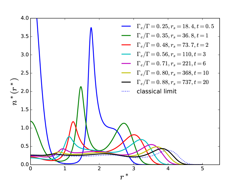
Figure 2: Onset of quantum effects for a system of 100 particles. Here $\Gamma=20$ as temperature decreases from $t=20$ to $t=0.5$.

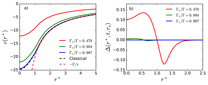
Figure 3: Two quantum effects for $\Gamma=20$. a) Quantum effect on the direct correlation function. The negative of the Coulomb potential is also shown for reference. b) Quantum effect on the shape of the trapping potential near the origin.

A qualitatively new consequence of quantum effects occurs at the lowest value of $t=0.5$ and $r_{s}=18.4$. A strong single shell occurs that is unrelated to the classical Coulomb shell structure and is due entirely to a change in shape of the confining potential. To be more explicit, write the confining potential, or equivalently $\overline{\nu}_{c}(\mathbf{r}^{\ast},t,r_{s})$, as

$$\overline{\nu}_{c}^{(0)}(\mathbf{r}^{\ast},t,r_{s})-\overline{\nu}_{c}^{(0)}(\mathbf{0},t,r_{s})=\frac{\Gamma}{\Gamma_{e}}\frac{1}{2}\mathbf{r}^{\ast 2}+\Delta\left(\mathbf{r}^{\ast},t,r_{s}\right).$$ (30)

There are two quantum effects evident in this form, an increase in amplitude of the harmonic potential by $\Gamma/\Gamma_{e}$, and a change in shape represented by $\Delta\left(\mathbf{r}^{\ast},t,r_{s}\right)$. The change in amplitude of the harmonic potential is a reflection of its enhancement relative to $\overline{c}(r^{\ast},t,r_{s})$ and is largely responsible for the increased confinement observed in all density profiles of Figure 2. As the shells are pulled inwards, this also tends to cause a population transfer to the outer shell. However, at the lowest temperatures the change in shape from the harmonic form becomes large. It is this distortion that is responsible for the onset of the new shell structure seen in Figure 2. This is confirmed in Figure 4 which shows the superposition of the shell and the local distortion of the confining potential relative to its harmonic form. The origin of this distortion is the Fermi statistics of the non-interacting particles which force the trap density to go to zero at a finite radius as $t\rightarrow 0$ (Appendix B). This translates into a hard wall for the effective confining potential, and an associated shell structure (even in a classical fluid hard wall confinement leads to shell structure). The predicted location of the $t=0$ wall in Appendix B is $1.77$, very close to that observed in Figure 4 at $t=0.5$.

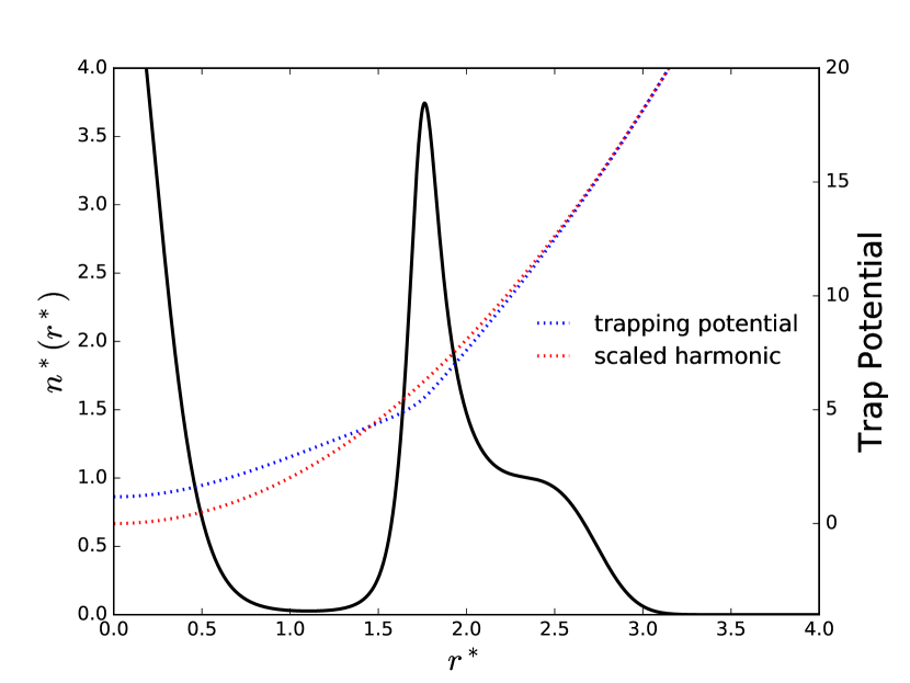
Figure 4: The low temperature quantum effect of the trapping potential on the density $n(r)$. The system is strongly coupled ($\Gamma=20$) with $r_{s}=18.4$ and $t=0.5$. The scaled harmonic function is shown, as well as the full trapping potential.

IV Classical trap with weak Coulomb interactions

Now consider the same analysis based on (18) and (19), but with a better choice for the effective confining potential to include some effects of the Coulomb interactions on the classical confining potential.  This change does not affect $\overline{c}(r^{\ast},t,r_{s})$, which is the same as in the previous section. The new choice is defined by imposing a weak coupling limit for which the corresponding trap density is obtained from a quantum density functional calculation including Hartree and exchange interactions in a local density approximation, $n_{T}^{\ast}\left(\mathbf{r}^{\ast},t,r_{s}\right)\rightarrow n^{\ast\left(w\right)}\left(\mathbf{r}^{\ast},t,r_{s}\right)$ given by (56). The details are discussed in Appendix B.2. Accordingly, the corresponding classical limit for the trial direct correlation function is its weak coupling expansion to first order in $\Gamma$, $\overline{c}_{T}(r^{\ast},t,r_{s})\rightarrow\overline{c}^{(0)}(r^{\ast},t,r_{s})+\Gamma\overline{c}^{(1)}(r^{\ast},t,r_{s})$, and (18) and (19) become

$$n^{\ast}\left(\mathbf{r}^{\ast},t,r_{s}\right)=\overline{N}\frac{n^{\ast\left(w\right)}\left(\mathbf{r}^{\ast},t,r_{s}\right)e^{\Gamma_{e}(t,r_{s})\Delta u(\mathbf{r}^{\ast}\mathbf{,}t,r_{s}\mid n)}}{\int d\mathbf{r}^{\prime}n^{\ast\left(w\right)}\left(\mathbf{r}^{\ast\prime}\right)e^{\Gamma_{e}(t,r_{s})\Delta u(\mathbf{r}^{\ast\prime},,t,r_{s}\mid n)}}.$$ (31)

$$\Delta u(\mathbf{r}^{\ast}\mathbf{,}t,r_{s} \mid n)=\int d\mathbf{r}^{\prime}\left(\overline{c}(\left|\mathbf{r}^{\ast}\mathbf{-r}^{\ast\prime}\right|,t,r_{s})n^{\ast}\left(\mathbf{r}^{\ast\prime},t,r_{s}\right)\right.$$

$$\left.-\left(\overline{c}^{(0)}(\left|\mathbf{r}^{\ast}\mathbf{-r}^{\ast\prime}\right|,t,r_{s})+\Gamma\overline{c}^{(1)}(\left|\mathbf{r}^{\ast}\mathbf{-r}^{\ast\prime}\right|,t,r_{s})\right)n^{\ast\left(w\right)}\left(\mathbf{r}^{\prime},t,r_{s}\right)\right)$$ (32)

The direct correlation functions $\overline{c}(r^{\ast},t,r_{s})$ and $\overline{c}^{(0)}(r^{\ast},t,r_{s})$ are again calculated in the HNC approximation using (25) - (27). Also, the weak coupling coefficient $\overline{c}^{(1)}(r^{\ast},t,r_{s})$ is obtained numerically from these equations for asymptotically small $\Gamma$.

Figure 5 shows the density profiles for the same temperatures as in Figure 2 along the line $\Gamma=20$ in Figure 1. The results are quite similar at the high temperatures, e.g. $t=20$, as the classical limit is approached. However, at all lower temperatures there is a qualitative difference between Figures 5 and 2. In the latter case the intermediate peak diminishes and the new shell at small $r^{\ast}$ grows as the temperature decreases until a single dominant peak is formed at the lowest temperature. In contrast, the outer and intermediate peaks of Figure 5 change in a unified fashion as the overall density profile contracts with decreasing temperature. The two peak structure is maintained with only quantitative changes occurring due to quantum effects - no new shell structure is seen as in Figure 2. As indicated in (30), the quantum effects on the confining potential are an enhancement of the harmonic form and a distortion of that form. The distortion $\Delta\left(\mathbf{r}^{\ast},t,r_{s}\right)$ is now very much decreased by the inclusion of weak Coulomb interactions in the determination of the classical confining potential, eliminating the new ”hard wall” shell structure of Figure 2. This is illustrated in Figure 6 for $t=0.5$.

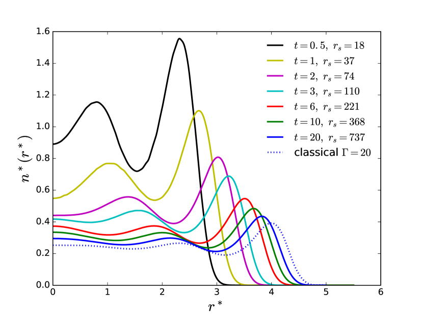
Figure 5: Onset of quantum effects for a system of 100 particles. Here $\Gamma=20$ as temperature decreases from $t=20$ to $t=0.5$.

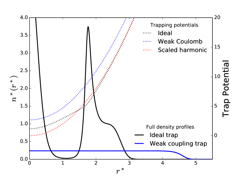
Figure 6: Effect of including weak Coulomb interactions on trapping potential distortion. Black dashed line is the distorted trapping potential for non-interacting particles. Blue dashed line is the distorted trapping potential when weak Coulomb interactions are included. For reference, the red dashed line shows the scaled harmonic potential $\frac{1}{2}\frac{\Gamma}{\Gamma_{e}}r^{*2}$ with no shape distortion. Here $t=0.5$ and $\Gamma=20$.

The quantum effects on the amplitude and location of the shells in Figure 5 are quite significant. For example, at $t=1$ the outer peak increases by a factor of 2.8 relative to the classical value. The contraction is largely due to the factor $\Gamma(t,r_{s})/\Gamma_{e}(t,r_{s})$ which changes from $1.13$ at $t=20$ to $2.86$ at $t=1$. The results discussed thus far are all for the strong coupling condition $\Gamma=20$. This was chosen because shell structure is present for these conditions even in the classical limit. It is instructive now to consider the case $\Gamma=1$ for which there is no classical shell structure. Figure 7 shows the results for $t=6,1,$ and $0.5$. In contrast to the strong coupling case, $t=6$ is very close to the classical limit. The contraction of the profile is the dominant quantum effect at lower temperatures, and there is no shell structure evident in any case.

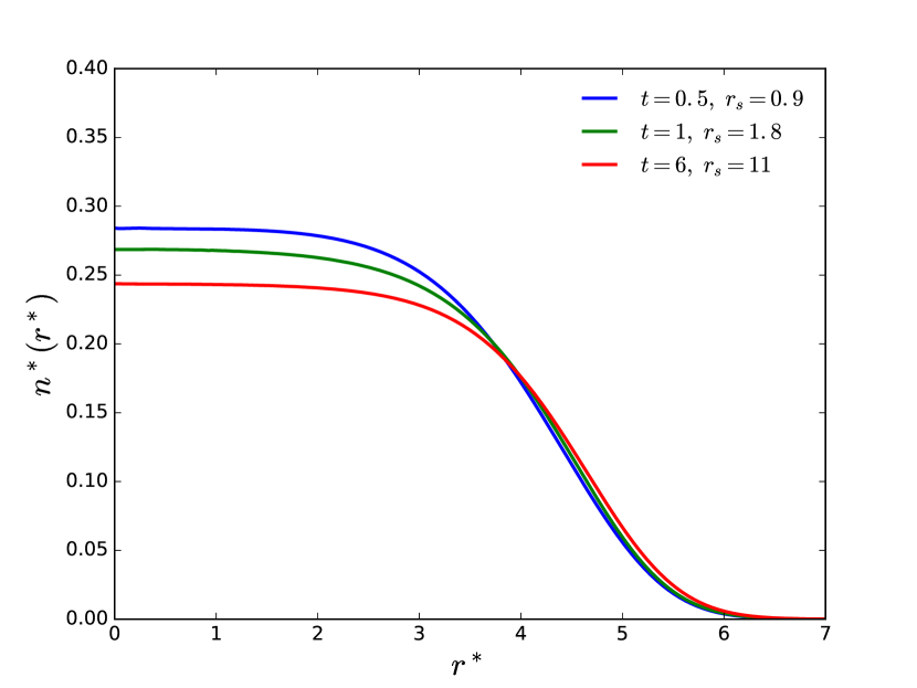
Figure 7: Density profiles for low temperatures ($t=0.5,1,6$) at $\Gamma=1$ for weak Coulomb interactions. No shell structure is formed at small temperatures for the weakly coupled case.

V Discussion

The classical shell structure for strong coupling conditions in the upper right corner of Figure 1 has provided a wealth of insight into formation of shell structure due to Coulomb correlations. Here these studies have been extended in the direction of additional quantum effects. The method chosen, an equivalent quantum system, allows inclusion of the diverse classical effects into an extension via effective pair potentials and effective confinement potentials. The quantum effects are included in the modification of these potentials from their classical Coulomb and harmonic forms in a controlled way defined by the formalism of references DuftyDutta ; DuttaDufty . Two approximate implementations of that formalism have been described. In both, the pair correlations among charges expressed by the direct correlation function $\overline{c}(r^{\ast},t,r_{s})$ are calculated from the classical HNC liquid state theory, known to be accurate for strong correlations, e.g. $\Gamma=20.$ The qualitative effects of quantum mechanics are illustrated in Figure 3a. The first approximation for the effective confining potential is that which gives the exact quantum density profile for non-interacting charges. The result is a scaling of the original harmonic trap by a factor $\Gamma(t,r_{s})/\Gamma_{e}(t,r_{s})$ which tends to increase the confinement relative to the Coulomb correlations. In addition there is a distortion of the harmonic form at low temperatures that produces a ”hard wall” associated with the vanishing of the non-interacting density at a finite value of $r^{\ast}$. This leads to a new shell structure not related to Coulomb correlations.

The second choice for the confining potential, described in Section IV, is that which gives the density profile for a weak coupling quantum density functional calculation. This potential includes the effects of Coulomb interactions. It has a similar scaling of the harmonic form, but no longer shows the strong distortion (compare Figures 3b and 6) and hence no new shell structure. In fact the profiles of Figure 5 at $\Gamma=20$ appear like a self-similar contraction constrained by the normalization to $\overline{N}=100$. The choice of parameters $\Gamma=20,\overline{N}=100$ was made to insure multiple shells in the reference classical limit. The brief consideration of $\Gamma=1,\overline{N}=100$ in Figure 7 confirms that there is no new shell structure induced solely by quantum effects.

Clearly there is more to be done with this classical description of a quantum system, such as $t<0.5$ and much smaller $\overline{N}$ to make direct connection with the literature on quantum dots. Presumably, for such conditions the local density approximation will need to be relaxed. A different direction for application is the replacement of the harmonic trap by a Coulomb potential to calculate the electron distribution about an ion. This is the first step in addressing the more practical case of determining the electronic configuration in a distribution of ionic sources. Such configurations are required to compute the forces in quantum molecular dynamics simulations for the ions in warm, dense matter at finite temperatures where traditional density functional methods fail WDM .

VI Acknowledgements

The authors are indebted to Michael Bonitz for his comments on an earlier draft. This research has been supported in part by NSF/DOE Partnership in Basic Plasma Science and Engineering award DE-FG02-07ER54946 and by US DOE Grant DE-SC0002139.

Appendix A Effective Classical Direct Correlation Function

The density profile for charges in a trap is governed by both the confining potential and the correlations among the particles in the trap. The latter appear in (19) via the direct correlation function $c(r,\mu_{c},\beta_{c})=\Gamma_{e}(t,r_{s})\overline{c}(r^{\ast},t,r_{s})$. In this appendix, the approximate evaluation of these correlations from the HNC integral equations of liquid state theory Hansen using an effective pair potential is summarized.

As noted in Section II, the correlations for the non-uniform charges in the trap are approximated by those for a uniform electron gas. The calculation of these correlations from an effective classical system has been described in some detail elsewhere DuftyDutta , so only the relevant equations are reproduced here for completeness. The approximate effective pair potential used there is

$$\phi_{c}^{\ast}(r^{\ast},t,r_{s})=\beta_{c}\phi_{c}(r)=\phi_{c}^{\ast(0)}(r^{\ast},t,r_{s})+\frac{1}{n}\int\frac{d\mathbf{k}}{\left(2\pi\right)^{3}}e^{-i\mathbf{k\cdot r}}\left(\frac{1}{S^{RPA}(k)}-\frac{1}{S^{(0)}(k)}\right).$$ (33)

Here $S^{RPA}(k)$ and $S^{(0)}(k)$ are the static structure factor for the random phase approximation and ideal gas, respectively. The first term $\left(\beta_{c}\phi_{c}(r)\right)^{(0)}$ is the effective potential for the ideal quantum gas obtained by inverting the coupled ideal gas HNC equations Hansen , i.e. eqs. (26) and (27) specialized to the ideal gas

$$\ln\left(g^{(0)}(r^{\ast},t,r_{s})\right)=-\phi_{c}^{\ast(0)}(r^{\ast},t,r_{s})+\left(g^{(0)}(r^{\ast},t,r_{s})-1\right)-c^{(0)}\left(r^{\ast},t,r_{s}\right),$$ (34)

$$c^{(0)}\left(r^{\ast},t,r_{s}\right)=\left(g^{(0)}(r^{\ast},t,r_{s})-1\right)-\overline{n}\int d\mathbf{r}^{\prime}c^{(0)}(\left|\mathbf{r}^{\ast}\mathbf{-r}^{{}^{\ast}\prime}\right|,t,r_{s})\left(g^{(0)}(r^{\ast\prime},t,r_{s})-1\right),$$ (35)

using the known exact ideal gas pair correlation function for $g^{(0)}(r,t,r_{s})$. Finally, with $\phi_{c}^{\ast}(r^{\ast},t,r_{s})$ determined in this way the direct correlation function for the interacting system is calculated from the full coupled HNC equations (26) and (27).

As a practical matter, a simplified representation of (33) has been proposed DD13 . The ideal gas contribution $\phi_{c}^{\ast\left(0\right)}(r^{\ast},t,r_{s})$ is the same, but the contribution from the Coulomb interactions is modeled by the exact low density, weak coupling functional form first derived by Kelbg Kelbg . Here that form is parameterized to include the exact low density value for the pair correlation function at $r=0$ Filinov04 , and the large $r$ behavior of the more complete form (33)

$$\phi_{c}^{\ast}(r^{\ast},t,r_{s})\simeq\phi_{c}^{\ast(0)}(r^{\ast},t,r_{s})+\Delta_{K}^{\ast}\left(r^{\ast},\Gamma_{e},r_{s}\right),$$ (36)

with

$$\Delta_{K}^{\ast}\left(r^{\ast},\Gamma_{e},r_{s}\right)\equiv\frac{\Gamma_{e}}{r^{\ast}}\left(1-\exp(-\left(ar^{\ast}\right)^{2})+\sqrt{\pi}\frac{ar^{\ast}}{\gamma}\operatorname{erfc}(\gamma ar^{\ast})\right).$$ (37)

Here

$$a=\left(r_{s}/\Gamma_{e}\right)^{1/2},\hskip 14.45377pt\gamma\left(\Gamma_{e}r_{s}\right)=-\frac{\left(\pi\Gamma_{e}r_{s}\right)^{1/2}}{\mathrm{\ln}s(\Gamma_{e}r_{s})},$$ (38)

and $s(\Gamma_{e}r_{s})$ is the two electron relative coordinate Slater sum at $r^{\ast}=0$

$$s(\Gamma_{e}r_{s})=-4\left(\pi\Gamma_{e}r_{s}\right)^{1/2}\int_{0}^{\infty}dye^{-y^{2}}\frac{y}{1-e^{\pi\left(\Gamma_{e}r_{s}\right)^{1/2}/y}}.$$ (39)

Also $\Gamma_{e}$ is the effective coupling constant of (15). Clearly, (36) has the computational advantage that $\Delta_{K}^{\ast}\left(r^{\ast},\Gamma_{e},r_{s}\right)$ is an explicit, analytic function of the input parameters $t,r_{s}$. The results obtained for correlations using (36) are quite similar to those obtained using (33).

Appendix B Effective Classical Trap Potential

The effective classical description of the local density for charges confined in a harmonic trap is given by DuftyDutta ; DuttaDufty

$$\ln\left(n\left(\mathbf{r}\right)\lambda_{c}^{3}\right)=\left(\beta_{c}\mu_{ec}-\beta_{c}v_{c}(\mathbf{r})\right)+\int d\mathbf{r}^{\prime}c(\left|\mathbf{r-r}^{\prime}\right|,\mu_{c},\beta_{c})n\left(\mathbf{r}^{\prime}\right).$$ (40)

where $n\left(\mathbf{r}\right)$ is the desired charge density and $c(\left|\mathbf{r-r}^{\prime}\right|,\mu_{c},\beta_{c})$ is the direct correlation function for the homogeneous electron gas calculated as described in Appendix A. To complete the description it is necessary to choose the effective trap potential and chemical potential, i.e. $\left(\beta_{c}\mu_{ec}-\beta_{c}v_{c}(\mathbf{r})\right).$ This is done by requiring that the effective trap reproduce a chosen approximate quantum density valid in some limit. In this way, some limiting quantum information is provided via the effective trap.

It is useful to express (41) in the equivalent form (7) that includes the normalization explicitly

$$n\left(\mathbf{r},\mu_{c},\beta_{c}\right)=\overline{N}\frac{e^{-U(\mathbf{r},\mu_{c},\beta_{c})}}{\int d\mathbf{r}^{\prime}e^{-U(\mathbf{r}^{\prime},\mu_{c},\beta_{c})}},$$ (41)

$$U(\mathbf{r,}\mu_{c},\beta_{c})=-\nu_{c}(\mathbf{r,}\mu_{c},\beta_{c})-\frac{\overline{N}}{\int d\mathbf{r}^{\prime}e^{-U(\mathbf{r}^{\prime},\mu_{c},\beta_{c})}}\int d\mathbf{r}^{\prime}e^{-U(\mathbf{r}^{\prime},\mu_{c},\beta_{c})}c(\left|\mathbf{r-r}^{\prime}\right|,\mu_{c},\beta_{c}).$$ (42)

Recall the notation that $\nu_{c}(\mathbf{r,}\mu_{c},\beta_{c})=\beta_{c}\mu_{c}(\mathbf{r})=$ $\beta_{c}\mu_{ec}-\beta_{c}v_{c}(\mathbf{r})$.

Let $\left(\beta_{c}\mu_{ec}-\beta_{c}v_{c}(\mathbf{r})\right)_{T}$ denote the effective trap potential and chemical potential in some chosen limit. The density profile in that limit, $n_{T}\left(\mathbf{r},\mu_{c},\beta_{c}\right),$ is therefore

$$\ln\left(n_{T}\left(\mathbf{r},\mu_{c},\beta_{c}\right)\lambda_{c}^{3}\right)=\left(\beta_{c}\mu_{ec}-\beta_{c}v_{c}(\mathbf{r})\right)_{T}+\int d\mathbf{r}^{\prime}c_{T}(\left|\mathbf{r-r}^{\prime}\right|,\mu_{c},\beta_{c})n_{T}\left(\mathbf{r}^{\prime},\mu_{c},\beta_{c}\right).$$ (43)

Here $c_{T}(r,\mu_{c},\beta_{c})$ is the direct correlation function corresponding in the classical form to the quantum limit considered. The limit must be such that an independent quantum calculation of $n_{T}\left(\mathbf{r},\mu_{c},\beta_{c}\right)$ can be implemented practically, and the corresponding $c_{T}(r,\mu_{c},\beta_{c})$ can be identified. Then with $c_{T}(r,\mu_{c},\beta_{c})$ and $n_{T}\left(\mathbf{r},\mu_{c},\beta_{c}\right)$ known, equation (43) defines the effective classical trap that gives the exact quantum density in the limit considered. The choice for the approximate effective trap in (40) is now made as

$$\left(\beta_{c}\mu_{ec}-\beta_{c}v_{c}(\mathbf{r})\right)\rightarrow\left(\beta_{c}\mu_{ec}-\beta_{c}v_{c}(\mathbf{r})\right)_{T}.$$ (44)

This assures the exact behavior $n_{T}\left(\mathbf{r},\mu_{c},\beta_{c}\right)$ is recovered in the appropriate limit. With this choice (41) and (42) become

$$n\left(\mathbf{r},\mu_{c},\beta_{c}\right)=N\frac{n_{T}\left(\mathbf{r},\mu_{c},\beta_{c}\right)e^{\Delta U(\mathbf{r},\mu_{c},\beta_{c}\mid n)}}{\int d\mathbf{r}^{\prime}n_{T}\left(\mathbf{r}^{\prime}\right)e^{\Delta U(\mathbf{r}^{\prime},\mu_{c},\beta_{c}\mid n)}}.$$ (45)

$$\Delta U(\mathbf{r},\mu_{c},\beta_{c}\mid n)=\int d\mathbf{r}^{\prime}\left(c(\left|\mathbf{r-r}^{\prime}\right|,\mu_{c},\beta_{c})n\left(\mathbf{r}^{\prime},\mu_{c},\beta_{c}\right)-c_{T}(\left|\mathbf{r-r}^{\prime}\right|,\mu_{c},\beta_{c})n_{T}\left(\mathbf{r}^{\prime},\mu_{c},\beta_{c}\right)\right).$$ (46)

Here it has been required that $\int d\mathbf{r}n_{T}\left(\mathbf{r},\mu_{c},\beta_{c}\right)=\overline{N}$. Equations (18) and (19) are the dimensionless forms of (45) and (46) quoted in the text.

B.1 Non-interacting charges limit

The simplest choice for an imposed limit by the confining potential is that for non-interacting charges in a harmonic trap. This choice properly includes the non-classical effects of exchange symmetry. The density in this case $n_{T}^{\ast}(r^{\ast},t,r_{s})\rightarrow n^{\ast(0)}(r^{\ast},t,r_{s})$ is given by the matrix element in (20), which can be evaluated directly as a sum over eigenfunctions $\psi_{\alpha}\left(\mathbf{r}\right)$ and eigenvalues $\epsilon_{\alpha}$ of the harmonic oscillator Hamiltonian

$$n_{T}^{(0)}\left(\mathbf{r},\mu_{c},\beta_{c}\right)=\sum_{\alpha}\left|\psi_{\alpha}\left(\mathbf{r}\right)\right|^{2}\left(e^{\left(\beta\epsilon_{\alpha}-\nu_{0}\right)}+1\right)^{-1}.$$ (47)

The activity $\nu_{0}$ is determined by the condition that the density integrate to $\overline{N}$. A simpler practical approximation is given by the Thomas-Fermi or local density approximation

$$n^{(0)}(\mathbf{r},\mu_{c},\beta_{c}) \simeq\frac{2}{h^{3}}\int d\mathbf{p}\left(e^{-\nu_{0}}e^{\beta\left(\frac{p^{2}}{2m}+v(r)\right)}+1\right)^{-1}$$

$$=\lambda^{-3}\frac{4}{\sqrt{\pi}}I_{\frac{1}{2}}(\nu_{0}-\beta v(\mathbf{r}))$$ (48)

where $v(r)$ is the harmonic trap potential, and the Fermi function $I_{\alpha}\left(\nu_{0}\right)$ and thermal de Broglie wavelength $\lambda$ are defined by

$$I_{\alpha}\left(\nu_{0}\right)=\int_{0}^{\infty}dx\frac{x^{\alpha}}{e^{x-\nu_{0}}+1},\hskip 14.45377pt\lambda=\left(\frac{2\pi\hbar^{2}\beta}{m}\right)^{1/2}.$$ (49)

The validity of this Thomas-Fermi approximation for the conditions considered here is demonstrated in Appendix C.

With this choice for the reference density (45) and (46) becomes

$$n\left(\mathbf{r},\mu_{c},\beta_{c}\right)=N\frac{n^{(0)}\left(\mathbf{r}\right)e^{\Delta U(\mathbf{r},\mu_{c},\beta_{c}\mid n)}}{\int d\mathbf{r}^{\prime}n^{(0)}\left(\mathbf{r}^{\prime}\right)e^{\Delta U(\mathbf{r}^{\prime},\mu_{c},\beta_{c}\mid n)}},$$ (50)

$$\Delta U(\mathbf{r},\mu_{c},\beta_{c}\mid n)=\int d\mathbf{r}^{\prime}\left(c(\left|\mathbf{r-r}^{\prime}\right|,\mu_{c},\beta_{c})n\left(\mathbf{r}^{\prime},\mu_{c},\beta_{c}\right)-c^{(0)}(\left|\mathbf{r-r}^{\prime}\right|,\mu_{c},\beta_{c})n^{(0)}\left(\mathbf{r}^{\prime},\mu_{c},\beta_{c}\right)\right).$$ (51)

where $c_{T}(r,\mu_{c},\beta_{c})\rightarrow c^{(0)}(r,\mu_{c},\beta_{c})$ corresponding to the non-interacting limit. Clearly, $n\left(\mathbf{r},\mu_{c},\beta_{c}\right)\rightarrow n^{(0)}\left(\mathbf{r},\mu_{c},\beta_{c}\right)$ in the absence of Coulomb interactions. Although it is not needed for calculation of (50), the effective trap potential is determined from

$$\beta_{c}\left(\mu_{ec}-v_{c}(\mathbf{r})\right)^{(0)}=\ln\left(n^{(0)}\left(\mathbf{r}\right)\lambda_{c}^{3}\right)+\int d\mathbf{r}^{\prime}c^{(0)}(\left|\mathbf{r-r}^{\prime}\right|,\mu_{c},\beta_{c})n^{(0)}\left(\mathbf{r}^{\prime},\mu_{c},\beta_{c}\right).$$ (52)

This is used in the calculations for Figure 3b.

It is instructive to look at the limit of zero temperature. A Sommerfeld expansion of the local density (48) gives

$$n^{\ast(0)}\left(\mathbf{r}^{\ast},t=0,r_{s}\right)=\left\{\begin{array}[c]{c}0.034r_{s}^{3/2}\left(\frac{2\nu_{0}}{\Gamma}-r^{\ast 2}\right)^{3/2},\hskip 14.45377ptr^{\ast}<\sqrt{\frac{2\nu_{0}}{\Gamma}}\\ 0,\hskip 14.45377ptr^{\ast}\geq\sqrt{\frac{2\nu_{0}}{\Gamma}}\end{array}\right.,$$ (53)

where $t\nu_{0}$ is determined from normalization

$$\nu_{0}=0.783\overline{N}^{1/3}\frac{r_{s}^{1/2}}{t},\hskip 14.45377pt\frac{2\nu_{0}}{\Gamma}=2.88\frac{\overline{N}^{1/3}}{r_{s}^{1/2}}.$$ (54)

The density is  concave from the origin until $r^{\ast}=\sqrt{2.88\frac{\overline{N}^{1/3}}{r_{s}^{1/2}}}$, beyond which it vanishes. This vanishing of the density implies that the associated effective classical confining potential develops a hard wall. For the case of Figure 4, $\overline{N}=100,r_{s}=18.4$, this gives $r^{\ast}\simeq 1.77$. The shell structure of Figures 2 and 4 are finite temperature precursors of this limit.

With $n^{\ast(0)}\left(\mathbf{r}^{\ast},t=0,r_{s}\right)$ known, the effective confining potential can be determined from (51), where the exact Fourier transform of the ideal gas direct correlation function has the simple form Amovilli07

$$\widetilde{c}^{(0)}(k^{\ast},t=0,r_{s})=r_{0}^{3}\left(1-\frac{1}{\frac{3}{4k_{F}^{\ast}}k^{\ast}-\frac{1}{16k_{F}^{\ast}}k^{\ast 3}}\right).$$ (55)

Here $k_{F}^{\ast}=k_{F}r_{0}=(9\pi/4)^{1/3}$ and $k_{F}=(3\pi^{2}n)^{1/3}$ is the Fermi wavelength.

B.2 Weak Coulomb limit

The non-interacting limit of the previous subsection has only exchange correlations among the particles to provide quantum effects on the effective trap. A better limit, incorporating some mean field Coulomb interactions as well is given by the weak Coulomb coupling approximation in density functional theory (Hartree plus exchange). Within the same Thomas-Fermi approximation as (48) this is

$$n_{T}\left(\mathbf{r},\mu_{c},\beta_{c}\right) \rightarrow n^{\left(w\right)}(\mathbf{r},\mu_{c},\beta_{c})\equiv\frac{2}{h^{3}}\int d\mathbf{p}\left(e^{-\nu_{0}}e^{\left(\beta\left(\frac{p^{2}}{2m}+v(\mathbf{r})\right)+\beta v^{\left(w\right)}(\mathbf{r})\right)}+1\right)^{-1}$$

$$=\lambda^{-3}\frac{4}{\sqrt{\pi}}I_{\frac{1}{2}}\left(\left(\nu_{0}-\beta v(\mathbf{r})-\beta v^{\left(w\right)}(\mathbf{r})\right)\right).$$ (56)

The potential $v^{\left(w\right)}(\mathbf{r})$ representing the effects of Coulomb interactions among the particles is given by

$$v^{\left(w\right)}(\mathbf{r})=q^{2}\int d\mathbf{r}^{\prime}\frac{n^{\left(w\right)}\left(\mathbf{r}^{\prime}\right)}{\left|\mathbf{r}-\mathbf{r}^{\prime}\right|}+v_{x}(n^{\left(w\right)}\left(\mathbf{r}\right)).$$ (57)

The first term is the mean-field Coulomb contribution (Hartree), while the second term $v_{x}(n\left(\mathbf{r}\right))$ is the local density approximation for exchange (density derivative of the exchange free energy Perrot79 )

$$v_{x}(n\left(\mathbf{r}\right))=-\frac{e^{2}}{\sqrt{\pi}\lambda}I_{-\frac{1}{2}}\left(\nu_{0}\left(\mathbf{r}\right)\right).$$ (58)

The density dependence of $v_{x}\left(n\right)$ is determined by inverting the ideal gas relationship

$$n(\mathbf{r})=\lambda^{-3}\frac{4}{\sqrt{\pi}}I_{\frac{1}{2}}\left(\nu_{0}(\mathbf{r})\right).$$ (59)

It remains to determine the corresponding approximation to the classical direct correlation function, $c_{T}\rightarrow c^{\left(w\right)}$. Since (57) results from an expansion of the Kohn-Sham potential to leading order in the Coulomb coupling constant $\Gamma$, the function $c^{\left(w\right)}$ is the corresponding weak coupling (small $\Gamma$) limit of $c$

$$c^{\left(w\right)}(\left|\mathbf{r-r}^{\prime}\right|,\mu_{c},\beta_{c})=c^{(0)}(\left|\mathbf{r-r}^{\prime}\right|,\mu_{c},\beta_{c})+\Gamma c^{(1)}(\left|\mathbf{r-r}^{\prime}\right|,\mu_{c},\beta_{c}),$$ (60)

and accordingly $\Delta U(\mathbf{r},\mu_{c},\beta_{c}\mid n)$ in (51) becomes

$$\Delta U(\mathbf{r},\mu_{c},\beta_{c} \mid n)\rightarrow\int d\mathbf{r}^{\prime}\left(\left(c(\left|\mathbf{r-r}^{\prime}\right|,\mu_{c},\beta_{c})n\left(\mathbf{r}^{\prime},\mu_{c},\beta_{c}\right)\right)\right.$$

$$\left.-\left(c^{(0)}(\left|\mathbf{r-r}^{\prime}\right|,\mu_{c},\beta_{c})+\Gamma c^{(1)}(\left|\mathbf{r-r}^{\prime}\right|,\mu_{c},\beta_{c})\right)n^{\left(w\right)}\left(\mathbf{r}^{\prime},\mu_{c},\beta_{c}\right)\right)$$ (61)

The analytic calculation of $c^{(1)}$ from expansion in $\Gamma$ does not lead to a simple, practical result. Instead, it can be calculated numerically from the HNC equations using a small value for $\Gamma$ and writing

$$c^{(1)}(r,\mu_{c},\beta_{c})=\lim\frac{1}{\Gamma}\left(c(r,\mu_{c},\beta_{c})-c^{(0)}(r,\mu_{c},\beta_{c})\right).$$ (62)

In terms of the variables $t,r_{s}$ the notion of small $\Gamma$ is ambiguous

$$\Gamma=\frac{\beta q^{2}}{r_{0}}=\frac{r_{s}}{t}\frac{2}{\left(\frac{9}{4}\pi\right)^{2/3}},$$ (63)

However, since the non-interacting case depends only on $t$ the charge coupling can be considered the effect which introduces the $r_{s}$ dependence. Hence $\Gamma$ should be made small by choosing the appropriate values for $r_{s}<<1$ . Then $c^{(1)}$ will be a function of $t$ alone.

In summary, with the limit density $n^{\left(w\right)}\left(\mathbf{r},\mu_{c},\beta_{c}\right)$ and $\Delta U(\mathbf{r},\mu_{c},\beta_{c}\mid n)$ given by (61) the dimensionless forms (31)  and (32) of the text are obtained. If desired, the effective trap can be calculated from (43) which becomes

$$\left(\beta\mu_{ec}-\beta v_{c}(\mathbf{r},\mu_{c},\beta_{c})\right)^{\left(w\right)} =\ln\left(n^{\left(w\right)}\left(\mathbf{r},\mu_{c},\beta_{c}\right)\lambda_{c}^{3}\right)$$

$$-\int d\mathbf{r}^{\prime}\left(c^{(0)}(\left|\mathbf{r-r}^{\prime}\right|,\mu_{c},\beta_{c})+\Gamma c^{(1)}(\left|\mathbf{r-r}^{\prime}\right|,\mu_{c},\beta_{c})\right)n^{\left(w\right)}\left(\mathbf{r}^{\prime},\mu_{c},\beta_{c}\right).$$ (64)

Appendix C Validity of Thomas-Fermi forms

Consider again (47) for the non-interacting density

$$n^{\ast(0)}\left(r,t,r_{s}\right)=r_{0}^{\ast 3}\sum_{\alpha}\left|\psi_{\alpha}\left(\mathbf{r}\right)\right|^{2}\left(e^{\beta\left(\epsilon_{\alpha}-\mu_{c}\right)}+1\right)^{-1}.$$ (65)

and its Thomas-Fermi (local density) approximation (48)

$$n^{\ast(0)}\left(r,t,r_{s}\right)\simeq\left(\frac{r_{0}^{\ast}}{\lambda}\right)^{3}\frac{4}{\sqrt{\pi}}I_{\frac{1}{2}}\left(\left(\beta\mu_{e}-\frac{1}{2}\Gamma r^{\ast 2}\right)\right).$$ (66)

Both are normalized to $\overline{N}=100$. Figure 8 shows their comparison at $t=0.5$ for $r_{s}=1,5,10$. The agreement is quite good even for this low temperatures. Normally one would expect the Thomas-Fermi form to be applicable only at temperatures well above the Fermi temperature and for smooth densities. Evidently the large particle number considered here has extended its validity to lower temperatures.

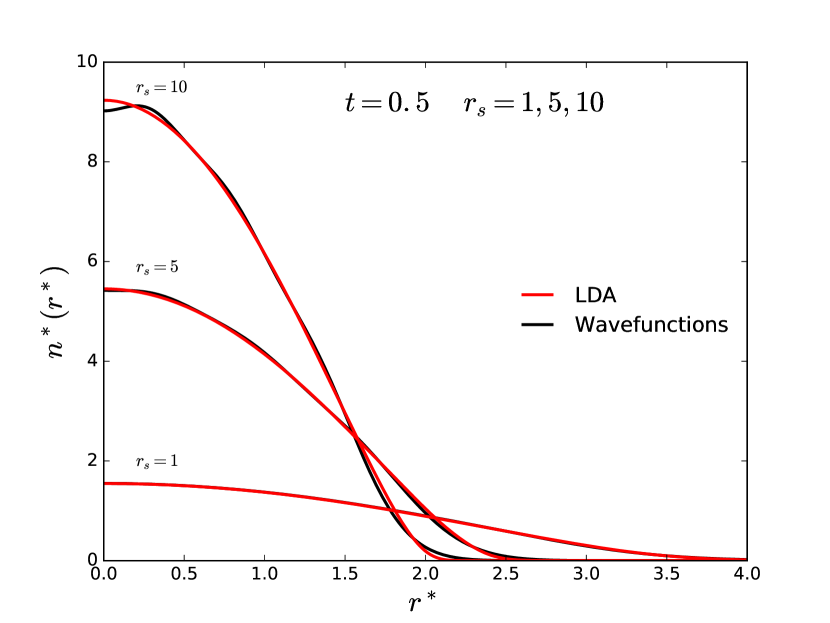
Figure 8: Comparison of density profiles calculated with Harmonic oscillator wavefunctions (black lines) and with the Thomas-Fermi approximation (red lines) for $t=0.5$ and $r_{s}=1,5,10$.

References

- (1) V. Karasiev, T. Sjostrom, D. Chakraborty, J. W. Dufty , F. E. Harris , K. Runge, and S. B. Trickey, Innovations in Finite-Temperature Density Functionals, Chapter in Computational Challenges in Warm Dense Matter, edited by F. Graziani et al. (Springer Verlag) in print; R.P. Drake,”High Energy Density Physics”, Phys. Today 63, 28-33 (2010) and refs. therein; Basic Research Needs for High Energy Density Laboratory Physics (Report of the Workshop on Research Needs, November 2009), U.S. Department of Energy, Office of Science and National Nuclear Security Administration, 2010, see Chapt. 6 and references therein.
- (2) F. Perrot and M. W. C. Dharma-wardana, Phys. Rev. B 62 16536 (2000); M. W. C. Dharma-wardana, Int. J. Quantum Chem. 112 53 (2012).
- (3) J. W. Dufty and S. Dutta, Contrib. Plasma Phys. 52 100 (2012); Phys. Rev. E 87 032101 (2013).
- (4) S. Dutta and J. Dufty, Phys. Rev. E 87, 032102 (2013).
- (5) S. Dutta and J. Dufty, Euro. Phys. Lett., 102 67005 (2013).
- (6) Y. Liu and J. Wu, J. Chem. Phys. 140, 084103 (2014).
- (7) E. Brown, B. Clark, J. DuBois, and D. Ceperley, Phys. Rev. Lett. 110 146405 (2013).
- (8) J. Lutsko, Recent Developments in Classical Density Functional Theory, Adv. Chem. Phys. 144, S. Rice, ed. (J. Wiley, Hoboken, NJ, 2010).
- (9) J-P Hansen and I. MacDonald, Theory of Simple Liquids, (Academic Press, London, 2006).
- (10) M. Allen and D. Tildesley, Computer simulation of liquids. Oxford University Press, NY, 1989)
- (11) J. Wrighton, J. W. Dufty, H. Kählert, and M. Bonitz, Phys. Rev. E 80, 066405 (2009); J. Wrighton, J. W. Dufty, M. Bonitz, and H. Kählert, Contrib. Plasma Phys. 50, 26 (2010).
- (12) J. Wrighton, J. W. Dufty, and S. Dutta, in Adv. Quant. Chem. 71 (Elsevier, NY, 2015).
- (13) M. Bonitz, C. Henning, and D. Block, Rep. Prog. Phys. 73, 0665(2010).
- (14) M. Bonitz, P. Ludwig, H. Baumgartner, C. Henning, A. Filinov, D. Block, O. Arp, A. Piel, S. Käding, Y. Ivanov, A. Melzer, H. Fehske, and V. Filinov Phys. Plasmas 15, 055704 2008.
- (15) P. Attard, J. Chem. Phys. 91, 3072 (1989).
- (16) J. Wrighton, H. Kählert, T. Ott, P. Ludwig, H. Thomsen, J. Dufty, and M. Bonitz, Contrib. Plasma Phys. 52, 45 (2012).
- (17) F. Perrot, Phys. Rev. A 20, 586 (1979).
- (18) C. Amovilli and N. March, Phys. Rev. B 76, 195104 (2007).
- (19) G. Kelbg, Ann. Phys., 467, 219 (1963).
- (20) A. Filinov, V. Golubnychiy, M. Bonitz, W. Ebeling, and J. Dufty, Phys. Rev. E 70, 046411 (2004).
- (21) D. Dubin and T. O’Neill, Rev. Mod. Phys. 71, 87 (1999).
- (22) C. R. McDonald, G. Orlando, J.W. Abraham, D. Hochstuhl, M. Bonitz, and T. Brabec, Phys. Rev. Lett. 111, 256801 (2013).
- (23) A. Melzer and D. Block in Introduction to Complex Plasmas, M. Bonitz, H. Horing, and P. Ludwig, eds. (Springer-Verlag, NY, 2010).
- (24) S. M. Reimann and M. Manninen, Rev. Mod. Phys. 74, 1283 (2002).