Distribution of the k^th smallest Dirac operator eigenvalue : an update

Abstract:

Based on the exact relationship to random matrix theory, we present an alternative method of evaluating the probability distribution of the $k^{\rm th}$ smallest Dirac eigenvalue in the $\varepsilon$-regime of QCD and QCD-like theories. By utilizing the Nyström-type discretization of Fredholm determinants and Pfaffians, practical trouble of evaluating multiple integrations is circumvented and technical restrictions on the parities of the number of flavors and of the topological charge present in our previous treatment for $\beta=1$ and 4 cases [Phys. Rev. D63, 045012 (2001)] are partly lifted. This method is also applied to the distributions of spacings between $k^{\rm th}$ nearest-neighboring levels in the mobility edges of Anderson Hamiltonian and Dirac operator in high-temperature QCD.

1 Introduction

Random matrix theory opened a nonperturbative and analytical window into the physics of chiral symmetry breaking in QCD [1]. Namely, chiral Gaussian ensemble of Hermitian random matrices of the block off-diagonal form $H=\left({\ 0\ \ W\atop W^{\dagger}\;0}\right)$ with $W\in\mathbb{R}^{N\times(N+\nu)}$, $\mathbb{C}^{N\times(N+\nu)}$, or $\mathbb{H}^{N\times(N+\nu)}$ (labeled by the Dyson indices $\beta=1,2,4$, respectively), that are distributed according to the unnormalized probability measure

$$dW\,{\rm e}^{-\beta{\rm tr}\,W^{\dagger}W}\prod_{f=1}^{n}\mathrm{det}\left(\begin{matrix}m_{f}&iW\\ iW^{\dagger}&m_{f}\end{matrix}\right),$$ (1)

($\det\to{\rm qdet}$ for $\beta=4$) exhibits the spontaneous symmetry breaking pattern expected for confining gauge theories coupled to $n$ flavors of Dirac ($\beta=1,2$) or Majorana ($\beta=4$) fermions in a pseudoreal, complex, or real representation, in a sector of topological charge $\nu$ [2]. The joint distribution of the square of $N$ positive eigenvalues of $H$ (singular values of $W$) $\{x_{i}\}$ then reads

$$P(\{x\})=\mathcal{Z}_{\nu}(\{m\})^{-1}\prod_{i=1}^{N}\Bigl{(}x_{i}^{\beta(\nu+1)/2-1}{\rm e}^{-\beta x_{i}}\prod_{f=1}^{n}(x_{i}+m_{f}^{2})\Bigr{)}\prod_{j>k}^{N}|x_{j}-x_{k}|^{\beta}.$$ (2)

The universal $k$-level correlation functions $R_{k}$ (including the spectral density $\rho(\zeta)$ for $k=1$) of these ‘massive’ ensembles, expressed as determinantal/Pfaffian point processes [3, 4], are not the quantities that most suit to fit the Dirac spectral data from lattice QCD simulations, as the amplitude of oscillation of $R_{k}$ quickly decreases for a large separation between eigenvalues or from the origin. Instead, the clear winner is the individual distributions $p_{k}(\zeta)$ of each ordered eigenvalues (Fig. 1), which are also universal [5]. Each of them has a characteristic, quasi-Gaussian peaky form that resolves the spectral density (the latter is almost structureless for $\zeta\gg 1$) as $\rho(\zeta)=\sum_{k\geq 1}p_{k}(\zeta)$.

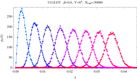
Figure 1: Eight smallest EV distributions of chGUE ($\beta=2$), $n=\nu=0$ fitted to the Dirac spectrum of compact U(1) LGT [left]. Combining 8 values of the mean level spacing $\Delta$ obtained by fitting each distribution, the quenched chiral condensate $\Sigma={\pi}/{V\Delta}$ is determined as precisely as $\Sigma a^{3}=0.51025(10)$. This precision cannot be hoped for from fitting the spectral density or any single individual EV distribution [right].

Among established techniques of computing so-called gap probabilities, neither the construction of Fredholm eigenfunctions/eigenvalues a la Gaudin-Mehta [6], of linear differential equations a la Edelman [7], or of Painlevé transcendental equations a la Tracy-Widom [8] (in historical order) is promising for the individual distribution of the $k^{\mathrm{th}}$ smallest eigenvalue of the massive chiral ensemble (1). Extending Forrester-Hughes’ work [9], we thus proposed an alternative method [10] consisting of 3 steps: (i) relate the joint distribution of the first $k$ eigenvalues, $\frac{1}{(N-k)!}\int_{x_{k}}^{\infty}dx_{k+1}\cdots\int_{x_{k}}^{\infty}dx_{N}\,P(\{x\})$, to the normalization (partition function) $\mathcal{Z}$ with $\beta k+\beta(\nu+1)/2-1$ additional masses and a fixed topological charge $2/\beta+1$, by a shift of all variables by $x_{k}$, (ii) replace $\mathcal{Z}$’s by their microscopically-scaled forms [11, 4] as functions of scaled variables $\zeta_{i}=\sqrt{8Nx_{i}}$ and $\mu_{f}=\sqrt{8N}m_{f}$, and (iii) integrate over the variables $\zeta_{1},\ldots,\zeta_{k-1}$ in a cell $0\leq\zeta_{1}\leq\cdots\leq\zeta_{k-1}\leq\zeta_{k}$. This simple procedure leads to compact expressions for some easy cases, such as $\beta=2,n=0,k=1$ for which $p_{1}(\zeta)=(\zeta/2){\rm e}^{-\zeta^{2}/4}\det[I_{f-g+2}(\zeta)]_{f,g=1}^{\nu}$ [9]. However, the first and second steps entail restrictions to massive Dirac fermions and on the parity of the number of massless fermions ($\beta=4$) or of the topological charge ($\beta=1$), and the $(k-1)$-fold numerical integration in the third step becomes exponentially resource-consuming as $k$ increases. In this report we show that these technical problems can be partly circumvented by utilizing the quadrature method applied to Fredholm determinants [13].

2 Individual eigenvalue distribution

Consider a stochastic distribution of $N$ points $\{x_{1},\ldots,x_{N}\}$ on a real line. Let $E_{k}(J)$ denote the probability of finding exactly $k$ points from in a (joint of) interval(s) $J$. Then their generating function $E({z};J)$ is related to the $p$-point correlation functions of the densities $R_{p}(x_{1},\ldots,x_{p}):=\left\langle\prod_{k=1}^{p}\rho(x_{k})\right\rangle$, $\rho(x):=\sum_{i=1}^{N}\delta(x-x_{i})$, by

$$E({z};J):=\sum_{k\geq 0}(1-{z})^{k}E_{k}(J)=1+\sum_{p\geq 1}\frac{(-{z})^{p}}{p!}\int_{J}dx_{1}\cdots\int_{J}dx_{p}\,R_{p}(x_{1},\ldots,x_{p}).$$ (3)

Eigenvalues of a unitary ensemble ($\beta=2$) obey a determinantal point process, i. e. their $p$-point correlation function is written as a $p\times p$ determinant of a scalar kernel $K(x,x^{\prime})$ constructed from orthonormal functions $\psi_{i}(x)$ corresponding to the weight in (2),

$$R_{p}(x_{1},\ldots,x_{p})=\det[K(x_{i},x_{j})]_{i,j=1}^{p},\ \ \ K(x,x^{\prime}):=\sum_{i=1}^{N}\psi_{i}(x)\psi_{i}(x^{\prime}).$$ (4)

Likewise, eigenvalues of an orthogonal ensemble ($\beta=1$), a symplectic ensemble ($\beta=4$), or ensembles interpolating two different classes (Dyson’s Brownian motion model) obey a Pfaffian point process, i. e. their $p$-level correlation function is written as a $p\times p$ quaternion determinant of a quaternionic kernel $\boldsymbol{K}(x,x^{\prime})$ or a $2p\times 2p$ Pfaffian of its $\mathbb{C}$-number $2\times 2$-matrix representative (denoted by the same $\boldsymbol{K}(x,x^{\prime})$ for notational simplicity),

$$R_{p}(x_{1},\ldots,x_{p})={\rm qdet}[\boldsymbol{K}(x_{i},x_{j})]_{i,j=1}^{p}={\rm Pf}\,Z[\boldsymbol{K}(x_{i},x_{j})]_{i,j=1}^{p},$$ (5)

($Z=i\sigma_{2}\oplus\cdots\oplus i\sigma_{2}$ denotes a skew-unit matrix), constructed from skew-orthonormal functions. Due to these determinantal properties (4), (5) and the identity (3), the generating function $E({z};J)$ is expressed as a Fredholm (quaternion-)determinant

$$E({z};J)={\rm det}({\mathbb{I}}-{z}\hat{K}_{J})\ \mbox{(scalar)}\ \ \mbox{or}\ \ {\rm qdet}({\mathbb{I}}-{z}\hat{\boldsymbol{K}}_{J})\ \mbox{(quaternion)},$$ (6)

where $\hat{K}_{J}$ and $\hat{\boldsymbol{K}}_{J}$ denote integral operators acting on the Hilbert spaces of 1- and 2-component $\mathcal{L}^{2}$ functions on $J$ with involution kernels $K(x,x^{\prime})$ and $\boldsymbol{K}(x,x^{\prime})$, respectively. From (3), (6), and the relationship between a Pfaffian and a determinant ${\rm Pf}={\rm det}^{1/2}$, $E_{k}(J)$ is expressed as

$$E_{k}(J)=\frac{1}{k!}\left(-\partial_{z}\right)^{k}\left.{\rm det}({\mathbb{I}}-{z}\hat{K}_{J})\right|_{{z}=1}\ \mbox{(scalar)}\ \ \mbox{or}\ \ \frac{1}{k!}\left(-\partial_{z}\right)^{k}\left.{\rm det}({\mathbb{I}}-{z}\hat{\boldsymbol{K}}_{J})^{1/2}\right|_{{z}=1}\ \mbox{(quaternion)}.$$ (7)

Now we set $J=[0,s]$ and abbreviate $\hat{K}_{s}:=\hat{K}_{[0,s]}$, $E_{k}(s):=E_{k}([0,s])$, etc. By performing ${z}$-derivatives explicitly, $E_{k}(s)$ are expressed by Fredholm determinants at ${z}=1$ and the functional traces of the resolvents $T_{n}(s)={\rm tr}\bigl{(}\hat{{K}}_{s}({\mathbb{I}}-\hat{{K}}_{s})^{-1}\bigr{)}^{n}\ \mbox{(scalar)}$ or ${\rm tr}\bigl{(}\hat{\boldsymbol{K}}_{s}({\mathbb{I}}-\hat{\boldsymbol{K}}_{s})^{-1}\bigr{)}^{n}/2\ \mbox{(quaternion)}$ as

$$E_{0}(s)=\det({\mathbb{I}}-\hat{K}_{s})\ \ \mbox{(scalar)}\ \ \mbox{or}\ \ \det({\mathbb{I}}-\hat{\boldsymbol{K}}_{s})^{1/2}\ \ \mbox{(quaternion)},$$ (8)

$$E_{1}(s)=E_{0}(s)T_{1},\quad E_{2}(s)=\frac{E_{0}(s)}{2!}\left(T_{1}^{2}-T_{2}\right),\quad E_{3}(s)=\frac{E_{0}(s)}{3!}\left(T_{1}^{3}-3T_{1}T_{2}+2T_{3}\right),$$

$$E_{4}(s)=\frac{E_{0}(s)}{4!}\left(T_{1}^{4}-6T_{1}^{2}T_{2}+3T_{2}^{2}+8T_{1}T_{3}-6T_{4}\right),$$

$$E_{5}(s)=\frac{E_{0}(s)}{5!}\left(T_{1}^{5}-10T_{1}^{3}T_{2}+20T_{1}^{2}T_{3}+15T_{1}T_{2}^{2}-30T_{1}T_{4}-20T_{2}T_{3}+24T_{5}\right),$$

$$E_{6}(s)=\frac{E_{0}(s)}{6!}\left\{{{T_{1}^{6}-15T_{1}^{4}T_{2}+40T_{1}^{3}T_{3}+45T_{1}^{2}T_{2}^{2}-90T_{1}^{2}T_{4}-120T_{1}T_{2}T_{3}}\atop{-15T_{2}^{3}+144T_{1}T_{5}+90T_{2}T_{4}+40T_{3}^{2}-120T_{6}}}\right\},$$

$$E_{7}(s)=\frac{E_{0}(s)}{7!}\left\{{{T_{1}^{7}-21T_{1}^{5}T_{2}+70T_{1}^{4}T_{3}+105T_{1}^{3}T_{2}^{2}-210T_{1}^{3}T_{4}-420T_{1}^{2}T_{2}T_{3}-105T_{1}T_{2}^{3}+504T_{1}^{2}}\atop{\times T_{5}+630T_{1}T_{2}T_{4}+280T_{1}T_{3}^{2}+210T_{2}^{2}T_{3}-840T_{1}T_{6}-504T_{2}T_{5}-420T_{3}T_{4}+720T_{7}}}\right\}.$$

Then the individual distribution $p_{k}(s)$ of the $k^{\rm th}$ smallest positive eigenvalue is expressed in terms of $E_{0}(s),\ldots,E_{k-1}(s)$ as $p_{k}(s)=-\partial_{s}\sum_{\ell=0}^{k-1}E_{\ell}(s).$

An efficient way of numerically evaluating the Fredholm determinant of a trace-class operator $\hat{{K}}_{s}$ or $\hat{\boldsymbol{K}}_{s}$ is the Nyström-type discretization [13]

$${\rm det}({\mathbb{I}}-\hat{{K}}_{s})\simeq\det\left[\delta_{ij}-K(x_{i},x_{j})\sqrt{w_{i}\,w_{j}}\right]_{i,j=1}^{m},\ \ {\rm det}({\mathbb{I}}-\hat{\boldsymbol{K}}_{s})\simeq\det\left[I\delta_{ij}-\boldsymbol{K}(x_{i},x_{j})\sqrt{w_{i}\,w_{j}}\right]_{i,j=1}^{m}.$$ (9)

Here we employ a quadrature rule consisting of a set of points $\{x_{i}\}$ taken from the interval $[0,s]$ and associated weights $\{w_{i}\}$ such that ${\int_{0}^{s}f(x)dx\simeq\sum_{i=1}^{m}f(x_{i})w_{i}}$. Similarly the functional trace in $T_{n}(s)$ can be approximated by its discretized version. For a practical purpose we choose the Gauss-Legendre quadrature rule, i.e. sampling $\{x_{i}\}$ from the nodes of Legendre polynomials normalized to $[0,s]$, so that the discretization gives an exact value for an arbitrary $(m-1)^{\rm th}$-order polynomial $f(x)$. Exponential convergence in $m$ to the exact value of the Fredholm determinant is guaranteed for any smooth kernel. This method was previously applied to the quenched ($n=0$) chiral ensemble interpolating chGSE and chGUE, which enabled precise determination of the pion decay constant in the SU(2) gauge theory [16]. There we found it far more than sufficient to set the approximation order $m$ to be $\lesssim 100$ for the purpose of fitting the lattice Dirac spectra.

3 Chiral ensembles

The scalar kernel describing the eigenvalue correlation of the chiral GUE ($\beta=2$) in the microscopic scaling limit is given in Eq.(33) of Ref.[3]. As an illustrative example that is applicable for QCD with light flavors, we exhibit $p_{1\sim 8}(\zeta)$ with $n=2+1$ (Fig. 2), computed by Nyström-type discretization of the Fredholm determinant and traces (8) of the kernel in the confluent limit,

$$K(\zeta,\zeta^{\prime};\mu,\mu,\mu^{\prime})=\frac{\sqrt{\zeta\zeta^{\prime}}}{(\zeta^{\prime}{}^{2}-\zeta^{2})(\zeta^{2}+\mu^{2})(\zeta^{\prime}{}^{2}+\mu^{2})\sqrt{(\zeta^{2}+\mu^{\prime}{}^{2})(\zeta^{\prime}{}^{2}+\mu^{\prime}{}^{2})}}\frac{\det{B}(\zeta,\zeta^{\prime};\{\mu\})}{\det{A}(\{\mu\})},$$

$$A=\left[\begin{array}[]{c}(-\mu)^{g-1}I_{\nu+g-1}(\mu)\\ (-\mu)^{g-2}I_{\nu+g-2}(\mu)\\ (-\mu^{\prime})^{g-1}I_{\nu+g-1}(\mu^{\prime})\end{array}\right]_{g=1,2,3},\ \ B={\small\left[\begin{array}[]{c}\zeta^{g-1}J_{\nu+g-1}(\zeta)\\ \zeta^{\prime}{}^{g-1}J_{\nu+g-1}(\zeta^{\prime})\\ (-\mu)^{g-1}I_{\nu+g-1}(\mu)\\ (-\mu)^{g-2}I_{\nu+g-2}(\mu)\\ (-\mu^{\prime})^{g-1}I_{\nu+g-1}(\mu^{\prime})\end{array}\right]_{g=1,\ldots,5}.}$$ (18)

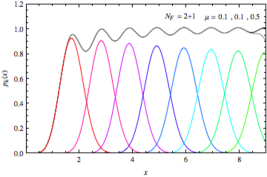
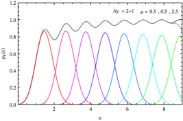
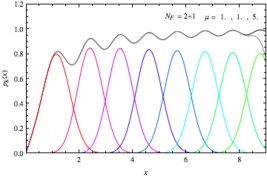
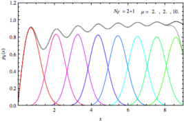
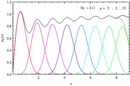
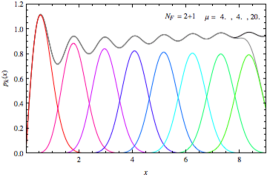
Figure 2: 8 smallest EV distributions of massive chGUE, $n=2+1,\nu=0$, with $\pi\mu=\pi\mu^{\prime}/5=0.1\sim 4.0$.

Note that the scalar kernel (4) in the scaling limit is a self-convolution of functions $V(t,\zeta)$ which originate from the orthonormal functions $\psi_{i}(x)$ with $t=i/N$ and $\zeta=\sqrt{8Nx}$ ($\{\mu\}$ is suppressed),

$$K(\zeta,\zeta^{\prime})=\int_{0}^{1}dt\,V(t,\zeta)V(t,\zeta^{\prime})=({V}^{T}\circ{V})(\zeta,\zeta^{\prime}),\ \ \ \ \int_{0}^{\infty}d\zeta\,V(t,\zeta)V(t^{\prime},\zeta)=\delta(t-t^{\prime})$$

$$V(t,\zeta)=\frac{\sqrt{\zeta/2}}{\prod_{f=1}^{n}\sqrt{\zeta^{2}+\mu^{2}_{f}}}\frac{\det{\tilde{B}}(t;\zeta)}{\det{\tilde{A}}(t)},$$ (19)

$$\tilde{A}=\left[(-\mu_{f})^{g-1}I_{\nu+g-1}(\sqrt{t}\mu_{f})\right]_{f,g=1}^{n},\ \ \tilde{B}=\left[\begin{array}[]{c}\zeta^{g-1}J_{\nu+g-1}(\sqrt{t}\zeta)\\ \left[(-\mu_{f})^{g-1}I_{\nu+g-1}(\sqrt{t}\mu_{f})\right]_{f=1}^{n}\end{array}\right]_{g=1}^{n+1}.$$ (22)

Thus its Fredholm determinant factorizes into the product of two Fredholm determinants [14],

$$E(z;[0,s])={\rm det}({\mathbb{I}}+\sqrt{z}\hat{V}_{s}){\rm det}({\mathbb{I}}-\sqrt{z}\hat{V}_{s}),$$ (23)

where $\hat{V}_{s}$ is an integral operator $\mathcal{L}^{2}[0,1]\to\mathcal{L}^{2}[0,1]$ (the domain of definition is rescaled from $[0,s]$) of convolution by a rescaled kernel $\sqrt{s}V(t,s\zeta)$. Numerical evaluation of (23) gives an alternative, convenient way of computing $p_{k}(s)$ of chiral GUE.

In the case of chiral GSE ($\beta=4$), the partition function and correlation functions, from which the quaternion kernel can easily read off, have readily been worked out in Refs. [4]. Thus one can simply apply the quaternion side of (9) to compute $p_{k}(\zeta)$. However, we must admit that the case of chiral GOE ($\beta=1$) at even $\nu$, which lay outside of the scope of Ref.[10], still poses a problem; it is because the exponential convergence of the quadrature approximation is not guaranteed for its quaternion kernel which includes a discontinuous signature function.

4 q-Hermite ensemble

Among the random matrix ensembles that possess weak confining potentials ($\sim{\rm tr}(\log H)^{2}$) and break the Wigner-Dyson universality, the so-called $q^{-1}$-Hermite ensemble [17] associated with the Askey weight leads to a translationally invariant spectrum in the bulk and serves as a candidate of a phenomenological model describing the mobility edge of disordered Hamiltonians. As $q$ is deformed from unity, its kernel in far away from the origin,

$$K_{q}(\zeta,\zeta^{\prime})=\frac{a\vartheta_{1}(\pi(\zeta-\zeta^{\prime}),q)}{\pi\vartheta_{1}^{\prime}(0,q)\sinh(a(\zeta-\zeta^{\prime}))},\ \ q:={\rm e}^{-{\pi^{2}}/{a}},$$ (24)

interpolates between Wigner and Poisson statistics without crystallization of eigenvalues as seen in other ensembles [18]. Here we slightly extend our previous observation that by tuning a single parameter $q$, the level spacing distribution of this deformed ensemble can perfectly fit the scale-invariant critical statistics of the mobility edge of Anderson Hamiltonians [19], by considering the distribution of spacings between $k^{\rm th}$ nearest-neighboring levels, $p_{k}(s)$. This quantity is related to the gap probabilities $E_{\ell}([-s/2,s/2])$ as $p_{k}(s)=\partial_{s}^{2}\sum_{\ell=0}^{k-1}E_{\ell}([-s/2,s/2])$, which we evaluate by the quadrature approximation of the Fredholm determinant and traces of the elliptic kernel (24).

In Fig.3 we performed one-parameter fitting of $p_{k}(s)$ to the spacing data from the mobility edges (their locations are known from previous studies) of the Anderson Hamiltonian in the unitary class and the stagger Dirac operator of high-temperature QCD [20]. Impressive fittings especially in the case of Anderson Hamiltonian again recalls us the power of combining the information from multiple level spacing distributions; if applied to the QCD data on larger lattices, it should help identifying the location of the mobility edge and the critical parameter in high precision.

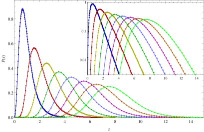
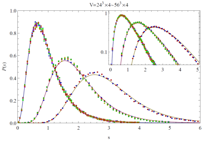
Figure 3: Distributions of spacings between $k^{\rm th}$ nearest-neighboring levels $p_{k}(s)$, $k=1,\ldots,8$ of the $q^{-1}$-Hermite ensemble fitted to the mobility edges of unitary Anderson Hamiltonian on $V=20^{3}$ [left] and of high-temperature QCD Dirac operator $(T=2.6T_{c})$ on $V=(24^{3}\sim 56^{3})\times 4$ (eigenvalue data provided by T. Kovács) [right]. Parameters and lattice settings are the same as in Figs.2 and 6 of Ref.[20].