Generalised block bootstrap and its use in meteorology

Abstract

In an earlier paper Rakonczai et al. (2014), we have emphasized the effective sample size for autocorrelated data. The simulations were based on the block bootstrap methodology. However, the discreteness of the usual block size did not allow for exact calculations. In this paper we propose a generalisation of the block bootstrap methodology, relate it to the existing optimisation procedures and apply it to a temperature data set. Our other focus is on statistical tests, where quite often the actual sample size plays an important role, even in case of relatively large samples. This is especially the case for copulas. These are used for investigating the dependencies among data sets. As in quite a few real applications the time dependence cannot be neglected, we investigated the effect of this phenomenon to the used test statistic. The critical values can be computed by the proposed new block bootstrap simulation, where the block sizes are determined e.g. by fitting a VAR model to the observations. The results are illustrated for models of the used temperature data.
Keywords: block bootstrap, copula, temperature data, test of homogeneity, VAR models

1 Introduction

In the last decades the bootstrap methodology has become more and more widespread in different areas of statistical applications. See e.g. Chernick (2011) for a review of possible areas from spatial models to financial data and data mining, where bootstrap may be used. In this paper we focus on the effect of the serial dependence, naturally arising in many time series data. The bootstrap samples must match the dependence within the data, so the block bootstrap is the suggested method for bootstrapping time series. Hall et al. (1995) investigate this approach in some detail, including suggestions for selecting the optimal block size. In an earlier paper Rakonczai et al. (2014), we investigated the possibilities for using the block bootstrap methods for checking the validity of the copula models. In this paper we present an improvement to the classical block bootstrap methodology, which is especially relevant in our applications.

In Section 2, we first briefly review the elements of stationary time series. In the bivariate case, the vector autoregression (VAR) process is one of the most important models, becoming popular first in the area of econometrics (Sims (1980)). For recent applications of VAR models in meteorology, see for example Hill et al. (2014), Norrulashikin et al. (2015) or Farook and Kannan (2016). We briefly present the main properties of VAR models, which are used in the sequel and present the notations.

In Section 3, we introduce the concept of copulas, the most convenient objects for analysing the dependence structures among variables. Their history goes as back as Hoeffding (1940), but their applications are much more recent. However, they have spread very quickly to the most important areas – for a recent analysis in meteorology, see Cong and Brady (2012). Most of these works use different parametric copula models, but we are more interested in testing for possible changes in the dependency structure of our temperature data, so also introduce the most recent approaches in testing homogeneity of such models, which are based on the empirical copula process.

Section 4 is devoted to the bootstrap resampling method, including the block bootstrap approach, which is suitable for the case of serial dependent observations. Here we introduce a generalisation, which helps overcoming the problem that originally the block size was supposed to be a natural number. In our approach the block size is a random variable, but it contains the original block bootstrap as a special case. Due to this small variance in the sample size, it overcomes the problem of extensive random error in case of the so-called stationary bootstrap (Politis and Romano (1994)).

In Section 5 we apply our approach to the gridded temperature data base of E-OBS, which is a product of the EU-FP6 project ENSEMBLES (Haylock et al. (2008)). Here we use the daily mean temperature data from the 0.5 grade-grid. Our focus is on checking for possible changes in the dependence pattern between the grid point of Budapest and some other grid points within the Carpathian Basin. We show that in some cases there is a significant deviation from homogeneity of the first and second part of the data. The conclusion summarizes our findings and gives some interesting open questions.

2 Vector autoregression (VAR) processes

We call the $d$-dimensional series $\{\mathbf{X}_{t}\}_{t\in\mathbb{Z}}=(\mathbf{X}_{0},\mathbf{X}_{\pm 1},\mathbf{X}_{\pm 2},\ldots)$ a time series if its elements are $d$-dimensional random vectors, which are usually not independent from each other. Here we consider $t$ as the time. Let us assume that the random variables have finite second moments. The time series $\{\mathbf{X}_{t}\}_{t\in\mathbb{Z}}$ is weakly stationary (later we just call it stationary), if for all $t$, if neither the mean function $E(\mathbf{X}_{t})$ nor the covariance matrix Cov$(\mathbf{X}_{t+s},\mathbf{X}_{t})$ depends on $t$ for all $s\in\mathbb{Z}$. Stationarity is an important property, it means that the time series is translation invariant.

One of the most frequently applied time series models are the so-called autoregressive (AR) processes and their multidimensional counterparts, the vector-autoregressive (VAR) models. In the following, we define the VAR($p$) process and give its main properties in two dimensions as this is necessary to our applications.

The time series $\{\mathbf{X}_{t}\}_{t\in\mathbb{Z}}=\{(X_{1,t},X_{2,t})^{T}\}_{t\in\mathbb{Z}}$ is called a zero-mean two-dimensional VAR($p$) process if

$$\mathbf{X}_{t}=A_{1}\mathbf{X}_{t-1}+A_{2}\mathbf{X}_{t-2}+\ldots+A_{p}\mathbf{X}_{t-p}+\bm{\varepsilon}_{t},$$ (1)

where $A_{1},\ldots,A_{p}$ are $2\times 2$ parameter matrices and the $\{\bm{\varepsilon}_{t}\}_{t\in\mathbb{Z}}$ independent innovation process is a two-dimensional white noise with $E(\bm{\varepsilon}_{t})=\mathbf{0}=(0,0)^{T}$ and Cov$(\bm{\varepsilon}_{t})=C$ symmetric positive definite covariance matrix. The VAR($p$) process is stationary if the roots of the $P(x)=\det(I_{2}-A_{1}x-\ldots-A_{p}x^{p})$ characteristic polynomial lie outside the unit circle.

Any VAR($p$) process can be rewritten as a VAR(1) process in the following way: $\mathbf{Y}_{t}=A\mathbf{Y}_{t-1}+\mathbf{e}_{t}$, where
$\mathbf{Y}_{t}=\begin{pmatrix}\mathbf{X}_{t}\\ \mathbf{X}_{t-1}\\ \vdots\\ \mathbf{X}_{t-p+1}\end{pmatrix}$, $\mathbf{e}_{t}=\begin{pmatrix}\bm{\varepsilon}_{t}\\ \mathbf{0}\\ \vdots\\ \mathbf{0}\end{pmatrix}$ and $A=\begin{pmatrix}A_{1}&A_{2}&\cdots&A_{p-1}&A_{p}\\ I_{2}&\mathbf{0}&\cdots&\mathbf{0}&\mathbf{0}\\ \mathbf{0}&I_{2}&\cdots&\mathbf{0}&\mathbf{0}\\ \vdots&\vdots&\ddots&\vdots&\vdots\\ \mathbf{0}&\mathbf{0}&\ldots&I_{2}&\mathbf{0}\end{pmatrix}$. This representation is more convenient in calculating the autocovariances. An equivalent condition for stationarity is that all the eigenvalues of the coefficent matrix $A$ are smaller than one in modulus. In this case the time series is causal – it has an infinite moving average representation in the form $\mathbf{Y}_{t}=\sum\limits_{i=0}^{\infty}A^{i}\mathbf{e}_{t-i}$.

For the remainder of this section we assume that $\mathbf{X}_{t}$ is stationary. Let us denote with $\Gamma_{X}(h)=E(\mathbf{X}_{1+h}\mathbf{X}_{1}^{T})$ the autocovariance function of the process $\mathbf{X}_{t}$. $\Gamma_{X}(h)$ is a $2\times 2$ matrix valued function, the symbols $\gamma_{i,j}(h)$ stand for its elements. We denote with $\Gamma_{Y}(h)=E(\mathbf{Y}_{1+h}\mathbf{Y}_{1}^{T})$ the $2p\times 2p$ matrix valued autocovariance function of the process $\mathbf{Y}_{t}$. The covariance matrix of $\mathbf{Y}_{t}$ is $\Gamma_{Y}(0)$ which can be determined by solving the matrix equation $\Gamma_{Y}(0)-A\,\Gamma_{Y}(0)A^{T}=\text{Cov}(\mathbf{e_{t}})$. It is easy to see that for $1\leq h\in\mathbb{Z}$, the autocovariances can be calculated by $\Gamma_{Y}(h)=A^{h}\Gamma_{Y}(0)$. The powers of the matrix $A$ can easily be computed using the spectral decomposition. Lastly, we need the autocovariance matrix of the original process, and by the construction, it is the upper left $2\times 2$ submatrix of $\Gamma_{Y}(h)$.

In the applications we will use the covariance matrix of the sample mean. The following asymptotic result will be crucial in our investigations: if $\sum\limits_{h=-\infty}^{\infty}|\gamma_{i,i}(h)|<\infty$ for $i=1,2$, then

$$n\cdot\text{tr}\left(\text{Cov}(\overline{\mathbf{X}}_{n})\right)\underset{}{\longrightarrow}\sum\limits_{i=1}^{2}\sum\limits_{h=-\infty}^{\infty}\gamma_{i,i}(h)\ \ \ \ \text{as }n\to\infty,$$ (2)

where tr$(\cdot)$ denotes the trace of a matrix.

It is important to check if the chosen time series model is adequate. If the model fits well, the fitted residuals should behave as a realisation of a white noise process. The hard part is to check whether the residuals are independent, thus there is no serial dependence. There are several methods for verifying this problem, the most standard is the Ljung-Box test, which tests whether a specified group (usually the first 10-20 lags) of autocorrelations is different from zero. Another often applied serial correlation test is the Breusch-Godfrey test. A more recent multidimensional approach was published in the paper Kojadinovic and Yan (2011), where the test was based on the empirical copula process. The main ideas and the concept of this test stems from Genest and Rémillard (2004).

For further details about time series see for example Brockwell and Davis (2013) or Shumway and Stoffer (2011).

3 Copulas and their goodness-of-fit

Let $\mathbf{X}=(X_{1},\ldots,X_{d})^{T}$ be a random vector with joint distribution function $F_{\mathbf{X}}(\mathbf{x})=F_{X_{1},\ldots,X_{d}}(x_{1},\ldots,x_{d})$ and marginal distribution functions $F_{1}(x_{1})=F_{X_{1}}(x_{1}),$ $\ldots,F_{d}(x_{d})=F_{X_{d}}(x_{d})$. Sklar’s theorem claims that there exists a copula ${\bf C}$, a distribution over the $d$-dimensional unit cube, with uniform margins, such that

$$F_{X_{1},\ldots,X_{d}}(x_{1},\ldots,x_{d})={\bf C}\left(F_{1}(x_{1}),\ldots,F_{d}(x_{d})\right).$$

Moreover the copula $\mathbf{C}$ is unique if the marginal distribution functions are continuous. This construction allows the investigation of the dependence structure without specifying the marginal distributions. In the recent literature various families of copulas have been introduced, for an overview and examples see e.g. the introductory textbook of Nelsen (2007).

In this paper we focus on testing the homogeneity of copulas, motivated by the question whether the climate change has also an effect on the dependence between pairs of observations. If this change is indeed observable, then it may have a substantial effect on the spatial structure of temperature anomalies, worth for further meteorological investigations. So we do not have to go into the parametric inference, as we are just interested in the homogeneity analysis.

Let us suppose we have two independent samples of $\mathbb{R}^{d}$-valued vectors. The first sample is $\mathbf{X}_{1},\ldots,\mathbf{X}_{n}$ and the second one is $\mathbf{Y}_{1},\ldots,\mathbf{Y}_{m}$. Formally we intend to test the hypothesis that the dependence structure of the two copulas has arisen from the same copula $\mathbf{C}_{0}$. The most obvious way for testing the homogeneity of two copulas is to consider multidimensional $\chi^{2}$ approaches, but in this case we need to discretize the data, losing valuable information. In order to avoid its use, we can follow the approach of Rémillard and Scaillet (2009), who have developed a method for this problem. Their approach is based on the empirical copula, defined for the first sample as

$$\mathbf{C}_{1,n}(\mathbf{u})=\frac{1}{n}\sum_{i=1}^{n}I(\mathbf{U}_{i}\leq\mathbf{u}).$$

where $\mathbf{u}\in\mathbb{R}^{d}$ and $\mathbf{U}_{i}$ denotes the $d$-dimensional vector of the rank based pseudo-observations: $\mathbf{U}_{i}=\mathbf{U}_{i,n}=(U_{i1,n},\ldots,U_{id,n})$, where $n$ refers to the size of first sample and $U_{ij,n}=\frac{n}{n+1}F_{j}(X_{ij})$. For illustrations see Figure 1. Similarly, based on the pseudo-observations $\mathbf{V}_{i}$ of the second sample, we can define the empirical copula $\mathbf{C}_{2,m}(\mathbf{u})$.

Figure 1: Bivariate data and the corresponding pseudo-observations

The proposed tests for checking the homogeneity of two samples are based on functionals of the empirical process:

$$\kappa_{n,m}(t)=\frac{\mathbf{C}_{1,n}(t)-\mathbf{C}_{2,m}(t)}{\sqrt{\frac{1}{n}+\frac{1}{m}}},$$

where the asymptotic properties of the statistic can be based on the limit of the empirical copula processes. There are two different kind of approaches investigated in Genest et al. (2006): the Cramér-von Mises type statistic $S_{n,m}=\int\limits_{0}^{1}\left(\kappa_{n,m}(t)\right)^{2}dt$, and the Kolmogorov-Smirnov type statistic $T_{n,m}=\underset{0\leq t\leq 1}{\sup}\left|\kappa_{n,m}(t)\right|$. As the second approach is considered to be generally less powerful, we based our inference on the statistic $K_{*}=\frac{1}{N}\sum\limits_{t_{i}\in(0,1)}\left(\kappa_{n,m}(t_{i})\right)^{2}$, where $(t_{i})_{i=1}^{N}$ is an appropriately fine division of the interval $(0,1)$. After some calculations, the Cramér-von Mises test statistic can be written in the following form (see Rémillard and Scaillet (2009)):

$$S_{n,m}=\left(\frac{1}{n}+\frac{1}{m}\right)^{-1}\cdot \left[\frac{1}{n^{2}}\sum\limits_{i=1}^{n}\sum\limits_{j=1}^{m}\prod\limits_{s=1}^{d}(1-U_{is,n}\vee U_{js,n})+\right.$$ (3)

$$\hskip 8.53581pt+\frac{1}{m^{2}}\sum\limits_{i=1}^{m}\sum\limits_{j=1}^{m}\prod\limits_{s=1}^{d}(1-V_{is,m}\vee V_{js,m}-$$

$$\hskip 8.53581pt-\left.\frac{2}{nm}\sum\limits_{i=1}^{n}\sum\limits_{j=1}^{m}\prod\limits_{s=1}^{d}(1-(U_{is,n}\vee V_{js,m})\right],$$

where $u\vee v=\max(u,v)$.

As the limit distribution of the above statistic is not distribution-free, a simulation algorithm is needed to get critical values. The algorithm is the following:

1. Generate an $n$-element bootstrap sample from the first of the observation vectors – see its details in the next section –, and compute the statistic $S_{n,m}$, based on this and the original first sample;

2. Repeat the above steps as many times as needed to an accurate estimation of the $p$-values. The distribution function $G$ of the bootstrap statistic can be considered as a good approximation of the test statistic under $H_{0}$, so we used $1-G(S_{n,m})$ as the estimate of the $p$-value.

4 Bootstrap methods

The bootstrap is a usually computer-intensive, resampling method for estimating the distribution of a statistic of interest. The concept of the bootstrap was introduced in the classical article by Ben Efron (Efron (1979)) and since then, it has become one of the most widely used Monte Carlo methods in a number of aeras of applied sciences.

4.1 Bootstrap for i.i.d. data

Let $\mathcal{X}_{n}=(X_{1},\ldots,X_{n})^{T}$ be a sequence of independent, identically distributed (i.i.d.) random variables with unknown common univariate distribution $F$ and let $T_{n}=t_{n}(\mathcal{X}_{n};F)$ be a statistic (like the sample mean $\overline{X}$). Our main purpose is to approximate the unknown distribution of $T_{n}$ or its function of interest, for example its standard deviation (the standard error) or some quantiles.

The basic bootstrap method (mostly referred as i.i.d. bootstrap) is the following. For a given $\mathcal{X}_{n}$, we draw a random sample $\mathcal{X}_{m}^{*}=\{X_{1}^{*},\ldots,X_{m}^{*}\}$ of size $m$ (usually $m=n$) with replacement from $\mathcal{X}_{n}$. Therefore, the common distribution of the $X_{i}^{*}$’s is given by the empirical distribution $\hat{F}_{n}=n^{-1}\sum_{i=1}^{n}\delta_{X_{i}}$, where $\delta_{z}$ is the probability measure having unit mass at $z$. In the next step, we define the bootstrap version of the statistic $T_{n}$: $T_{m,n}^{*}=t_{m}(\mathcal{X}_{m}^{*};\hat{F}_{n})$. By repeating this procedure, we can approximate the unknown distribution $G_{n}$ by its bootstrap counterpart $G_{n}^{*}$. In most of the cases the distribution of $G_{n}^{*}$ cannot be determined explicitely, but it can be approximated by simulation.

4.2 Block bootstrap methods

In our case we are interested in the effect of serial dependence on the homogeneity tests and on modelling in general, for example on the covariance matrix of our estimators. If the data are dependent then the estimates based on i.i.d. bootstrap methods my not be consistent.

In the presence of serial dependence, one of the most commonly used methods is the so-called block bootstrap, see Lahiri (2003) for details. In this paper, we generalise the circular block bootstrap (CBB) which can be defined as follows. First, we wrap the data $X_{1},\ldots,X_{n}$ around a circle, i.e., define the series $Y_{t}=X_{t_{\rm{mod}(n)}}$ ($t\in\mathbb{N}$), where $\rm{mod}(n)$ denotes division "modulo $n$". This means that $X_{k}=Y_{k}=Y_{k+n}=Y_{2k+n}=\ldots$ for all $k\in\{1,2,\ldots,n\}$. For some $m$, let $i_{1},\ldots,i_{m}$ be a uniform sample from the set $\{1,2,\ldots,n\}$. Then, for a given block size $b$, we construct $n^{\prime}=m\cdot b$   ($n^{\prime}\approx n$) pseudo-data:

$Y^{*}_{(k-1)b+j}=Y_{i_{k}+j-1}$   where $j=1,\ldots,b$   and $k=1,\ldots,m$.

Finally, let us calculate the function of interest, for example the bootstrap sample mean as follows: $\overline{Y}^{*}_{n^{\prime}}=\frac{Y^{*}_{1}+\ldots+Y^{*}_{n^{\prime}}}{n^{\prime}}$.

Block length plays an important role in the process, and it is not trivial to determine its optimal value. Politis and White in their article Politis and White (2004) suggest an "automatic" block length selection algorithm (its correction was published in Patton et al. (2009)) - but the practical applications of this method are far from obvious as there are parameters in it, which have to be chosen.

We used a similar approach in our paper Rakonczai et al. (2014). Our idea was that we tried to find the best block size by fitting a model and then checking the variance of $\overline{X}$ with the help of the block bootstrap. The block size was determined as the $\widehat{b}$, for which the estimated trace of the covariance matrix was the nearest to the one got by the fitted VAR model:

$$\widehat{b}=\underset{1\leq b\,\in\mathbb{Z}}{\text{argmin}}\left|\text{tr}\left(\text{Cov}\left(\overline{X}_{\!V\!\!A\!R}\right)\right)-\text{tr}\left(\text{Cov}_{*}(\overline{X}_{b}^{*})\right)\right|,$$ (4)

where $\text{Cov}_{*}(\overline{X}_{b}^{*})=\text{Cov}(\overline{X}_{b}^{*}|\mathcal{X}_{n})$. In the literature, simulations are naturally based on integer block sizes. But using the block length of (4), the estimated trace of covariance may be not be close enough to the theoretical trace of covariance. The same is true for other methods for block size determination. This may cause substantial bias, as in our case the relative difference between subsequent values of tr$(\text{Cov}_{*}(\overline{X}_{b}^{*}))$ can be quite large, especially for small $b$. This can be overcome by the following generalisation of the block bootstrap methodology.

In case of $b\!>\!1$,  $b\!\in\!\mathbb{R}$, let the generalised block bootstrap sample be defined as follows. Let $k$ be a random integer between $1$ and the sample size $n$, and again, let us wrap the sample around the circle. The bootstrap blocks are either of length $\lfloor b\rfloor$ or $\lceil b\rceil$:
$X_{k},X_{k+1},\dots,X_{k+\lfloor b\rfloor}$ with probability $1-b+\lfloor b\rfloor$ $X_{k},X_{k+1},\dots,X_{k+\lceil b\rceil}$ with probability $b-\lfloor b\rfloor$
where $\lceil b\rceil$ denotes the upper, and $\lfloor b\rfloor$ the lower integer part of $b$. At last, we put the blocks together. This procedure ensures that for integer-valued $b$ the new definition coincides with the traditional one, so this is indeed a generalisation. In the applications (Section 5) we show the clear advantages of this approach. Actually all of the relevant algorithms for finding the optimal block size can easily be adapted to find a solution in this generalised sense. In our case, instead of (4), we simply solve the equation

$$\text{tr}\left(\text{Cov}(\overline{X}_{\!V\!\!A\!R})\right)=\text{tr}\left(\text{Cov}_{*}(\overline{X}_{b}^{*})\right).$$ (5)

In the same way as the circular block bootstrap sample, our generalized bootstrap sample is not a stationary process, conditional on the original sample. The block bootstrap sample is in only one case conditionally stationary: when the block lengths follow a geometric distribution, independent from each other (Politis and Romano (1994)).

The covariance matrix $\text{Cov}_{*}(\overline{X}_{b}^{*})$ can be explicitly calculated. Let us denote with $L_{1},L_{2},\ldots$ the block sizes – they are random variables independent from each other with common conditional distribution $P_{*}(L_{1}=\lceil b\rceil)=1-P_{*}(L_{1}=\lfloor b\rfloor)=b-\lfloor b\rfloor$. We can also write $L_{i}=\lfloor b\rfloor+J_{i}$, where $J_{i}|\mathcal{X}_{n}$ follows a Bernoulli distribution with parameter $p=b-\lfloor b\rfloor$. Let $N$ be the random variable, which gives the number of blocks with block size $\lfloor b\rfloor$. If we have $N$, we can calculate the number of blocks with block size $\lceil b\rceil$, we denote it with $g(N)$. So $g(N)=\left\lfloor\frac{n-N\cdot\lfloor b\rfloor}{\lceil b\rceil}\right\rfloor$. Let us denote the remainder block size with $r(N)$, we can calculate it from the others: $r(N)=n-N\cdot\lfloor b\rfloor-g(N)\cdot\lceil b\rceil$. It can be seen that the conditional covariance matrix of the bootstrap mean can be calculated the following way:

$$\text{Cov}_{*}( \overline{X}_{b}^{*})=\frac{\lfloor b\rfloor^{2}}{n^{2}}\left[\text{Cov}_{*}(\overline{X}_{\lfloor b\rfloor,i}^{*})\cdot E_{*}N+\text{Cov}_{*}N\cdot\overline{X}_{n}(\overline{X}_{n})^{T}\right]+$$ (6)

$$+\frac{\lceil b\rceil^{2}}{n^{2}}\left[\text{Cov}_{*}(\overline{X}_{\lceil b\rceil,i}^{*})\cdot E_{*}(g(N))+\text{Cov}_{*}(g(N))\cdot\overline{X}_{n}(\overline{X}_{n})^{T}\right]+$$

$$+\frac{1}{n^{2}}\left[\sum\limits_{i=0}^{\lfloor b\rfloor}i^{2}P_{*}(r(N)=i)\cdot\text{Cov}_{*}(\overline{X}_{i,1}^{*})+\text{Cov}_{*}(r(N))\cdot\overline{X}_{n}(\overline{X}_{n})^{T}\right].$$

At last, we have to mention that the Politis and White algorithm actually gives a real and not an integer as the optimal block size – this could be used without any rounding by our proposed method. The main problem is that the algorithm gives an extremely large block length, making meteorologically no sense.

5 Applications

The used observations are the 63 years of daily temperature data of the European Climate Assessment (E-OBS, http://www.ecad.eu). The methodology of deriving the data for the grid points has been published in Haylock et al. (2008), where this database has been used extensively for climate analysis. We have worked with the part of the 0.5-grade grid – available for whole Europe and northern Africa – which lies in the Carpathian Basin. Figure 2 depicts the used grid points. For later reference, we chose the grid point next to Budapest, one grid point in the neightborhood of the Hungarian capital and four further grid points lying far from Budapest, in different directions.

The quality of the data has been evaluated e.g. in Hofstra et al. (2009), and it turned out to be reliable for most of Central Europe. As we have used the grid points, belonging to the Carpathian Basin, this validates our results.

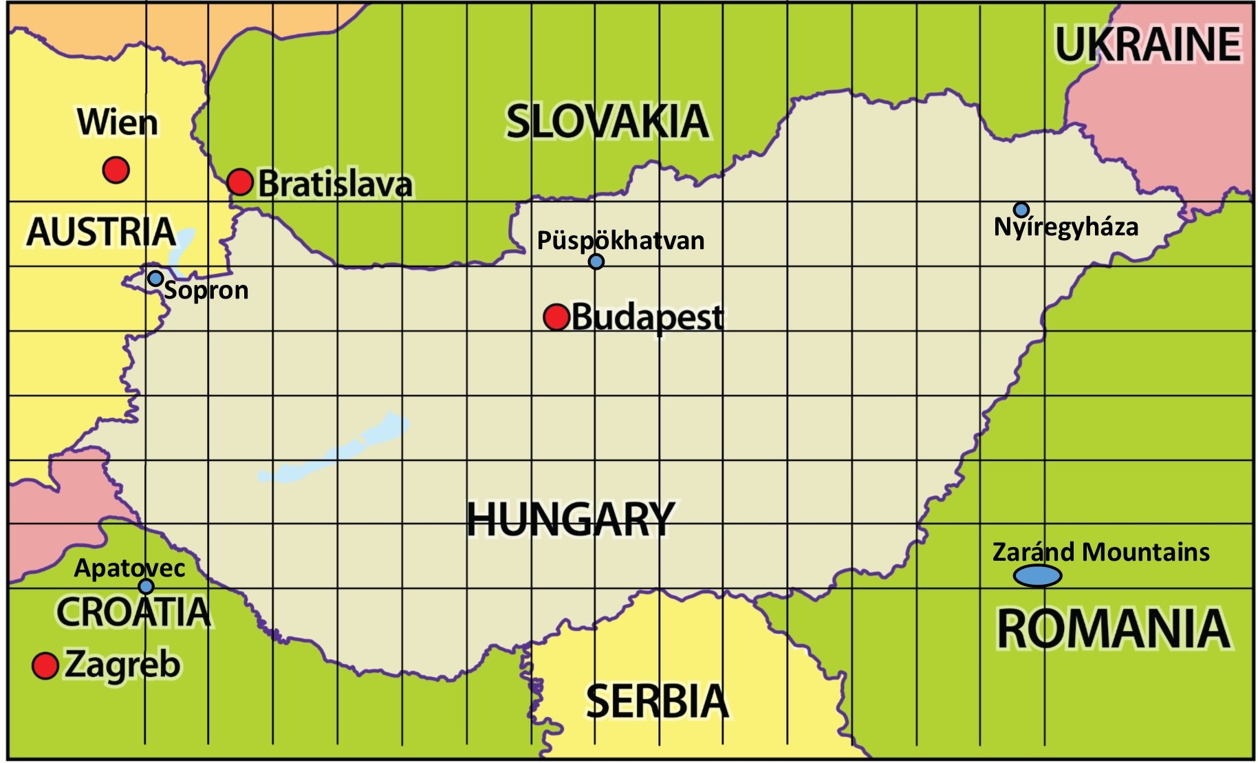
Figure 2: The map of the Carpathian Basin with the used grid points.

As we intend to use models, suitable for stationary data, first the stationarity had to be ensured. We have first subtracted the smoothed daily averages from the observations. The smoothing was made by loess regression, Figure 3a.) and Figure 3b.) depict the daily averages and standard deviations of the 63 years’ data and the smoothing regression line for grid point Budapest. It turned out that the second-order stationarity is still far from being true (in winter the variances were substantially larger than in summer), so we have divided the observations with the smoothed estimated standard deviation for the given day:

$$\tilde{x}_{t,n}=\frac{x_{t,n}-m_{t}}{s_{t}}$$

where $\tilde{x}_{t,n}$ is the standardized value for day $t$ in year $n$, based on the original observation $x_{t,n}$ for the same day and the smoothed average $m_{t}$ and smoothed standard deviation $s_{t}$. Figure 3c.) shows the original daily observations and the standardized data between January 1, 2010 and December 31, 2012 for grid point Budapest.

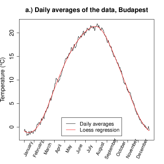
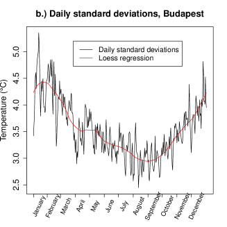
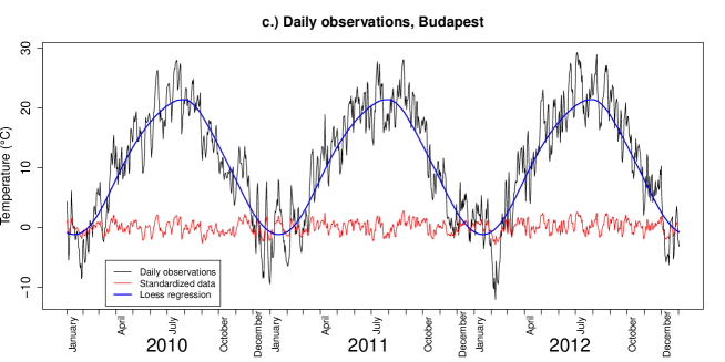
Figure 3: a.) The daily averages (annual cycle) and the smoothing loess regression; the daily standard deviations (annual cycle) and the smoothing loess regression; c.) the original and the standardized data for grid point Budapest.

In order to reduce the effect of the outliers of our results, we have finally computed the ten-days averages of the $\tilde{x}$ values. There is a slight but significant upward linear trend in the data, but we did not remove it, as one of our main aims was to detect the changes in the dependencies of the investigated sites – and these should be based on the original (standardised) deviations, as constructed above.

In the next step, we examined the fixed grid point Budapest paired with other grid points of the database. Using the Akaike information criterion, we chose the lags of the most appropriate among vector autoregressions to model our data pairs. Despite the adjusted $R^{2}$ values being rather low (around 10%), the Ljung-Box Q-test, the Breusch-Godfrey test and the test of Kojadinovic and Yan (2011) could not detect the presence of further serial dependence that has not been included in the VAR model. Table 1 contains these results.

Table 1: Results of tests checking for serial dependence between the estimated residuals (p-values) and the chosen lag of the VAR model by Akaike criterion.

Pairs of selected grid points	Optimal	Ljung-	Breusch-	Genest-Rémillard-
	lag	Box	Godfrey	Kojadinovic-Yan
Budapest & Sopron	3	0.271	0.324	0.259
Budapest & Apatovac	1	0.080	0.463	0.120
Budapest & Zaránd Mountains	9	0.174	0.017	0.149
Budapest & Nyíregyháza	4	0.174	0.474	0.258
Budapest & Püspökhatvan	4	0.155	0.539	0.276

Our main goal is to detect if there is a significant change in the dependence structure of the data. We separated the pairs of points into two parts – the first part corresponds to the first 31.5 years’ observations and the second part to the second 31.5 years’ observations. For five selected pairs of grid points, we wanted to test the null hypothesis if the copula of first half of the sample is equal to the copula of the second half of the sample.

Table 2 and Figure 4 depict the optimal block lengths obtained from solving equation (5). The second column of Table 2 and the red line of Figure 5 show the trace of the covariance matrices of the mean, calculated from the fitted VAR(1) models, multiplicated by 1186 – the half of the original sample size. We can see on the left figure that the trace of the covariance matrix of the mean is not monotone in the neighborhood of the optimum, so we have to be cautious. The trace function (black line in Figure 5) is always continuous, but not necessarily differentiable, resulting from the construction of our generalized block bootstrap method. Generally, we noticed, that as the block sizes tend to be smaller, the trace function is nearer to be monotonic. This phenomenon can be explained by the expansion of $\text{Cov}_{*}(\overline{X}_{b}^{*})$ in formula (6): if the block size is relatively small compared to the sample size, then the first and second terms are much more dominant over the third part – which contains the effect of the remainder block size. We got pretty small, 6.51 optimal block size for the pairs Budapest & Zaránd Mountains and 20.43 for Budapest & Sopron. In case of the five selected pairs, as many as 7 iterations were always enough to solve equation (5). We have to mention that there exist some pairs of grid points – especially at the southern part of the Carpathian Basin –, for which equation (5) is not solvable.

Table 2: Optimal block length for the first half of the samples for the five selected pairs of grid points.

Pairs of selected grid points	$n\cdot\text{tr}\left(\text{Cov}(\overline{X}_{\!V\!\!A\!R})\right)$	Optimal	Number of
		block size	iterations
Budapest & Sopron	1.87	20.43	4
Budapest & Apatovac	1.92	11.23	3
Budapest & Zaránd Mountains	2.00	16.51	3
Budapest & Nyíregyháza	1.84	19.34	3
Budapest & Püspökhatvan	1.92	32.35	7

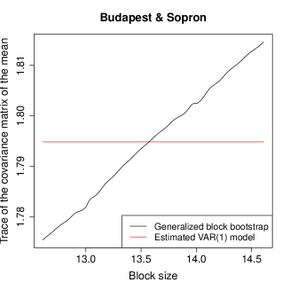
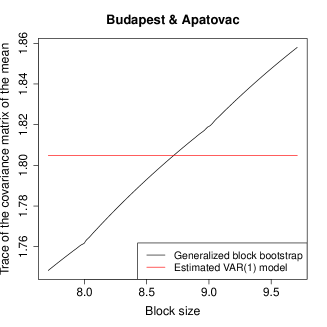
Figure 4: The trace of the covariance matrix of the mean for two selected grid points (first half of the sample).

The last step was conducting the copula homogeneity test described in Section 3. Using the optimal block size, we generated boostrap samples via the generalized block bootstrap method for the first half of the sample. With the empirical copulas of these boostrap samples and the empirical copula of the second part of the original sample, we can calculate the test statistic $S_{n,m}$. In our case $n=m=1186$. In order to get accurate $p$-values, we used 2000 repetitions. Table 3 contains the results of the homogeneity test. The dependence structure proved to be different in the first 31.5 years at the two pairs Budapest & Apatovac and Budapest & Zaránd Mountains. Figure 5 depicts the standarized observations and their copula of the pair Budapest & Apatovac. We can see that preudo-observations are apparently somewhat different, and the test also detected deviance between the two copulas.

Table 3: $p$-values of the copula homogeneity test, based on 2000 simulations.

Pairs of selected grid points	$p$-values
Budapest & Sopron	0.064
Budapest & Apatovac	0.028
Budapest & Zaránd Mountains	0.034
Budapest & Nyíregyháza	0.116
Budapest & Püspökhatvan	0.848

Figure 5: The pseudo-observations of Budapest & Apatovac for the first and the second half of the sample.

6 Conclusions

We can summarize our results as follows.

There are two major points to be mentioned. First, we proposed a simple generalisation of the block bootstrap methodology, which fits naturally to the existing algorithms, and which helps to overcome the problem of discreteness in the usual block size. Second, we have found some significant changes in the dependence structure between the standardised temperature values of pairs of stations within the Carpathian Basin. The direction of this change may be worth for investigating, as this may lead to a better understanding of the processes of our climate.

The proposed generalized block bootstrap method can easily be applied to any other problem, where the block size plays an important role, as all block length determining algorithms give a real number as estimated block size.

It is an interesting question, to which models the proposed block size determining method can be successfully applied. We have checked by simulation that the method is reasonably stable for the VAR models, presented in the paper. For nonlinear time series we might need more observations to fit, which is similarly reliable as the one, presented in our paper.

Acknowledgements
We acknowledge the E-OBS dataset from the EU-FP6 project ENSEMBLES (http://ensembles-eu.metoffice.com) and the data providers in the ECA&D project (http://www.ecad.eu).

References

- Brockwell and Davis (2013) P. J. Brockwell and R. A. Davis. Time series: theory and methods. Springer Science & Business Media, 2013.
- Chernick (2011) M. R Chernick. Bootstrap methods: A guide for practitioners and researchers, volume 619. John Wiley & Sons, 2011.
- Cong and Brady (2012) R.-G. Cong and M. Brady. The interdependence between rainfall and temperature: copula analyses. The Scientific World Journal, 2012, 2012.
- Efron (1979) B. Efron. Bootstrap methods: another look at the jackknife. The Annals of Statistics, 7(1), 1979.
- Farook and Kannan (2016) A. Jawahar Farook and K. Senthamarai Kannan. Climate change impact on rice yield in india–vector autoregression approach. Sri Lankan Journal of Applied Statistics, 16(3), 2016.
- Genest et al. (2006) C. Genest, J.-F. Quessy, and B. Rémillard. Goodness-of-fit procedures for copula models based on the probability integral transformation. Scandinavian Journal of Statistics, 33(2):337–366, 2006.
- Genest and Rémillard (2004) Christian Genest and Bruno Rémillard. Test of independence and randomness based on the empirical copula process. Test, 13(2):335–369, 2004.
- Hall et al. (1995) P. Hall, J. L. Horowitz, and B.-Y. Jing. On blocking rules for the bootstrap with dependent data. Biometrika, 82(3):561–574, 1995.
- Haylock et al. (2008) M. Haylock, N. Hofstra, A. M. G. Klein Tank, E. J. Klok, P. D. Jones, and M. New. A European daily high-resolution gridded data set of surface temperature and precipitation for 1950–2006. Journal of Geophysical Research: Atmospheres (1984–2012), 113(D20), 2008.
- Hill et al. (2014) D. Hill, K. Bell, D. McMillan, and D. Infield. A vector auto-regressive model for onshore and offshore wind synthesis incorporating meteorological model information. Advances in Science and Research, 11:35–39, 2014.
- Hoeffding (1940) W. Hoeffding. Massstabinvariante korrelationstheorie. Teubner, 1940.
- Hofstra et al. (2009) N. Hofstra, M. Haylock, M. New, and P. D. Jones. Testing e-obs european high-resolution gridded data set of daily precipitation and surface temperature. Journal of Geophysical Research: Atmospheres, 114(D21), 2009.
- Kojadinovic and Yan (2011) Ivan Kojadinovic and Jun Yan. Tests of serial independence for continuous multivariate time series based on a möbius decomposition of the independence empirical copula process. Annals of the Institute of Statistical Mathematics, 63(2):347–373, 2011.
- Lahiri (2003) S. N. Lahiri. Resampling methods for dependent data. Springer Science & Business Media, 2003.
- Nelsen (2007) R. B. Nelsen. An introduction to copulas. Springer Science & Business Media, 2007.
- Norrulashikin et al. (2015) S. M. Norrulashikin, F. Yusof, and I. L. Kane. An investigation towards the suitability of vector autoregressive approach on modeling meteorological data. Modern Applied Science, 9(11):p89, 2015.
- Patton et al. (2009) A. Patton, D. N. Politis, and H. White. Correction to "automatic block-length selection for the dependent bootstrap" by d. politis and h. white. Econometric Reviews, 28(4):372–375, 2009.
- Politis and Romano (1994) D. N. Politis and J. P. Romano. The stationary bootstrap. Journal of the American Statistical association, 89(428):1303–1313, 1994.
- Politis and White (2004) D. N. Politis and H. White. Automatic block-length selection for the dependent bootstrap. Econometric Reviews, 23(1):53–70, 2004.
- Rakonczai et al. (2014) P. Rakonczai, L. Varga, and A. Zempléni. Copula fitting to autocorrelated data with applications to wind speed modelling. Annales Universitatis Scientarium de Rolando Eotvos Nominatae, Sectio Computatorica, 43:3–20, 2014.
- Rémillard and Scaillet (2009) B. Rémillard and O. Scaillet. Testing for equality between two copulas. Journal of Multivariate Analysis, 100(3):377–386, 2009.
- Shumway and Stoffer (2011) R. H. Shumway and D. S. Stoffer. Time series analysis and its applications with R examples. Springer Science & Business Media, 2011.
- Sims (1980) C. A. Sims. Macroeconomics and reality. Econometrica: Journal of the Econometric Society, pages 1–48, 1980.