Testing High Dimensional Covariance Matrices, with Application to Detecting Schizophrenia Risk Genes

Supplemental Materials

Scientists routinely compare gene expression levels in cases versus controls in part to determine genes associated with a disease. Similarly, detecting case-control differences in co-expression among genes can be critical to understanding complex human diseases; however statistical methods have been limited by the high dimensional nature of this problem. In this paper, we construct a sparse-Leading-Eigenvalue-Driven (sLED) test for comparing two high-dimensional covariance matrices. By focusing on the spectrum of the differential matrix, sLED provides a novel perspective that accommodates what we assume to be common, namely sparse and weak signals in gene expression data, and it is closely related with Sparse Principal Component Analysis. We prove that sLED achieves full power asymptotically under mild assumptions, and simulation studies verify that it outperforms other existing procedures under many biologically plausible scenarios. Applying sLED to the largest gene-expression dataset obtained from post-mortem brain tissue from Schizophrenia patients and controls, we provide a novel list of genes implicated in Schizophrenia and reveal intriguing patterns in gene co-expression change for Schizophrenia subjects. We also illustrate that sLED can be generalized to compare other gene-gene “relationship” matrices that are of practical interest, such as the weighted adjacency matrices.

, ,  and

Carnegie Mellon University^t1thankst1 and University of Pittsburgh^t2thankst2

1 Introduction

High throughput technologies provide the capacity for measuring potentially interesting genetic features on the scale of tens of thousands. With the goal of understanding various complex human diseases, a widely used technique is gene differential expression analysis, which focuses on the marginal effect of each variant. Converging evidence has also revealed the importance of co-expression among genes, but analytical techniques are still underdeveloped. Improved methods in this domain will enhance our understanding of how complex disease affects the patterns of gene expression, shedding light on both the development of disease and its pathological consequences.

Schizophrenia (SCZ), a severe mental disorder with 0.7% lifetime risk (McGrath et al., 2008), is one of the complex human traits that has been known for decades to be highly heritable but whose genetic etiology and pathological consequences remain unclear. What has been repeatedly confirmed is that a large proportion of SCZ liability traces to polygenetic variation involving many hundreds of genes together, with each variant exerting a small impact (Purcell et al., 2014; International Schizophrenia Consortium et al., 2009). Despite the large expected number, only a small fraction of risk loci have been conclusively identified (Schizophrenia Working Group of the Psychiatric Genomics Consortium, 2014). This failure is mainly due to the limited signal strength of individual variants and under-powered mean-based association studies. Still, several biological processes, including synaptic mechanisms and glutamatergic neurotransmission, have been reported to be implicated in the risk for SCZ (Fromer et al., 2016). The observation that each genetic variant contributes only moderately to risk, and that each affected individual carries many risk variants, suggests that SCZ develops as a consequence of subtle alterations of both gene expression and co-expression, which requires development of statistical methods to describe the subtle, wide-spread co-expression differences.

Pioneering efforts have started in this direction. Very recently, the CommonMind Consortium (CMC) completed a large-scale RNA sequencing on dorsolateral prefrontal cortex from 279 control and 258 SCZ subjects, forming the largest brain gene expression data set on SCZ (Fromer et al., 2016). Analyses of these data by the CommonMind Consortium suggest that many genes show altered expression between case and control subjects, although the mean differences are small. By combining gene expression and co-expression patterns with results from genetic association studies, it appears that genetic association signals tend to cluster in certain sets of tightly co-expressed genes, so called co-expression modules (Zhang and Horvath, 2005). Still, the study of how gene co-expression patterns change from controls to SCZ subjects remains incomplete. Here, we address this problem using a hypothesis test that compares the gene-gene covariance matrices between control and SCZ samples, with integrated variable selection.

The problem of two-sample test for covariance matrices has been thoroughly studied in traditional multivariate analysis (Anderson et al., 1958), but becomes nontrivial once we enter the high-dimensional regime. Most of the previous high-dimensional covariance testing methods are motivated by either the $L_{2}$-type distance between matrices where all entries are considered (Schott, 2007; Li and Chen, 2012), or the $L_{\infty}$-type distance where only the largest deviation is utilized (Cai, Liu and Xia, 2013; Chang et al., 2016). These two strategies are designed for two extreme situations, respectively: when almost all genes exhibit some difference in co-expression patterns, or when there is one “leading” pair of genes whose co-expression pattern has an extraordinary deviation in two populations. However, the mechanism of SCZ is most likely to lie somewhere in between, where the difference may occur among hundreds of genes (compared to a total of $\approx\,$20,000 human genes), yet each deviation remains small. Some other existing approaches include using the trace of the covariance matrices (Srivastava and Yanagihara, 2010), using random matrix projections (Wu and Li, 2015), and using energy statistics to measure the distance between two populations (Székely and Rizzo, 2013). But none of these methods are designed for the scenario in which the signals are both sparse and weak.

In this paper, we propose a sparse-Leading-Eigenvalue-Driven (sLED) test. It provides a novel perspective for matrix comparisons by evaluating the spectrum of the differential matrix, defined as the difference between two covariance matrices. This provides greater power and insight for many biologically plausible models, including the situation where only a small cluster of genes has abnormalities in SCZ subjects, so that the differential matrix is supported on a small sub-block. The test statistic of sLED links naturally to the fruitful results in Sparse Principle Component Analysis (SPCA), which is widely used for unsupervised dimension reduction in the high-dimensional regime. Both theoretical and simulation results verify that sLED has superior power under sparse and weak signals. In addition, sLED can be generalized to comparisons between other gene-gene “relationship” matrices, including the weighted adjacency matrices that are commonly used in gene clustering studies (Zhang and Horvath, 2005). Applying sLED to the CMC data sheds light on novel SCZ risk genes, and reveals intriguing patterns that are previously missed by the mean-based differential expression analysis.

For the rest of this paper, we motivate and propose sLED for testing two-sample covariance matrices in Section 2. We provide two algorithms to compute the test statistic, and establish theoretical guarantees on the asymptotic consistency. In Section 3, we conduct simulation studies and show that sLED has superior power to other existing two-sample covariance tests under many scenarios. In Section 4, we apply sLED to the CMC data. We detect a list of genes implicated in SCZ and reveal interesting patterns of gene co-expression changes. We also illustrate that sLED can be generalized to comparing weighted adjacency matrices. Section 5 concludes the paper and discusses the potential of applying sLED to other datasets. All proofs are included in the Supplement. An implementation of sLED is provided at https://github.com/lingxuez/sLED.

2 Methods

2.1 Background

Suppose $X_{1},\cdots,X_{n}\stackrel{{\scriptstyle i.i.d.}}{{\sim}}({\mathbf{0}}_{p},\Sigma_{1})$ and $Y_{1},\cdots,Y_{m}\stackrel{{\scriptstyle i.i.d.}}{{\sim}}({\mathbf{0}}_{p},\Sigma_{2})$ are independent $p$-dimensional random variables coming from two populations with potentially different covariance structures. Without loss of generality, both expectations are assumed to be zero, and let $D=\Sigma_{2}-\Sigma_{1}$ be the differential matrix. The goal is to test

$$H_{0}:\,D=0\ \textrm{versus }\ H_{1}:\,D\neq 0\,.$$ (2.1)

This two-sample covariance testing problem has been well studied in the traditional “large $n$, small $p$” setting, where the likelihood ratio test (LRT) is commonly used. However, testing covariance matrices under the high-dimensional regime is a nontrivial problem. In particular, LRT is no longer well defined when $p>\min\{n,m\}$. Even if $p\leq\min\{n,m\}$, LRT has been shown to perform poorly when $p/\min\{n,m\}\to c\in(0,1)$ (Bai et al., 2009).

Researchers have approached this problem in different ways. Here, we give detailed review on two of the main strategies to motivate our test. The first one starts from rewriting eq. 2.1 as

$$H_{0}:\,||D||_{F}^{2}=0\ \textrm{versus }\ H_{1}:\,||D||_{F}^{2}\neq 0\,,$$ (2.2)

where $||D||_{F}$ is the Frobenius norm of $D$. This strategy includes a test statistic based on an estimator of $||D||_{F}^{2}$ under normality assumptions (Schott, 2007), as well as a test under more general settings using a linear combination of three U-statistics, which is also motivated by $||D||_{F}^{2}$ (Li and Chen, 2012). These $L_{2}$-norm driven tests target a dense alternative, but usually suffer from loss of power when $D$ has only a small number of non-zero entries. On the other hand, Cai, Liu and Xia (2013) consider the sparse alternative, and rewrite eq. 2.1 as

$$H_{0}:\,||D||_{\infty}=0\ \textrm{versus }\ H_{1}:\,||D||_{\infty}\neq 0\,,$$ (2.3)

where $||D||_{\infty}=\max_{i,j}|D_{ij}|$. Then the test statistic is constructed using a normalized estimator of $||D||_{\infty}$. Later, Chang et al. (2016) propose a bootstrap procedure using the same test statistic but under weaker assumptions, and Cai and Zhang (2015) extend the idea to comparing two-sample correlation matrices. These $L_{\infty}$-norm based tests have been shown to enjoy superior power when the single-entry signal is strong, in the sense that $\max_{i,j}|D_{ij}|$ is of order $\sqrt{\log p/\min\{n,m\}}$ or larger.

In this paper, we focus on the unexplored but practically interesting regime where the signal is both sparse and weak, meaning that the difference may occur at only a small set of entries, while the magnitude tends to be small. We propose another perspective to construct the test statistic by looking at the singular value of $D$, which is especially suitable for this purpose. To illustrate the idea, consider a toy example where

$$D_{ij}=\begin{cases}\delta,&1\leq i,j\leq s\\ 0,&\textrm{otherwise}\end{cases}$$ (2.4)

for some $\delta>0$ and integer $s\ll p$. In other words, $\Sigma_{2}$ and $\Sigma_{1}$ are only different by $\delta$ in an $s\times s$ sub-block. In this case, the $L_{2}$-type tests are sub-optimal because they include errors from all entries; so are the $L_{\infty}$-type tests because they only utilize one single entry $\delta$. On the other hand, the largest singular value of $D$ is $s\delta$, which extracts stronger signals with much less noise and therefore has the potential to gain more power.

More formally, we rewrite the testing problem eq. 2.1 to be

$$\begin{split}&H_{0}:\,\sigma_{1}(D)=0\ \textrm{versus }\ H_{1}:\,\sigma_{1}(D)\neq 0\,,\end{split}$$ (2.5)

where $\sigma_{1}(\cdot)$ denotes the largest singular value. Compared to eq. 2.2 and eq. 2.3, eq. 2.5 provides a novel perspective to study the two-sample covariance testing problem based on the spectrum of the differential matrix $D$, and will be the starting point of constructing our test statistic.

Notation

For a vector $v\in\mathbb{R}^{p}$, let $||v||_{q}=\left(\sum_{i=1}^{p}|v_{i}|^{q}\right)^{1/q}$ be the $L_{q}$ norm for $q>0$, and $||v||_{0}$ be the number of non-zero elements. For a symmetric matrix $A\in\mathbb{R}^{p\times p}$, let $A_{ij}$ be the $(i,j)$-th element, $||A||_{q}$ be the $L_{q}$ norm of vectorized $A$, and ${\rm tr}(A)$ be the trace. In addition, we use $\lambda_{1}(A)\geq\cdots\geq\lambda_{p}(A)$ to denote the eigenvalues of $A$. For two symmetric matrices $A,B\in\mathbb{R}^{p\times p}$, we write $A\succeq B$ when $A-B$ is positive semidefinite. Finally, for two sequences of real numbers $\{x_{n}\}$ and $\{y_{n}\}$, we write $x_{n}=O(y_{n})$ if $|x_{n}/y_{n}|\leq C$ for all $n$ and some positive constant $C$, and $x_{n}=o(y_{n})$ if $\lim_{n}x_{n}/y_{n}=0$.

2.2 A two-sample covariance test: sLED

Starting from eq. 2.5, note that

$$\sigma_{1}(D)=\max\{\left|\lambda_{1}(D)\right|,\,\left|\lambda_{1}(-D)\right|\}\,.$$

Therefore, a naive test statistic would be $T^{\textrm{naive}}=\max\left\{\left|\lambda_{1}(\hat{D})\right|,\,\left|\lambda_{1}(-\hat{D})\right|\right\}$ for some estimator $\hat{D}$. A simple estimator is the difference between the sample covariance matrices:

$$\hat{D}=\hat{\Sigma}_{2}-\hat{\Sigma}_{1}\,,\\ \textrm{where }\hat{\Sigma}_{1}=\frac{1}{n}\sum_{k=1}^{n}X_{k}X_{k}^{T}\,,\ \hat{\Sigma}_{2}=\frac{1}{m}\sum_{l=1}^{m}Y_{l}Y_{l}^{T}\,.$$ (2.6)

However, in the high-dimensional setting, $\lambda_{1}(\hat{D})$ is not necessarily a consistent estimator of $\lambda_{1}(D)$, and without extra assumptions, there is almost no hope of reliable recovery of the eigenvectors (Johnstone and Lu, 2009). A popular remedy for this curse of dimensionality in many high-dimensional methods is to add sparsity assumptions, such as imposing an $L_{0}$ constraint on an optimization procedure. Note that for any symmetric matrix $A\in\mathbb{R}^{p\times p}$,

$$\lambda_{1}(A)=\max_{||v||_{2}=1}v^{T}Av=\max_{||v||_{2}=1}{\rm tr}\left(A(vv^{T})\right)\,.$$

Following the common strategy, we consider the constrained problem:

$$\lambda_{1}^{R}(A)=\max_{||v||_{2}=1,\,||v||_{0}\leq R}{\rm tr}\left(A(vv^{T})\right)\,,$$ (2.7)

where $R>0$ is some constant that controls the sparsity of the solution, and $\lambda_{1}^{R}(A)$ is usually referred to as the $R$-sparse leading eigenvalue of $A$. Then, naturally, we construct the following test statistic

$$T_{R}=\max\left\{\left|\lambda_{1}^{R}(\hat{D})\right|,\,\left|\lambda_{1}^{R}(-\hat{D})\right|\right\}\,,$$ (2.8)

and the sparse-Leading-Eigenvalue-Driven (sLED) test is obtained by thresholding $T_{R}$ at the proper level.

Problem eq. 2.7 is closely related with Sparse Principle Component Analysis (SPCA). The only difference is that in SPCA, the input matrix $A$ is usually the sample covariance matrix, but here, we use the differential matrix $\hat{D}$. Solving eq. 2.7 directly is computationally intractable, but we will show in Section 2.3 that approximate solutions can be obtained.

Finally, because it is difficult to obtain the limiting distribution of $T_{R}$, we use a permutation procedure. Specifically, for any $\alpha\in(0,1)$, the $\alpha-$level sLED test, denoted by $\Psi_{\alpha}$, is conducted as follows:

1. Given samples $Z=(X_{1},\cdots,X_{n},Y_{1},\cdots,Y_{m})$, calculate the test statistic $T_{R}$ as in eq. 2.8.

2. Sample uniformly from $Z$ without replacement to get $Z^{*}=(Z_{1}^{*},\cdots,Z_{N}^{*})$, where $N=n+m$.

3. Calculate the permutation differential matrix $\hat{D}^{*}$:

   $$\hat{D}^{*}=\hat{\Sigma}_{2}^{*}-\hat{\Sigma}_{1}^{*}\,,$$ (2.9)

   where $\hat{\Sigma}_{1}^{*}=\cfrac{1}{n}\sum_{k=1}^{n}Z_{k}^{*}(Z_{k}^{*})^{T}\,,\ \hat{\Sigma}_{2}^{*}=\cfrac{1}{m}\sum_{l=n+1}^{N}Z_{l}^{*}(Z_{l}^{*})^{T}$.

4. Compute the permutation test statistic

   $$T_{R}^{*}=\max\left\{\left|\lambda_{1}^{R}(\hat{D}^{*})\right|,\,\left|\lambda_{1}^{R}(-\hat{D}^{*})\right|\right\}\,.$$ (2.10)

5. Repeat items 2 to 4 for $B$ times to get $T_{R}^{*(1)},\cdots,T_{R}^{*(B)}$, then

   $$\hat{p}=\frac{1}{B}\sum_{b=1}^{B}I_{\{T_{R}^{*(b)}>T_{R}\}}\,,$$

   and sLED rejects $H_{0}$ if $\hat{p}<\alpha$, i.e., $\Psi_{\alpha}=I_{\{\hat{p}<\alpha\}}$.

Remark 1

We can also estimate the support of the $R$-sparse leading eigenvector of $D$, which provides a list of genes that are potentially involved in the disease. Without loss of generality, suppose $\lambda_{1}^{R}(\hat{D})>\lambda_{1}^{R}(-\hat{D})$, we define

$$\textrm{Leverage}\coloneqq\textrm{diag}(\hat{v}\hat{v}^{T})=(\hat{v}_{1}^{2},\cdots,\hat{v}_{p}^{2})^{T}\,,$$ (2.11)

where $\hat{v}$ is the $R$-sparse leading eigenvector of $\hat{D}$ in eq. 2.7. Then the elements with large leverage will be the candidate genes that have altered covariance structure between the two populations.

2.3 Sparse principle component analysis

Many studies on Sparse Principle Component Analysis (SPCA) have provided various algorithms to approximate eq. 2.7 when $A$ is the sample covariance matrix. Most techniques utilize an $L_{1}$ constraint to achieve both sparsity and computational efficiency. To name a few, Jolliffe, Trendafilov and Uddin (2003) form the SCoTLASS problem by directly replacing the $L_{0}$ constraint by $L_{1}$ constraint; Zou, Hastie and Tibshirani (2006) analyze the problem from a penalized regression perspective; Witten, Tibshirani and Hastie (2009) and Shen and Huang (2008) use the framework of low rank matrix completion and approximation; d’Aspremont et al. (2007) and Vu et al. (2013) consider the convex relaxation of eq. 2.7. Recent development of atomic norms also provides an alternative approach to deal with the $L_{0}$ constrained problems (for example, see Oymak et al. (2015)). For the purpose of this paper, we give details of only the following two SPCA algorithms that can be directly generalized to approximate eq. 2.7 with input matrix $\hat{D}$, the differential matrix.

Fantope projection and selection (FPS)

For a symmetric matrix $A\in\mathbb{R}^{p\times p}$, FPS (Vu et al., 2013) considers a convex optimization problem:

$$\lambda_{fps}^{R}(A)=\max_{H\in\mathcal{F}^{1},\,||H||_{1}\leq R}{\rm tr}(AH)\,,$$ (2.12)

where $\mathcal{F}^{1}=\{H\in\mathbb{R}^{p\times p}:{\rm symmetric,}\ 0\preceq H\preceq I,\ {\rm tr}(H)=1\}$ is the 1-dimensional Fantope, which is the convex hull of all 1-dimensional projection matrices $\{vv^{T}:||v||_{2}=1\}$. In addition, by the Cauchy-Schwarz inequality, if $||v||_{2}=1$, then $||vv^{T}||_{1}\leq||v||_{0}$. Therefore, eq. 2.12 is a convex relaxation of eq. 2.7. Moreover, when the input matrix is $\hat{D}$, the problem is still convex, and the ADMM algorithm proposed in Vu et al. (2013) can be directly applied. This algorithm has guaranteed convergence, but requires iteratively performing SVD on a $p\times p$ matrix. Moreover, the calculation needs to be repeated $B$ times in the permutation procedure, and becomes computationally demanding when $p$ is on the order of a few thousands. Therefore, we present an alternative heuristic algorithm below, which is much more efficient and typically works well in practice.

Penalized matrix decomposition (PMD)

For a general matrix $A\in\mathbb{R}^{p\times p}$, PMD (Witten, Tibshirani and Hastie, 2009) solves a rank-one matrix completion problem:

$$\begin{gathered}\lambda_{pmd}^{R}(A)=\max_{u,v}\textrm{tr}\left(A\left(uv^{T}\right)\right)\,,\\ \textrm{subject to }||u||_{2}\leq 1,\,||v||_{2}\leq 1,\,||u||_{1}\leq\sqrt{R},\,||v||_{1}\leq\sqrt{R}\,.\end{gathered}$$ (2.13)

The solution for each one of $u$ and $v$ has a simple closed form after fixing the other one. This leads to a straightforward iterative algorithm, which has been implemented in the R package PMA. Moreover, if the solutions satisfy $\hat{u}=\hat{v}$, then they are also the solutions to the following non-convex Constrained-PMD problem:

$$\lambda_{c-pmd}^{R}(A)=\max_{||v||_{2}\leq 1,\,||v||_{1}\leq\sqrt{R}}\textrm{tr}\left(A\left(vv^{T}\right)\right)\,.$$ (2.14)

Note that the solutions of eq. 2.14 always have $||v||_{2}=1$, which implies $||v||_{1}^{2}=||vv^{T}||_{1}\leq||v||_{0}$, so eq. 2.14 is also an approximation to eq. 2.7. Now observe that when $A\succeq 0$, as in the usual SPCA setting, the solutions of eq. 2.13 automatically have $\hat{u}=\hat{v}$ by the Cauchy-Schwarz inequality. However, this is no longer true when $A$ is not positive semidefinite, as when we deal with the differential matrix $\hat{D}$. To overcome this issue, we choose some constant $d>0$ that is large enough such that $A+dI\succeq 0$. Then the solutions of $\lambda_{pmd}^{R}(A+dI)$ will satisfy $\hat{u}=\hat{v}$, and it is easy to obtain $\lambda_{c-pmd}^{R}(A)$ by

$$\lambda_{c-pmd}^{R}(A)=\lambda_{pmd}^{R}(A+dI)-d\,.$$ (2.15)

2.4 Consistency

Finally, we show that sLED is asymptotically consistent. The validity of its size is guaranteed by the permutation procedure. Here, we prove that sLED also achieves full power asymptotically, under the following assumptions:

1. (Balanced sample sizes) $\underline{c}n\leq m\leq\bar{c}n$ for some constants $0<\underline{c}\leq 1\leq\bar{c}<\infty$.

2. (Sub-gaussian tail) Let $(Z_{1},\cdots,Z_{N})=(X_{1},\cdots,X_{n},Y_{1},\cdots,Y_{m})$, then every $Z_{k}$ is sub-gaussian with parameter $\nu^{2}$, that is,

   $$\mathbb{E}\left[e^{t(Z_{k}^{T}u)}\right]\leq e^{\frac{t^{2}\nu^{2}}{2}},\quad\forall t>0,\,\forall u\in\mathbb{R}^{p}\textrm{ such that }||u||_{2}=1\,.$$

3. (Dimensionality) $(\log p)^{3}=O(n)$.

4. (Signal strength) Under $H_{1}$, for some constant $C$ to be specified later,

   $$\max\left\{\lambda_{1}^{R}(D),\ \lambda_{1}^{R}(-D)\right\}\geq CR\sqrt{\frac{\log p}{n}}\,.$$

Theorem 1 (Power of sLED).

Let $T_{R}$ be the test statistic as defined in eq. 2.8, and $T_{R}^{*}$ be the permutation test statistic as defined in eq. 2.10, where $\lambda_{1}^{R}(\cdot)$ is approximated by the $L_{1}$ constrained algorithms eq. 2.12 or eq. 2.14. Then under assumptions (A1)-(A3), for $\forall\delta>0$, there exists a constant $C$ depending on $(\underline{c},\bar{c},\nu^{2},\delta)$, such that if assumption (A4) holds, and $n,p$ are sufficiently large,

$$\mathbb{P}_{H_{1}}\left(T_{R}(\hat{D}^{*})>T_{R}(\hat{D})\right)\leq\delta\,.$$

As a consequence, for any pre-specified level $\alpha\in(0,1)$, pick $\delta=\alpha/2$, then

$$\mathbb{P}_{H_{1}}\left(\Psi_{\alpha}=1\right)\to 1\ \textrm{ as }B\to+\infty\,.$$

The proof of Theorem 1 contains two steps. First, Theorem 2 provides an upper bound of the entries in $\hat{D}^{*}$. Then Theorem 3 ensures that the permutation test statistic $T_{R}^{*}$ is controlled by $||\hat{D}^{*}||_{\infty}$, and the test statistic $T_{R}$ is lower-bounded in terms of the signal strength. We state Theorem 2 and Theorem 3 below, and the proof details are included in the Supplement.

Theorem 2 (Permutation differential matrix).

Under assumptions (A1)-(A3), let $\hat{D}^{*}$ be the permutation differential matrix as defined in eq. 2.9, then $\forall\delta>0$, there exist constants $C$, $C_{1}$ depending on $(\nu^{2},\underline{c},\bar{c})$, such that if $n,p$ are sufficiently large,

$$\mathbb{P}\left(||\hat{D}^{*}||_{\infty}>C\sqrt{\frac{\log(C_{1}p^{2}/\delta)}{n}}\right)\leq\delta\,.$$

Theorem 3 (Test statistic).

For any symmetric matrix $\hat{D}$, let $\tilde{\lambda}_{1}^{R}(\hat{D})$ be a solution of the $L_{1}$ constrained algorithms eq. 2.12 or eq. 2.14, then the following statements hold:

1. If $||\hat{D}||_{\infty}\leq\delta$, then $\tilde{\lambda}_{1}^{R}(\hat{D})\leq R\delta$.

2. If there is a matrix $D$ such that $||\hat{D}-D||_{\infty}\leq\delta$, then

   $$\tilde{\lambda}_{1}^{R}(\hat{D})\geq\lambda_{1}^{R}(D)-R\delta\,.$$

Remark 2

Assumption (A4) does not require the leading eigenvector of $D$ (or $-D$) to be sparse, only that the sparse signal be strong enough, which is a very mild requirement. In addition, the required sparse signal level, $O\left(R\sqrt{\log p/n}\right)$, has been shown to be the optimal detection rate for any polynomial-time algorithm under a similar setting (Berthet and Rigollet, 2013).

In fact, Berthet and Rigollet (2013) also show that without the computational constraint, the optimal signal strength is of order $O\left(\sqrt{R\log p/n}\right)$. Here, we show that this rate can also be achieved by sLED if we use the exact solutions of the $L_{0}$ constrained problem eq. 2.7. For this purpose, we introduce two slightly different assumptions as follows:

• (Dimensionality) $R=o(p),\ R^{5}(\log p)^{3}=O(n)$.

• (Signal strength) Under $H_{1}$, for some constant $C$ to be specified later,

  $$\max\left\{\lambda_{1}^{R}(D),\ \lambda_{1}^{R}(-D)\right\}\geq C\sqrt{\frac{R\log p}{n}}\,.$$

Now we state the results regarding the $L_{0}$ constrained solutions, and the proofs are included in the Supplement.

Theorem 4 (Power of sLED without computational constraint).

Let $T_{R}$ be the test statistic as defined in eq. 2.8 with $\lambda_{1}^{R}(\cdot)$ being a global optimum of eq. 2.7. Then under assumptions (A1)-(A2) and (A3’), for any pre-specified level $\alpha\in(0,1)$, there exists a constant $C$ depending on $(\underline{c},\bar{c},\nu^{2},\alpha)$, such that if assumption (A4’) holds, and $n,p$ are sufficiently large,

$$\mathbb{P}_{H_{1}}\left(\Psi_{\alpha}=1\right)\to 1\ \textrm{ as }B\to+\infty\,.$$

Remark 3

Recall the toy example in eq. 2.4. If we let $R=s$, then the $R$-sparse leading eigenvalue of $D$ is $\lambda_{1}^{R}(D)=s\delta$, and sLED remains powerful for $\delta$ as small as $O\left(\sqrt{\log p/(ns)}\right)$. On the other hand, the maximal entry method (Cai, Liu and Xia, 2013) cannot succeed under this setting since it requires $\delta$ to be of order $O\left(\sqrt{\log p/n}\right)$ or higher.

Remark 4

One might notice that under the toy example in eq. 2.4, assumption (A4) in Theorem 1 for the $L_{1}$ constrained sLED implies $\delta\geq C\sqrt{\log p/n}$, which is also the required rate for the maximal entry method (Cai, Liu and Xia, 2013). However, we shall view the theoretical results in Theorem 1 as a “sanity check”, in the sense that sLED is at least as good as the maximal entry test. We know that the maximal entry test will fail when $\delta$ is much smaller than $\sqrt{\log p/n}$, while our theory says that sLED will succeed whenever the maximal entry method succeeds. This is a worst case guarantee for sLED. In practice, sLED will often output $L_{0}$-sparse solutions, and Theorem 4 demonstrates the potential of sLED when the solution also happens to be $L_{0}$-sparse.

2.5 Choosing sparsity parameter $R$

The tuning parameter $R$ in eq. 2.12 and eq. 2.14 plays an important role in sLED test. If $R$ is too large, the method uses little regularization and assumption (A4) is unlikely to hold. If $R$ is too small, then the constraint is too strong to cover the signal in the differential matrix. The practical success of sLED requires an appropriate choice of $R$. We know that $R$ provides a natural, but possibly loose, lower bound on the support size of the estimated sparse eigenvector. In general, one can use cross-validation to choose $R$, so that the estimated leading sparse singular vector maximizes its inner product with a differential matrix computed from a testing subsample.

In applications, one can often choose $R$ with the aid of subject background knowledge and the context of subsequent analysis. For example, in the detection of Schizophrenia risk genes, we typically expect to report a certain proportion in a collection of genes for further investigation. Thus one can choose from a set of candidate values of $R$ to match the desired number of discoveries. In this paper, following Witten, Tibshirani and Hastie (2009), we use algorithm eq. 2.14 and choose the sparsity parameter $R$ to be

$$\sqrt{R}=c\sqrt{p}\,,~{}\textrm{for some}~{}c\in(0,1)\,,$$ (2.16)

then $c^{2}$ provides a loose lower bound on the proportion of selected genes. We will illustrate in simulation studies (Section 3) and the CMC data application (Section 4) that sLED is stable with a reasonable range of $c$.

3 Simulations

In this section, we conduct simulation studies to compare the power of sLED with other existing methods: Schott (2007) use an estimator of the Frobenius norm $||D||_{F}^{2}$ (Sfrob); Li and Chen (2012) use a linear combination of three U-statistics which is also motivated by $||D||_{F}^{2}$ (Ustat); Cai, Liu and Xia (2013) use the maximal absolute entry of $D$ (Max); Chang et al. (2016) use a multiplier bootstrap on the same test statistic (MBoot), and Wu and Li (2015) use random matrix projections (RProj). To obtain a fair comparison of empirical power, we use permutation to compute the $p$-values for all methods, except for MBoot, which already uses a bootstrap procedure. Because the empirical size is properly controlled by permutation, we focus on comparing the empirical power in the rest of this section. The simulation results in this section can be reproduced using the code provided at https://github.com/lingxuez/sLED.

We consider four different covariance structures of $\Sigma_{1}$ and $\Sigma_{2}=\Sigma_{1}+D$ under the alternative hypothesis. Under each scenario $i=1,\cdots,4$, we first generate a base matrix $\Sigma^{*(i)}$, and we enforce positive definiteness using $\Sigma_{1}=\Sigma^{*(i)}+\delta I_{p}$ and $\Sigma_{2}=\Sigma^{*(i)}+D+\delta I_{p}$, where $\delta=\left|\min\{\lambda_{\min}(\Sigma^{*(i)}),\lambda_{\min}(\Sigma^{*(i)}+D)\}\right|+0.05$. Now we specify the structures of $\{\Sigma^{*(i)}\}_{i=1,...,4}$. Under each scenario, we let $\Lambda\in\mathbb{R}^{p\times p}$ to be a diagonal matrix with diagonal elements being sampled from $\textrm{Unif}(0.5,2.5)$ independently. We denote $\lfloor x\rfloor$ to be the largest integer that is smaller than or equal to $x$.

1. Noisy diagonal. Let $\Delta^{(1)}_{ii}=1$, $\Delta^{(1)}_{ij}\sim\textrm{Bernoulli}(0.05)$ when $i<j$, and $\Delta^{(1)}_{ij}=\Delta^{(1)}_{ji}$ when $i>j$ for symmetry, and we define $\Sigma^{*(1)}=\Lambda^{1/2}\Delta^{(1)}\Lambda^{1/2}$. This model is also considered in Cai, Liu and Xia (2013).

2. Block diagonal. Let $K=\lfloor p/10\rfloor$ be the number of blocks, $\Delta^{(2)}_{ii}=1$, $\Delta^{(2)}_{ij}=0.55$ when $10(k-1)+1\leq i\neq j\leq 10k$ for $k=1,\cdots,K$, and zero otherwise. We define $\Sigma^{*(2)}=\Lambda^{1/2}\Delta^{(2)}\Lambda^{1/2}$. This model is also considered in Cai, Liu and Xia (2013) and Chang et al. (2016).

3. Exponential decay. Let $\Delta^{(3)}_{ij}=0.5^{|i-j|}$, and $\Sigma^{*(3)}=\Lambda^{1/2}\Delta^{(3)}\Lambda^{1/2}$. This model is also considered in Cai, Liu and Xia (2013) and Chang et al. (2016).

4. WGCNA. Here we construct $\Sigma^{*(4)}$ based on the CMC data (Fromer et al., 2016) using the simulation tool provided by WGCNA (Zhang and Horvath, 2005). Specifically, we first compute the eigengene (i.e., the first principal component) of the M2c module for the 279 control samples. The M2c module will be the focus of Section 4, and more detailed discussion is provided there. We use the simulateDatExpr command in the WGCNA R package to simulate new expressions for $p$ genes of the 279 samples. We set modProportions=(.8,.2), such that 80% of the $p$ genes are simulated to be correlated with the M2c eigengene, and the other $20\%$ genes are randomly generated. Default values are used for all other parameters. Finally, $\Sigma^{*(4)}$ is set to be the sample covariance matrix.

We consider the following two types of differential matrix $D$:

1. Sparse block difference. Suppose $D$ is supported on an $s\times s$ sub-block with $s=\lfloor 0.1p\rfloor$, and the non-zero entries are generated from $\textrm{Unif}(d/2,2d)$ independently. The signal level $d$ is chosen to be $d=\frac{1}{2}\sqrt{\left(\max_{1\leq j\leq p}\Sigma_{jj}^{*}\right)\log(p)}$ where $\Sigma^{*}$ is the base matrix defined above.

2. Soft-sparse spiked difference. Let $D$ be a rank-one matrix with $D=dvv^{T}$, where $v$ is a soft-sparse unit vector with $||v||_{2}=1$ and $||v||_{0}=\lfloor 0.2p\rfloor$. The support of $v$ is uniformly sampled from $\{1,\cdots,p\}$ without replacement. Among the non-zero elements, $\lfloor 0.1p\rfloor$ are sampled from $N(1,0.01)$, and the remaining $\lfloor 0.2p\rfloor-\lfloor 0.1p\rfloor$ are sampled from $N(0.1,0.01)$. Finally, $v$ is normalized to have unit $L_{2}$ norm. The signal level $d$ is set to be $d=4\sqrt{\left(\max_{1\leq j\leq p}\Sigma_{jj}^{*}\right)\log(p)}$, where $\Sigma^{*}$ is the base matrix defined above. The differential matrix $D$ under this scenario is moderately sparse, with $\lfloor 0.1p\rfloor$ features exerting larger signals.

Finally, the samples are generated by $X_{i}=\Sigma_{1}^{1/2}Z_{i}$ for $i=1,\cdots,n$, and $Y_{l}=\Sigma_{2}^{1/2}Z_{n+l}$ for $l=1,\cdots,m$, where $\{Z_{i}\}_{i=1,n+m}$ are independent $p$-dimensional random variables with $i.i.d.$ coordinates $Z_{ij}$, $j=1,\cdots,p$. We consider the following four distributions for $Z_{ij}$:

1. Standard Normal $N(0,1)$.

2. Centralized Gamma distribution with $\alpha=4,\beta=0.5$ (i.e., the theoretical expectation $\alpha\beta=2$ is subtracted from $\Gamma(4,0.5)$ samples). This distribution is also considered in Li and Chen (2012) and Cai, Liu and Xia (2013).

3. $t$-distribution with degrees of freedom 12. This distribution is also considered in Cai, Liu and Xia (2013) and Chang et al. (2016).

4. Centralized Negative Binomial distribution with mean $\mu=2$ and dispersion parameter $\phi=2$ (i.e., the theoretical expectation $\mu=2$ is subtracted from NB$(2,2)$ samples).

Note that when $Z_{ij}\sim N(0,1)$, $X$ and $Y$ are multinomial Gaussian random variables with covariance matrices $\Sigma_{1}$ and $\Sigma_{2}$. We also consider three non-Gaussian distributions to account for the heavy-tail scenario observed in many genetic data sets.

Here, the smoothing parameter for sLED is set to be $\sqrt{R}=0.3\sqrt{p}$, and 100 random projections are used for Rproj. For sLED, Max, Ustat, Sfrob, and Rproj, 100 permutations are used to obtain each $p$-value; for MBoot, 100 bootstrap repetitions are used. Table 1 summarizes the empirical power under different covariance structures and differential matrices when $Z_{ij}$’s are sampled from standard Normal and centralized Gamma distribution. We see that sLED is more powerful than many existing methods under most scenarios. The results using the other two distributions of $Z$ have similar patterns, and due to space limitation we include them in the Supplement.

Finally, we examine the sensitivity of sLED to the smoothing parameter. Recall that the smoothing parameter is set to be $\sqrt{R}=c\sqrt{p}$ as explained in Section 2.5. fig. 1 visualizes the empirical power of sLED using $c\in\{0.10,0.12,\cdots,0.30\}$ when $D$ has sparse block difference and $Z_{ij}$’s are sampled from $N(0,1)$. It is clear that sLED remains powerful for a wide range of $c$. Similar patterns are observed under other scenarios, and we include these results in the Supplement.

Table 1: Empirical power in 100 repetitions, where $n=m=100$, nominal level $\alpha=0.05$, and $Z_{ij}$’s are sampled from standard normal (top) and centralized Gamma $(4,0.5)$ (bottom). Under each scenario, the largest power is highlighted.

$\mathbf{D}$ $\mathbf{\Sigma_{1}}$ Noisy diagonal Block diagonal Exp. decay WGCNA $\mathbf{p}$ 100 200 500 100 200 500 100 200 500 100 200 500 Gaussian Block Max 0.38 0.14 0.11 0.94 0.54 0.25 0.98 0.86 0.31 0.92 0.64 0.16 MBoot 0.39 0.18 0.13 0.94 0.54 0.31 0.98 0.88 0.30 0.89 0.63 0.20 Ustat 0.71 0.66 0.74 0.98 0.96 0.95 1.00 1.00 0.99 0.76 0.78 0.85 Sfrob 0.72 0.64 0.73 0.97 0.95 0.95 1.00 1.00 0.99 0.72 0.79 0.86 RProj 0.09 0.13 0.09 0.13 0.16 0.14 0.24 0.16 0.09 0.20 0.17 0.06 sLED 1.00 0.99 1.00 1.00 0.99 1.00 1.00 1.00 1.00 0.98 0.96 0.95 Spiked Max 0.12 0.08 0.05 0.49 0.26 0.09 0.96 0.90 0.15 0.86 0.32 0.04 MBoot 0.12 0.08 0.05 0.51 0.29 0.11 0.98 0.90 0.17 0.79 0.31 0.07 Ustat 0.20 0.11 0.13 0.76 0.44 0.06 1.00 0.95 0.60 0.30 0.10 0.04 Sfrob 0.18 0.12 0.11 0.73 0.41 0.07 1.00 0.93 0.62 0.34 0.14 0.03 RProj 0.10 0.08 0.02 0.32 0.08 0.12 0.30 0.20 0.09 0.61 0.24 0.13 sLED 0.51 0.11 0.03 0.97 0.70 0.12 1.00 1.00 1.00 0.97 0.57 0.05 Centralized Gamma Block Max 0.42 0.20 0.14 0.89 0.71 0.28 0.96 0.82 0.42 0.77 0.67 0.27 MBoot 0.42 0.14 0.10 0.86 0.58 0.20 0.95 0.77 0.33 0.72 0.63 0.25 Ustat 0.57 0.59 0.70 0.92 0.94 0.97 0.99 0.98 0.98 0.53 0.82 0.86 Sfrob 0.58 0.55 0.71 0.92 0.92 0.98 0.99 0.99 0.98 0.50 0.76 0.81 RProj 0.11 0.10 0.09 0.24 0.17 0.16 0.41 0.15 0.14 0.21 0.07 0.14 sLED 0.96 0.98 0.99 0.99 1.00 1.00 1.00 1.00 1.00 0.94 0.88 0.94 Spiked Max 0.08 0.09 0.03 0.72 0.39 0.05 0.99 0.71 0.22 0.91 0.35 0.04 MBoot 0.10 0.07 0.02 0.74 0.36 0.09 0.99 0.71 0.16 0.88 0.35 0.04 Ustat 0.32 0.08 0.11 0.78 0.41 0.07 1.00 0.94 0.70 0.33 0.08 0.05 Sfrob 0.34 0.07 0.10 0.80 0.37 0.07 1.00 0.96 0.74 0.28 0.04 0.04 RProj 0.12 0.06 0.07 0.32 0.12 0.06 0.36 0.14 0.10 0.63 0.22 0.10 sLED 0.56 0.14 0.05 0.97 0.71 0.14 1.00 1.00 1.00 0.93 0.51 0.08

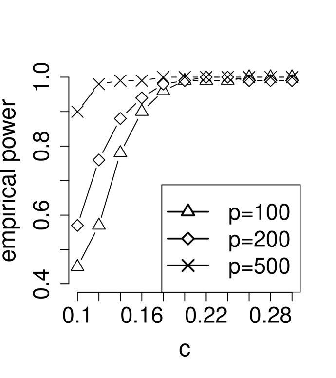
(a) Noisy diagonal

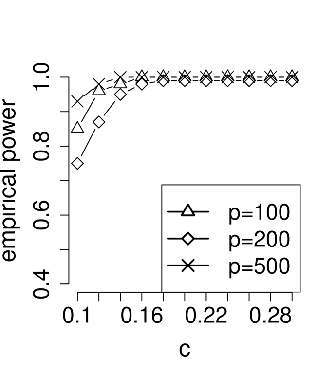
(b) Block diagonal

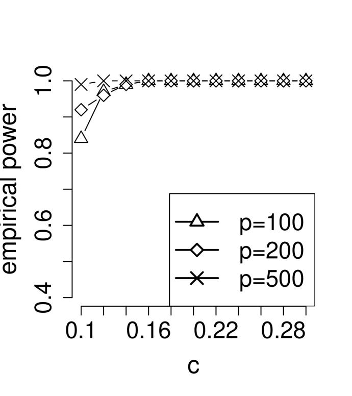
(c) Exp. decay

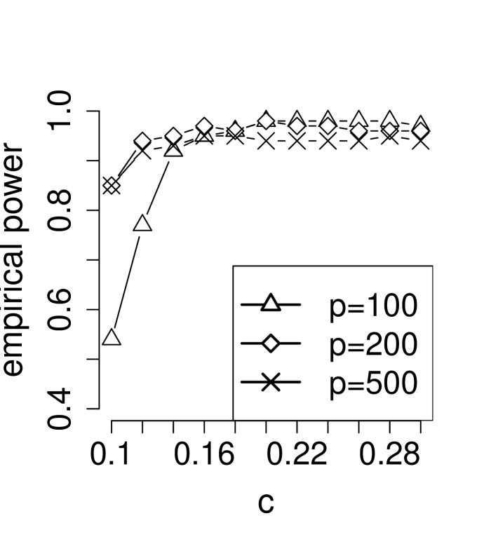
(d) WGCNA

Fig. 1: Empirical power of sLED in 100 repetitions using different smoothing parameters $\sqrt{R}=c\sqrt{p}$ for $c\in\{0.10,\cdots,0.30\}$, where $D$ has sparse block difference and $Z_{ij}$’s are sampled from $N(0,1)$.

4 Application to Schizophrenia data

In this section, we apply sLED to the CommonMind Consortium (CMC) data, containing RNA-sequencing on 16,423 genes from 258 Schizophrenia (SCZ) subjects and 279 control samples (Fromer et al., 2016). The RNA-seq data has been carefully processed, including log-transformation and correction of various covariates. The CMC group further cluster the genes into 35 genetic modules using the WGCNA tool (Zhang and Horvath, 2005), such that genes within each module tend to be closely connected and have related biological functionalities. Among these, the M2c module, containing 1,411 genes, is the only one that is enriched with genes exhibiting differential expression and with prior genetic associations with schizophrenia (SCZ). We direct readers to the original paper (Fromer et al., 2016) for more detailed description of the data processing and genetic module analysis. In the rest of this section, we apply sLED to investigate the co-expression differences between cases and controls in the M2c module, which is of the greatest scientific interest. We center and standardize the expression data, such that each gene has mean 0 and standard deviation 1 across samples. Therefore, the covariance test is applied to correlation matrices.

4.1 Testing co-expression differences

In this section, we use sLED to compare the correlation matrices among the 1,411 M2c-module genes between SCZ and control samples. The sparsity parameter in eq. 2.14 is chosen to be $\sqrt{R}=c\sqrt{p}$ as explained in Section 2.5. Here, because the number of risk genes that carry the genetic signals is expected to be roughly in the range of $1\%$–$10\%$, we choose $c=0.1$. Applying sLED with 1,000 permutation repetitions, we obtain a $p$-value of 0.014, indicating a significant difference between SCZ and control samples.

We then identify the key genes that drive this difference according to their leverage, as defined in eq. 2.11. Specifically, we order the leverage of all genes, such that $\hat{v}_{(1)}^{2}\geq\hat{v}_{(2)}^{2}\geq\cdots\geq\hat{v}_{(p)}^{2}$, where larger leverage usually indicates stronger signals. Note that by construction, $\sum_{i=1}^{p}\hat{v}_{(i)}^{2}=1$. Among the 1,411 genes, 113 genes have non-zero leverage, and we call them top genes. Moreover, we notice that the first 25 genes have already achieved a cumulative leverage of $0.999$, so we refer to them as primary genes. The remaining 88 top genes account for the rest $0.001$ leverage and are referred to as secondary genes (see fig. 2(a) for the visualization of this cut-off in a scree plot). We show in fig. 2(b) how these 113 top genes form a clear block structure in the differential matrix $\hat{D}=\hat{\Sigma}_{control}-\hat{\Sigma}_{SCZ}$. Notably, such a block structure cannot be revealed if ordered by the differentially expressed $p$-values (fig. 2(c)).

(a)

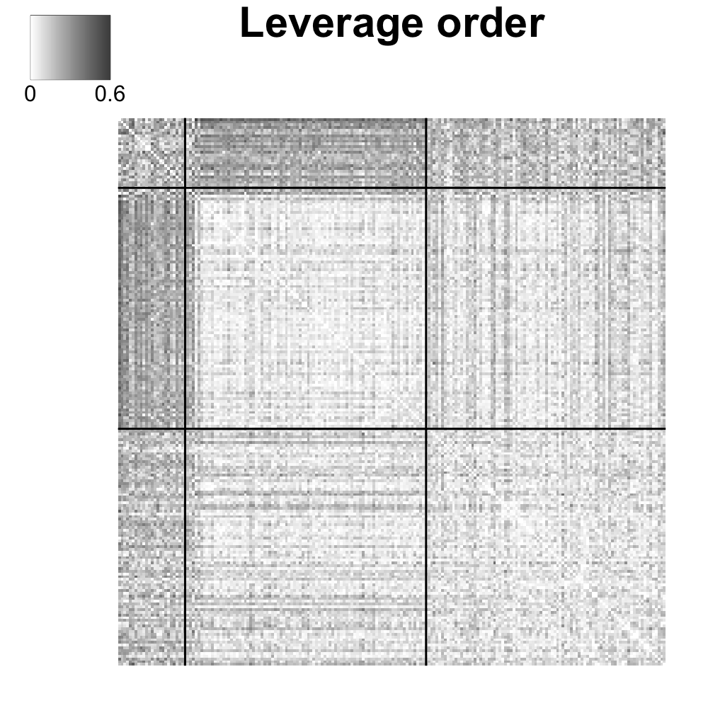
(b)

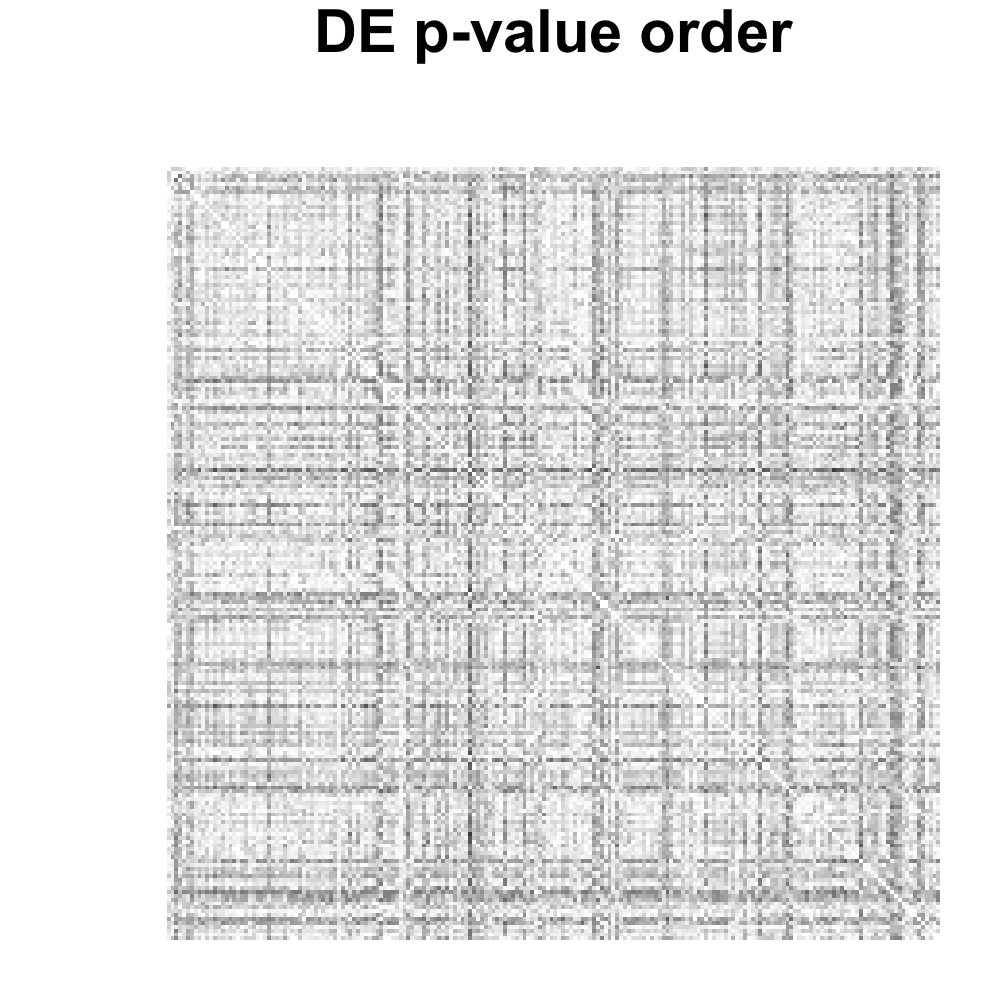
(c)

Fig. 2: Visualization of 200 genes in the M2c module, including 25 primary genes that account for a total leverage of 0.999, 88 secondary genes that account for the remaining 0.001 leverage, and 87 randomly selected other genes that have zero leverage. (a) Scree plot of cumulative leverage. (b) Heatmap of $|\hat{D}|$ where genes are ordered by leverage and a block structure is revealed. The two partitioning lines indicate the 25 primary genes and the 88 secondary genes. (c) Heatmap of $|\hat{D}|$ where genes are ordered by $p$-values in differential expression analysis. Now the block structure is diluted.

fig. 2(b) reveals a significant decrease of gene co-expression (interactions) in cortical samples from SCZ subjects between the 25 primary genes and the 88 secondary genes. This pattern is more clearly illustrated in fig. 3, where two gene networks are constructed for these 113 top genes in control samples and SCZ samples separately (see Table 2 for gene names).

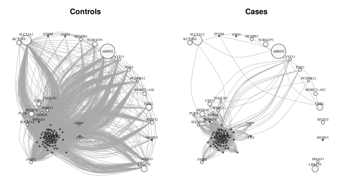
Fig. 3: Gene networks constructed from control and SCZ samples, using top genes in the M2c module that have non-zero leverage. We exclude 6 genes that do not have annotated gene names, and show the remaining 22 primary genes (colored in white) and 85 secondary genes (colored in grey). The adjacency matrix is constructed by thresholding the absolute Pearson correlation $|R_{ij}|$ at 0.5. Larger node sizes represent larger leverage.

Table 2: Annotated names of 22 primary genes and 85 secondary genes in the M2c module, listed in the descending order of leverage. The 6 underlined genes are also significant in the differential expression analysis

Gene names Primary genes ABHD2 SLC23A2 LRRC55 CRKL ZBTB24 TUBGCP3 KCTD10 USP13 MORC2-AS1 REXO2 HEXIM1 TOX3 FNIP2 WBP11 SYT11 SMAD3 SLC36A4 SNX30 PCDHB12 PURB TGOLN2 OSBP Secondary genes SH3RF1 IMPAD1 SYNM HECW2 ANO1 DNM3 STOX2 C1orf173 PPM1L DNAJC6 DLG2 LRRTM4 ANK3 EIF4G3 ANK2 ITSN1 SLIT2 LRRTM3 ATP8A2 CNTNAP2 CKAP5 GNPTAB USP32 USP9X ADAM23 SYNPO2 AKAP11 MAP1B KIAA1244 PPP1R12B SLC24A2 PTPRK SATB1 CAMTA1 MFSD6 KIAA1279 NTNG1 RYR2 RASAL2 PUM1 STAM ST8SIA3 ZKSCAN2 PBX1 ARHGAP24 RASA1 ANKRD17 MYCBP2 SLITRK1 BTRC MYH10 AKAP6 NRCAM MYO5A TRPC5 NRXN3 CACNA2D1 DNAJC16 GRIN2A KCNQ5 NETO1 FTO THRB NLGN1 HSPA12A BRAF OPRM1 KIAA1549L NOVA1 OPCML CEP170 DLGAP1 JPH1 LMO7 PCNX SYNJ1 RAPGEF2 NIPAL2 SYT1 UNC80 ATP8A1 SHROOM2 KCNJ6 SNAP91 WDR7

To shed light on the nature of the genes identified in the M2c module, we conduct a Gene Ontology (GO) enrichment analysis (Chen et al., 2013). The secondary gene list is most easily interpreted. It is highly enriched for genes directly involved in synaptic processes, both for GO Biological Process and Molecular Function. Two key molecular functions involve calcium channels/calcium ion transport and glutamate receptor activity. Under Biological Process, these themes are emphasized and synaptic organization emerges too. Synaptic function is a key feature that emerges from genetic findings for SCZ, including calcium channels/calcium ion transport and glutamate receptor activity (see Owen, Sawa and Mortensen (2016) for review).

For the primary genes, under GO Biological Process, “regulation of transforming growth factor beta2 (TGF-$\beta$2) production” is highly enriched. The top GO Molecular Function term is SMAD binding. The protein product of SMAD3 (one of the primary genes) modulates the impact of transcription factor TGF-$\beta$ regarding its regulation of expression of a wide set of genes. TGF-$\beta$ is important for many developmental processes, including the development and function of synapses (Diniz et al., 2012). Moreover, and notably, it has recently been shown that SMAD3 plays a crucial role in synaptogenesis and synaptic function via its modulation of how TGF-$\beta$ regulates gene expression (Yu et al., 2014). It is possible that disturbed TGF-$\beta$ signaling could explain co-expression patterns we observe in fig. 3, because this transcription factor will impact multiple genes. Another primary gene of interest is OSBP. Its protein product has recently been shown to regulate neural outgrowth and thus synaptic development (Gu et al., 2015). Thus perturbation of a set of genes could explain the pattern seen in fig. 3.

4.2 Robustness of the results

In this section, we illustrate that sLED remains powerful under perturbation of smoothing parameters and the boundaries of the M2c module. We first apply sLED with 1,000 permutations on the M2c module using $c\in\{0.10,0.12,\cdots,0.30\}$ (recall that $\sqrt{R}=c\sqrt{p}$). Each experiment is repeated 10 times, and the average $p$-value and the standard deviation for each experiment are shown in fig. 4(a). All of the average $p$-values are smaller than 0.02. Note that larger values of $c$ typically lead to denser solutions, which may hinder interpretability in practice. We also examine the stability of the list of 25 primary genes. For each value of $c$, we record the ranks of these 25 primary genes when ordered by leverage, and their average ranks with the standard deviations are visualized in fig. 4(b). It is clear that these 25 primary genes are consistently the leading ones in all experiments.

Now we examine the robustness of sLED to perturbation of the module boundaries. Specifically, we perturb the M2c module by removing some genes that are less connected within the module, or including extra genes that are well-connected to the module. As suggested in Zhang and Horvath (2005), the selection of genes is based on their correlation with the eigengene (i.e., the first principal component) of the M2c module, calculated using the 279 control samples. By excluding the M2c genes with correlation smaller than $\{0.2,0.3,0.4\}$, we obtain three sub-modules with sizes $\{1397,1357,1248\}$, respectively. By including extra genes outside the M2c module with correlation larger than $\{0.75,0.7,0.65\}$, we obtain three sup-modules with sizes $\{1452,1537,1708\}$, respectively. We apply sLED with $c=0.1$ and 1,000 permutations to these 6 perturbed modules. For each perturbed module, we examine the permutation $p$-values in 10 repetitions, as well as the ranks of the 25 primary genes when ordered by leverage. As shown in fig. 4(c) and fig. 4(d), the results from sLED remain stable to such module perturbation.

(a)

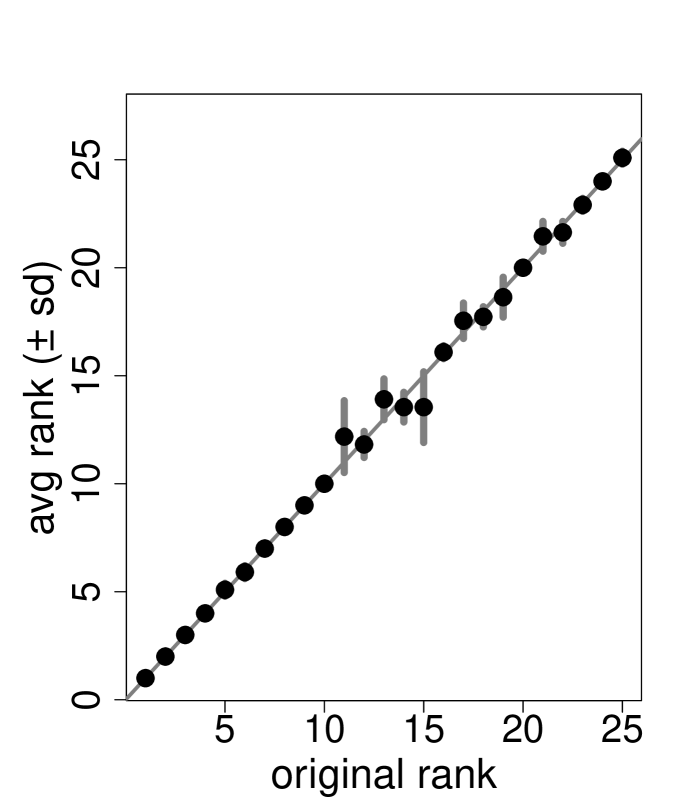
(b)

(c)

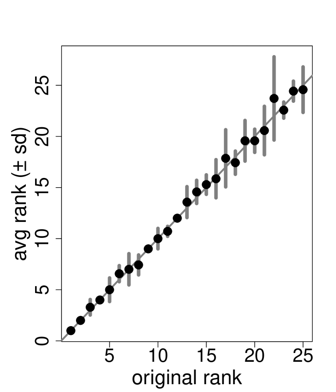
(d)

Fig. 4: (a) sLED applied on the M2c module with $c\in\{0.10,\cdots,0.30\}$. For each $c$, we visualize the number of genes with non-zero leverage, as well as the average and standard deviation of $p$-values in 10 repetitions, each using 1,000 permutations. (b) The average and standard deviation of ranks of the 25 primary genes when $c\in\{0.10,\cdots,0.30\}$, where ranks are based on the descending order of leverage. (c) sLED applied on 7 modules using $c=0.1$, including the original M2c module as well as 6 differently perturbed modules with sizes $\{1248,1357,1397,1452,1537,1708\}$. For each (perturbed) module, we visualize the number of genes with non-zero leverage, as well as the average and standard deviation of $p$-values in 10 repetitions, each using 1,000 permutations. (d) The average and standard deviation of ranks of the 25 primary genes when sLED is applied on the 7 (perturbed) modules using $c=0.1$, where ranks are based on the descending order of leverage.

4.3 Generalization to weighted adjacency matrices

Finally, we illustrate that sLED is not only applicable to testing differences in covariance matrices, but can also be applied to comparing general gene-gene “relationship” matrices. As an example, we consider the weighted adjacency matrix $A\in\mathbb{R}^{p\times p}$, defined as

$$A_{ij}=|R_{ij}|^{\beta}\,,\textrm{ for }1\leq i,j\leq p\,~{}\textrm{and some constant}~{}\beta>0\,,$$ (4.1)

where $R_{ij}$ is the Pearson correlation between gene $i$ and gene $j$, and the constant $\beta>0$ controls the density of the corresponding weighted gene network. The weighted adjacency matrix is widely used as a similarity measurement for gene clustering, and has been shown to yield genetic modules that are biologically more meaningful than using regular correlation matrices (Zhang and Horvath, 2005). Now the testing problem becomes

$$H_{0}:\tilde{D}=0\,\ \textrm{versus}\ H_{1}:\tilde{D}\neq 0\,,$$

where $\tilde{D}=\mathbb{E}(A_{control})-\mathbb{E}(A_{SCZ})$. While classical two-sample covariance testing procedures are inapplicable under this setting, sLED can be easily generalized to incorporate this scenario. Let $\hat{D}=A_{control}-A_{SCZ}$, then the same permutation procedure as described in Section 2.2 can be applied.

We explore the results of sLED for $\beta\in\{1,\,3,\,6.5,\,9\}$, corresponding to four different choices of weighted adjacency matrices. We choose the same sparsity parameter $c=0.1$ for sLED as in section 4.1, and with 1,000 permutations, the $p$-values are $0.020$, $0.001$, $0.002$, and $0.006$ for the 4 choices of $\beta$’s respectively. The latter three are significant at level $0.05$ after a Bonferroni correction.

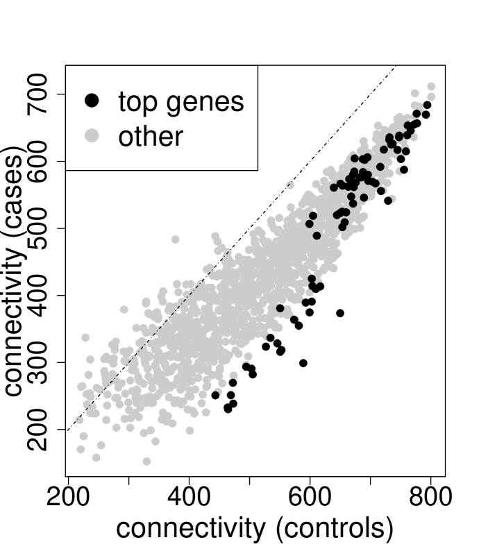
(a) $\beta=1$

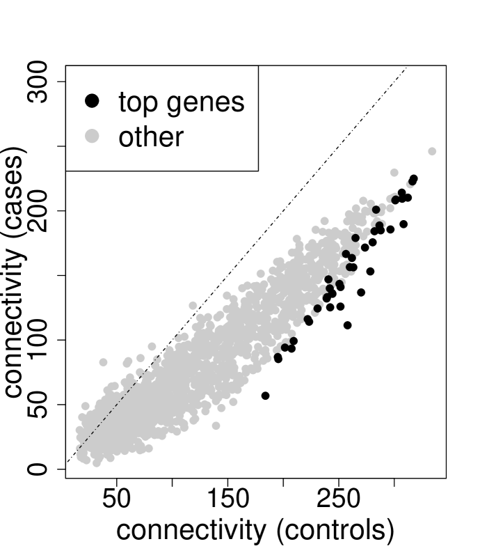
(b) $\beta=3$

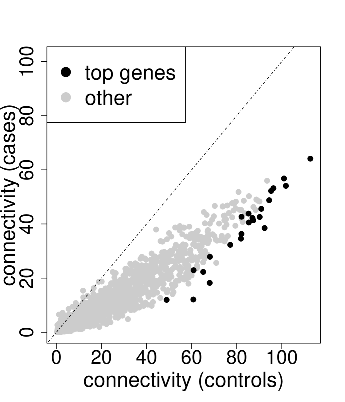
(c) $\beta=6.5$

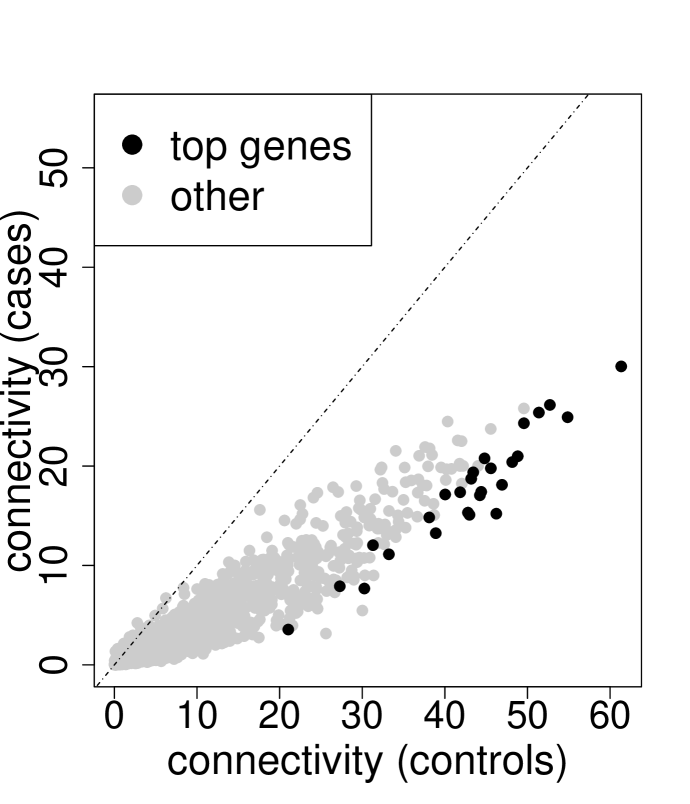
(d) $\beta=9$

Fig. 5: Connectivity in the M2c module for control and SCZ samples using weighted adjacency matrices with different $\beta$’s. The top genes detected by sLED with non-zero leverage are highlighted in black, and the auxiliary line $y=x$ is shown in each plot.

Interestingly, we find our results to be closely related to the connectivity of genes in the M2c module, where the connectivity of gene $i$ is defined as

$$k_{i}=\sum_{j\neq i}A_{ij}\,.$$

fig. 5 compares the gene connectivities between control and SCZ samples, where the top genes with non-zero leverage detected by sLED are highlighted. It is clear that the connectivity of genes is typically higher in control samples. Furthermore, as $\beta$ increases, the differences on highly connected genes are enlarged, and consistently, the top genes detected by sLED also concentrate more and more on these “hub” genes that are densely connected. These genes would have been missed by the covariance matrix test, but are now revealed using weighted adjacency matrices. A Gene Ontology (GO) enrichment analysis (Chen et al., 2013) highlights a different, although related, set of biological processes when $\beta=9$ versus $\beta=1$ (Table 3).

Table 3: Top 5 terms in Gene Ontology (GO) enrichment analysis on the top genes using weighted adjacency matrices with $\beta\in\{1,9\}$. The adjusted $p$-values are reported in parentheses.

$\beta=1$ $\beta=9$ 1 Positive regulation of cell development (4.4e-05) Synaptic transmission (5.6e-06) 2 Axon extension (4.6e-04) Energy reserve metabolic process (6.5e-06) 3 Regulation of cell morphogenesis involved in differentiation (1.7e-04) Divalent metal ion transport (4.1e-05) 4 Neuron projection extension (7.0e-04) Divalent inorganic cation transport (4.5e-05) 5 Positive regulation of nervous system development (6.5e-04) Calcium ion transport (2.8e-05)

5 Conclusion and discussion

In this paper, we propose sLED, a permutation test for two-sample covariance matrices under the high dimensional regime, which meets the need to understand the changes of gene interactions in complex human diseases. We prove that sLED achieves full power asymptotically; and in many biologically plausible settings, we verify by simulation studies that sLED outperforms many other existing methods. We apply sLED to a recently produced gene expression data set on Schizophrenia, and provide a list of 113 genes that show altered co-expression when brain samples from cases are compared to that from controls. We also reveal an interesting pattern of gene correlation change that has not been previously detected. The biological basis for this pattern is unclear. As more gene expression data become available, it will be interesting to validate these findings in an independent data set.

sLED can be applied to many other data sets for which signals are both sparse and weak. The performance is theoretically guaranteed for sub-Gaussian distributions, but we observe in simulation studies that sLED remains powerful when data has heavier tails. In terms of running time, on the 1,411 genes considered in this paper, sLED with 1,000 permutations takes 40 minutes using a single core on a computer equipped with an AMD Opteron(tm) Processor 6320 @ 2.8 GHz. When dealing with larger datasets, it is straightforward to parallelize the permutation procedure and further reduce the computation time.

Finally, we illustrate that sLED can be applied to a more general class of differential matrices between other gene-gene relationship matrices that are of practical interest. We show an example of comparing two weighted adjacency matrices and how this reveals novel insight on Schizophrenia. Although we have only stated the consistency results for testing covariance matrices, similar theoretical guarantee may be established for other relationship matrices as long as similar error bounds as in theorem 2 hold. This is a first step towards testing general high-dimensional matrices, and we leave a more thorough exploration in this direction to future work.

S1 Simulations

In this section, we present the remaining simulation results for comparing sLED with other existing methods, including Sfrob (Schott, 2007), Ustat (Li and Chen, 2012), Max (Cai, Liu and Xia, 2013), MBoot (Chang et al., 2016), and RProj (Wu and Li, 2015). As explained in Section 3 of the main paper, we use 100 permutations to compute the $p$-values for all methods, except for MBoot where 100 bootstrap repetitions are used, and we focus on comparing the empirical power.

The samples are generated by $X_{i}=\Sigma_{1}^{1/2}Z_{i}$ for $i=1,\cdots,n$, and $Y_{l}=\Sigma_{2}^{1/2}Z_{n+l}$ for $l=1,\cdots,m$, where $\{Z_{i}\}_{i=1,n+m}$ are independent $p$-dimensional random variables with $i.i.d.$ coordinates $Z_{ij}$, $j=1,\cdots,p$. For the different choices of $\Sigma_{1}$ and $\Sigma_{2}=\Sigma_{1}+D$, please refer to Section 3 in the main manuscript. We consider the following four distributions for $Z_{ij}$:

1. Standard Normal $N(0,1)$, which leads to multinomial Gaussian samples $X$ and $Y$.

2. Centralized Gamma distribution with $\alpha=4,\beta=0.5$ (i.e., the theoretical expectation $\alpha\beta=2$ is subtracted from $\Gamma(4,0.5)$ samples).

3. $t$-distribution with degrees of freedom 12.

4. Centralized Negative Binomial distribution with mean $\mu=2$ and dispersion parameter $\phi=2$ (i.e., the theoretical expectation $\mu=2$ is subtracted from NB$(2,2)$ samples).

Table S1 summarizes the empirical power under different covariance structures and differential matrices when $Z_{ij}$’s are sampled from $t$-distribution and centralized NB$(2,2)$. The results for standard Normal and centralized Gamma distributions are presented in Table 1 of the main manuscript. The smoothing parameter for sLED is set to be $\sqrt{R}=0.3\sqrt{p}$, and 100 random projections are used for Rproj. We also examine the sensitivity of sLED to the smoothing parameter in fig. S1, where $c$ is varied among $\{0.10,0.12,\cdots,0.30\}$ (recall that $\sqrt{R}=c\sqrt{p}$). We see that sLED achieves superior power to other approaches under most scenarios, and the results remain robust to many choices of $c$’s.

Table S1: Empirical power in 100 repetitions, where $n=m=100$, nominal level $\alpha=0.05$, and $Z_{ij}$’s are sampled from centralized Negative Binomial $(2,2)$ (top) and t-distribution with degrees of freedom 12 (bottom). Under each scenario, the largest power is highlighted.

$\mathbf{D}$ $\mathbf{\Sigma_{1}}$ Noisy diagonal Block diagonal Exp. decay WGCNA $\mathbf{p}$ 100 200 500 100 200 500 100 200 500 100 200 500 Centralized Negative Binomial Block Max 0.59 0.18 0.11 0.87 0.69 0.25 1.00 0.94 0.50 0.80 0.84 0.28 MBoot 0.47 0.12 0.07 0.80 0.60 0.16 0.99 0.82 0.33 0.72 0.73 0.17 Ustat 0.69 0.62 0.68 0.89 0.93 0.94 0.99 0.99 1.00 0.57 0.78 0.74 Sfrob 0.66 0.63 0.69 0.91 0.91 0.94 0.98 0.99 1.00 0.58 0.79 0.80 RProj 0.11 0.13 0.06 0.18 0.13 0.11 0.21 0.21 0.10 0.15 0.10 0.16 sLED 0.91 0.90 0.99 0.99 1.00 1.00 1.00 1.00 1.00 0.86 0.95 0.95 Spiked Max 0.04 0.07 0.06 0.60 0.20 0.10 0.93 0.82 0.25 0.93 0.41 0.06 MBoot 0.03 0.04 0.03 0.51 0.20 0.02 0.92 0.76 0.18 0.89 0.33 0.05 Ustat 0.25 0.12 0.03 0.82 0.35 0.13 0.98 0.94 0.72 0.36 0.12 0.03 Sfrob 0.25 0.11 0.03 0.85 0.35 0.12 0.98 0.96 0.69 0.40 0.12 0.06 RProj 0.08 0.07 0.02 0.31 0.17 0.10 0.35 0.17 0.06 0.58 0.17 0.13 sLED 0.22 0.04 0.08 0.97 0.68 0.16 0.99 1.00 1.00 0.96 0.48 0.13 T-distribution Block Max 0.22 0.15 0.12 0.88 0.73 0.23 1.00 0.85 0.27 0.97 0.40 0.15 MBoot 0.23 0.14 0.13 0.88 0.68 0.20 1.00 0.84 0.23 0.91 0.37 0.13 Ustat 0.53 0.63 0.74 0.97 0.93 0.96 1.00 0.99 1.00 0.75 0.67 0.84 Sfrob 0.52 0.63 0.71 0.97 0.93 0.97 1.00 0.99 0.99 0.74 0.67 0.76 RProj 0.08 0.13 0.11 0.28 0.12 0.02 0.28 0.19 0.08 0.17 0.13 0.06 sLED 0.95 0.99 0.99 0.99 1.00 1.00 1.00 1.00 1.00 0.95 0.97 0.92 Spiked Max 0.13 0.08 0.05 0.78 0.50 0.08 0.96 0.79 0.18 0.85 0.27 0.10 MBoot 0.12 0.07 0.03 0.78 0.49 0.07 0.97 0.77 0.11 0.83 0.32 0.13 Ustat 0.14 0.07 0.10 0.79 0.36 0.07 1.00 0.91 0.68 0.30 0.06 0.05 Sfrob 0.12 0.10 0.10 0.80 0.36 0.07 1.00 0.91 0.66 0.29 0.09 0.05 RProj 0.07 0.06 0.06 0.34 0.20 0.08 0.36 0.16 0.07 0.57 0.27 0.14 sLED 0.40 0.09 0.03 0.96 0.76 0.14 1.00 1.00 1.00 0.95 0.55 0.08

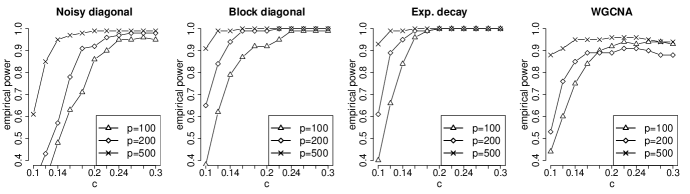
(a) $Z_{ij}\sim$ centralized $\Gamma(4,0.5)$.

(b) $Z_{ij}\sim$ centralized NB$(2,2)$.

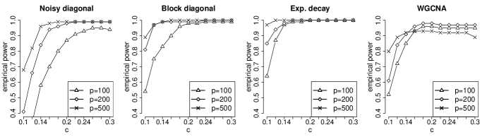
(c) $Z_{ij}\sim t(12)$.

Fig. S1: Empirical power of sLED in 100 repetitions using different smoothing parameters $\sqrt{R}=c\sqrt{p}$ for $c\in\{0.10,\cdots,0.30\}$, where $D$ has sparse block difference and $Z_{ij}$’s are sampled from different distributions.

S2 Proofs under $L_{1}$ constraints

In this section, we prove Theorems 1 to 3 for the asymptotic power of sLED.

Notation

For a set $\mathcal{A}$, let $|\mathcal{A}|$ be its cardinality, and $\mathcal{A}^{c}$ be its complement. For $Z=(Z_{1},\cdots Z_{N})=(X_{1},\cdots,X_{n},Y_{1},\cdots,Y_{m})$, we denote $Z_{ki}$ to be the $i$-th coordinate of the $k$-th sample $Z_{k}$, and

$$\begin{split}&\hat{\Sigma}=\frac{1}{N}\sum_{k=1}^{N}Z_{k}Z_{k}^{T}\,,\ \bar{Z}=\frac{1}{N}\sum_{k=1}^{N}Z_{k}=(\bar{Z}_{1},\cdots,\bar{Z}_{p})^{T}\,,\\ &m_{z}=||Z||_{\infty}\,,\ \overline{m}_{z}=||\bar{Z}||_{\infty}\,,\ \overline{m}_{z}^{(2q)}=\max_{1\leq i,j\leq p}\frac{1}{N}\sum_{k=1}^{N}Z_{ki}^{q}Z_{kj}^{q}\,,\,q=1,2\,.\end{split}$$

By Theorem 2 and Lemma 2, there exist some constants $C^{\prime},C^{\prime\prime}$ depending on $(\underline{c},\bar{c},\nu^{2},\delta)$, such that if $(n,p)$ are sufficiently large, with probability at least $1-\delta$,

$$||\hat{D}^{*}||_{\infty}\leq C^{\prime}\sqrt{\frac{\log p}{n}}\,,\ ||\hat{D}-D||_{\infty}\leq C^{\prime\prime}\sqrt{\frac{\log p}{n}}\,.$$

Then we apply Theorem 3 on both $\hat{D},-\hat{D}$ and $\hat{D}^{*},-\hat{D}^{*}$, and this together with assumption (A4) imply the desired conclusion with $C=C^{\prime}+C^{\prime\prime}$. ∎

• First, note that for $\forall\epsilon>0$,

  $$\mathbb{P}\left(||\hat{D}^{*}||_{\infty}>\epsilon\right)\leq\mathbb{P}\left(||\hat{\Sigma}_{1}^{*}-\hat{\Sigma}||_{\infty}>\frac{\epsilon}{2}\right)+\mathbb{P}\left(||\hat{\Sigma}_{2}^{*}-\hat{\Sigma}||_{\infty}>\frac{\epsilon}{2}\right)\,.$$ (S2.1)

  Now for any $\delta>0$ and constants $C_{1},C_{2}$, define

  $$\begin{split}\mathcal{A}=\left\{Z:\,m_{z}\leq C_{2}\sqrt{\log\left(\frac{C_{1}np}{\delta}\right)}\,,\,\overline{m}_{z}\leq C_{2}\sqrt{\frac{\log(C_{1}p/\delta)}{n}}\,,\,\overline{m}_{z}^{(2q)}\leq C_{2}\,,\,q=1,2\right\}.\end{split}$$

  By Lemma 2, there exist some constants $C_{1}$, $C_{2}$ depending on $(\underline{c},\bar{c},\nu^{2})$, such that if $(n,p)$ are sufficiently large, $\mathbb{P}\left(Z\not\in\mathcal{A}\right)\leq\delta/4$. Therefore, in order to show that

  $$\mathbb{P}\left(||\hat{\Sigma}_{1}^{*}-\hat{\Sigma}||_{\infty}>\frac{\epsilon}{2}\right)\leq\mathbb{P}\left(||\hat{\Sigma}_{1}^{*}-\hat{\Sigma}||_{\infty}>\frac{\epsilon}{2}\middle|Z\in\mathcal{A}\right)+\mathbb{P}\left(Z\not\in\mathcal{A}\right)\leq\frac{\delta}{2}\,,$$

  it suffices to show that given any $Z\in\mathcal{A}$, the conditional probability satisfies

  $$\mathbb{P}_{Z}\left(||\hat{\Sigma}_{1}^{*}-\hat{\Sigma}||_{\infty}>\frac{\epsilon}{2}\right)\leq\frac{\delta}{4}\,.$$ (S2.2)

  For any $1\leq i,j\leq p$, we first bound the $(i,j)$-th entry:

  $$\begin{split}\mathbb{P}_{Z}\left(|\hat{\Sigma}_{1,ij}^{*}-\hat{\Sigma}_{ij}|>\frac{\epsilon}{2}\right)\leq&\underbrace{\mathbb{P}_{Z}\left(\left|\frac{1}{n}\sum_{k=1}^{n}Z_{ki}^{*}Z_{kj}^{*}-\frac{1}{N}\sum_{k=1}^{N}Z_{ki}Z_{kj}\right|>\frac{\epsilon}{4}\right)}_{\Delta_{1}}+\\ &+\underbrace{\mathbb{P}_{Z}\left(\left|\bar{X}_{i}^{*}\bar{X}_{j}^{*}-\bar{Z}_{i}\bar{Z}_{j}\right|>\frac{\epsilon}{4}\right)}_{\Delta_{2}}\,,\end{split}$$

  where $\bar{X}_{i}^{*}=\frac{1}{n}\sum_{k=1}^{n}Z_{ki}^{*}$. Now we bound $\Delta_{1}$ and $\Delta_{2}$ separately.

  1. $\Delta_{1}$: Note that for any $(k,i,j)$,

     $$\left|Z_{ki}^{*}Z_{kj}^{*}\right|\leq(m_{z})^{2}\,,\ \textrm{var}_{Z}\left(Z_{ki}^{*}Z_{kj}^{*}\right)\leq\frac{1}{N}\sum_{l=1}^{N}Z_{li}^{2}Z_{lj}^{2}\leq\overline{m}_{z}^{(4)}\,.$$

     By Lemma 1, there exists a constant $C_{2}^{\prime}$ depending on $(C_{2},\nu^{2})$, such that if $(n,p)$ are sufficiently large,

     $$\Delta_{1}\leq 2\exp\left\{-\frac{n\epsilon^{2}/C_{2}^{\prime}}{1+\log(C_{1}np/\delta)\epsilon}\right\}.$$ (S2.3)

  2. $\Delta_{2}$: Note that

     $$\bar{X}_{i}^{*}\bar{X}_{j}^{*}-\bar{Z}_{i}\bar{Z}_{j}=(\bar{X}_{i}^{*}-\bar{Z}_{i})(\bar{X}_{j}^{*}-\bar{Z}_{j})+\bar{Z}_{j}(\bar{X}_{i}^{*}-\bar{Z}_{i})+\bar{Z}_{i}(\bar{X}_{j}^{*}-\bar{Z}_{j})\,,$$

     and for any $(k,i,j)$,

     $$|\bar{Z}_{i}|\leq\overline{m}_{z}\,,\ |Z_{ki}^{*}|\leq m_{z}\,,\ \textrm{var}_{Z}(Z_{ki}^{*})\leq\frac{1}{N}\sum_{l=1}^{N}Z_{li}^{2}\leq\overline{m}_{z}^{(2)}\,.$$

     Therefore,

     $$\Delta_{2}\leq 2\max_{i}\ \left[\mathbb{P}_{Z}\left(\left|\frac{1}{n}\sum_{k=1}^{n}Z_{ki}^{*}-\bar{Z}_{i}\right|>\sqrt{\frac{\epsilon}{8}}\right)+\mathbb{P}_{Z}\left(\left|\frac{1}{n}\sum_{k=1}^{n}Z_{ki}^{*}-\bar{Z}_{i}\right|>\frac{\epsilon}{16\overline{m}_{z}}\right)\right].$$

     Applying Lemma 1 on both terms, we know that there exists a constant $C_{2}^{\prime\prime}$ depending on $(C_{2},\nu^{2})$, such that if $(n,p)$ are sufficiently large,

     $$\begin{split}\Delta_{2}\leq&4\exp\left\{-\frac{n\epsilon/C_{2}^{\prime\prime}}{1+\sqrt{\log(C_{1}np/\delta)}\sqrt{\epsilon}}\right\}+\\ &\qquad 4\exp\left\{-\frac{n\epsilon^{2}/C_{2}^{\prime\prime}}{\frac{\log(C_{1}p/\delta)}{n}+\sqrt{\frac{\log(C_{1}p/\delta)\log(C_{1}np/\delta)}{n}}\epsilon}\right\}\,.\end{split}$$ (S2.4)

  Combining the results in eq. S2.3 and eq. S2.4, and note that $(\log p)^{3}=O(n)$ by assumption (A3), we have $\Delta_{1}\,,\Delta_{2}\leq\frac{\delta}{8}p^{-2}$ if $(n,p)$ are sufficiently large, as long as

  $$\epsilon\geq C^{\prime}\sqrt{\frac{\log(C_{1}p^{2}/\delta)}{n}}$$

  for some constant $C^{\prime}$ depending on $C_{2}^{\prime}$ and $C_{2}^{\prime\prime}$. Finally, eq. S2.2 follows from a union bound over $1\leq i,j\leq p$. Similar statement also holds for $||\hat{\Sigma}_{2}^{*}-\hat{\Sigma}||_{\infty}$ with sample size $m$, and the final result follows from eq. S2.1 and the fact that $\underline{c}n\leq m\leq\bar{c}n$. ∎

• 1. Note that a feasible solution of eq. 2.12 or eq. 2.14 always satisfies $||H||_{1}\leq R$, where $H=vv^{T}$ if using eq. 2.14. Then the result directly follows from the Hölder’s inequality:

     $$\textrm{tr}\left(\hat{D}H\right)\leq||\hat{D}||_{\infty}||H||_{1}\,.$$

  2. Let $v^{*}$ be the $R$-sparse leading eigenvector of $D$, then $||v^{*}||_{2}=1$ and $||v^{*}(v^{*})^{T}||_{1}=||v^{*}||_{1}^{2}\leq||v^{*}||_{0}=R$, so $v^{*}(v^{*})^{T}$ is feasible for eq. 2.12 and eq. 2.14. The result follows from

     $$\tilde{\lambda}_{1}^{R}(\hat{D})-\lambda_{1}^{R}(D)\geq(v^{*})^{T}\hat{D}v^{*}-(v^{*})^{T}Dv^{*}$$

     and $\left|(v^{*})^{T}(\hat{D}-D)v^{*}\right|\leq||\hat{D}-D||_{\infty}||v^{*}(v^{*})^{T}||_{1}$.

  ∎

S3 Proofs under $L_{0}$ constraints

In this section, we prove Theorem 4 for the power of sLED test under $L_{0}$-sparsity. We use the same notation as introduced in the beginning of Section S2. The proof of Theorem 4 is built on the following two theorems.

Theorem 5 (Permutation test statistic under $L_{0}$ constraint).

Let $\hat{D}^{*}$ be the permutation differential matrix as defined in eq. 2.9, and $\lambda_{1}^{R}(\hat{D}^{*})$ be the exact solution of eq. 2.7. Then under assumptions (A1)-(A2), for any $\delta>0$, there exist constants $C_{1},C_{2},C_{3}$ depending on $(\underline{c},\bar{c},\nu^{2})$, such that with probability at least $1-\delta$,

$$\lambda_{1}^{R}(\hat{D}^{*})\leq h(C_{1},C_{2},C_{3},t)\,,$$

where

$$h(C_{1},C_{2},C_{3},t)=C_{1}s\left[\log(C_{3}Np)+t\right]\frac{t}{N}+C_{2}\sqrt{\left(1+\frac{t+s\log(9ep/s)}{N}\right)\frac{t}{N}}\,,$$

and $s=\lfloor R\rfloor$, $t=s\log\left(9ep/s\right)+\log(1/\delta)$.

• Following Vershynin (2010), for an integer $s$, there exists a $\frac{1}{4}$-net $\mathcal{N}_{s}$ over the unit sphere $\mathbb{S}^{s-1}$, such that $|\mathcal{N}_{s}|\leq 9^{s}$, and for any matrix $A\in\mathbb{R}^{s\times s}$,

  $$\lambda_{1}(A)\leq 2\max_{v\in\mathcal{N}_{s}}v^{T}Av\,.$$

  Therefore, for any subset $\mathcal{S}\subseteq\{1,...,p\}$, let $\hat{D}_{\mathcal{S}}^{*}$ be the sub-matrix on $\mathcal{S}\times\mathcal{S}$, we have

  $$\lambda_{1}^{R}(\hat{D}^{*})=\lambda_{1}^{s}(\hat{D}^{*})=\max_{|\mathcal{S}|=s}\lambda_{1}\left(\hat{D}_{\mathcal{S}}^{*}\right)\leq 2\max_{|\mathcal{S}|=s}\,\max_{v\in\mathcal{N}_{s}}v^{T}\left(\hat{D}_{\mathcal{S}}^{*}\right)v\,.$$

  Moreover, for any given $v\in\mathcal{N}_{s}$ and subset $\mathcal{S}$, we can construct $u\in\mathbb{S}^{p-1}$ that is augmented from $v\in\mathbb{S}^{s-1}$ by adding zeros on coordinates in $\mathcal{S}^{c}$, then

  $$v^{T}\left(\hat{D}_{\mathcal{S}}^{*}\right)v=u^{T}\hat{D}^{*}u\,.$$

  We define the collection of such $u$’s to be

  $$\widetilde{\mathcal{N}}_{s}=\{u\in\mathbb{R}^{p}:||u||_{2}=1,\textrm{supp}(u)\subseteq\mathcal{S},|\mathcal{S}|=s,u(\mathcal{S})\in\mathcal{N}_{k}\}\,,$$

  where $u(\mathcal{S})$ is the sub-vector restricted on coordinates in $\mathcal{S}$, and we have

  $$\left|\widetilde{\mathcal{N}}_{s}\right|={p\choose s}\left|\mathcal{N}_{s}\right|\leq\left(\frac{9ep}{s}\right)^{s}\,.$$

  Next, we show that there exist constants $C_{1},C_{2},C_{3}$ depending on $(\underline{c},\bar{c},\nu^{2})$, such that

  $$\mathbb{P}\left(u^{T}\hat{D}^{*}u\geq h\left(\frac{C_{1}}{2},\frac{C_{2}}{2},C_{3},t\right)\right)\leq e^{-t},\,\forall t>0,\,\forall u\in\widetilde{N}_{s}\,.$$ (S3.1)

  Note that

  $$u^{T}\hat{D}^{*}u=\frac{1}{m}\sum_{l=(n+1)}^{N}\left(u^{T}Z_{l}^{*}\right)^{2}-\frac{1}{n}\sum_{k=1}^{n}\left(u^{T}Z_{k}^{*}\right)^{2}\,,$$

  and we define

  $$\gamma_{z}=\max_{u\in\widetilde{\mathcal{N}}_{s}}\max_{1\leq k\leq N}Z_{k}^{T}u\,,\ \bar{\gamma}_{z}^{(4)}=\max_{u\in\widetilde{\mathcal{N}_{s}}}\frac{1}{N}\sum_{k=1}^{N}(Z_{k}^{T}u)^{4}\,,$$

  and

  $$\mathcal{G}=\left\{Z:\gamma_{z}\leq C_{1}^{\prime}\sqrt{s}\sqrt{\log(C_{3}^{\prime}Np)+t}\,,\ \bar{\gamma}_{z}^{(4)}\leq C_{2}^{\prime}\left(1+\frac{t+s\log(9ep/s)}{N}\right)\right\}.$$

  Now for any $t>0$, by Lemma 3, there exist constants $C_{1}^{\prime},C_{2}^{\prime},C_{3}^{\prime}$ depending on $\nu^{2}$, such that

  $$\mathbb{P}\left(Z\in\mathcal{G}\right)\geq 1-\frac{e^{-t}}{2}\,.$$

  Therefore, in order to prove eq. S3.1, it suffices to show that given any $Z\in\mathcal{G}$, the conditional probability satisfies

  $$\mathbb{P}_{Z}\left(\frac{1}{m}\sum_{l=(n+1)}^{N}\left(u^{T}Z_{l}^{*}\right)^{2}-\frac{1}{n}\sum_{k=1}^{n}\left(u^{T}Z_{k}^{*}\right)^{2}\geq h\left(\frac{C_{1}}{2},\frac{C_{2}}{2},C_{3},t\right)\right)\leq\frac{e^{-t}}{2}\,.$$

  Note that given $Z\in\mathcal{G}$, $\left(u^{T}Z_{k}^{*}\right)^{2}$ satisfies

  $$\begin{split}&\max_{1\leq k\leq N}\left(u^{T}Z_{k}^{*}\right)^{2}\leq(\gamma_{z})^{2},\ \textrm{var}_{Z}\left[\left(u^{T}Z_{k}^{*}\right)^{2}\right]\leq\bar{\gamma}_{z}^{(4)}\,,\forall k=1,\cdots,N\,.\end{split}$$

  Therefore, by Lemma 1, there exist constants $C_{1},C_{2},C_{3}$ depending on $(\nu^{2},C_{1}^{\prime},C_{2}^{\prime},C_{3}^{\prime})$, such that

  $$\mathbb{P}_{Z}\left(\left|\frac{1}{n}\sum_{k=1}^{n}\left(u^{T}Z_{k}^{*}\right)^{2}-\frac{1}{N}\sum_{k=1}^{N}\left(u^{T}Z_{k}\right)^{2}\right|\geq h\left(\frac{C_{1}}{2},\frac{C_{2}}{2},C_{3},t\right)\right)\leq\frac{e^{-t}}{4}\,.$$

  Similar results also hold for $\frac{1}{m}\sum_{l=(n+1)}^{N}\left(u^{T}Z_{l}^{*}\right)^{2}$, and eq. S3.1 follows from $\underline{c}n\leq m\leq\bar{n}$. Finally, with a union bound over $\widetilde{\mathcal{N}}_{s}$, we have, for any $\delta>0$,

  $$\begin{split}\mathbb{P}\left(\lambda_{1}^{R}(\hat{D}^{*})>h(C_{1},C_{2},C_{3},t)\right)&\leq\sum_{u\in\widetilde{\mathcal{N}}_{s}}\mathbb{P}\left(u^{T}\hat{D}^{*}u>\frac{h(C_{1},C_{2},C_{3},t)}{2}\right)\\ &=\sum_{u\in\widetilde{\mathcal{N}}_{s}}\mathbb{P}\left(u^{T}\hat{D}^{*}u>h\left(\frac{C_{1}}{2},\frac{C_{2}}{2},C_{3},t\right)\right)\\ &\leq\left(\cfrac{9ep}{s}\right)^{s}e^{-t}=\delta\,,\end{split}$$

  where the last equality holds when $t=s\log(9ep/s)+\log(1/\delta)$. ∎

Theorem 6 (Signal under $L_{0}$ constraint).

Under assumptions (A1)-(A2), for any $\delta>0$, there exist constants $C_{1},C_{2}$, such that with probability at least $1-\delta$,

$$\lambda_{1}^{R}(\hat{D})\geq\lambda_{1}^{R}(D)-C_{1}\frac{\nu^{2}\log(2/\delta)}{n}-\sqrt{C_{2}\frac{\nu^{4}\log(2/\delta)}{n}}\,.$$

• Let $u_{0}\in B_{0}(R)=\{u:||u||_{2}=1,||u||_{0}\leq R\}$ such that $\lambda_{1}^{R}(D)=u_{0}^{T}Du_{0}$. Then

  $$\lambda_{1}^{R}(\hat{D})-\lambda_{1}^{R}(D)\geq u_{0}^{T}(\hat{D}-D)u_{0}\,.$$

  Therefore, it suffices to bound

  $$\left|u_{0}^{T}(\hat{D}-D)u_{0}\right|\leq\left|u_{0}^{T}(\hat{\Sigma}_{1}-\Sigma_{1})u_{0}\right|+\left|u_{0}^{T}(\hat{\Sigma}_{2}-\Sigma_{2})u_{0}\right|\,.$$

  For any $\epsilon>0$, note that $X_{k}^{T}u_{0}$ is sub-gaussian for $\forall k$, so by standard results (for example, Lemma 1 in Ravikumar et al. (2011)),

  $$\begin{split}\mathbb{P}\left(\left|u_{0}^{T}(\hat{\Sigma}_{1}-\Sigma_{1})u_{0}\right|>\epsilon\right)&=\mathbb{P}\left(\left|\frac{1}{n}\sum_{k=1}^{n}(X_{k}^{T}u_{0})^{2}-\mathbb{E}\left[(X_{1}^{T}u_{0})^{2}\right]\right|>\epsilon\right)\\ &\leq 2\exp\left\{-\frac{n\epsilon^{2}}{C_{1}^{\prime}\nu^{4}+C_{2}^{\prime}\nu^{2}\epsilon}\right\}\end{split}$$

  for some constants $C_{1}^{\prime},C_{2}^{\prime}$. The same arguments hold for $u_{0}^{T}(\hat{\Sigma}_{2}-\Sigma_{2})u_{0}$. ∎

Now we are able to state the proof for Theorem 4.

• By Theorem 5 and Theorem 6, together with assumption (A3’), we know that for any $\delta>0$, there exist some constants $C_{1},C_{2},C_{3}$ depending on $(\underline{c},\bar{c},\nu^{2},\delta)$, such that with probability at least $1-\delta$,

  $$\lambda_{1}^{R}(\hat{D}^{*})\leq C_{1}\sqrt{R\log(C_{2}p)/n}\,,\ \ \lambda_{1}^{R}(\hat{D})\geq\lambda_{1}^{R}(D)-C_{3}\sqrt{1/n}\,.$$

  The same arguments hold for $-\hat{D}^{*}$ and $-\hat{D}$. Therefore, under assumption (A4’) with some constant $C$ depending on $(\underline{c},\bar{c},\nu^{2},\delta)$, we have

  $$\mathbb{P}_{H_{1}}\left(T_{R}(\hat{D}^{*})>T_{R}(\hat{D})\right)\leq\delta.$$

  The remaining statement follows by setting $\delta=\alpha/2$ and applying the Hoeffding’s bound on the sample mean of Bernoulli random variables. ∎

S4 Lemmas

In this section, we state and prove the lemmas that are used in Section S2 and Section S3.

Lemma 1 (Bernstein inequality for sampling without replacement).

Let $\mathcal{Z}=\{z_{1},...,z_{N}\}$ be a finite set containing $N$ real numbers, and $(z_{1}^{*},...,z_{n}^{*})$ be $i.i.d.$ random variables that are drawn without replacement from $\mathcal{Z}$. Let

$$\bar{z}=\max_{1\leq i\leq N}|z_{i}|\,,\ \mu_{z}=\frac{1}{N}\sum_{i=1}^{N}z_{i}\,,\ \sigma_{z}^{2}=\frac{1}{N}\sum_{i=1}^{N}(z_{i}-\mu_{z})^{2}\,,$$

then for any $\epsilon>0$,

$$\mathbb{P}\left(\left|\frac{1}{n}\sum_{i=1}^{n}z_{i}^{*}-\mu_{z}\right|\geq\epsilon\right)\leq 2\exp\left\{-\frac{n\epsilon^{2}}{2\sigma_{z}^{2}+\frac{4}{3}\bar{z}\epsilon}\right\}\,.$$

As a consequence, for any $t>0$,

$$\mathbb{P}\left(\left|\frac{1}{n}\sum_{i=1}^{n}z_{i}^{*}-\mu_{z}\right|>\frac{4\bar{z}}{3}\frac{t}{n}+\sqrt{2\sigma_{z}^{2}\frac{t}{n}}\right)\leq 2e^{-t}\,.$$

• See Proposition 1.4 in Bardenet et al. (2015). ∎

Lemma 2 (Sub-gaussian tail bound).

Under assumptions (A1)-(A2), for $\forall\delta>0$, there exist constants $C_{1},C_{2}$ depending on $(\underline{c},\bar{c},\nu^{2})$, such that if $(n,p)$ are sufficiently large, with probability at least $1-\delta$,

1. $||\hat{\Sigma}_{q}-\Sigma_{q}||_{\infty}\leq C_{2}\sqrt{\frac{\log(C_{1}p^{2}/\delta)}{N}}$ for $q=1,2$. As a consequence,

   $$||\hat{D}-D||_{\infty}\leq 2C_{2}\sqrt{\frac{\log(C_{1}p^{2}/\delta)}{N}}\,.$$

2. $\overline{m}_{z}\leq C_{2}\sqrt{\frac{\log(C_{1}p/\delta)}{N}}$. This together with (i) imply that

   $$\overline{m}_{z}^{(2)}\leq 2\nu^{2}+2C_{2}\sqrt{\frac{\log(C_{1}p^{2}/\delta)}{N}}\,.$$

3. $m_{z}\leq C_{2}\sqrt{\log(C_{1}Np/\delta)}$.

4. $\overline{m}_{z}^{(4)}\leq C_{2}\left[1+\frac{\log(C_{1}p^{2}/\delta)}{N}\right]$.

• 1. See for example, Lemma 12 in Yuan (2010).

  2. The first part is standard Hoeffding’s bound on $\frac{1}{N}\sum_{k=1}^{N}Z_{ki}$, with a union bound over $1\leq i\leq p$. The second part follows from

     $$\overline{m}_{z}^{(2)}\leq\max\{||\hat{\Sigma}_{1}||_{\infty},||\hat{\Sigma}_{2}||_{\infty}\}+(\overline{m}_{z})^{2}\,.$$

  3. By Markov inequality, $\forall\epsilon,t>0$,

     $$\begin{split}\mathbb{P}\left(\max_{k,i}Z_{ki}>\epsilon\right)&\leq e^{-t\epsilon}\mathbb{E}\left[e^{t\max_{k,i}Z_{ki}}\right]=e^{-t\epsilon}\mathbb{E}\left[\max_{k,i}e^{tZ_{ki}}\right]\\ &\leq e^{-t\epsilon}\sum_{k=1}^{N}\sum_{i=1}^{p}\mathbb{E}\left[e^{tZ_{ki}}\right]\leq Np\cdot e^{-t\epsilon+\frac{t^{2}\nu^{2}}{2}}\,.\end{split}$$

     Finally, take $t=\frac{\epsilon}{\nu^{2}}$, and note that similar arguments hold for $-Z_{ki}$.

  4. For any given $(i,j)$, let $W_{k}=Z_{ki}^{2}Z_{kj}^{2}$, and define its cumulant generating function

     $$\Psi_{k}(\theta)=\log\mathbb{E}\left[e^{\theta(W_{k}-\mathbb{E}(W_{k}))}\right]\,.$$

     Note that $\Psi_{1}=\cdots=\Psi_{n}$ and $\Psi_{n+1}=\cdots=\Psi_{n+m}$. By Markov inequality, for any $t,\theta>0$,

     $$\mathbb{P}\left(\left|\frac{1}{n}\sum_{k=1}^{n}W_{k}-\mathbb{E}(W_{1})\right|>t\right)\leq 2\exp\left\{-n\theta t+n\Psi(\theta)\right\}\,,$$ (S4.1)

     where $\Psi(\theta)=\max\{\Psi_{1}(\theta),\Psi_{n+1}(\theta)\}$ is an upper bound of the cumulant generating functions. Since $Z_{ki},Z_{kj}$ are sub-gaussian, there exists a small constant $\theta_{0}\neq 0$, such that $\Psi(\theta_{0})<\infty$. Plugging in $\theta_{0}$ to eq. S4.1, we know that with probability at least $1-\frac{\delta}{2}p^{-2}$,

     $$\frac{1}{n}\sum_{k=1}^{n}W_{k}-\mathbb{E}(W_{1})\leq\frac{\log(4p^{2}/\delta)}{n\theta_{0}}+\frac{\Psi(\theta_{0})}{\theta_{0}}\,.$$

     The same arguments also hold for $\frac{1}{m}\sum_{k=(n+1)}^{n+m}W_{k}-\mathbb{E}(W_{n+1})$. Then the final result follows from a union bound over $(i,j)$ and the fact that $\mathbb{E}(W_{k})\leq C\nu^{4}$ for some constant $C$.

  ∎

Lemma 3.

Under the same conditions as Theorem 5, let $\widetilde{\mathcal{N}}_{s}\subseteq B_{0}(s)=\{u\in\mathbb{R}^{p}:||u||_{2}=1,||u||_{0}\leq s\}$ be a finite set such that $\left|\widetilde{\mathcal{N}}_{s}\right|<\infty$. Define

$$\gamma_{z}=\max_{u\in\widetilde{\mathcal{N}}_{s}}\max_{1\leq k\leq N}Z_{k}^{T}u\,,\ \bar{\gamma}_{z}^{(4)}=\max_{u\in\widetilde{\mathcal{N}}_{s}}\frac{1}{N}\sum_{k=1}^{N}(Z_{k}^{T}u)^{4}\,.$$

Then for any $t>0$, there exist constants $C_{1},C_{2},C_{3}$ depending on $\nu^{2}$, such that with probability at least $1-e^{-t}$,

$$\gamma_{z}\leq C_{1}\sqrt{s}\sqrt{\log(C_{3}Np)+t}\,,\ \bar{\gamma}_{z}^{(4)}\leq C_{2}\left[1+\frac{t+\log\left|\widetilde{\mathcal{N}}_{s}\right|}{N}\right]\,.$$

• Let $m_{z}=||Z||_{\infty}=\max_{1\leq k\leq N,1\leq j\leq p}Z_{kj}$, and note that

  $$\gamma_{z}=\max_{u\in\widetilde{\mathcal{N}}_{s}}\max_{1\leq k\leq N}Z_{k}^{T}u\leq m_{z}\cdot\max_{u\in\widetilde{\mathcal{N}}_{s}}\sum_{j=1}^{s}u_{j}\leq m_{z}\sqrt{s}\,.$$

  Then the first result follows from Lemma 2.

  Next, for any $u\in\widetilde{\mathcal{N}}_{s}$, denote $W_{u,k}=(Z_{k}^{T}u)^{4}$, with cumulant generating function

  $$\Psi_{k}(\theta)=\log\mathbb{E}\left[e^{\theta\left[W_{u,k}-\mathbb{E}(W_{u,k})\right]}\right]\,.$$

  Note that $\Psi_{1}=\cdots=\Psi_{n}$ and $\Psi_{n+1}=\cdots=\Psi_{n+m}$. Then for any $\epsilon,\theta>0$, by Markov inequality,

  $$\mathbb{P}\left(\frac{1}{N}\sum_{k=1}^{N}\left(W_{u,k}-\mathbb{E}(W_{u,k})\right)>\epsilon\right)\leq\exp\left\{-N\theta\epsilon+N\Psi(\theta)\right\}\,,$$ (S4.2)

  where $\Psi(\theta)=\max\{\Psi_{1}(\theta),\Psi_{n+1}(\theta)\}$. Note that $\{W_{u,k}\}_{k=1,...,N}$ are sub-gaussian, so there exists a small constant $\theta_{0}\neq 0$, such that $\Psi(\theta_{0})<\infty$. Therefore, plugging $\theta_{0}$ into eq. S4.2, we know that with probability at least $1-e^{-t}/|\widetilde{\mathcal{N}}_{s}|$,

  $$\frac{1}{N}\sum_{k=1}^{N}\left(W_{u,k}-\mathbb{E}(W_{u,k})\right)\leq\frac{t+\log\left|\widetilde{\mathcal{N}}_{s}\right|}{N\theta_{0}}+\frac{\Psi(\theta_{0})}{\theta_{0}}\,.$$

  Finally, the desired result follows from a union bound over $u\in\widetilde{\mathcal{N}}_{s}$ and the fact that $\mathbb{E}(W_{u,k})\leq C\nu^{4}$ for some constant $C$. ∎

References

- Anderson et al. (1958) Anderson, T. W., Anderson, T. W., Anderson, T. W. and Anderson, T. W. (1958). An introduction to multivariate statistical analysis 2. Wiley New York.
- Bai et al. (2009) Bai, Z., Jiang, D., Yao, J.-F. and Zheng, S. (2009). Corrections to LRT on large-dimensional covariance matrix by RMT. The Annals of Statistics 3822–3840.
- Bardenet et al. (2015) Bardenet, R., Maillard, O.-A. et al. (2015). Concentration inequalities for sampling without replacement. Bernoulli 21 1361–1385.
- Berthet and Rigollet (2013) Berthet, Q. and Rigollet, P. (2013). Optimal detection of sparse principal components in high dimension. The Annals of Statistics 41 1780–1815.
- Cai, Liu and Xia (2013) Cai, T., Liu, W. and Xia, Y. (2013). Two-sample covariance matrix testing and support recovery in high-dimensional and sparse settings. Journal of the American Statistical Association 108 265–277.
- Cai and Zhang (2015) Cai, T. T. and Zhang, A. (2015). Inference on High-dimensional Differential Correlation Matrix. Journal of Multivariate Analysis 142 107–126.
- Chang et al. (2016) Chang, J., Zhou, W., Zhou, W.-X. and Wang, L. (2016). Comparing Large Covariance Matrices under Weak Conditions on the Dependence Structure and its Application to Gene Clustering. arXiv preprint arXiv:1505.04493v3.
- Chen et al. (2013) Chen, E. Y., Tan, C. M., Kou, Y., Duan, Q., Wang, Z., Meirelles, G. V., Clark, N. R. and Ma’ayan, A. (2013). Enrichr: interactive and collaborative HTML5 gene list enrichment analysis tool. BMC Bioinformatics 14 128.
- International Schizophrenia Consortium et al. (2009) International Schizophrenia Consortium, Purcell, S. M., Wray, N. R., Stone, J. L., Visscher, P. M., O’Donovan, M. C., Sullivan, P. F. and Sklar, P. (2009). Common polygenic variation contributes to risk of schizophrenia and bipolar disorder. Nature 460 748-52.
- d’Aspremont et al. (2007) d’Aspremont, A., El Ghaoui, L., Jordan, M. I. and Lanckriet, G. R. (2007). A direct formulation for sparse PCA using semidefinite programming. SIAM review 49 434–448.
- Diniz et al. (2012) Diniz, L. P., Almeida, J. C., Tortelli, V., Vargas Lopes, C., Setti-Perdigão, P., Stipursky, J., Kahn, S. A., Romão, L. F., de Miranda, J., Alves-Leon, S. V., de Souza, J. M., Castro, N. G., Panizzutti, R. and Gomes, F. C. A. (2012). Astrocyte-induced synaptogenesis is mediated by transforming growth factor β signaling through modulation of D-serine levels in cerebral cortex neurons. J Biol Chem 287 41432-45.
- Fromer et al. (2016) Fromer, M., Roussos, P., Sieberts, S. K., Johnson, J. S., Kavanagh, D. H., Perumal, T. M., Ruderfer, D. M., Oh, E. C., Topol, A., Shah, H. R., Klei, L. L., Kramer, R., Pinto, D., Gümüş, Z. H., Cicek, A. E., Dang, K. K., Browne, A., Lu, C., Xie, L., Readhead, B., Stahl, E. A., Xiao, J., Parvizi, M., Hamamsy, T., Fullard, J. F., Wang, Y.-C., Mahajan, M. C., Derry, J. M. J., Dudley, J. T., Hemby, S. E., Logsdon, B. A., Talbot, K., Raj, T., Bennett, D. A., De Jager, P. L., Zhu, J., Zhang, B., Sullivan, P. F., Chess, A., Purcell, S. M., Shinobu, L. A., Mangravite, L. M., Toyoshiba, H., Gur, R. E., Hahn, C.-G., Lewis, D. A., Haroutunian, V., Peters, M. A., Lipska, B. K., Buxbaum, J. D., Schadt, E. E., Hirai, K., Roeder, K., Brennand, K. J., Katsanis, N., Domenici, E., Devlin, B. and Sklar, P. (2016). Gene expression elucidates functional impact of polygenic risk for schizophrenia. Nat Neurosci 19 1442-1453.
- Gu et al. (2015) Gu, X., Li, A., Liu, S., Lin, L., Xu, S., Zhang, P., Li, S., Li, X., Tian, B., Zhu, X. and Wang, X. (2015). MicroRNA124 Regulated Neurite Elongation by Targeting OSBP. Mol Neurobiol.
- Johnstone and Lu (2009) Johnstone, I. M. and Lu, A. Y. (2009). On consistency and sparsity for principal components analysis in high dimensions. Journal of the American Statistical Association 104 682–693.
- Jolliffe, Trendafilov and Uddin (2003) Jolliffe, I. T., Trendafilov, N. T. and Uddin, M. (2003). A modified principal component technique based on the LASSO. Journal of computational and Graphical Statistics 12 531–547.
- Li and Chen (2012) Li, J. and Chen, S. X. (2012). Two sample tests for high-dimensional covariance matrices. The Annals of Statistics 40 908–940.
- McGrath et al. (2008) McGrath, J., Saha, S., Chant, D. and Welham, J. (2008). Schizophrenia: a concise overview of incidence, prevalence, and mortality. Epidemiol Rev 30 67-76.
- Schizophrenia Working Group of the Psychiatric Genomics Consortium (2014) Schizophrenia Working Group of the Psychiatric Genomics Consortium (2014). Biological insights from 108 schizophrenia-associated genetic loci. Nature 511 421-7.
- Owen, Sawa and Mortensen (2016) Owen, M. J., Sawa, A. and Mortensen, P. B. (2016). Schizophrenia. Lancet.
- Oymak et al. (2015) Oymak, S., Jalali, A., Fazel, M., Eldar, Y. C. and Hassibi, B. (2015). Simultaneously Structured Models with Application to Sparse and Low-rank Matrices. IEEE Transactions on Information Theory 61 2886–2908.
- Purcell et al. (2014) Purcell, S. M., Moran, J. L., Fromer, M., Ruderfer, D., Solovieff, N., Roussos, P., O’Dushlaine, C., Chambert, K., Bergen, S. E., Kähler, A., Duncan, L., Stahl, E., Genovese, G., Fernández, E., Collins, M. O., Komiyama, N. H., Choudhary, J. S., Magnusson, P. K. E., Banks, E., Shakir, K., Garimella, K., Fennell, T., DePristo, M., Grant, S. G. N., Haggarty, S. J., Gabriel, S., Scolnick, E. M., Lander, E. S., Hultman, C. M., Sullivan, P. F., McCarroll, S. A. and Sklar, P. (2014). A polygenic burden of rare disruptive mutations in schizophrenia. Nature 506 185-90.
- Ravikumar et al. (2011) Ravikumar, P., Wainwright, M. J., Raskutti, G., Yu, B. et al. (2011). High-dimensional covariance estimation by minimizing 1-penalized log-determinant divergence. Electronic Journal of Statistics 5 935–980.
- Schott (2007) Schott, J. R. (2007). A test for the equality of covariance matrices when the dimension is large relative to the sample sizes. Computational Statistics & Data Analysis 51 6535–6542.
- Shen and Huang (2008) Shen, H. and Huang, J. Z. (2008). Sparse principal component analysis via regularized low rank matrix approximation. Journal of multivariate analysis 99 1015–1034.
- Srivastava and Yanagihara (2010) Srivastava, M. S. and Yanagihara, H. (2010). Testing the equality of several covariance matrices with fewer observations than the dimension. Journal of Multivariate Analysis 101 1319–1329.
- Székely and Rizzo (2013) Székely, G. J. and Rizzo, M. L. (2013). Energy statistics: A class of statistics based on distances. Journal of Statistical Planning and Inference 143 1249 - 1272.
- Vershynin (2010) Vershynin, R. (2010). Introduction to the non-asymptotic analysis of random matrices. arXiv preprint arXiv:1011.3027.
- Vu et al. (2013) Vu, V. Q., Cho, J., Lei, J. and Rohe, K. (2013). Fantope projection and selection: A near-optimal convex relaxation of sparse PCA. In Advances in Neural Information Processing Systems 26 2670–2678.
- Witten, Tibshirani and Hastie (2009) Witten, D. M., Tibshirani, R. and Hastie, T. (2009). A penalized matrix decomposition, with applications to sparse principal components and canonical correlation analysis. Biostatistics 10 515–534.
- Wu and Li (2015) Wu, T.-L. and Li, P. (2015). Tests for High-Dimensional Covariance Matrices Using Random Matrix Projection. arXiv preprint arXiv:1511.01611.
- Yu et al. (2014) Yu, C.-Y., Gui, W., He, H.-Y., Wang, X.-S., Zuo, J., Huang, L., Zhou, N., Wang, K. and Wang, Y. (2014). Neuronal and astroglial TGFβ-Smad3 signaling pathways differentially regulate dendrite growth and synaptogenesis. Neuromolecular Med 16 457-72.
- Yuan (2010) Yuan, M. (2010). High dimensional inverse covariance matrix estimation via linear programming. The Journal of Machine Learning Research 11 2261–2286.
- Zhang and Horvath (2005) Zhang, B. and Horvath, S. (2005). A general framework for weighted gene co-expression network analysis. Statistical applications in genetics and molecular biology 4 Article17.
- Zou, Hastie and Tibshirani (2006) Zou, H., Hastie, T. and Tibshirani, R. (2006). Sparse principal component analysis. Journal of computational and graphical statistics 15 265–286.