A Fast Order-Based Approach for Core Maintenance

Abstract

Graphs have been widely used in many applications such as social networks, collaboration networks, and biological networks. One important graph analytics is to explore cohesive subgraphs in a large graph. Among several cohesive subgraphs studied, $k$-core is one that can be computed in linear time for a static graph. Since graphs are evolving in real applications, in this paper, we study core maintenance which is to reduce the computational cost to compute $k$-cores for a graph when graphs are updated from time to time dynamically. We identify drawbacks of the existing efficient algorithm, which needs a large search space to find the vertices that need to be updated, and has high overhead to maintain the index built, when a graph is updated. We propose a new order-based approach to maintain an order, called $k$-order, among vertices, while a graph is updated. Our new algorithm can significantly outperform the state-of-the-art algorithm up to 3 orders of magnitude for the 11 large real graphs tested. We report our findings in this paper.

I Introduction

Due to the ubiquity of graph data in different applications, graph analytics has attracted much attention from both research and industry communities. One major issue in graph analytics is to identify cohesive subgraphs in the graphs, such as $k$-cores [4], $k$-trusses [15], cliques, $n$-cliques, and $n$-clans [6]. Among them, a $k$-core is defined as the maximal subgraph of an undirected graph $G$ such that all vertices in the subgraph have degree of at least $k$. For each vertex $v$ in $G$, the core number of $v$ is defined as the maximum $k$ such that $v$ is contained in the $k$-core of $G$. $k$-cores can be computed in linear time, whereas the time complexity for $k$-trusses is $\mathcal{O}(m^{1.5})$ [15], and cliques, $n$-cliques, and $n$-clans are NP-hard problems [6]. Due to its linear computability, $k$-cores have been widely used in many real-world applications, including graph visualization [3], community search [11], system structure analysis [17], network topology analysis [2] and so on. There are many works studying how to compute the core number for every vertex in a static graph efficiently. Such a problem is known as a core decomposition problem [4, 5, 10, 12, 16].

However, in many real-world applications, such as online social network, collaboration network, and Internet, graphs are evolving where vertices/edges will be inserted/removed over time dynamically. There are increasing interests to study how to handle dynamic graphs. To mention a few, [18] proposes a general technique to maintain a class of $2$-hop labels for reachability queries in dynamic graphs; [8] presents a scalable algorithm to maintain approximate densest subgraphs in the dynamic graph model with provable guarantee; [9] solves the problem of incrementally maintaining the matches to a query pattern when updates to the data graph are allowed. The problem of maintaining core numbers for an evolving graph is called core maintenance. In brief, after inserting an edge into or removing an edge from an undirected graph $G=(V,E)$, the problem is how to update the core numbers for the vertices that need to be updated. There are two important tasks in a core maintenance algorithm. First, it needs to identify the set of vertices whose core numbers need to be updated when an edge is inserted/removed. Such a set is denoted as $V^{*}$. Second, it recomputes the core numbers for the vertices in $V^{*}$. In order to achieve high efficiency, an index is used and the index needs to be maintained accordingly. In this paper, we study efficient in-memory core maintenance. Ideally, a good core maintenance algorithm should satisfy the following three criteria: (a) a small performance variation among edge updates, (b) a small cost for identifying $V^{*}$, and (c) a small cost for updating the index.

Figure 1: The distribution of the number of vertices visited: the traversal insertion algorithm (left bar) vs our new order-based insertion algorithm (right bar)

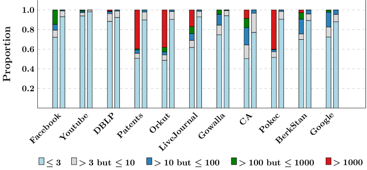
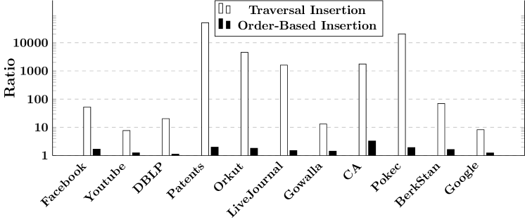
Sariyüce et al. in [13] propose an algorithm, called traversal algorithm, which is the state-of-the-art approach for core maintenance. The traversal algorithm searches for $V^{*}$ only in a local region near the edge inserted/removed. Therefore, it is much faster than recomputing core numbers from scratch. However, the traversal algorithm has drawbacks. First, it shows high variation in terms of performance when edges are inserted into a graph. We conduct testings to insert 100,000 edges into 11 real graphs tested (Table I). For each edge inserted, the algorithm visits some vertices, denoted as $V^{\prime}$, in order to identify $V^{*}$. We show the distribution of the size of $V^{\prime}$ over all the 100,000 edges inserted in Figure 1. As shown in Figure 1, for each of the 11 real graphs tested, there are two bars. The left bar is by the traversal insertion algorithm, whereas the right bar is by our new order-based insertion algorithm. A bar shows the corresponding proportion of edges inserted for different $|V^{\prime}|$. For example, for a large proportion of the 100,000 edges inserted, both our algorithm and the traversal algorithm only visit up to 3 vertices. However, the traversal insertion algorithm needs to visit more than 1,000 vertices for a non-small proportion of edge insertions, as shown by certain left bars. Our order-based algorithm only needs to visit up to 100 vertices for any of the 11 graphs, showing small performance variation. Second, we show the ratio of the size of the set of vertices visited ($|V^{\prime}|$) to the size of the set of vertices ($|V^{*}|$) that need to be updated, i.e., $\frac{\textnormal{sum of }|V^{\prime}|\textnormal{ over all insertions}}{\textnormal{sum of }|V^{*}|\textnormal{ over all insertions}}$ for the 100,000 edge insertions over each of the same 11 graphs in Figure 2. For the traversal insertion algorithm, the ratio is at least $7$ and can be up to 10,000 for $\mathsf{Patents}$ and $\mathsf{Pokec}$. It suggests the deficiency of the traversal insertion algorithm, even though it is the state-of-the-art. In contrast, for our new insertion algorithm, the ratios are below $4$ for all graphs tested and can be down to about 1. Third, for the traversal algorithm, the cost to maintain the index is high. The traversal algorithm maintains a value ${\mathsf{pcd}}(v)$, called the pure-core degree of $v$, for each $v$. Here, ${\mathsf{pcd}}(v)$ is computed from the core numbers of all vertices in the $2$-hops neighborhood of $v$. Therefore, if the core number of a vertex changes, a large number of vertices may have their ${\mathsf{pcd}}$ values to be updated, which incurs high cost. We will revisit the traversal algorithm in details in Section IV.

Figure 2: Ratio of number of vertices visited: the traversal insertion algorithm vs our new order-based insertion algorithm

The main contributions of this work are summarized below. First, we identify the deficiency of the state-of-the-art traversal algorithm [13] for core maintenance. Second, we propose new order-based in-memory algorithms for core maintenance: $\mathsf{OrderInsert}$ for edge insertion and $\mathsf{OrderRemoval}$ for edge removal. Note that, in this work, we do not consider vertex insertion/removal, since they can be simulated by a sequence of edge insertions and removals [11, 13, 16]. The main idea behind our new order-based algorithms is that we explicitly maintain a $k$-order among vertices such that $u\preceq v$ for every two vertices in a graph $G$. Here, a $k$-order, $(v_{1},v_{2},\ldots,v_{n})$, for every vertex $v_{i}$ in a graph $G$, is an instance of all the possible vertex sequences produced by a core decomposition algorithm [4]. In other words, there are many possible vertex sequences produced by a core decomposition algorithm, and we ensure the $k$-order under maintenance is one of them at any time for any evolving graph $G$. The transitivity holds. That is, $v_{h}\preceq v_{j}$ if $v_{h}\preceq v_{i}$ and $v_{i}\preceq v_{j}$. Given a $k$-order maintained for $G$, when an edge is inserted/removed, we maintain the $k$-order for the new $G$ with the edge inserted/removed. Third, we have conducted extensive performance studies, and show that we can achieve high efficiency up to 2,083 times faster than the traversal insertion algorithm.

The rest of this paper is organized as follows. We discuss the related work in Section II. We give the preliminaries in Section III, and review the traversal insertion/removal algorithm in Section IV. We discuss our new order-based algorithm, namely, $\mathsf{OrderInsert}$ and $\mathsf{OrderRemoval}$, in Section V, and give some implementation details in Section VI. We conduct extensive performance studies, and report the results in Section VII, and conclude this work in Section VIII.

II Related Work

Identifying cohesive subgraphs is an important problem in graph analytics. Common cohesive subgraphs are clique (maximal clique), $k$-plex, $n$-clique, $n$-clan [6], $k$-truss [15], $k$-core [4] and so on, among which $k$-core is the only one known to have a linear algorithm. We review the related work on computing $k$-core (core decomposition) and maintaining $k$-core (core maintenance) respectively below.

Core Decomposition: The core decomposition is to efficiently compute for each vertex its core number. [4] proposes an in-memory linear algorithm ($\mathcal{O}(m+n)$). Their algorithm uses a bottom-up process in which $k$-cores are computed in the order of $1$-core, $2$-core, $3$-core, $\cdots$. To process graphs that can not reside in the memory, [5] proposes an external algorithm, which runs in a top-down manner such that the whole graph does not need to be loaded to memory to compute higher cores. [16] proposes a new semi-external algorithm, which assumes that the memory has at least $\Omega(n)$ size and can maintain a small constant amount of information for each vertex in memory. [12] considers core decomposition under a distributed setting. [10] investigates core decomposition of large graphs using $\mathsf{GraphChi}$, $\mathsf{WebGraph}$, and external model, and compares their performance in a single PC.

Core Maintenance: Given a large graph, it takes high computational cost to recompute core numbers for vertices when some edges are inserted/removed, even though there exist linear algorithms. The core maintenance is to maintain core numbers efficiently when edges and vertices are inserted/removed. Since the insertions and removals of vertices can be simulated by a sequence of edge insertions and removals, all existing works [11, 13, 16, 1] consider only edge updates. The key issue is how to efficiently identify the set of vertices, denoted as $V^{*}$, whose core numbers need to be updated, around the edge inserted/removed. Recently, [11] and [13] independently found that, when an edge is inserted or removed, the induced subgraph of $V^{*}$ is connected and moreover, $V^{*}$ resides in the subcore which the edge is in. Based on this observation, [13] proposes algorithms that are linear in the size of the subcore, whereas [11] proposes a quadratic algorithm. Among the algorithms proposed in [13], the traversal algorithm is the state-of-the-art for core maintenance. We will revisit the traversal algorithm later, and show that we can significantly improve the efficiency when a graph can be held in memory. A semi-external algorithm for core maintenance is proposed in [16] to reduce I/O cost; but it is not optimized for CPU time. The algorithm proposed by [1] is similar to the $\mathsf{SubCore}$ algorithm of [13] but is less efficient due to weaker bounds.

III The Preliminaries

Let $G=(V,E)$ be an undirected graph, where $V(G)$ denotes the set of vertices and $E(G)$ represents the set of edges in $G$. We denote the number of vertices and edges of $G$ by $n$ and $m$ respectively. In this paper, we use ${\mathsf{nbr}}(u,G)$ to denote the set of neighbors of a vertex $u\in V(G)$, i.e., ${\mathsf{nbr}}(u,G)=\{v\in V(G):(u,v)\in E(G)\}$. Besides, we define the degree of $u$ in $G$ as ${\mathsf{deg}}(u,G)=|{\mathsf{nbr}}(u,G)|$. When the context is clear, we will use ${\mathsf{nbr}}(u)$ and ${\mathsf{deg}}(u)$ instead of ${\mathsf{nbr}}(u,G)$ and ${\mathsf{deg}}(u,G)$. We say a graph $G^{\prime}$ is a subgraph of $G$, denoted as $G^{\prime}\subseteq G$, if $V(G^{\prime})\subseteq V(G)$ and $E(G^{\prime})\subseteq E(G)$. Given a subset $V^{\prime}\subseteq V$, the subgraph induced by $V^{\prime}$, denoted as $G(V^{\prime})$, is defined as $G(V^{\prime})=(V^{\prime},E^{\prime})$ where $E^{\prime}=\{(u,v)\in E:u,v\in V^{\prime}\}$.

A subgraph $G_{k}$ of $G$ is called a $\bm{k}$-core if it satisfies the following conditions: (1) for $\forall u\in V(G_{k})$, ${\mathsf{deg}}(u,G_{k})\geq k$; (2) $G_{k}$ is maximal. $G_{k}=\emptyset$ if the $k$-core of $G$ does not exist. For a given $k$, the $k$-core $G_{k}$ of a graph $G$ is unique. Moreover, $G_{k+1}\subseteq G_{k},\textnormal{ for }\forall k\geq 0$. Note that when $k=0$, $G_{0}$ is just $G$. A closely related concept to $k$-core is core number, which is defined as follows: For each vertex $u\in V(G)$, its core number ${\mathsf{core}}(u,$ $G)$ is defined as ${\mathsf{core}}(u,G)=\max\{k:u\in V(G_{k})\}$. When the context is clear, for simplicity, we use ${\mathsf{core}}(u)$ to denote the core number of $u$ instead. Given a graph $G=(V,E)$, a set of vertices $\mathcal{SC}\subseteq V$ is called a $\bm{k}$-subcore if (1) $\forall u\in\mathcal{SC}$, ${\mathsf{core}}(u)=k$; (2) the induced subgraph $G(\mathcal{SC})$ is connected; (3) $\mathcal{SC}$ is maximal. For a vertex $u$, the subcore containing $u$ is denoted as ${\mathsf{sc}}(u)$.

Figure 3: A Sample Graph $G$.

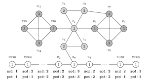
Example 3.1: Consider the graph $G$ in Figure 3. The subgraph induced by $\{v_{6},v_{7},\cdots,v_{13}\}$ is the $3$-core of $G$ because in the induced graph, every vertex has a degree at least $3$. There does not exist a $4$-core in $G$. We have ${\mathsf{core}}(v_{i})=3$ for $6\leq i\leq 13$, ${\mathsf{core}}(v_{i})=2$ for $1\leq i\leq 5$ and ${\mathsf{core}}(u_{i})=1$ for $0\leq i\leq 2000$. Also, $\{v_{1},v_{2},v_{3},v_{4},v_{5}\}$ and $\{u_{i}\}$ are the unique $2$-subcore and $1$-subcore of $G$, respectively. There are two $3$-subcores in $G$ by $\{v_{6},v_{7},v_{8},v_{9}\}$ and $\{v_{10},v_{11},v_{12},v_{13}\}$.

Core Decomposition: Given a graph $G$, the problem of computing the core number for each $u\in V(G)$ is called core decomposition. [4] proposed an $\mathcal{O}(m+n)$ algorithm, denoted as $\mathsf{CoreDecomp}$, whose sketch is shown in Algorithm 1. The general idea is as follows: To compute the $k$-core $G_{k}$ of $G$, it repeatedly remove those vertices (and their adjacent edges) whose degrees are less than $k$. When there is no more vertex to remove, the resulting graph is the $k$-core of $G$.

Core Maintenance: The problem of core maintenance is to maintain the $k$-core by maintaining the core numbers, when edges are inserted to or removed from $G$. This is because it is known that $k$-core $G_{k}$ can be efficiently computed using the core numbers of the vertices, since a vertex $u\in V(G_{k})$ if and only if ${\mathsf{core}}(u)\geq k$. In addition, an index can be constructed for core numbers of the vertices. From now on, we use the notation $V^{*}$ to denote the set of vertices whose core numbers need to be updated after inserting or removing an edge. The insertion or removal of vertices can be simulated as a sequence of edge insertions and removals. Hence in this paper, we focus on efficient core maintenance under edge updates.

1 $k\leftarrow 1$;

2 while $G$ is not empty do

3       while $\exists u\in V(G)$ such that ${\mathsf{deg}}(u)<k$ do

4             let $u$ be a vertex with ${\mathsf{deg}}(u)<k$;

5             ${\mathsf{deg}}(w)\leftarrow{\mathsf{deg}}(w)-1$ for each $w\in{\mathsf{nbr}}(u)$;

6             remove $u$ and its adjacent edges from $G$;

7             ${\mathsf{core}}(u)\leftarrow k-1$;

8            

9      $k\leftarrow k+1$;

10      

11return $\mathsf{core}$ ;

Algorithm 1 $\mathsf{CoreDecomp}$ ($G$)

Here we present two theorems given in [11, 13] based on which the correctness of our algorithms is proved.

Theorem 3.1: [11, 13] After inserting to (resp. removing from) $G=(V,E)$ an edge, the core number of a vertex $u\in V$ increases (resp. decreases) by at most $1$.

Theorem 3.2: [11, 13] Suppose an edge $(u,v)$ with $K={\mathsf{core}}(u)\leq{\mathsf{core}}(v)$ is inserted to (resp. removed from) $G$. Suppose $V^{*}$ is non-empty. We have the following: (1) if ${\mathsf{core}}(u)<{\mathsf{core}}(v)$, then $u\in V^{*}$ and $V^{*}\subseteq{\mathsf{sc}}(u)$; (2) if ${\mathsf{core}}(u)={\mathsf{core}}(v)$, then both $u$ and $v$ are in $V^{*}$ (resp. at least one of $u$ and $v$ is in $V^{*}$) and $V^{*}\subseteq{\mathsf{sc}}(u)\cup{\mathsf{sc}}(v)$; (3) the induced subgraph of $V^{*}$ in $G\cup\{(u,v)\}$ (resp. $G$) is connected.

Theorem 1 suggests that we only need to find $V^{*}$, the set of vertices whose core numbers need to be updated. Once $V^{*}$ is found, we can then increase (or decrease) ${\mathsf{core}}$ for vertices in $V^{*}$ by $1$ accordingly. Theorem 1 suggests two things. (1) Only vertices $w$ with ${\mathsf{core}}(w)=K$ may be in $V^{*}$, i.e., ${\mathsf{core}}(w)$ may need to be updated. (2) We can search for $V^{*}$ in a small local region near the inserted (or removed) edge (i.e., the subcores containing $u$ and $v$), rather than in the whole $G$.

IV The Traversal Algorithm

In this section, we discuss the state-of-the-art core maintenance solution, called the traversal algorithm [13], which is designed on top of two important notions, namely ${\mathsf{mcd}}(u)$ and ${\mathsf{pcd}}(u)$. We introduce them below.

The max-core degree of a vertex $u$, denoted as ${\mathsf{mcd}}(u)$, is defined as the number of $u$’s neighbors, $w$, such that ${\mathsf{core}}(w)\geq{\mathsf{core}}(u)$. Intuitively, ${\mathsf{mcd}}(u)$ counts $u$’s neighbors in the $({\mathsf{core}}(u))$-core. By the definition of $k$-core, ${\mathsf{mcd}}(u)\geq{\mathsf{core}}(u)$. The pure-core degree of a vertex $u$, denoted as ${\mathsf{pcd}}(u)$, is defined as the number of $u$’s neighbors, $w$, such that either ${\mathsf{core}}(w)={\mathsf{core}}(u)$ and ${\mathsf{mcd}}(w)>{\mathsf{core}}(w)$ or ${\mathsf{core}}(w)>{\mathsf{core}}(u)$. The main difference between ${\mathsf{pcd}}$ and ${\mathsf{mcd}}$ is that ${\mathsf{pcd}}(u)$ further excludes neighbors $w$ with ${\mathsf{core}}(w)={\mathsf{core}}(u)$ and ${\mathsf{mcd}}(w)={\mathsf{core}}(w)$. Thus ${\mathsf{pcd}}(u)\leq{\mathsf{mcd}}(u)$. We show ${\mathsf{mcd}}(u_{i})$ and ${\mathsf{pcd}}(u_{i})$, for $\{u_{i}\}$, in Figure 3 and an example below which demonstrates why ${\mathsf{mcd}}$ and ${\mathsf{pcd}}$ are useful.

Example 4.1: Suppose edge $(v_{4},u_{0})$ is inserted to $G$ in Figure 3. Due to the newly inserted edge, both ${\mathsf{mcd}}(u_{0})$ and ${\mathsf{pcd}}(u_{0})$ become $4$. By Theorem 1, only core numbers of vertices in $\{u_{i}\}$ may need to be updated. We show two cases. First, consider $u_{1999}$. $u_{1999}$ can not be in the $2$-core of $G\cup\{(v_{4},u_{0})\}$, because the number of its neighbors in the new $2$-core is upper bounded by ${\mathsf{mcd}}(u_{1999})<2$. To see why ${\mathsf{mcd}}(u_{1999})$ is an upper bound, recall that by Theorem 1 and Theorem 1, only vertices with core numbers greater than or equal to $1$ may be in the new $2$-core. Second, consider $u_{1997}$. Regarding ${\mathsf{mcd}}(u_{1997})$, the max possible number of $u_{1997}$’s neighbors in the new $2$-core is ${\mathsf{mcd}}(u_{1997})=2$, so ${\mathsf{core}}(u_{1997})$ may need to be updated. Regarding ${\mathsf{pcd}}(u_{1997})$, the max possible number of $u_{1997}$’s neighbors in the new $2$-core is ${\mathsf{pcd}}(u_{1997})=1<2$. ${\mathsf{pcd}}(u_{1997})$ does not count $u_{1999}$, which can not be in the new $2$-core because ${\mathsf{mcd}}(u_{1999})={\mathsf{core}}(u_{1999})=1$. Hence, with ${\mathsf{pcd}}(u_{1997})$, there is no need to update ${\mathsf{core}}(u_{1997})$.

IV-A The Traversal Insertion Algorithm

The insertion algorithm employs an expand-shrink framework to determine $V^{*}$, the set of vertices whose core numbers need to be updated. It works as follows: When a new edge $(u,v)$ with $K={\mathsf{core}}(u)\leq{\mathsf{core}}(v)$ is inserted into $G$, it first updates ${\mathsf{mcd}}$ and ${\mathsf{pcd}}$ accordingly based on the old ${\mathsf{core}}$ values. Because ${\mathsf{core}}(u)\leq{\mathsf{core}}(v)$, it selects $u$ as the root. Based on Theorem 1 and the discussion above, in order to find $V^{*}$, it issues a DFS starting from the root and only visits $w$ with ${\mathsf{core}}(w)=K$ and ${\mathsf{mcd}}(w)>K$. The algorithm maintains a value ${\mathsf{cd}}(w)$ for every vertex $w$ visited, where ${\mathsf{cd}}(w)$ represents the max possible number of $w$’s neighbors in the new $(K+1)$-core. Initially ${\mathsf{cd}}(w)={\mathsf{pcd}}(w)$. During the DFS, it stops the search when the vertex $w$ visited is confirmed to be $w\notin V^{*}$ (i.e., ${\mathsf{cd}}(w)\leq K$). It evicts $w$ (i.e., mark $w\notin V^{*}$) and decreases the ${\mathsf{cd}}$ values of its neighbors by $1$. In addition, it conducts a backward search from $w$ to find more visited vertices to evict. Such a process is called an eviction propagation. After the eviction propagation ends, it will continue DFS in the original order, skipping $w$. When the algorithm terminates, it is guaranteed that all visited but not evicted vertices constitute $V^{*}$. As the final step, it needs to update ${\mathsf{mcd}}$ and ${\mathsf{pcd}}$ for later insertions and removals.

Example 4.2: Suppose $(v_{4},u_{0})$ is inserted to the graph $G$ in Figure 3. The initial ${\mathsf{cd}}$ values for all $u_{i}$ are shown in Figure 4. The traversal insertion algorithm selects $u_{0}$ as the root and issues a DFS from $u_{0}$. The DFS recursively visits those vertices $u_{i}$ with ${\mathsf{core}}(u_{i})=1$ and ${\mathsf{mcd}}(u_{i})>1$. Without loss of generality, assume the DFS first traverses the right part of $u_{0}$. When DFS reaches $u_{1997}$, it finds ${\mathsf{cd}}(u_{1997})\leq 1$, thus ${\mathsf{core}}(u_{1997})$ does not need to be updated and $u_{1997}$ is evicted. Further, the eviction propagates back to $u_{1}$ as follows: Due to eviction of $u_{1997}$, ${\mathsf{cd}}(u_{1995})$ is decreased by $1$ and becomes $1$. Thus $u_{1995}$ is also evicted. This process continues and finally it evicts all $u_{1997}$, $\cdots$, $u_{1}$. The DFS then traverses the left part. Similarly, $u_{2}$, $\cdots$, $u_{1998}$ are all evicted. At last, $u_{0}$ is the only vertex that is visited but not evicted and therefore $V^{*}=\{u_{0}\}$.

Figure 4: Illustration of Example IV-A

In Example IV-A, although $u_{0}$ is the only vertex whose core number needs to be updated, the traversal insertion algorithm needs to visit much more (specifically, 1,999) vertices to determine $V^{*}=\{u_{0}\}$. As shown in Figure 1 and Figure 2, such an issue is not rare and hurts the performance significantly.

Such a high overhead is due to the potential large search space used by the algorithm. Let $V^{\prime}$ be the search space, i.e., the set of vertices that the traversal insertion algorithm visits, in order to obtain $V^{*}$. In order to show an upper bound of $|V^{\prime}|$, we introduce a concept called pure-core [13], in Definition 4.

Definition 4.1: For each $u\in V(G)$, its pure-core, denoted as ${\mathsf{pc}}(u)$, is defined as ${\mathsf{pc}}(u)=\{u\}\cup\mathcal{PC}$, where $\mathcal{PC}$ is a set of vertices that satisfies the following 3 conditions: (1) for $\forall w\in\mathcal{PC}$, ${\mathsf{mcd}}(w)>{\mathsf{core}}(w)$ and ${\mathsf{core}}(w)={\mathsf{core}}(u)$; (2) $G(\{u\}\cup\mathcal{PC})$ is connected; and (3) $\mathcal{PC}$ is maximal.

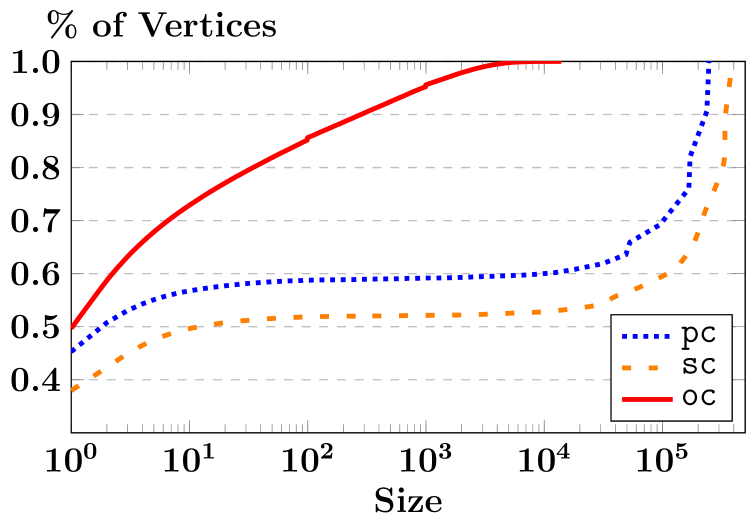
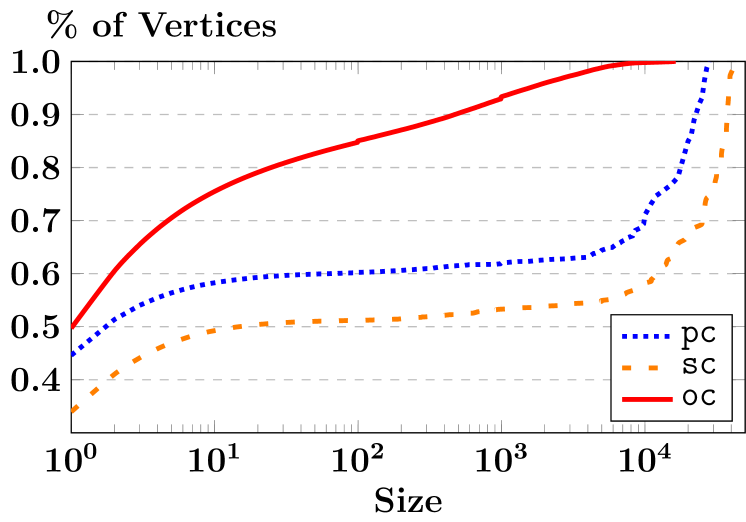
It is not hard to observe that $V^{\prime}\subseteq{\mathsf{pc}}(u)\cup{\mathsf{pc}}(v)$ when an edge $(u,v)$ is inserted; that is, the size of pure-cores decides the max number of vertices that are visited by the traversal insertion algorithm. We show the cumulative distribution of ${\mathsf{pc}}$, for two of the largest graphs tested (Table I), namely, $\mathsf{Patents}$ and $\mathsf{Orkut}$, in Figure 5. Figure 5 shows the % of vertices whose pure-cores (${\mathsf{pc}}$) are smaller than a certain size $s$ for all possible $s$ in the x-axis. We observe that ${\mathsf{pc}}$ is with high variance in distribution. Moreover, many vertices have a very large pure-core size. For example, for both graphs, more than 10% of vertices have their pure-core size greater than 10,000, which is very high and leads to high overhead.

(a) $\mathsf{Patents}$

(b) $\mathsf{Orkut}$

Figure 5: Cumulative size distribution of ${\mathsf{pc}}$, ${\mathsf{sc}}$, and ${\mathsf{oc}}$.

IV-B The Traversal Removal Algorithm

The removal algorithm first updates ${\mathsf{mcd}}$ and ${\mathsf{pcd}}$ when an edge $(u,v)$ with $K={\mathsf{core}}(u)\leq{\mathsf{core}}(v)$ is removed from $G$. The algorithm uses the similar idea as shown in the $\mathsf{CoreDecomp}$ algorithm (Algorithm 1) to find $V^{*}$. It works as follows. Let $u$ be the root (if ${\mathsf{core}}(v)=K$, $v$ should also be a root). Starting from the root(s), the algorithm finds $V^{*}$ by repeatedly removing vertices $w$ with ${\mathsf{core}}(w)=K$ and ${\mathsf{cd}}(w)<K$ and appending $w$ to $V^{*}$, where ${\mathsf{cd}}(w)$ is initialized as ${\mathsf{mcd}}(w)$ and counts the max possible # of neighbors of $w$ in the new $K$-core. When $w$ is removed, the algorithm decreases ${\mathsf{core}}(w)$ by 1. Since ${\mathsf{core}}(w)$ becomes $K-1$, for $z\in{\mathsf{nbr}}(w)$ with ${\mathsf{core}}(z)=K$, ${\mathsf{cd}}(z)$ is decreased by $1$. Accordingly, if ${\mathsf{cd}}(z)$ becomes smaller than $K$, $z$ is also removed. Such a process continues until no more vertex can be removed and requires only $\mathcal{O}(\sum_{v\in V^{*}}{\mathsf{deg}}(v))$ time. At last, ${\mathsf{mcd}}$ and ${\mathsf{pcd}}$ need to be updated for later insertions and removals.

It is important to note that ${\mathsf{pcd}}$ needs to be maintained for the following possible edge insertions, even though ${\mathsf{pcd}}$ is not required in the traversal removal algorithm. The performance of the algorithm is completely dominated by the maintenance of $\mathsf{pcd}$. By the definition, ${\mathsf{pcd}}(u)$ may be affected by a vertex $w$ that is $2$ hops away from $u$. If ${\mathsf{core}}(u)$ is decreased by $1$ for every $u\in V^{*}$, in the worst case, $\mathcal{O}(\sum_{v\in{\mathsf{nbr}}(V^{*})}{\mathsf{deg}}(v))$ vertices may have their ${\mathsf{pcd}}$ affected.

Both the traversal insertion algorithm and the traversal removal algorithm suffer from the same performance problem to maintain $\mathsf{pcd}$, and the cost to maintain ${\mathsf{pcd}}$ is high. In some cases, although the algorithm visits only a small number of vertices to find $V^{*}$, the benefit brought however is neutralized by the cost to maintain $\mathsf{pcd}$.

V An Order-Based Algorithm

There are two main issues in the traversal algorithm. One is the cost of finding $V^{*}$ and the other is the cost of maintaining $\mathsf{pcd}$. The issue of finding $V^{*}$ by the traversal insertion algorithm is more serious than the traversal removal algorithm. Unlike the traversal removal algorithm, the traversal insertion algorithm does not take the idea shown in $\mathsf{CoreDecomp}$ (Algorithm 1). Recall the idea shown in $\mathsf{CoreDecomp}$. When a new edge $(u,v)$ with $K={\mathsf{core}}(u)\leq{\mathsf{core}}(v)$ is inserted, it identifies $V^{*}$ by repeatedly removing vertices whose degrees are less than $K+1$. Then, $V^{*}$ is identified as the set of the vertices taken from the vertices remained if their original core numbers are $K$. The main reason that the traversal insertion algorithm does not do so is due to the fact that the cost of core maintenance otherwise will become as high as the cost of core decomposition.

In this work, we revisit the idea presented in $\mathsf{CoreDecomp}$ (Algorithm 1), and design new algorithms to significantly improve the performance for core maintenance for both edge insertions and removals. The challenges by taking the idea behind $\mathsf{CoreDecomp}$ for core maintenance are twofold. First, we need to find an efficient way to maintain the degrees of the neighbors when a vertex is removed during core maintenance, instead of removing vertices as done by $\mathsf{CoreDecomp}$. In other words, we need to maintain the order used by $\mathsf{CoreDecomp}$, but we cannot afford to compute the order in core maintenance. Second, because the number of vertices to be affected can be large, it is impractical to remove vertices online one-by-one. The solution we propose to address the challenges is to introduce an order, called $k$-order, with which we can reduce the core maintenance cost.

Consider a graph $G$. Let $G^{0}=G$ and $G^{i}$ be the graph after $i$ insertion/removal of edges. The $k$-order is initially defined over $G^{0}$, which is the order by $\mathsf{CoreDecomp}$ (Algorithm 1). In details, the $k$-order, denoted as $\preceq$, is that $u\preceq v$ if and only if vertex $u$ will be removed in Algorithm 1 before $v$. It is obvious that $u\preceq v$ if ${\mathsf{core}}(u)<{\mathsf{core}}(v)$. It is worth mentioning that either $u\preceq v$ or $v\preceq u$ is possible when ${\mathsf{core}}(v)={\mathsf{core}}(u)$. In such a case, one of the two can be used, if it can be obtained by Algorithm 1. When $\preceq$ is determined for $G^{0}$, we will maintain the order $\preceq$ such that it is a $k$-order for graph $G^{i}$ for $i>0$. In the following, for simplicity, we use $G$ instead of $G^{i}$ and $G^{\prime}$ instead of $G^{i+1}$ when the context is clear.

Definition 5.1: ($k$-order) Given a graph $G$, let $G^{0}$ be $G$. Assume $G^{i}$ is a graph after $i$ insertion/removal of edges. The $k$-order $\preceq$ is defined for any $u$ and $v$ over $G^{i}$ as follows.

• When ${\mathsf{core}}(u)<{\mathsf{core}}(v)$, $u\preceq v$.

• When ${\mathsf{core}}(u)={\mathsf{core}}(v)$, $u\preceq v$ if $u$ is removed before $v$ by $\mathsf{CoreDecomp}$ (Algorithm 1) for $G^{i}$.

A $k$-order, $(v_{1},v_{2},\ldots,v_{n})$, for $v_{i}\in V(G)$, is an instance of all the possible vertex sequences produced by Algorithm 1. The transitivity holds; that is, $u\preceq v$ if $u\preceq w$ and $w\preceq v$.

Definition 5.2: (remaining degree) For a vertex $u$ in $G^{i}$, the remaining degree of $u$, denoted as ${\mathsf{deg}}^{+}(u)$, is defined as: ${\mathsf{deg}}^{+}(u)=|\{v\in{\mathsf{nbr}}(u):u\preceq v\}|$.

Here, ${\mathsf{deg}}^{+}(u)$ is the degree of the neighbors that appear after $u$. Given $k$-order $\preceq$ defined, we use $O_{k}$ to denote the sequence of vertices in $k$-order whose core numbers are $k$. It is obvious that for a vertex $u$ in $O_{k}$, ${\mathsf{deg}}^{+}(u)\leq k$. And we have a sequence of $O_{0}O_{1}O_{2}\cdots$, where $O_{i}\preceq O_{j}$ if $i<j$. It is clear that $\preceq$ defined over the sequence of $O_{0}O_{1}O_{2}\cdots$ is implied by the $k$-order ($\preceq$).

Lemma 5.1: Given a graph $G$, the order ($\preceq$) on $O_{0}O_{1}O_{2}\cdots$ over $V(G)$ is the $k$-order if and only if ${\mathsf{deg}}^{+}(v)\leq k$ for every vertex $v$ in $O_{k}$, for $\forall k$.

Proof: Please refer to the appendix.

By Lemma V, in order to maintain the $k$-order, we maintain every $O_{k}$ such that $\forall v\in O_{k}$, ${\mathsf{deg}}^{+}(v)\leq k$.

Figure 6: The $k$-order for $G$ in Figure 3

Example 5.1: In Figure 6, we show a $k$-order for the graph $G$ (Figure 3) by showing $O_{1}$, $O_{2}$, $O_{3}$. In $O_{1}$, $u_{i}\preceq u_{j}$ if $i>j$. In $O_{2}$, $v_{4}\preceq v_{5}\preceq v_{3}\preceq v_{2}\preceq v_{1}$. In $O_{3}$, $v_{8}\preceq v_{9}\preceq v_{7}\preceq v_{6}\preceq v_{13}\preceq v_{12}\preceq v_{11}\preceq v_{10}$. The $k$-order is one of the orders computed by Algorithm 1 for the graph $G$. Consider the vertex $v_{2}$ in $G$. $v_{2}$ has three neighbors: $v_{1}$, $v_{3}$, and $v_{7}$. Here, both $v_{1}$ and $v_{3}$ are in $O_{2}$ and $v_{7}$ is in $O_{3}$, because ${\mathsf{core}}(v_{1})={\mathsf{core}}(v_{3})=2$ and ${\mathsf{core}}(v_{7})=3$. In terms of $k$-order, $v_{3}\preceq v_{2}\preceq v_{1}\preceq v_{7}$. Therefore, ${\mathsf{deg}}^{+}(v_{2})=2$. The ${\mathsf{deg}}^{+}(v_{i})$ for $v_{i}$ is shown as a number next to $v_{i}$ in Figure 6.

(a) Identification of $V^{*}$ in the Insertion Algorithm

(b) Maintenance of $k$-Orders

Figure 7: Algorithm Framework

V-A An Algorithm Overview

We design new algorithms to deal with an edge $(u,v)$ to be inserted into or removed from $G$. For simplicity, we assume $K={\mathsf{core}}(u)\leq{\mathsf{core}}(v)$, and $u\preceq v$. Here, $u\in O_{K}$. Let the resulting graph of the insertion/removal be $G^{\prime}$. There are two key issues in our algorithms. First, we need to identify $V^{*}$, the set of vertices whose core numbers need to be updated, efficiently using the $k$-order $\preceq$ of $G$. Second, we need to maintain the $k$-order efficiently such that the new order $\preceq^{\prime}$ is the $k$-order of $G^{\prime}$.

Edge Insertion: Suppose an edge $(u,v)$ is inserted for $u\in O_{K}$ and $u\preceq v$. $V^{*}$ can be computed efficiently. We show the main ideas below.

1. A vertex $w$ cannot be in $V^{*}$ if $w\in O_{L}$ for $L<K$.

2. A vertex $w$ cannot be in $V^{*}$ if $w\in O_{L}$ for $K<L$.

3. A vertex $w$ in $O_{K}$ cannot be in $V^{*}$ if $w\preceq u$.

4. A vertex $w$ in $O_{K}$ may be in $V^{*}$ if $u\preceq w$ and there is a path $w_{0},w_{1},w_{2},\cdots,w_{t}$ such that $w_{0}=u$, $w_{t}=w$, $(w_{i},w_{i+1})\in E$ and $w_{i}\preceq w_{i+1}$ for $0\leq i<t$.

5. A vertex $w$ that satisfies (i4) is not necessarily in $V^{*}$.

Items (i1) and (i2) are proved by Theorem 1. We further explain other points using Figure 7(a). In $O_{K}$, a vertex $w$ can not be in $V^{*}$ if $w\preceq u$ by (i3). Figure 7(a) also shows that the vertices reachable from $u$ by (i4) are possibly in $V^{*}$, but not all the vertices reachable from $u$ are included in $V^{*}$ by (i5).

To compute $V^{*}$, we design an efficient algorithm that can “jump” from a candidate of $V^{*}$ to another following the $k$-order of $G$. Therefore, the search space for obtaining $V^{*}$ is significantly reduced. Suppose $V^{*}$ is obtained. To obtain the $k$-order $\preceq^{\prime}$ of the resulting graph $G^{\prime}$, as shown in Figure 7(b), the set of vertices in $V^{*}$ in $O_{K}$ will be moved to the beginning of $O_{K+1}$. The $k$-order by the insertion of $(u,v)$ remains unchanged for all vertices in $O_{L}$, for either $K<L$ or $K>L$, in $G^{\prime}$. The $k$-order for the vertices that will be in the same $O_{K}$ in the resulting graph $G^{\prime}$ needs small adjustment. It is guaranteed that only vertices visited by our algorithm may have their positions changed. The new order $\preceq^{\prime}$ is a valid $k$-order of $G^{\prime}$.

Edge Removal: Suppose an edge $(u,v)$ is removed. We adopt the similar idea presented in the traversal removal algorithm to find $V^{*}$. However, we maintain the $k$-order instead of ${\mathsf{pcd}}$ used in the traversal removal algorithm to achieve high efficiency. To obtain the $k$-order of $G^{\prime}$, we move the vertices in $V^{*}$ from $O_{K}$ to the end of $O_{K-1}$, without affecting the original vertices in $O_{K-1}$, as shown in Figure 7(b). The resulting order is guaranteed to be a valid $k$-order of $G^{\prime}$. We present more details when we discuss our removal algorithm.

V-B The Order-Insertion Algorithm

Identifying $V^{*}$: Suppose an edge $(u,v)$ is inserted for $u\in O_{K}$ and $u\preceq v$. Since (i1) and (i2) are trivial, we focus on (i3) – (i5). We call the vertex $u$ as a root since $u\preceq v$. Note that by insertion of $(u,v)$, ${\mathsf{deg}}^{+}(u)$ is increased by $1$ to reflect the insertion of $(u,v)$, while ${\mathsf{deg}}^{+}(v)$ remains unchanged. Next, we show in Lemma V-B that no vertices in $O_{K}$ can be in $V^{*}$ if $u$ does not have sufficient neighbors that appear after $u$ in $k$-order, i.e., ${\mathsf{deg}}^{+}(u)\leq K$. This implies that we need to update core numbers of vertices in $O_{K}$ only if ${\mathsf{deg}}^{+}(u)>K$. We also show in Lemma V-B that there is no need to update the vertices that appear before $u$ in $O_{K}$, when ${\mathsf{deg}}^{+}(u)>K$. For the vertices that appear after $u$ in $k$-order in $O_{K}$, we show the cases we need to consider.

Lemma 5.2: No core number needs to be updated for vertices in $O_{K}$, if ${\mathsf{deg}}^{+}(u)\leq K$ after increasing ${\mathsf{deg}}^{+}(u)$ by $1$.

Lemma 5.3: No vertex $w$ that appears before $u$ in $O_{K}$ can be in $V^{*}$, if ${\mathsf{deg}}^{+}(u)>K$ after increasing ${\mathsf{deg}}^{+}(u)$ by $1$.

Proof: The proof of Lemma V-B and V-B is in the appendix.

Example 5.2: Reconsider Example IV-A. Suppose edge $(v_{4},u_{0})$ is inserted to $G$, where $u_{0}\preceq v_{4}$ in $G$. Then, ${\mathsf{deg}}^{+}(u_{0})$ becomes $2$. Note that $u_{0}$ is in $O_{1}$ before the new edge is inserted. By Lemma V-B, all vertices that occur before $u_{0}$ in $O_{1}$ (the rectangle in Figure 6) can not be in $V^{*}$. Reconsider $u_{0}$, ${\mathsf{deg}}^{+}(u_{0})=2$ implies that $u_{0}$ has at least two neighbors appearing after $u_{0}$ in the $k$-order, which are $v_{4}$ and $v_{5}$ in this example. Hence, $u_{0}$ will be in the $2$-core of the new graph $G\cup\{(v_{4},u_{0})\}$. We have $V^{*}=\{u_{0}\}$. As shown in this example, our approach achieves high efficiency, because we only need to visit $1$ vertex (i.e., $u_{0}$), while the traversal insertion algorithm needs to visit $1,999$ vertices in total to identify $V^{*}$.

In Example V-B, vertex $u_{0}$ is the last vertex in $O_{1}$. Generally, when a new edge $(u,v)$ is inserted for $u\in O_{K}$ and $u\preceq v$, $u$ can be in any position in $O_{K}$. There may be vertices appearing after $u$ in $O_{K}$. Among all such vertices, we further discuss whether a vertex $w$ with $u\preceq w$ in $O_{K}$ can be a potential candidate in $V^{*}$. We first introduce the concept of candidate degree.

Definition 5.3: (candidate degree) For a vertex $w$ in $O_{K}$, the candidate degree of $w$, denoted as ${\mathsf{deg}}^{*}(w)$, is defined as: ${\mathsf{deg}}^{*}(w)$ $=|\{w^{\prime}\in{\mathsf{nbr}}(w):w^{\prime}\preceq w\land{\mathsf{core}}(w^{\prime})=K\land w^{\prime}\textnormal{ is a potential candidate of $V^{*}$}\}|$.

In order to test whether a vertex $w$ can be a potential candidate in $V^{*}$, we use ${\mathsf{deg}}^{*}(w)+{\mathsf{deg}}^{+}(w)$. Recall that ${\mathsf{deg}}^{+}(w)$ (Definition V) counts the number of $w$’s neighbors after $w$ in the $k$-order, whose core numbers are greater than or equal to $K$. In other words, ${\mathsf{deg}}^{+}(w)$ counts how many $w$’s neighbors after $w$ can be in the new $(K+1)$-core. Therefore, ${\mathsf{deg}}^{+}(w)+{\mathsf{deg}}^{*}(w)$ upper bounds the number of $w$’s neighbors in the new $(K+1)$-core. Specifically, if ${\mathsf{deg}}^{+}(w)+{\mathsf{deg}}^{*}(w)\leq K$, $w$ does not have sufficient neighbors in the new $(K+1)$-core, thus $w$ cannot be in $V^{*}$; if ${\mathsf{deg}}^{+}(w)+{\mathsf{deg}}^{*}(w)>K$ otherwise, $w$ is a potential candidate.

Initially, ${\mathsf{deg}}^{*}(w)=0$ for each $w\in O_{K}$ since we have not found any candidate yet. We start from $u$ and visit vertices in $O_{K}$ following the $k$-order. For each vertex $w$ being visited, we discuss two cases.

Case-1 (${\mathsf{deg}}^{*}(w)+{\mathsf{deg}}^{+}(w)>K$): Since $w$ potentially has more than $K$ neighbors in the new $(K+1)$-core, $w$ may be in $V^{*}$, i.e., ${\mathsf{core}}(w)$ may become $K+1$. We put $w$ in a set $V_{C}$, which records all current visited potential candidates. Further, each neighbor $w^{\prime}$ of $w$ that $w\preceq w^{\prime}$ in $O_{K}$, obtains one candidate degree (${\mathsf{deg}}^{*}(w^{\prime})$ increased by $1$) to reflect the existence of $w$. In other words, for each such $w^{\prime}$, the potential number of neighbors in the new $(K+1)$-core increases by $1$. Note that $u$ is a special example in this case because ${\mathsf{deg}}^{*}(u)=0$ and ${\mathsf{deg}}^{+}(u)>K$. We next visit the vertex that is next to $w$ in the $k$-order.

Case-2 (${\mathsf{deg}}^{*}(w)+{\mathsf{deg}}^{+}(w)\leq K$): $w$ does not have sufficient neighbors in the new $(K+1)$-core, since ${\mathsf{deg}}^{*}(w)+{\mathsf{deg}}^{+}(w)\leq K$. Therefore, $w\notin V^{*}$. There are two subcases, namely, Case-2a for ${\mathsf{deg}}^{*}(w)=0$ and Case-2b for ${\mathsf{deg}}^{*}(w)\neq 0$.

For Case-2a, $w$ cannot be in $V^{*}$. We next visit the vertex $w^{\prime\prime}$ which is next to $w$ in the $k$-order. It is possible that $w^{\prime\prime}$ again is in Case-2a, implying that $w^{\prime\prime}\notin V^{*}$. More generally, let $w^{\prime}$ be the first vertex after $w$ in $O_{K}$ such that ${\mathsf{deg}}^{*}(w^{\prime})\neq 0$. For any $w^{\prime\prime}$ in the range $[w,w^{\prime})$ in the $k$-order, ${\mathsf{deg}}^{*}(w^{\prime\prime})=0$. As a result, these $w^{\prime\prime}$s cannot be in $V^{*}$ and we can skip them, directly “jump” to visit $w^{\prime}$ next. Specially, if such $w^{\prime}$ does not exist, all vertices after $w$ cannot be in $V^{*}$.

For Case-2b, it differs from Case-2a for ${\mathsf{deg}}^{*}(w)\neq 0$. Here, ${\mathsf{deg}}^{*}(w)\neq 0$ implies that some neighbor $w^{\prime}$ that $w^{\prime}\preceq w$ is considered as a potential candidate. In other words, ${\mathsf{deg}}^{*}(w^{\prime})+{\mathsf{deg}}^{+}(w^{\prime})>K$ (refer to Case-1 where $w^{\prime}$ is in the position of $w$ in Case-1). Excluding $w$ from $V^{*}$ results in ${\mathsf{deg}}^{+}(w^{\prime})$ to be decreased by $1$ for each neighbor vertex $w^{\prime}$ that $w^{\prime}\preceq w$ and $w^{\prime}\in V_{C}$. Recall that $V_{C}$ is the set of vertices that currently are candidates for $V^{*}$. If ${\mathsf{deg}}^{*}(w^{\prime})+{\mathsf{deg}}^{+}(w^{\prime})\leq K$ after such a update, then we can remove $w^{\prime}$ from $V_{C}$ since $w^{\prime}$ is not a candidate any more, which may further result in other potential candidates to be removed from $V_{C}$. The situation can be demonstrated using Figure 8. Suppose $w^{\prime}$ is not a potential candidate after ${\mathsf{deg}}^{+}(w^{\prime})$ decreases by 1. Then (1) ${\mathsf{deg}}^{+}(w^{\prime\prime}_{1})$ is decreased by $1$ for each neighbor $w^{\prime\prime}_{1}$ of $w^{\prime}$ that $w^{\prime\prime}_{1}\in V_{C}$ and $w^{\prime\prime}_{1}\preceq w^{\prime}$; (2) ${\mathsf{deg}}^{*}(w^{\prime\prime}_{2})$ is decreased by $1$ for each neighbor $w^{\prime\prime}_{2}$ of $w^{\prime}$ that $w^{\prime\prime}_{2}\in V_{C}$ and $w^{\prime}\preceq w^{\prime\prime}_{2}\preceq w$; (3) ${\mathsf{deg}}^{*}(w^{\prime\prime}_{3})$ is decreased by $1$ for each neighbor $w^{\prime\prime}_{3}$ of $w^{\prime}$ that $w\preceq w^{\prime\prime}_{3}$. For $w^{\prime\prime}_{1}$ and $w^{\prime\prime}_{2}$, they may not be a candidate any more after update and will be removed from $V_{C}$. The chain effect can further propagate. For $w^{\prime\prime}_{3}$, we just update its ${\mathsf{deg}}^{*}$ and it will be processed when we visit it later. Recall that we visit vertices in $O_{K}$ following the $k$-order. We choose the vertex next to $w$ in the $k$-order as the next vertex to visit.

When we reach the end of $O_{K}$, $V^{*}=V_{C}$. We explain the rationale as follows. For each $w\in V_{C}$, we have (1) ${\mathsf{deg}}^{*}(w)=|\{w^{\prime}\in{\mathsf{nbr}}(w):w^{\prime}\in V_{C}\land w^{\prime}\preceq w\}|$, and (2) ${\mathsf{deg}}^{+}(w)=|\{w^{\prime}\in{\mathsf{nbr}}(w):w^{\prime}\in V_{C}\land w\preceq w^{\prime}\textnormal{ or }{\mathsf{core}}(w^{\prime})>K\}|$. Therefore, ${\mathsf{deg}}^{*}(w)+{\mathsf{deg}}^{+}(w)$ is the number of the neighbors of $w$ that are in $V_{>K}\cup V_{C}$ and is greater than or equal to $K+1$, where $V_{>K}=\{v\in V:{\mathsf{core}}(v)>K\}$. Hence, $G(V_{>K}\cup V_{C})$ is the new $(K+1)$-core of $G^{\prime}$. In other words, $V^{*}=V_{C}$.

Figure 8: Demonstration of Case-2b.

Maintaining $k$-order: Since the core numbers of vertices in $V^{*}$ change from $K$ to $K+1$, we need to obtain two new sequences $O^{\prime}_{K}$ and $O^{\prime}_{K+1}$ for vertices with core number $K$ and $K+1$ respectively, such that the new order $\preceq^{\prime}$ over $O_{0}\cdots O_{K-1}O^{\prime}_{K}O^{\prime}_{K+1}O_{K+2}\cdots$ is a $k$-order of $G^{\prime}$. By Lemma V, we only need to guarantee that (1) ${\mathsf{deg}}^{+}(w)\leq K$ for $\forall w\in O^{\prime}_{K}$ and (2) ${\mathsf{deg}}^{+}(w)\leq K+1$ for $\forall w\in O^{\prime}_{K+1}$. We discuss $O^{\prime}_{K}$ first.

In order to construct $O^{\prime}_{K}$, the main idea is to append a vertex $w$ to $O^{\prime}_{K}$ when we encounter a vertex $w$ with ${\mathsf{deg}}^{*}(w)+{\mathsf{deg}}^{+}(w)\leq K$ during the process of identifying $V^{*}$. The rationale is that ${\mathsf{deg}}^{*}(w)+{\mathsf{deg}}^{+}(w)$ is exactly the number of $w$’s neighbors that have not been appended to $O^{\prime}_{K}$ yet or that have core number greater than $K$. Therefore, ${\mathsf{deg}}^{*}(w)+{\mathsf{deg}}^{+}(w)$ is the number of $w$’s neighbors that will appear after $w$ in the new $k$-order. The new ${\mathsf{deg}}^{+}(w)$ is set as ${\mathsf{deg}}^{*}(w)+{\mathsf{deg}}^{+}(w)$. We give the details. Let $w$ be the vertex currently being visited.

• Case-1: $w$ cannot be appended to $O^{\prime}_{K}$ temporarily and thus is skipped.

• Case-2a: $w$ is appended to $O^{\prime}_{K}$. Because ${\mathsf{deg}}^{*}(w)=0$, ${\mathsf{deg}}^{+}(w)$ remains unchanged.

• Case-2b: $w$ is appended to $O^{\prime}_{K}$ and ${\mathsf{deg}}^{+}(w)$ becomes ${\mathsf{deg}}^{*}(w)$ $+{\mathsf{deg}}^{+}(w)$. For each $w^{\prime}\in V_{C}$ that is found ${\mathsf{deg}}^{*}(w^{\prime})+{\mathsf{deg}}^{+}(w^{\prime})\leq K$, we append $w^{\prime}$ to $O^{\prime}_{K}$ and the new ${\mathsf{deg}}^{+}(w^{\prime})$ is set as ${\mathsf{deg}}^{*}(w^{\prime})+{\mathsf{deg}}^{+}(w^{\prime})$.

In order to construct $O^{\prime}_{K+1}$, we insert vertices in $V_{C}$ to the beginning of $O_{K+1}$ such that $\forall w_{1},w_{2}\in V_{C}$, $w_{1}\preceq^{\prime}w_{2}$ in the new order $\preceq^{\prime}$ if $w_{1}\preceq w_{2}$ in the original order $\preceq$. In this way, the new ${\mathsf{deg}}^{+}(w)$ for each $w\in V_{C}$ is not greater than the original ${\mathsf{deg}}^{+}(w)$. Therefore, the new ${\mathsf{deg}}^{+}(w)$ is smaller than or equal to $K+1$. Note that we do not need to update the ${\mathsf{deg}}^{+}$ for vertices in the original $O_{K+1}$. This explains why we insert $V_{C}$ to the beginning of $O_{K+1}$ rather than other positions.

The Algorithm: The pseudocode of the insertion algorithm is shown in Algorithm 2. While the algorithm is searching for $V^{*}$, it maintains the $k$-order at the same time. It consists of three phases: a) the preparing phase (lines 2-2); b) the core phase (lines 2-2); c) the ending phase (lines 2-2).

input : $G=(V,E)$: the input graph; $(u,v)$: the edge to insert

1

/* Preparing Phase */

2 $K\leftarrow\min\{{\mathsf{core}}(u),{\mathsf{core}}(v)\}$;

3 let the vertices in $O_{K}$ be $v_{1},v_{2},\cdots,v_{|O_{K}|}$ in $k$-order;

4 $G^{\prime}\leftarrow G\cup\{(u,v)\}$;

5 ${\mathsf{deg}}^{+}(u)\leftarrow{\mathsf{deg}}^{+}(u)+1$ assuming $u\preceq v$;

6

/* Core Phase */

7

8 if ${\mathsf{deg}}^{+}(u)\leq K$ then  return; ;

9

10$O^{\prime}_{K}\leftarrow\emptyset$; $V_{C}\leftarrow\emptyset$;

11 $i\leftarrow 1$;

12 while $i\leq|O_{K}|$ do

13       if ${\mathsf{deg}}^{*}(v_{i})+{\mathsf{deg}}^{+}(v_{i})>K$ then

14             remove $v_{i}$ from $O_{K}$ and append it to $V_{C}$;

15             for each $w\in{\mathsf{nbr}}(v_{i})$ such that ${\mathsf{core}}(w)=K\land v_{i}\preceq w$ do

16                   ${\mathsf{deg}}^{*}(w)\leftarrow{\mathsf{deg}}^{*}(w)+1$;

17                  

18            $i\leftarrow i+1$;

19            

20       else if ${\mathsf{deg}}^{*}(v_{i})=0$ then

21             let $v_{j}\in O_{K}$ be the first vertex for $v_{i}\preceq v_{j}$ such that ${\mathsf{deg}}^{*}(v_{j})>0$ or ${\mathsf{deg}}^{+}(v_{j})>K$;

22             if such $v_{j}$ does not exist then $j\leftarrow|O_{K}|+1$;;

23            

24            remove $v_{i},\cdots,v_{j-1}$ from $O_{K}$;

25             append $v_{i},\cdots,v_{j-1}$ to $O^{\prime}_{K}$ in order;

26             $i\leftarrow j$;

27            

28       else

29            

30             remove $v_{i}$ from $O_{K}$ and append to $O^{\prime}_{K}$;

31             ${\mathsf{deg}}^{+}(v_{i})\leftarrow{\mathsf{deg}}^{+}(v_{i})+{\mathsf{deg}}^{*}(v_{i})$;

32             ${\mathsf{deg}}^{*}(v_{i})\leftarrow 0$;

33             $\mathsf{RemoveCandidates}$ ($G^{\prime}$, $V_{C}$, $O^{\prime}_{K}$, $v_{i}$, $K$);

34             $i\leftarrow i+1$;

35            

36      

/* Ending Phase */

37

38$V^{*}\leftarrow V_{C}$;

39 for each $w\in V^{*}$ do

40       ${\mathsf{deg}}^{*}(w)\leftarrow 0$;

41       ${\mathsf{core}}(w)\leftarrow{\mathsf{core}}(w)+1$;

42      

43insert vertices in $V^{*}$ to the beginning of $O_{K+1}$ in $k$-order;

44 let the $k$-order for $O_{K}$ in $G^{\prime}$ be $O^{\prime}_{K}$;

45 $G\leftarrow G^{\prime}$;

46 update ${\mathsf{mcd}}$ accordingly;

Algorithm 2 $\mathsf{OrderInsert}$ ($G$, $(u,v)$)

1 $\mathcal{Q}\leftarrow$ an empty queue;

2 for each $w^{\prime}\in{\mathsf{nbr}}(w)$ such that $w^{\prime}\in V_{C}$ do

3       ${\mathsf{deg}}^{+}(w^{\prime})\leftarrow{\mathsf{deg}}^{+}(w^{\prime})-1$;

4       if ${\mathsf{deg}}^{+}(w^{\prime})+{\mathsf{deg}}^{*}(w^{\prime})\leq K$ then

5             $\mathcal{Q}$.enqueue($w^{\prime}$);

6            

7      

8while $\mathcal{Q}\neq\emptyset$ do

9       $w^{\prime}\leftarrow\mathcal{Q}$.dequeue();

10       ${\mathsf{deg}}^{+}(w^{\prime})\leftarrow{\mathsf{deg}}^{+}(w^{\prime})+{\mathsf{deg}}^{*}(w^{\prime})$;  ${\mathsf{deg}}^{*}(w^{\prime})\leftarrow 0$;

11       remove $w^{\prime}$ from $V_{C}$;  append $w^{\prime}$ to $O^{\prime}_{K}$;

12       for each $w^{\prime\prime}\in{\mathsf{nbr}}(w^{\prime})$ such that ${\mathsf{core}}(w^{\prime\prime})=K$ do

13             if $w\preceq w^{\prime\prime}$ then

14                   ${\mathsf{deg}}^{*}(w^{\prime\prime})\leftarrow{\mathsf{deg}}^{*}(w^{\prime\prime})-1$;

15                  

16             else if $w^{\prime}\preceq w^{\prime\prime}\land w^{\prime\prime}\in V_{C}$ then

17                   ${\mathsf{deg}}^{*}(w^{\prime\prime})\leftarrow{\mathsf{deg}}^{*}(w^{\prime\prime})-1$;

18                   if ${\mathsf{deg}}^{*}(w^{\prime\prime})+{\mathsf{deg}}^{+}(w^{\prime\prime})\leq K\wedge w^{\prime\prime}\not\in{\cal Q}$ then

19                         $\mathcal{Q}$.enqueue($w^{\prime\prime}$);

20                        

21                  

22             else if $w^{\prime\prime}\in V_{C}$ then

23                   ${\mathsf{deg}}^{+}(w^{\prime\prime})\leftarrow{\mathsf{deg}}^{+}(w^{\prime\prime})-1$;

24                   same codes as lines 3 to 3;

25                  

26            

27      

Algorithm 3 RemoveCandidates($G^{\prime}$, $V_{C}$, $O^{\prime}_{K}$, $w$, $K$)

In the preparing phase, we set $K$ as the smaller one of ${\mathsf{core}}(u)$ and ${\mathsf{core}}(v)$. By Theorem 1, only vertices in $O_{K}$ may need to have core numbers updated. The new edge $(u,v)$ then is inserted to $G$, and ${\mathsf{deg}}^{+}(u)$ is increased by $1$ to reflect the insertion of $(u,v)$, assuming $u\preceq v$.

In the core phase, if ${\mathsf{deg}}^{+}(u)\leq K$, $O_{K}$ is still valid and no core number needs to be updated (Lemma V-B). We can terminate the algorithm (line 2). On the other hand, if ${\mathsf{deg}}^{+}(u)>K$, we deal with the 3 cases using a while loop (lines 2-2), where each iteration contains three conditional branches, corresponding to Case-1 (lines 10-13), Case-2a (lines 15-19) and Case-2b (lines 21-25) discussed above. For Case-2b, we call Algorithm 3 (line 24) to find all vertices in $V_{C}$ that are not candidates any more.

In the ending phase, $V_{C}$ contains all and only vertices in $V^{*}$. ${\mathsf{core}}$ thus is increased by $1$ for each vertex in $V_{C}$. Following that, vertices in $V_{C}$ are inserted to the beginning of $O_{K+1}$ as discussed above. $O^{\prime}_{K}$ then becomes the $O_{K}$ of $G^{\prime}$. We update ${\mathsf{mcd}}$ for all relevant vertices in line 2 for edge removals in the future.

Correctness of the Algorithm: We show the correctness of Algorithm 2 in the following theorem. The proof can be obtained from the discussion above and is omitted here.

Theorem 5.1: Algorithms 2 and 3 correctly update ${\mathsf{core}}$ and correctly maintain $O_{K}$ and $O_{K+1}$.

Complexity Analysis: To analyze the time complexity of Algorithm 2, we make the following assumptions for the data structures used and we will provide more details about the implementation later.

• For each $k$, we associate $O_{k}$ with a data structure $\mathcal{A}_{k}$. For $\forall\ u,v\in O_{k}$, we can test whether $u\preceq v$ using $\mathcal{A}_{k}$ in $\mathcal{O}(\log|O_{k}|)$ time. Since we need to move vertices from $O_{K}$ to $O_{K+1}$, $\mathcal{A}_{k}$ supports insertion (resp. removal) of a single vertex to (resp. from) $\mathcal{A}_{k}$ in $\mathcal{O}(\log|O_{k}|)$ time.

• A data structure $\mathcal{B}$ records all vertices $v_{j}\in O_{K}$ that $v_{i}\preceq v_{j}$ and $({\mathsf{deg}}^{*}(v_{j})>0\lor{\mathsf{deg}}^{+}(v_{j})>K)$. $\mathcal{B}$ supports “jumping” by finding $v_{j}$ (line 2 of Algorithm 2) in $\mathcal{O}(1)$ time. $\mathcal{B}$ supports insertion of a single vertex in $\mathcal{O}(\log|O_{K}|)$ time such that once ${\mathsf{deg}}^{*}(w)$ in line 2 becomes non-zero or ${\mathsf{deg}}^{+}(u)$ in line 2 becomes greater than $K$, we can insert $w$ and $u$ to $\mathcal{B}$ efficiently. $\mathcal{B}$ supports removal of a single vertex in $\mathcal{O}(\log|O_{K}|)$ time such that in line 3 of Algorithm 3, we can remove $w^{\prime\prime}$ from $\mathcal{B}$ efficiently once ${\mathsf{deg}}^{*}(w^{\prime\prime})$ is decreased to $0$, or remove $v_{i}$ from $\mathcal{B}$ after $v_{i}$ is processed in Algorithm 2.

• We assume moving vertices between $O_{K}$ and $O^{\prime}_{K}$ or between $O_{K}$ and $O_{K+1}$ is done in $\mathcal{O}(1)$ time.

We denote the set of vertices in Case-1 and Case-2b as $V^{+}$. In other words, $V^{+}$ consists of vertices that enter the first branch (line 2 in Algorithm 2) or the third branch (line 2). Intuitively, this is the set of vertices that we need to visit. The vertices in Case-2a are not considered because we do not need to expand them, i.e., we do not need to access their adjacent edges. In addition, for Case-2a, the algorithm enters the second branch (line 2) at most $|V^{+}|+1$ times, because each time the algorithm enters the second branch, it will either enter the first or the third branch or terminate in the next iteration. We emphasize that $V^{*}\subseteq V^{+}$. We have the following theorem for the complexity of the algorithm.

Theorem 5.2: The time complexity of the insertion algorithm is $\mathcal{O}(\sum_{v\in V^{+}}{\mathsf{deg}}(v)\cdot\log\max\{|O_{K}|,|O_{K+1}|\})$.

Proof: Please refer to the appendix.

The size of $V^{+}$: We have the following two observations for $V^{+}$. First, if a vertex $v$ enters the third branch, our algorithm in this case will decrease ${\mathsf{deg}}^{+}$ and ${\mathsf{deg}}^{*}$ only for vertices that have been in $V^{+}$. Therefore, this branch does not introduce new candidates to $V^{+}$. Second, if a vertex $v$ enters the first branch, it will increase ${\mathsf{deg}}^{*}$ of its neighbors that are after it in the $k$-order. These neighbors may be visited and expanded (thus belong to $V^{+}$) later by the algorithm. Based on this observation, we introduce the notion order core below.

Definition 5.4: (order core) For each $u\in V(G)$, its order-core, denoted as ${\mathsf{oc}}(u)$, is recursively defined as follows.

$${\mathsf{oc}}(u)=\{u\}\cup(\bigcup\textstyle{{}_{w\in{\mathsf{nbr}}(u)\ \wedge\ {\mathsf{core}}(u)={\mathsf{core}}(w)\ \wedge u\preceq w}}{\mathsf{oc}}(w))$$

Essentially, for each $w\in{\mathsf{oc}}(u)$, there is a path $w_{0}$, $w_{1}$, $\cdots$, $w_{t}$ such that $w_{0}=u$, $w_{t}=w$, $(w_{i},w_{i+1})\in E$ and $w_{i}\preceq w_{i+1}$ for $0\leq i<t$. The lemma below relates $V^{+}$, ${\mathsf{oc}}(u)$ together.

Lemma 5.4: Suppose $(u,v)$ is the newly inserted edge. (1) If ${\mathsf{core}}(u)<{\mathsf{core}}(v)$, $V^{+}\subseteq{\mathsf{oc}}(u)$. (2) If ${\mathsf{core}}(u)={\mathsf{core}}(v)$, $V^{+}\subseteq\ {\mathsf{oc}}(u)\cup{\mathsf{oc}}(v)$.

By Lemma 3, the size of order cores upper bounds the maximum possible size of $V^{+}$. Recall that ${\mathsf{oc}}$ is the max # of vertices that our insertion algorithm visits and expands, ${\mathsf{pc}}$ (Definition 4) is the max # of vertices that the traversal insertion algorithm visits and expands, and ${\mathsf{sc}}$ (Section III) is the max # of vertices that need to visit and expand by Theorem 1. We show the cumulative distribution of ${\mathsf{oc}}$ for $\mathsf{Patents}$ and $\mathsf{Orkut}$ in Figure 5. From Figure 5, ${\mathsf{oc}}$ has much smaller variation in the size than ${\mathsf{sc}}$ and ${\mathsf{pc}}$. While 90% of vertices have their ${\mathsf{oc}}$ in the order of hundreds or less, 90% vertices have their ${\mathsf{pc}}$ and ${\mathsf{sc}}$ in the order of 10,000 or less. In other words, our algorithm visits much less vertices than the traversal insertion algorithm does in the worst case.

In order to investigate the practical size of $V^{+}$, for the 11 real graphs tested (Table I), we calculate the ratio $\frac{\textnormal{sum of }|V^{+}|\textnormal{ over all insertions}}{\textnormal{sum of }|V^{*}|\textnormal{ over all insertions}}$ for our algorithm after inserting 100,000 edges one by one to each of the graphs. The results are shown in Figure 2. As can be seen, for all graphs, the ratios are smaller than $4$, which indicates the efficiency of our algorithm. In addition, we show the distribution of $|V^{+}|$ in Figure 1. The distributions show that the proportion that $|V^{+}|>100$ is negligible for all the 11 graphs, which indicates that our algorithm is efficient and of small performance variation.

input : $G=(V,E)$: the input graph; $(u,v)$: the edge to remove

1 $K\leftarrow\min\{{\mathsf{core}}(u),{\mathsf{core}}(v)\}$;

2 $G\leftarrow G\setminus(u,v)$;

3

4if ${\mathsf{core}}(u)\leq{\mathsf{core}}(v)$ then ${\mathsf{mcd}}(u)\leftarrow{\mathsf{mcd}}(u)-1$;;

5

6if ${\mathsf{core}}(u)\geq{\mathsf{core}}(v)$ then ${\mathsf{mcd}}(v)\leftarrow{\mathsf{mcd}}(v)-1$;;

7

8find $V^{*}$ using the routine used in the traversal removal algorithm (described in Section IV-B) and assume ${\mathsf{core}}$ has been correctly updated;

/* Update the $k$-order below */

9 for each $w\in V^{*}$ in the order they are inserted to $V^{*}$ do

10       ${\mathsf{deg}}^{+}(w)\leftarrow 0$;

11       for each $w^{\prime}\in{\mathsf{nbr}}(w)$ do

12             if ${\mathsf{core}}(w^{\prime})=K\wedge w^{\prime}\preceq w$ then

13                   ${\mathsf{deg}}^{+}(w^{\prime})\leftarrow{\mathsf{deg}}^{+}(w^{\prime})-1$;

14            if ${\mathsf{core}}(w^{\prime})\geq K\vee w^{\prime}\in V^{*}$ then

15                   ${\mathsf{deg}}^{+}(w)\leftarrow{\mathsf{deg}}^{+}(w)+1$;

16                  

17            

18      $V^{*}\leftarrow V^{*}\setminus\{w\}$;

19       remove $w$ from $O_{K}$ and append it to $O_{K-1}$;

20      

21update ${\mathsf{mcd}}$ accordingly;

Algorithm 4 $\mathsf{OrderRemoval}$ ($G$, $(u,v)$)

V-C The Order-Removal Algorithm

The removal algorithm is presented in Algorithm 4. First, we remove $(u,v)$ from $G$ and update ${\mathsf{mcd}}$ to reflect the removal of $(u,v)$. The algorithm adopts the same routine used in the traversal removal algorithm (Section IV-B) to find $V^{*}$. We maintain the $k$-order as follows. For each $w\in V^{*}$ in the order they are inserted to $V^{*}$, we update the ${\mathsf{deg}}^{+}$ of $w$ and its neighbors, remove $w$ from $O_{K}$, and insert $w$ to the end of $O_{K-1}$. This is different from the insertion case, where we insert vertices to the beginning of $O_{K+1}$. Finally, we update ${\mathsf{mcd}}$ (line-4) to reflect the change of ${\mathsf{core}}$.

Algorithm 4 correctly updates ${\mathsf{core}}$ because we adopt the same routine used in the traversal removal algorithm to find $V^{*}$. For $O_{K}$ and $O_{K-1}$, we have the following theorem.

Theorem 5.3: Algorithm 4 correctly maintains $O_{K}$ and $O_{K-1}$.

Proof: Please refer to the appendix.

We adopt the similar idea used in the traversal removal algorithm, since it requires only $\mathcal{O}(\sum_{v\in V^{*}}{\mathsf{deg}}(v))$ to find $V^{*}$, as discussed in Section IV-B. On the other hand, the critical difference between our $\mathsf{OrderRemoval}$ (Algorithm 4) and the traversal removal algorithm is the index under maintenance. In the traversal removal algorithm, it needs to maintain the ${\mathsf{pcd}}$ values of the vertices, while in our algorithm, we instead maintain the $k$-order ($O_{K}$ and $O_{K-1}$). As shown in Section IV-B, the cost of maintaining ${\mathsf{pcd}}$ is usually large and hurts the total performance significantly. Different from ${\mathsf{pcd}}$, $k$-orders can be maintained much more efficiently. Specifically, maintaining the $k$-order requires only $\mathcal{O}(\log|O_{K}|\cdot\sum_{w\in V^{*}}{\mathsf{deg}}_{K}(w)+|V^{*}|\cdot\log|O_{K-1}|)$ time in the worst case, where ${\mathsf{deg}}_{K}(w)$ counts the number of neighbors $w^{\prime}$ of $w$ that ${\mathsf{core}}(w^{\prime})=K$ and is usually small. Formally, we have the following theorem for the complexity of the removal algorithm.

Theorem 5.4: Algorithm 4 runs in $\mathcal{O}(\sum_{w\in V^{*}}{\mathsf{deg}}(w)+\log|O_{K}|\cdot\sum_{w\in V^{*}}{\mathsf{deg}}_{K}(w)+|V^{*}|\cdot\log|O_{K-1}|)$ time.

Proof: Please refer to the appendix.

VI Implementation

Generation of the $k$-Order: We generate the $k$-order for a graph $G$ based on $\mathsf{CoreDecomp}$ (Algorithm 1) by inserting the following code immediately after line 1 of Algorithm 1.

 

append $u$ to $O_{k-1}$;  ${\mathsf{deg}}^{+}(u)\leftarrow{\mathsf{deg}}(u)$;
 
In addition, we use a “small ${\mathsf{deg}}^{+}$ first” heuristic during the generation process of $O_{k}$s, i.e., we always choose a vertex that has the minimum ${\mathsf{deg}}^{+}$ to append to $O_{k-1}$. If there is a tie, we break the tie arbitrarily. The justification is as follows: In Algorithm 2, to avoid a large $|V^{+}|$, the only way is to reduce the probability of entering the first conditional branch (line 2). By putting vertices with smaller ${\mathsf{deg}}^{+}$ before other vertices, when the algorithm visits the vertices in order, it will first encounter those vertices with smaller ${\mathsf{deg}}^{+}$. These vertices intuitively would be less likely to enter the first branch, thus do not introduce new candidates to $V^{+}$, which in return reduces the number of vertices to visit. We emphasize that the algorithm with “small ${\mathsf{deg}}^{+}$ first” heuristic can still run in linear time by adjusting the implementation by [4]. To verify the effectiveness of our heuristic, we compare it with another two heuristics, namely, “large ${\mathsf{deg}}^{+}$ first” and “random ${\mathsf{deg}}^{+}$ first”. By “large ${\mathsf{deg}}^{+}$ first”, we append to $O_{k-1}$ a vertex with largest ${\mathsf{deg}}^{+}$, while by “random ${\mathsf{deg}}^{+}$ first”, we append to $O_{k-1}$ a vertex randomly as long as its ${\mathsf{deg}}^{+}$ is smaller than $k$. 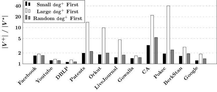We show $\frac{\textnormal{sum of }|V^{+}|\textnormal{ over all insertions}}{\textnormal{sum of }|V^{*}|\textnormal{ over all insertions}}$ for three heuristics in Figure 9 after inserting 100,000 edges. From the figure, we can see that the “small ${\mathsf{deg}}^{+}$ first” heuristic consistently performs better in all $11$ graphs tested.

Figure 9: Comparison of Heuristics to Generate the $k$-Order

Implementation: In order to traverse $O_{k}$ efficiently, $O_{k}$ is implemented as a doubly linked list. Recall that we associate $O_{k}$ with a data structure $\mathcal{A}_{k}$ to test $u\preceq v$ when both are in $O_{k}$. In addition, we use a data structure $\mathcal{B}$ such that jumping to $v_{j}$ (line 2 of Algorithm 2) takes $\mathcal{O}(1)$ time. In order to make both $\mathsf{OrderInsert}$ (Algorithm 2) and $\mathsf{OrderRemoval}$ (Algorithm 4) efficient, there are two main issues: (A) how to implement $\mathcal{A}_{k}$, and (B) how to implement $\mathcal{B}$.

(A) How to implement $\mathcal{A}_{k}$: Here, the data structure is needed to test $u\preceq v$ when both are in the same $O_{k}$; that is, ${\mathsf{core}}(u)={\mathsf{core}}(v)$. On selecting an appropriate data structure for such a purpose, we take the following observation into consideration.

Observation 6.1: In algorithm $\mathsf{OrderInsert}$, it is possible that $u\preceq v$ in the $k$-order $\preceq$ of $G$ is changed to $v\preceq^{\prime}u$ in the new order $\preceq^{\prime}$ after $G$ is updated by inserting/removing an edge.

We explain how it happens. Consider processing vertices in $O_{k}$ from left to right one-by-one as an example. Suppose $u\preceq v$. Initially, suppose $u$ is in Case-1. As a result, by the $\mathsf{OrderInsert}$ algorithm, $u$ is appended to $V_{C}$ instead of $O^{\prime}_{K}$ as a candidate to be in $V^{*}$. While $u$ is in $V_{C}$, the $\mathsf{OrderInsert}$ algorithm processes $v$, finds that $v$ is in Case-2, and thus appends $v$ to $O^{\prime}_{K}$. Some time later, it is possible that $u$ is found not to be a candidate any more when the algorithm processes a vertex $w$, which is in Case-2b. Note that $w$ may be $v$. Then $u$ is removed from $V_{C}$ and also appended to $O^{\prime}_{K}$. This causes $v\preceq^{\prime}u$ in the new $k$-order $\preceq^{\prime}$. We emphasize that there are at most $|V^{+}|$ such $u$s on a single edge insertion because $V^{+}$ includes all vertices that are in Case-1 in the $\mathsf{OrderInsert}$ algorithm. We discuss how to support $\mathcal{A}_{k}$ below.

In current implementation, we encode $\mathcal{A}_{k}$ using an order statistics tree, where each tree node holds exactly one vertex. The following invariant is maintained: for any two vertices $u$ and $v$ in $O_{k}$, if $u\preceq v$, then (1) $u$ is in the left subtree of $v$, or (2) $v$ is in the right subtree of $u$, or (3) there exists $w\in O_{k}$ such that $u$ is in the left subtree of $w$ and $v$ is in the right subtree of $w$. By associating each node with the size of the subtree rooted at the node, we are able to find the rank of a vertex in $O_{k}$ in $\mathcal{O}(\log|O_{k}|)$ time [7]. Such a method faces an issue. Given an order statistics tree, in order to find the rank of a vertex, we need to first locate the node containing the vertex, starting from the root. But we cannot decide which child pointer to follow to find the node, since we do not have the rank information yet. In other words, given a vertex, in order to get the rank of the vertex using the tree, we should first know the rank of the vertex. We propose a mechanism to address this issue by additionally creating a one-to-one mapping between vertices in $O_{k}$ and nodes in the order statistics tree. In this way, locating the target node in the order statistics tree can be done easily. It is worth noting that in our algorithm, vertices are inserted either to the beginning of $O_{K+1}$ for insertion or the end of $O_{K-1}$ for removal. Accordingly, we only need to follow either the left child pointers or the right child pointers to insert the vertex to the order statistics tree. Therefore, the issue mentioned above is avoided. The post-processing to make the tree balanced is similar to that of an ordinary tree. Both insertion and removal of a vertex takes $\mathcal{O}(\log|O_{k}|)$ time.

We show below that $\mathcal{A}_{k}$s deal with Observation 9 well. To make it consistent with the new $k$-order $O^{\prime}_{k}$, we adjust the position of $u$ (refer to Observation 9) in the order statistics tree as follows. First, we remove $u$ from the tree. Suppose $u^{\prime}$ is the previous vertex of $u$ in $O^{\prime}_{k}$. We insert $u$ to the right subtree of $u^{\prime}$ by following only left child pointers such that $u$ is the successor of $u^{\prime}$ in the tree. Local rotations are then taken to make the tree valid. The total cost for adjusting positions thus is $\mathcal{O}(|V^{+}|\log|O_{k}|)$ because there are at most $|V^{+}|$ such $u$s and each takes $\mathcal{O}(\log|O_{k}|)$ time. This additional cost does not affect the complexity of Theorem 3.

Theorem 6.1: The total space cost of $\mathcal{A}_{k}$s is $\mathcal{O}(n)$ and for each $k$, $\mathcal{A}_{k}$ can be created in $\mathcal{O}(|O_{k}|\log|O_{k}|)$ time by inserting vertices in $O_{k}$ one by one.

(B) How to implement $\mathcal{B}$: $\mathcal{B}$ is implemented as a min-heap. $\mathcal{B}$ maintains a set of (${\mathsf{rank}}(w)$, $w$) pairs with ${\mathsf{deg}}^{*}(w)\neq 0$ or ${\mathsf{deg}}^{+}(w)$ $>K$ (Case-1 and Case-2b), and uses the rank as the key. When we need to find the $v_{j}$ (line 2 of Algorithm 2), the top pair of $\mathcal{B}$ is returned in $\mathcal{O}(1)$ time. It requires $\mathcal{O}(\log|\mathcal{B}|)=\mathcal{O}(\log|O_{K}|)$ time to insert a pair to $\mathcal{B}$ since only vertices in $O_{K}$ will be inserted to $\mathcal{B}$. It requires $\mathcal{O}(\log|\mathcal{B}|)$ time to remove arbitrary pair from $\mathcal{B}$.

VII Performance Studies

We have conducted experimental studies using 11 real large graphs, and we report the performance of our algorithms by comparing with the traversal algorithms. All algorithms are implemented in C++ and compiled by g++ compiler at -O2 optimization level. For the new order-based algorithms, we implement the order statistics tree on top of treaps. For the traversal algorithms, we apply the enhancement proposed in [14], which is the journal version of [13]. The enhancement consists of exploiting neighborhood of higher hops to improve the pruning power of ${\mathsf{pcd}}$, which considers only $2$-hop neighborhood of a vertex, at a higher maintenance cost. Note that the traversal removal algorithm requires only ${\mathsf{mcd}}$ and thus its performance degrades for higher hops. We set the hop count $h$ in the range $\{2,3,4,5,6\}$ as in [14] and denote each version as ${\mathsf{Trav}}\textnormal{-}h$. All experiments are conducted on a Linux machine with Intel i7-4790 CPU and 32 GB main memory.

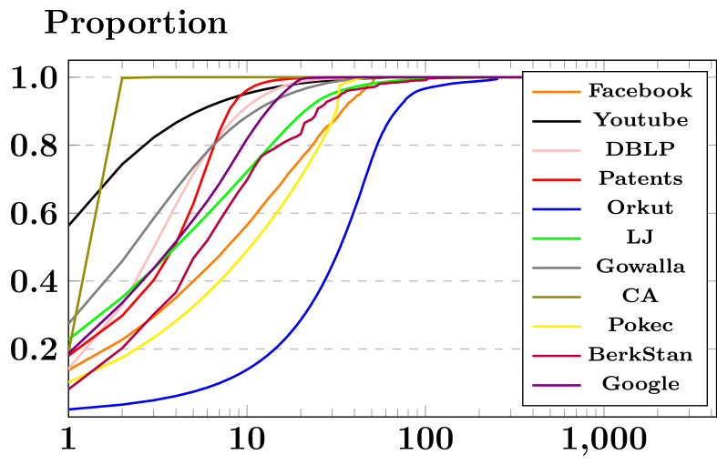
Datasets: We use $11$ datasets publicly accessible, which are shown in Table I. These real datasets cover a wide range of graphs used in different applications with different properties. $\mathsf{Facebook}$, $\mathsf{Youtube}$, and $\mathsf{DBLP}$ are three temporal graphs, whose edges are labeled with time stamps to show when they are inserted, and can be downloaded from Konect (http://konect.uni-koblenz.de). The remaining eight graphs, which can be downloaded from SNAP (https://snap.stanford.edu), include Social Networks ($\mathsf{LiveJournal}$, $\mathsf{Pokec}$, and $\mathsf{Orkut}$), Citation Network ($\mathsf{Patents}$), Web Graphs ($\mathsf{BerkStan}$ and $\mathsf{Google}$), Road Network ($\mathsf{CA}$), and Location-Based Social Network ($\mathsf{Gowalla}$). Directed graphs are converted to undirected ones in our testing. The statistics are shown in Table I. The cumulative distribution of core numbers for each graph is shown in Figure 10(a).

Dataset	$n=|V|$	$m=|E|$	avg. $\mathsf{deg}$	max $k$
$\mathsf{Facebook}$	63,731	817,035	25.64	52
$\mathsf{Youtube}$	3,223,589	9,375,374	5.82	88
$\mathsf{DBLP}$	1,314,050	5,362,414	8.16	118
$\mathsf{Patents}$	3,774,768	16,518,947	8.75	64
$\mathsf{Orkut}$	3,072,441	117,185,083	76.28	253
$\mathsf{LiveJournal}$	4,846,609	42,851,237	17.68	372
$\mathsf{Gowalla}$	196,591	950,327	9.67	51
$\mathsf{CA}$	1,965,206	2,766,607	2.82	3
$\mathsf{Pokec}$	1,632,803	22,301,964	27.32	47
$\mathsf{BerkStan}$	685,230	6,649,470	19.41	201
$\mathsf{Google}$	875,713	4,322,051	9.87	44

TABLE I: Datasets

(a) The cumulative distribution of core numbers

(b) Cumulative distribution of $K$ of the 100,000 edges sampled

Figure 10: Statistics of the Graphs and Edges Tested

VII-A Order-Based vs Traversal

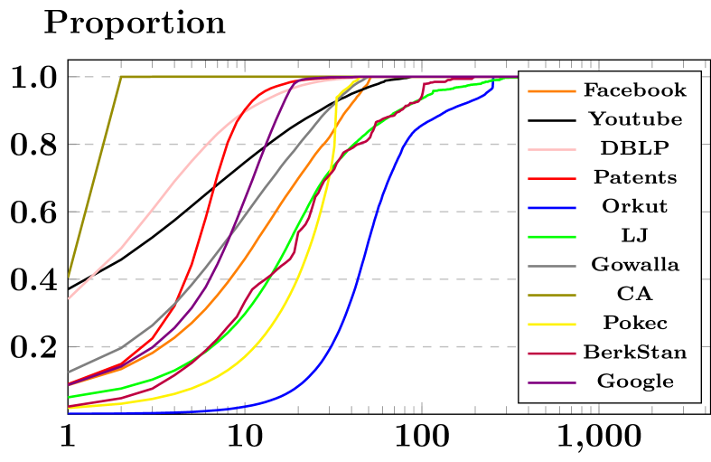
We compare the performance of our order-based algorithms with the traversal algorithms, which are the state-of-the-art. Here, we select 100,000 edges out of each of the 11 graphs as follows. For the three graphs with time stamps on edges, $\mathsf{Facebook}$, $\mathsf{Youtube}$ and $\mathsf{DBLP}$, because each edge is associated with a time stamp, we select the latest 100,000 edges, i.e., the edges with maximum time stamps. For each of the remaining eight graphs, we randomly sample 100,000 edges. For each graph, we show the cumulative distribution of $K$ of the 100,000 edges sampled in Figure 10(b), where $K=\min\{{\mathsf{core}}(u),{\mathsf{core}}(v)\}$ given an edge $(u,v)$. Figure 10(b) shows that the edges to test cover $k$-cores in wide range, implying they are suitable for testing. For each graph, we measure the accumulated time for inserting these 100,000 edges one by one, and then measure the accumulated time for removing these edges from the graph. The results are shown in TABLE II.

Edge Insertion: We compare $\mathsf{OrderInsert}$ (Algorithm 2) with the traversal insertion algorithm [13] ([14]). The results are shown in TABLE II. $\mathsf{OrderInsert}$ significantly outperforms the traversal insertion algorithm in all the datasets tested. For $\mathsf{Pokec}$, the speedup even achieves up to 2,083 times. For $\mathsf{Patents}$ and $\mathsf{CA}$, we further test with higher $h$ for the traversal insertion algorithm to get the optimal efficiency and the results are 810.00s ($h=6$) for $\mathsf{Patents}$ and 1.08s ($h=7$) for $\mathsf{CA}$, which are still slower than $\mathsf{OrderInsert}$. As shown in Figure 2, $\mathsf{OrderInsert}$ visits much less vertices than ${\mathsf{Trav}}\textnormal{-}2$. This confirms the efficiency of $\mathsf{OrderInsert}$ algorithm. In addition, we emphasize that $\mathsf{OrderInsert}$ has much smaller performance variation between edges inserted, as shown in Figure 1.

	Insert						Remove
Dataset	$\mathsf{OrderInsert}$	$\mathsf{Trav}$-2	$\mathsf{Trav}$-3	$\mathsf{Trav}$-4	$\mathsf{Trav}$-5	$\mathsf{Trav}$-6	$\mathsf{OrderRemoval}$	$\mathsf{Trav}$-2	$\mathsf{Trav}$-3	$\mathsf{Trav}$-4	$\mathsf{Trav}$-5	$\mathsf{Trav}$-6
$\mathsf{Facebook}$	0.16	3.52	4.07	5.91	10.52	16.95	0.10	0.50	1.63	4.14	9.70	17.77
$\mathsf{Youtube}$	0.26	2.51	2.88	4.01	6.13	9.71	0.28	0.61	1.42	3.19	6.28	11.32
$\mathsf{DBLP}$	0.16	1.80	1.20	2.31	6.32	17.65	0.11	0.21	0.61	1.88	5.49	15.78
$\mathsf{Patents}$	0.88	2,944.14	1,805.98	1,173.20	845.93	810.00	0.38	0.92	4.22	18.57	75.06	276.37
$\mathsf{Orkut}$	1.14	954.36	793.82	780.69	996.43	1,576.63	0.71	7.75	36.80	136.78	428.85	1,089.38
$\mathsf{LiveJournal}$	0.53	149.56	90.93	76.57	125.29	285.50	0.33	1.66	6.59	24.56	86.10	233.92
$\mathsf{Gowalla}$	0.18	1.04	1.37	2.21	3.78	6.38	0.14	0.35	0.84	1.82	3.45	6.22
$\mathsf{CA}$	0.52	15.14	4.20	2.08	1.37	1.11	0.16	0.08	0.13	0.19	0.26	0.33
$\mathsf{Pokec}$	0.77	1,726.04	1,603.80	1,650.37	1,876.48	2,338.78	0.32	4.86	53.13	259.93	756.40	1,652.88
$\mathsf{BerkStan}$	0.37	6.37	7.29	9.37	13.14	16.19	0.52	2.55	5.04	8.33	12.45	17.34
$\mathsf{Google}$	0.37	1.01	1.25	2.44	4.81	9.27	0.25	0.46	0.96	2.08	4.32	8.75

TABLE II: Performance Comparison (in seconds): Order-Based vs Traversal (The winner is in bold; the runner-up is in italics)

Edge Removal: We compare $\mathsf{OrderRemoval}$ (Algorithm 4) with the traversal removal algorithm [13] ([14]). The results are shown in TABLE II. We observe that ${\mathsf{Trav}}\textnormal{-}2$ is more efficient than those with higher $h$, and $\mathsf{OrderRemoval}$ outperforms ${\mathsf{Trav}}\textnormal{-}2$ in all datasets except $\mathsf{CA}$. Here, the average degree of $\mathsf{CA}$ is only $2.82~{}{}(\approx 3)$, as shown in TABLE I. Such a small average degree indicates that the cost to maintain ${\mathsf{pcd}}$ is low, because the number of vertices whose ${\mathsf{pcd}}$ need to be updated after an edge update is small. On the other hand, $\mathsf{OrderRemoval}$ outperforms ${\mathsf{Trav}}\textnormal{-}2$ in all other graphs tested, especially $\mathsf{Pokec}$ and $\mathsf{Orkut}$, because $\mathsf{Pokec}$ and $\mathsf{Orkut}$ have the highest average degrees among all the datasets.

Index Space and Index Creation: Our order-based algorithm requires $\mathcal{O}(n)$ space, as shown in Theorem 9. In our current implementation, the order-based algorithm needs about five times of the space used by ${\mathsf{Trav}}\textnormal{-}2$ and needs only about double time to create the index (including computing the initial core numbers). When the hop count $h$ becomes larger, the space and time required by the traversal algorithms also become higher. See TABLE III. We emphasize that index creation is a one-time cost. Moreover, in view of the insertion/removal performance improvement brought, such a tradeoff is appropriate.

(a) Vary $|V|$: time

(b) Vary $|V|$: edge ratio

(c) Vary $|E|$: time

(d) Vary $|E|$: vertex ratio

Figure 11: The Scalability of the $\mathsf{OrderInsert}$ Algorithm

VII-B Scalability Testing

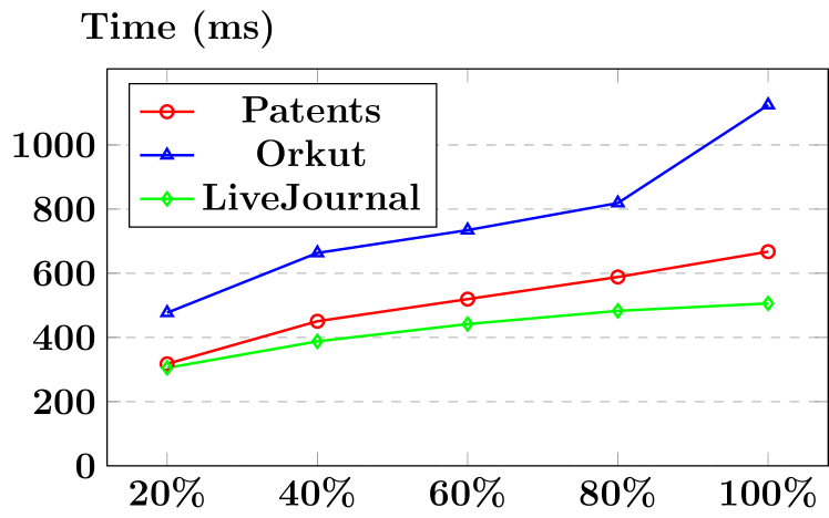
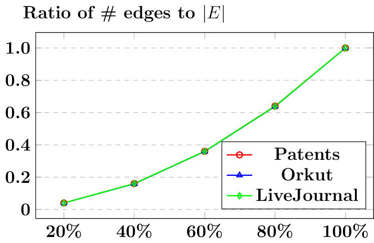
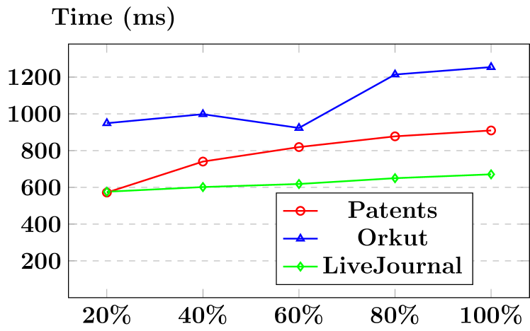
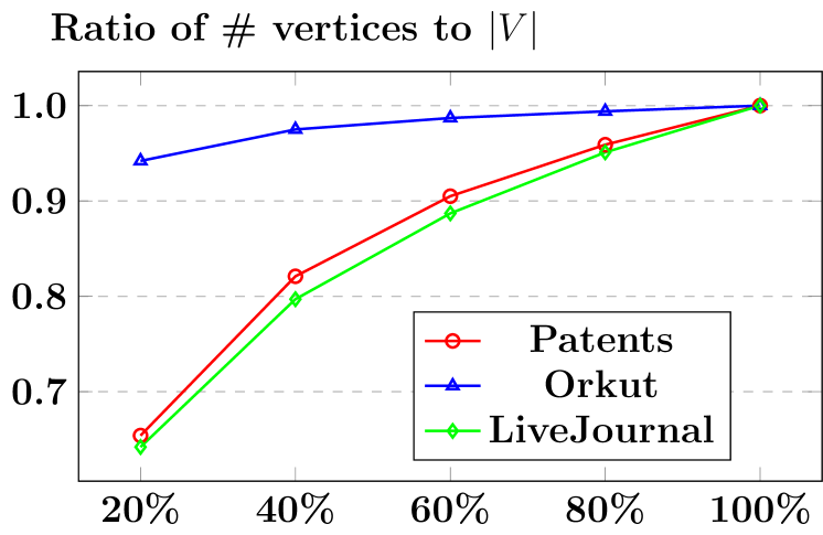
We test the scalability of $\mathsf{OrderInsert}$ using the largest three datasets, i.e., $\mathsf{Patents}$, $\mathsf{Orkut}$, and $\mathsf{LiveJournal}$. We vary the number of vertices $|V|$ and the number of edges $|E|$ respectively by randomly sampling vertices and edges at rates from 20% to 100%. When sampling vertices, we use the subgraph induced by the vertices. When sampling edges, we keep the incident vertices of the edges. From each subgraph sampled, we further sample 100,000 edges for testing. We show the results in Figure 11. Figure 11(a) shows the total time (ms) to insert the sampled 100,000 edges one by one and update core numbers, and Figure 11(b) shows the ratio of the number of edges in each sampled subgraph to the number of edges in the original graph, while varying $|V|$. As can be seen, the time taken by $\mathsf{OrderInsert}$ grows smoothly while the number of edges increase rapidly. Figure 11(c) shows the total time (ms) to insert the sampled 100,000 edges and update core numbers, and Figure 11(d) shows the ratio of the number of vertices in each sampled subgraph to the number of vertices in the original graph, while varying $|E|$. Similarly, $\mathsf{OrderInsert}$ performs well while the number of vertices increase rapidly. We do not show the scalability results for $\mathsf{OrderRemoval}$ because it only relies on $V^{*}$ and their neighbors, as shown in Theorem V-C. The scalability thus is not an issue of $\mathsf{OrderRemoval}$.

VII-C Stability Testing

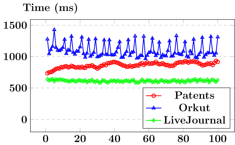
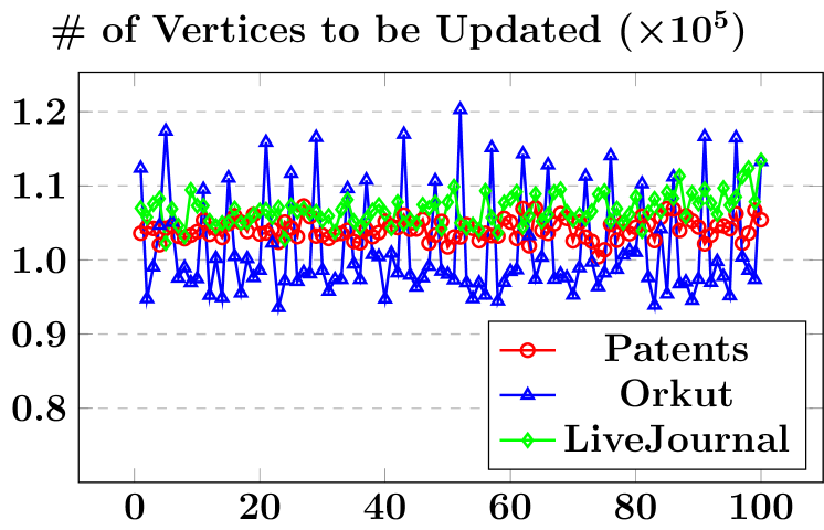
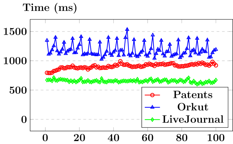
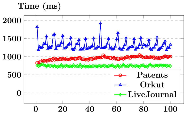
We update the $k$-order when an edge inserted. An issue is whether the effectiveness of the $k$-order will be stable after a large number of edge insertions. We test the stability of the algorithm using the largest three datasets, i.e., $\mathsf{Patents}$, $\mathsf{Orkut}$, and $\mathsf{LiveJournal}$. The stability testing is conducted as follows. First, we randomly sample 10,000,000 edges from the graph and randomly partition them into 100 groups, where each group has 100,000 edges. Second, we reinsert these edges to the graph group by group. For each group, we measure the accumulated time used by $\mathsf{OrderInsert}$ to insert the edges one by one. Figure 12(a) shows the results. The performance of the $\mathsf{OrderInsert}$ insertion algorithm is well bounded, for all three datasets. For $\mathsf{Orkut}$ graph, we observe that its result fluctuates frequently. This is due to the fact that the number of vertices whose core numbers need to be updated inside each group varies a lot, as can be seen in Figure 12(b). To make the experiment more practical, we conducted two additional experiments as follows. For each group, after an edge is inserted, with probability $p$ we randomly remove an edge from the graph. In the experiments, we set $p$ as $0.1$ and $0.2$ respectively and the total time measured also includes the time of removing edges. The results are similar to Figure 12(a), as shown in Figure 12(c) and 12(d).

(a) $p=0$

(b) # of Vertices to be Updated

(c) $p=0.1$

(d) $p=0.2$

Figure 12: The Stability of the $\mathsf{OrderInsert}$ Algorithm

VIII Conclusions

In this paper, we study core maintenance to reduce the computational cost to compute $k$-cores for a graph when edges are inserted/removed dynamically. To further improve the efficiency of the state-of-the-art traversal algorithm, we propose a new order-based algorithm. The key is to explicitly maintain the $k$-order for a graph. With the $k$-order, we can identify the set of vertices that need to be updated efficiently, and we can maintain the $k$-order for a graph with small overhead when edges are inserted/removed. We confirm our approach by conducting extensive performance studies using 11 real large graphs. Our $\mathsf{OrderInsert}$ algorithm outperforms the traversal insertion algorithm up to 3 orders of magnitude.

[Proof of Theorems and Lemmas]

Proof Sketch of Lemma V The if part: In Algorithm 1, if vertices are removed in the order $O_{0}O_{1}O_{2}\cdots$, it is guaranteed that the remaining degree of a vertex $v$ is ${\mathsf{deg}}^{+}(v)<k+1$, when $v$ is the current vertex being processed. Thus, $v$ can be removed. The only if part: this is trivial and omitted.

Proof Sketch of Lemma V-B We have ${\mathsf{deg}}^{+}(w)\leq K$ for $\forall w\in O_{K}$ if ${\mathsf{deg}}^{+}(u)\leq K$. Let $w$ be the first vertex in $O_{K}$. The number of $w$’s neighbors in the $(K+1)$-core of $G^{\prime}$ is at most ${\mathsf{deg}}^{+}(w)\leq K$. Thus, $w$ can not be in the $(K+1)$-core of $G^{\prime}$. We can infer similarly for remaining vertices in $O_{K}$.

Proof Sketch of Lemma V-B After $(u,v)$ is inserted, ${\mathsf{deg}}^{+}(w)$ for the vertex $w$ appearing before $u$ will remain unchanged, i.e., $\leq K$. The proof is similar to that of Lemma V-B and is thus omitted.

Proof Sketch of Theorem 3 The preparing phase is in $\mathcal{O}(\log|O_{K}|)$ time because we need to test whether $u\preceq v$, using $\mathcal{A}_{K}$. The main part of the core phase is the while loop (lines 2-2). First, the algorithm enters the second branch (lines 2-2) in the while loop at most $|V^{+}|+1$ times. Because lines 2-2 take $\mathcal{O}(1)$ time using $\mathcal{B}$, the total time complexity for this branch in the whole loop is $\mathcal{O}(|V^{+}|)$. Second, lines 2-2 take $\mathcal{O}({\mathsf{deg}}(v_{i})\log|O_{K}|)$ time, because we need to enumerate neighbors of $v_{i}$ and for each neighbor $w$, we test $v_{i}\preceq w$. In total, this branch takes $\mathcal{O}(\log|O_{K}|\cdot\sum_{v\in V^{+}}{\mathsf{deg}}(v))$ time during the whole loop. Third, the third branch (lines 2-2) takes $\mathcal{O}(\sum_{v\in V^{+}}{\mathsf{deg}}(v)\log|O_{K}|)$ time in total in the whole loop. Note that Algorithm 3 is called to remove more vertices from $V_{C}$ each time when the algorithm enters this branch. Each vertex $w^{\prime}$ that is removed from $V_{C}$ takes $\mathcal{O}({\mathsf{deg}}(w^{\prime})\log|O_{K}|)$ time to update ${\mathsf{deg}}^{+}$ and ${\mathsf{deg}}^{*}$ and to find more vertices to remove. There are at most $|V^{+}|$ such $w^{\prime}$s in the whole loop because $w^{\prime}$ must be in Case-1 for it to be inserted to $V_{C}$. For the ending phase, because $V^{*}\subseteq V^{+}$, updating ${\mathsf{mcd}}$ takes $\mathcal{O}(\sum_{v\in V^{*}}{\mathsf{deg}}(v))=\mathcal{O}(\sum_{v\in V^{+}}{\mathsf{deg}}(v))$. In addition, it takes $\mathcal{O}(|V^{*}|\log\max\{|O_{K}|,|O_{K+1}|\})$ time to move vertices between $\mathcal{A}_{K}$ and $\mathcal{A}_{K+1}$. Thus, the complexity of Algorithm 2 is $\mathcal{O}((\sum_{v\in V^{+}}{\mathsf{deg}}(v))\cdot\log\max\{|O_{K}|,\linebreak|O_{K+1}|\})$.

Proof Sketch of Theorem V-C For vertices that are still in $O_{K}$, their ${\mathsf{deg}}^{+}$s are not increased in the algorithm. Thus, their ${\mathsf{deg}}^{+}$ remains smaller than or equal to $K$. Let the vertices in $V^{*}$ be $w_{1},w_{2},\cdots,w_{|V^{*}|}$ in the order they are inserted to $V^{*}$. The traversal removal algorithm guarantees that when we insert a vertex $w_{i}$ to $V^{*}$, ${\mathsf{deg}}(w_{i},G(V_{\geq K}\setminus\{w_{1},w_{2},\cdots,w_{i-1}\}))\leq K-1$, where $V_{\geq K}$ is the original set of vertices whose core numbers are not less than $K$. Therefore, we have ${\mathsf{deg}}^{+}(w_{i})\leq K-1$ for each $w_{i}\in V^{*}$.

Proof Sketch of Theorem V-C First, identifying $V^{*}$ takes only $\mathcal{O}(\sum_{w\in V^{*}}{\mathsf{deg}}(w))$ time. Second, maintaining $O_{K}$ and $O_{K-1}$ requires $\mathcal{O}(\log|O_{K}|\cdot\sum_{w\in V^{*}}{\mathsf{deg}}_{K}(w)+|V^{*}|\cdot\log|O_{K-1}|)$ time. We provide the analysis below for each $w\in V^{*}$. (a) Lines 4-4 totally take $\mathcal{O}({\mathsf{deg}}(w)+{\mathsf{deg}}_{K}(w)\log|O_{K}|)$ time. Note that $w^{\prime}\preceq w$ is evaluated only if ${\mathsf{core}}(w^{\prime})=K$. (b) Lines 4-4 totally take $\mathcal{O}({\mathsf{deg}}(w))$ time assuming testing $w^{\prime}\in V^{*}$ requires $\mathcal{O}(1)$ time. (c) Lines 4-4 require $\mathcal{O}(1)+\mathcal{O}(\log|O_{K}|+\log|O_{K-1}|)$ time, where $\mathcal{O}(1)$ is for removing $w$ from $V^{*}$ and moving $w$ from $O_{K}$ to $O_{K-1}$, while $\mathcal{O}(\log|O_{K}|+\log|O_{K-1}|)$ is for removing $w$ from $\mathcal{A}_{K}$ and inserting $w$ to $\mathcal{A}_{K-1}$. In addition, line 4 requires $\mathcal{O}(\sum_{v\in V^{*}}{\mathsf{deg}}(v))$ time.

[Index Creation Time Comparison]

Dataset	Order-Based	$\mathsf{Trav}$-2	$\mathsf{Trav}$-3	$\mathsf{Trav}$-4	$\mathsf{Trav}$-5	$\mathsf{Trav}$-6
$\mathsf{Facebook}$	0.03	0.03	0.03	0.04	0.05	0.06
$\mathsf{Youtube}$	1.45	0.96	1.14	1.33	1.50	1.69
$\mathsf{DBLP}$	0.74	0.54	0.65	0.77	0.85	0.95
$\mathsf{Patents}$	3.93	3.65	4.32	5.03	5.76	6.32
$\mathsf{Orkut}$	7.25	7.39	9.16	10.90	12.91	14.49
$\mathsf{LiveJournal}$	4.26	3.75	4.63	5.53	6.23	7.14
$\mathsf{Gowalla}$	0.07	0.06	0.07	0.09	0.10	0.11
$\mathsf{CA}$	0.77	0.35	0.43	0.50	0.58	0.64
$\mathsf{Pokec}$	2.49	2.67	3.02	3.33	3.90	4.11
$\mathsf{BerkStan}$	0.32	0.29	0.37	0.44	0.51	0.58
$\mathsf{Google}$	0.45	0.35	0.44	0.52	0.59	0.66

TABLE III: Time to Create Index (in seconds)

References

- [1] H. Aksu, M. Canim, Y.-C. Chang, I. Korpeoglu, and O. Ulusoy. Distributed-core view materialization and maintenance for large dynamic graphs. IEEE TKDE, 26(10), 2014.
- [2] J. I. Alvarez-Hamelin, L. Dall Asta, A. Barrat, and A. Vespignani. How the k-core decomposition helps in understanding the internet topology. In ISMA Workshop on the Internet Topology, volume 1, 2006.
- [3] J. I. Alvarez-Hamelin, L. Dall’Asta, A. Barrat, and A. Vespignani. Large scale networks fingerprinting and visualization using the k-core decomposition. In Proc. of NIPS’06, 2006.
- [4] V. Batagelj and M. Zaversnik. An o(m) algorithm for cores decomposition of networks. arXiv preprint cs/0310049, 2003.
- [5] J. Cheng, Y. Ke, S. Chu, and M. T. Özsu. Efficient core decomposition in massive networks. In Proc. of ICDE’11, 2011.
- [6] J. Cohen. Trusses: Cohesive subgraphs for social network analysis. National Security Agency Technical Report, page 16, 2008.
- [7] T. H. Cormen, C. E. Leiserson, R. L. Rivest, and C. Stein. Introduction to Algorithms. MIT Press, 2009.
- [8] A. Epasto, S. Lattanzi, and M. Sozio. Efficient densest subgraph computation in evolving graphs. In Proc. of WWW’15, 2015.
- [9] W. Fan, J. Li, J. Luo, Z. Tan, X. Wang, and Y. Wu. Incremental graph pattern matching. In Proc. of SIGMOD’11, 2011.
- [10] W. Khaouid, M. Barsky, V. Srinivasan, and A. Thomo. K-core decomposition of large networks on a single pc. PVLDB, 9(1), 2016.
- [11] R.-H. Li, J. X. Yu, and R. Mao. Efficient core maintenance in large dynamic graphs. IEEE TKDE, 26(10), 2014.
- [12] A. Montresor, F. De Pellegrini, and D. Miorandi. Distributed k-core decomposition. IEEE TPDS, 24(2), 2013.
- [13] A. E. Sariyüce, B. Gedik, G. Jacques-Silva, K.-L. Wu, and Ü. V. Çatalyürek. Streaming algorithms for k-core decomposition. PVLDB, 6(6), 2013.
- [14] A. E. Sariyüce, B. Gedik, G. Jacques-Silva, K.-L. Wu, and Ü. V. Çatalyürek. Incremental k-core decomposition: algorithms and evaluation. VLDBJ, 25(3), 2016.
- [15] J. Wang and J. Cheng. Truss decomposition in massive networks. PVLDB, 5(9), 2012.
- [16] D. Wen, L. Qin, Y. Zhang, X. Lin, and J. X. Yu. I/o efficient core graph decomposition at web scale. In Proc. of ICDE’16, 2016.
- [17] H. Zhang, H. Zhao, W. Cai, J. Liu, and W. Zhou. Using the k-core decomposition to analyze the static structure of large-scale software systems. The Journal of Supercomputing, 53(2), 2010.
- [18] A. D. Zhu, W. Lin, S. Wang, and X. Xiao. Reachability queries on large dynamic graphs: A total order approach. In Proc. of SIGMOD’14, 2014.