Neural Network Translation Models for Grammatical Error Correction

Abstract

Phrase-based statistical machine translation (SMT) systems have previously been used for the task of grammatical error correction (GEC) to achieve state-of-the-art accuracy. The superiority of SMT systems comes from their ability to learn text transformations from erroneous to corrected text, without explicitly modeling error types. However, phrase-based SMT systems suffer from limitations of discrete word representation, linear mapping, and lack of global context. In this paper, we address these limitations by using two different yet complementary neural network models, namely a neural network global lexicon model and a neural network joint model. These neural networks can generalize better by using continuous space representation of words and learn non-linear mappings. Moreover, they can leverage contextual information from the source sentence more effectively. By adding these two components, we achieve statistically significant improvement in accuracy for grammatical error correction over a state-of-the-art GEC system.

1 Introduction

Grammatical error correction (GEC) is a challenging task due to the variability of the type of errors and the syntactic and semantic dependencies of the errors on the surrounding context. Most of the grammatical error correction systems use classification and rule-based approaches for correcting specific error types. However, these systems use several linguistic cues as features. The standard linguistic analysis tools like part-of-speech (POS) taggers and parsers are often trained on well-formed text and perform poorly on ungrammatical text. This introduces further errors and limits the performance of rule-based and classification approaches to GEC. As a consequence, the phrase-based statistical machine translation (SMT) approach to GEC has gained popularity because of its ability to learn text transformations from erroneous text to correct text from error-corrected parallel corpora without any additional linguistic information. They are also not limited to specific error types. Currently, many state-of-the-art GEC systems are based on SMT or use SMT components for error correction Susanto et al. (2014); Felice et al. (2014); Junczys-Dowmunt and Grundkiewicz (2014). In this paper, grammatical error correction includes correcting errors of all types, including word choice errors and collocation errors which constitute a large class of learners’ errors.

We model our GEC system based on the phrase-based SMT approach. However, traditional phrase-based SMT systems treat words and phrases as discrete entities. We take advantage of continuous space representation by adding two neural network components that have been shown to improve SMT systems Ha et al. (2014); Devlin et al. (2014). These neural networks are able to capture non-linear relationships between source and target sentences and can encode contextual information more effectively. Our experiments show that the addition of these two neural networks leads to significant improvements over a strong baseline and outperforms the current state of the art.

2 Related Work

In the past decade, there has been increasing attention on grammatical error correction in English, mainly due to the growing number of English as Second Language (ESL) learners around the world. The popularity of this problem in natural language processing research grew further through Helping Our Own (HOO) and the CoNLL shared tasks Dale and Kilgarriff (2011); Dale et al. (2012); Ng et al. (2013, 2014). Most published work in GEC aimed at building specific classifiers for different error types and then use them to build hybrid systems Dahlmeier et al. (2012); Rozovskaya et al. (2014). One of the first approaches of using SMT for GEC focused on correction of countability errors of mass nouns (e.g., many informations$\rightarrow$much information) Brockett et al. (2006). They had to use an artificially constructed parallel corpus for training their SMT system. Later, the availability of large-scale error corrected data Mizumoto et al. (2011) further improved SMT-based GEC systems.

Recently, continuous space representations of words and phrases have been incorporated into SMT systems via neural networks. Specifically, addition of monolingual neural network language models Bengio et al. (2003); Vaswani et al. (2013), neural network joint models (NNJM) Devlin et al. (2014), and neural network global lexicon models (NNGLM) Ha et al. (2014) have been shown to be useful for SMT. Neural networks have been previously used for GEC as a language model feature in the classification approach Wu et al. (2014) and as a classifier for article error correction Sun et al. (2015). Recently, a neural machine translation approach has been proposed for GEC Yuan and Briscoe (2016). This method uses a recurrent neural network to perform sequence-to-sequence mapping from erroneous to well-formed sentences. Additionally, it relies on a post-processing step based on statistical word-based translation models to replace out-of-vocabulary words. In this paper, we investigate the effectiveness of two neural network models, NNGLM and NNJM, in SMT-based GEC. To the best of our knowledge, there is no prior work that uses these two neural network models for SMT-based GEC.

3 A Machine Translation Framework for Grammatical Error Correction

In this paper, the task of grammatical error correction is formulated as a translation task from the language of ‘bad’ English to the language of ‘good’ English. That is, the source sentence is written by a second language learner and potentially contains grammatical errors, whereas the target sentence is the corrected fluent sentence. We use a phrase-based machine translation framework Koehn et al. (2003) for translation, which employs a log-linear model to find the best translation $T^{*}$ given a source sentence $S$. The best translation is selected according to the following equation:

$$T^{*}=\operatorname*{argmax}_{T}P(T|S)=\operatorname*{argmax}_{T}\sum_{i=1}^{N}\lambda_{i}h_{i}(T,S)$$

where $N$ is the number of features, $h_{i}$ and $\lambda_{i}$ are the $i$^th feature function and feature weight, respectively. We make use of the standard features used in phrase-based translation without any reordering, leading to monotone translations. The features can be broadly categorized as translation model and language model features. The translation model in the phrase-based machine translation framework is trained using parallel data, i.e., sentence-aligned erroneous source text and corrected target text. The translation model is responsible for finding the best transformation of the source sentence to produce the corrected sentence. On the other hand, the language model is trained on well-formed English text and this ensures the fluency of the corrected text. To find the optimal feature weights ($\lambda$), we use minimum error rate training (MERT), maximizing the $F_{0.5}$ measure on the development set Junczys-Dowmunt and Grundkiewicz (2014). The $F_{0.5}$ measure Dahlmeier and Ng (2012), which weights precision twice as much as recall, is the evaluation metric widely used for GEC and was the official evaluation metric adopted in the CoNLL 2014 shared task Ng et al. (2014).

Additionally, we augment the feature set by adding two neural network translation models, namely a neural network global lexicon model Ha et al. (2014) and a neural network joint model Devlin et al. (2014). These models are described in detail in Sections 4 and 5.

4 Neural Network Global Lexicon Model

A global lexicon model is used to predict the presence of words in the corrected output. The model estimates the overall probability of a target hypothesis (i.e., a candidate corrected sentence) given the source sentence, by making use of the probability computed for each word in the hypothesis. The individual word probabilities can be computed by training density estimation models such as maximum entropy Mauser et al. (2009) or probabilistic neural networks Ha et al. (2014). Following Ha et al. (2014), we formulate our global lexicon model using a feed-forward neural network. The model and the training algorithm are described below.

4.1 Model

The probability of a target hypothesis is computed using the following equation:

$$P(T|S)\approx\prod_{i=1}^{|T|}P(t_{i}|S)$$ (1)

where $S$ and $T$ are the source sentence and the target hypothesis respectively, and $|T|$ denotes the number of words in the target hypothesis. $P(t_{i}|S)$ is the probability of the target word $t_{i}$ given the source sentence $S$. $P(t_{i}|S)$ is the output of the neural network. The architecture of the neural network is shown in Figure 1. $P(t_{i}|S)$ is calculated by:

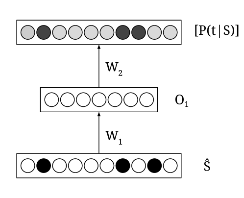
Figure 1: A single hidden layer neural network global lexicon model

$$P(t_{i}|S)=\sigma_{i}(W_{2}\cdot O_{1}+b_{2})$$

where $O_{1}$ is the hidden layer output, and $W_{2}$ and $b_{2}$ are the output layer weights and biases respectively. $\sigma_{i}$ is the element-wise sigmoid function which scales the output to $(0,1)$.

$O_{1}$ is computed by the following equation:

$$O_{1}=\phi(W_{1}\cdot\hat{S}+b_{1})$$

where $\phi$ is the activation function, and $W_{1}$ and $b_{1}$ are the hidden layer weights and biases applied on a binary bag-of-words representation of the input sentence denoted by $\hat{S}$. The size of $\hat{S}$ is equal to the size of the source vocabulary $|V_{s}|$ and each element indicates the presence or absence (denoted by 1 or 0 respectively) of a given source word.

4.2 Training

The model is trained using mini-batch gradient descent with back-propagation. We use binary cross entropy (Equation 2) as the cost function:

$$\begin{split}E=-\dfrac{1}{|V_{t}|}&\sum_{i=1}^{|V_{t}|}\left[\hat{T}_{i}\log p(t_{i}|S)\right.\\ &+\left.(1-\hat{T}_{i})\log(1-p(t_{i}|S))\right]\end{split}$$ (2)

where $\hat{T}$ refers to the binary bag-of-words representation of the reference target sentence, and $V_{t}$ is the target vocabulary. Each mini-batch is composed of a fixed number of sentence pairs $(S,T)$. The training algorithm repeatedly minimizes the cost function calculated for a given mini-batch by updating the parameters according to the gradients.

4.3 Rescaling

Since the prior probability of observing a particular word in a sentence is usually a small number, the probabilistic output of NNGLM can be biased towards zero. This bias can hurt the performance of our system and therefore, we try to alleviate this problem by rescaling the output after training NNGLM. Our solution is to map the output probabilities to a new probability space by fitting a logistic function on the output. Formally, we use Equation 3 as the mapping function:

$$Q(t_{i}|S)=\dfrac{1}{1+\exp(-w\cdot P(t_{i}|S)-b)}$$ (3)

where $Q(t_{i}|S)$ is the rescaled probability and $w$ and $b$ are the parameters. For each sentence pair $(S,T)$ in the development set, we collect training instances of the form $(x,y)$ for every word $t$ in the target vocabulary, where $x=P(t|S)$ and $y\in\left\{0,1\right\}$. The value of $y$ is set according to the presence ($y=1$) or absence ($y=0$) of the word $t$ in the target sentence $T$. We use weighted cross entropy loss function with $L2$-regularization to train $w$ and $b$ on the development set:

$$E=-\sum_{j=1}^{M}\left[c_{1}y_{j}\log p(x_{j})+c_{0}(1-y_{j})\log(1-p(x_{j}))\right]$$

Here, $M$ is the number of training samples, $p(x)$ is the probability of $x$ computed by $p(x)=1/(1+\exp(-wx-b))$, and $c_{0}$ and $c_{1}$ are the weights assigned to the two classes $y=0$ and $y=1$, respectively. In order to balance the two classes, we weight each class inversely proportional to class frequencies in the training data (Equation 4) to put more weight on the less frequent class:

$$c_{0}=M/(2f_{0}),\ \ \ \ \ \ c_{1}=M/(2f_{1})$$ (4)

In Equation 4, $f_{0}$ and $f_{1}$ are the number of samples in each class. After training the rescaling model, we use $w$ and $b$ to calculate $Q(t_{i}|S)$ according to Equation 3. Finally, we use $Q(t_{i}|S)$ instead of $P(t_{i}|S)$ in Equation 1.

5 Neural Network Joint Model

Joint models in translation augment the context information in language models with words from the source sentence. A neural network joint model (NNJM) Devlin et al. (2014) uses a neural network to model the word probabilities given a context composed of source and target words. NNJM can scale up to large order of n-grams and still perform well because of its ability to capture semantic information through continuous space representations of words and to learn non-linear relationship between source and target words. Unlike the global lexicon model, NNJM uses a fixed window from the source side and take sequence information of words into consideration in order to estimate the probability of the target word. The model and the training method are described below.

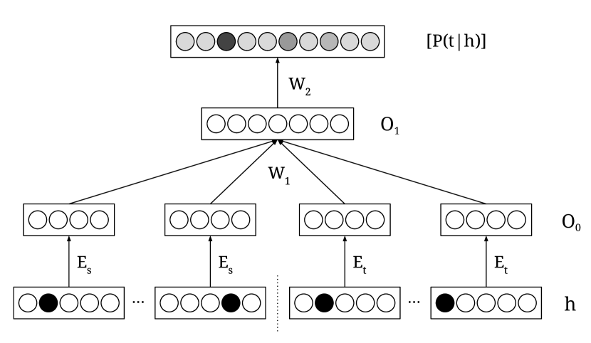
Figure 2: A single hidden layer neural network joint model

5.1 Model

The probability of the target hypothesis $T$ given the source sentence $S$ is estimated by the following equation:

$$P(T|S)\approx\prod_{i=1}^{|T|}P(t_{i}|h_{i})$$ (5)

where $|T|$ is the number of words in the target sentence, $t_{i}$ is the $i$^th target word, and $h_{i}$ is the context (history) for the target word $t_{i}$. The context $h_{i}$ consists of a set of $m$ source words represented by $(s_{a_{i}-\frac{m-1}{2}},\cdots,s_{a_{i}+\frac{m-1}{2}})$ and $n-1$ words preceding $t_{i}$ from the target sentence represented by $(t_{i-n+1},\cdots,t_{i-1})$. The context words from the source side are the words in the window of size $m$ surrounding the source word $s_{a_{i}}$ that is aligned to the target word $t_{i}$. The output of the neural network $P(t_{i}|h_{i})$ is the output of the final softmax layer which is given by the following equation:

$$P(t_{i}|h_{i})=\dfrac{1}{Z(h_{i})}\exp U_{i}(h_{i})$$ (6)

where $U_{i}(h_{i})$ is the output of the neural network before applying softmax and $Z(h_{i})$ is given by following equation:

$$Z(h_{i})=\sum_{i^{{}^{\prime}}=1}^{|V_{o}|}\exp U_{i^{{}^{\prime}}}(h_{i})$$

The output of the neural network before softmax is computed by applying output layer weights $W_{2}$ and biases $b_{2}$ to the hidden layer output $O_{1}$.

$$U(h_{i})=W_{2}\cdot O_{1}+b_{2}$$

$O_{1}$ is computed by applying weights $W_{1}$ and biases $b_{1}$ on the hidden layer input $O_{0}$ and using a non-linear activation function $\phi$:

$$O_{1}=\phi(W_{1}\cdot O_{0}+b_{1})$$

The input to the hidden layer ($O_{0}$) is a concatenated vector of context word embeddings:

$$O_{0}=( E_{s}\cdot\hat{s}_{a_{i}-\frac{m-1}{2}},\cdots,E_{s}\cdot\hat{s}_{a_{i}+\frac{m-1}{2}},$$

$$E_{t}\cdot\hat{t}_{i-n+1},\cdots,E_{t}\cdot\hat{t}_{i-1})$$

where $\hat{s}$ and $\hat{t}$ are the one-hot representations of the source word $s$ and the target word $t$, respectively. Similarly, $E_{s}$ and $E_{t}$ are the word embeddings matrices for the source words and the target words.

As we use log probabilities instead of raw probabilities in our GEC system, Equation 5 can be rewritten as the following:

$$\log P(t_{i}|h_{i})=U_{i}(h_{i})-\log Z(h_{i})$$ (7)

Finally, since the network is trained by Noise Contrastive Estimation (NCE) (described in Section 5.2), it becomes self-normalized. This means that $Z(h_{i})$ will be approximately 1 and hence the raw output of the neural network $U_{i}$ can be directly used as the log probabilities during decoding.

5.2 Training

To avoid the costly softmax layer and thereby speed up both training and decoding, we use Noise Contrastive Estimation (NCE) following Vaswani et al. (2013). During training, the negative log likelihood cost function is modified to a probabilistic binary classifier, which learns to discriminate between the actual target word and $k$ random words (noisy samples) per training instance selected from a noise distribution $q$. The two classes are $C=1$ indicating that the word is the target word and $C=0$ indicating that the word is a noisy sample. The conditional probabilities for $C=0$ and $C=1$ given a target word and context is given by:

$$P(C=1|t_{i},h_{i})=\dfrac{\tfrac{1}{k+1}P(t_{i}|h_{i})}{\tfrac{1}{k+1}P(t_{i}|h_{i})+\tfrac{k}{k+1}q(t_{i})}$$

$$P(C=0|t_{i},h_{i})=\dfrac{\tfrac{k}{k+1}q(t_{i})}{\tfrac{1}{k+1}P(t_{i}|h_{i})+\tfrac{k}{k+1}q(t_{i})}$$

where, $P(t_{i}|h_{i})$ is the model probability given in Equation 6. The negative log likelihood cost function is replaced by the following function.

$$L=-\sum_{i}\left[\log P(C=1|t_{i},h_{i})+\sum_{j=1}^{k}\log P(C=0|\bar{t}_{ij},h_{i})\right]$$

where $\bar{t}_{ij}$ refers to the $j$^th noise sample for the target word $t_{i}$. $Z(h_{i})$ is required for the computation of the neural network output, $P(t_{i}|h_{i})$. However, setting the term $Z(h_{i})$ to 1 during training forces the output of the neural network to be self-normalized. Hence, Equation 7 reduces to:

$$\log P(t_{i}|h_{i})\approx U_{i}(h_{i})$$ (8)

Using Equation 8 avoids the expensive softmax computation in the final layer and consequently speeds up decoding.

6 Experiments

We describe our experimental setup including the description of the data we used, the configuration of our baseline system and the neural network components, and the evaluation method in Section 6.1, followed by the results and discussion in Section 6.2

6.1 Setup

We use the popular phrase-based machine translation toolkit Moses as our baseline SMT system. NUCLE Dahlmeier et al. (2013), which is the official training data for the CoNLL 2013 and 2014 shared tasks, is used as the parallel text for training. Additionally, we obtain parallel corpora from Lang-8 Corpus of Learner English v1.0 Mizumoto et al. (2011), which consists of texts written by ESL (English as Second Language) learners on the language learning platform Lang-8. We use the test data for the CoNLL 2013 shared task as our development data. The statistics of the training and development data are given in Table 1. Source side refers to the original text written by the ESL learners and target side refers to the corresponding corrected text hand-corrected by humans. The source side and the target side are sentence-aligned and tokenized.

Dataset	No. of sentences	No. of source side tokens	No. of target side tokens
NUCLE	57,151	1,161,567	1,155,559
Lang-8 v1.0	1,114,139	12,945,666	13,232,058
CoNLL 2013	1,381	29,207	28,743

Table 1: Statistics of training and development data

We train the translation model for our SMT system using a concatenation of NUCLE and Lang-8 v1.0 parallel data. The training data is cleaned up by removing sentence pairs in which either the source or the target sentence is empty, or is too long (greater than 80 tokens), or violate a 9:1 sentence ratio limit. The translation model uses the default features in Moses which include the forward and inverse phrase translation probabilities, forward and inverse lexical weights, word penalty, and phrase penalty. We compute the phrase alignments using standard tools in Moses. We use two language model features: a 5-gram language model trained using the target side of NUCLE used for training the translation model and a 5-gram language model trained using English Wikipedia ($\sim$1.78 billion tokens). Both language models are estimated with KenLM using modified Kneser-Ney smoothing. We use MERT for tuning the feature weights by optimizing the $F_{0.5}$ measure (which weights precision twice as much as recall). This system constitutes our baseline system in Table 2. Our baseline system uses exactly the same training data as Susanto et al. (2014) for training the translation model and the language model. The difference between our baseline system and the SMT components of Susanto et al. (2014) is that we tune with $F_{0.5}$ instead of BLEU and we use the standard Moses configuration without the Levenshtein distance feature.

On top of our baseline system described above, we incorporate the two neural network components, neural network global lexicon model (NNGLM) and neural network joint model (NNJM) as features. Both NNGLM and NNJM are trained using the parallel data used to train the translation model of our baseline system.

We implement NNGLM using the Theano library in Python in order to make use of parallelization with GPUs, thus speeding up training significantly. We use a source and target vocabulary of 10,000 most frequent words on both sides. We use a single hidden layer neural network with 2,000 hidden nodes. We use $\tanh$ as the activation function for the hidden layer. We optimize the model weights by stochastic gradient descent using a mini-batch size of 100 and a learning rate of 10. We train the model for 45 epochs. The logistic regression function for rescaling is trained using the probabilities obtained from this model on the development set. To speed up tuning and decoding, we pre-compute the probabilities of target words using the source side sentences of the development and the test sets, respectively. We implement a feature function in Moses to compute the probability of a target hypothesis given the source sentence using the pre-computed probabilities.

To train NNJM, we use the publicly available implementation, Neural Probabilistic Language Model (NPLM) Vaswani et al. (2013). The latest version of Moses can incorporate NNJM trained using NPLM as a feature while decoding. Similar to NNGLM, we use the parallel text used for training the translation model in order to train NNJM. We use a source context window size of 5 and a target context window size of 4. We select a source context vocabulary of 16,000 most frequent words from the source side. The target context vocabulary and output vocabulary is set to the 32,000 most frequent words. We use a single hidden layer to speed up training and decoding with an input embedding dimension of 192 and 512 hidden layer nodes. We use rectified linear units (ReLU) as the activation function. We train NNJM with noise contrastive estimation with 100 noise samples per training instance, which are obtained from a unigram distribution. The neural network is trained for 30 epochs using stochastic gradient descent optimization with a mini-batch size of 128 and learning rate of 0.1.

We conduct experiments by incorporating NNGLM and NNJM both independently and jointly into our baseline system. The results of our experiments are described in Section 6.2. The evaluation is performed similar to the CoNLL 2014 shared task setting using the the official test data of the CoNLL 2014 shared task with annotations from two annotators (without considering alternative annotations suggested by the participating teams). The test dataset consists of 1,312 error-annotated sentences with 30,144 tokens on the source side. We make use of the official scorer for the shared task, M²Scorer v3.2 Dahlmeier and Ng (2012), for evaluation. We perform statistical significance test using one-tailed sign test with bootstrap resampling on 100 samples.

6.2 Results and Discussion

Table 2 presents the results of our experiments with neural network global lexicon model (NNGLM) and neural network joint model (NNJM).

System	P	R	F0.5
Baseline	50.56	22.68	40.58
Baseline + NNGLM	50.73	23.21	41.01*
Baseline + NNJM	51.39	23.26	41.38*
Baseline + NNGLM + NNJM	52.34	23.07	41.75*

Table 2: Results of our experiments with NNGLM and NNJM on the CoNLL 2014 test set (^* indicates statistical significance with $p<0.01$)

We see that the addition of both NNGLM and NNJM to our baseline individually improves $F_{0.5}$ measure on the CoNLL 2014 test set by 0.43 and 0.80, respectively. Although both improvements over the baseline are statistically significant (with $p<0.01$), we observe that the improvement of NNGLM is slightly lower than that of NNJM. NNGLM encodes the entire lexical information from the source sentence without word ordering information. Hence, it focuses mostly on the choice of words appearing in the output. Many of the words in the source context may not be necessary for ensuring the quality of corrected output. On the other hand, NNJM looks at a smaller window of words in the source side. NNJM can act as a language model and can ensure a fluent translation output compared to NNGLM.

We also found rescaling to be important for NNGLM because of imbalanced training data. While the most frequent words in the data, ‘I’ and to’, appear in 43% and 27% of the training sentences, respectively, most words occur in very few sentences only. For example, the word ‘set’ appears in 0.15% of the sentences and the word ‘enterprise’ appears in 0.003% of the sentences.

System: Baseline + NNGLM
Source	However , there are also a great amount of people who against this technology .
Baseline	However , there are also a great amount of people who are against this technology .
System	However , there are also a great number of people who are against this technology .
Reference	However , there are also a great number of people who are against this technology .
System: Baseline + NNJM
Source	The parents give knowledge and love to the children , meanwhile they feel happy with the accompany of the children .
Baseline	The parents give knowledge and love to the children , while they feel happy with the accompaniment of the children .
System	The parents give knowledge and love to the children , meanwhile they feel happy with the company of the children .
Reference	The parents give knowledge and love to the children , meanwhile they feel happy with the company of the children .
System: Baseline + NNGLM + NNJM
Source	… by equipping them with a powerful tool to disseminate information almost immediate to the people around them .
Baseline	… by equipping them with a powerful tool to disseminate information almost immediate to the people around them .
System	… by equipping them with a powerful tool to disseminate information almost immediately to the people around them .
Reference	… by equipping them with a powerful tool to disseminate information almost immediately to the people around them .

Table 3: Examples from the outputs of the systems compared against our baseline system. ‘Source’ is the erroneous input sentence, ‘Baseline’ and ‘System’ are the outputs of our baseline and our neural networks-enhanced system, respectively. ‘Reference’ is the corrected sentence in which the corrections are made by a human annotator.

By incorporating both components together, we obtain an improvement of 1.17 in terms of $F_{0.5}$ measure. This indicates that both components are beneficial and complement each other to improve the performance of the baseline system. While NNGLM looks at the entire source sentence and ensures the appropriate choice of words to appear in the output sentence, NNJM encourages the system to choose appropriate corrections that give a fluent output.

We compare our system to the top 3 systems in the CoNLL 2014 shared task and to the best published results Yuan and Briscoe (2016); Susanto et al. (2014) on the test data of the CoNLL 2014 shared task. The results are summarized in Table 4. Our final system including both neural network models outperforms the best system Yuan and Briscoe (2016) by 1.85 in F_0.5 measure. It should be noted that this is despite the fact that the system proposed in Yuan and Briscoe (2016) uses much larger training data than our system.

System	P	R	F0.5
Baseline + NNGLM + NNJM	52.34	23.07	41.75
Baseline	50.56	22.68	40.58
Yuan and Briscoe (2016)	-	-	39.90
Susanto et al. (2014)	53.55	19.14	39.39
Top 3 systems in the CoNLL 2014 shared task
CAMB	39.71	30.10	37.33
CUUI	41.78	24.88	36.79
AMU	41.62	21.40	35.01

Table 4: Our system compared against competitive grammatical error correction systems. CAMB, CUUI, and AMU are Team IDs in the CoNLL 2014 shared task.

We qualitatively analyze the output of our neural network-enhanced systems against the outputs produced by our baseline system. We have included some examples in Table 3 and the corresponding outputs of the baseline system and the reference sentences. The selected examples show that NNGLM and NNJM choose appropriate words by making use of the surrounding context effectively.

Note that our neural networks, which rely on fixed source and target vocabulary, map the rare words and misspelled words to the UNK token. Therefore, phrases with the UNK token may get a higher probability than they actually should due to the large number of UNK tokens seen during training. This leads to fewer spelling error corrections compared to the baseline system which does not employ these neural networks. Consider the following example from the test data:
… numerous profit-driven companies realize the hugh (huge) human traffic on such social media sites ….
The spelling error hugh $\rightarrow$ huge is corrected by the baseline system, but not by our final system with the neural networks. This is because the misspelled word hugh is not in the neural network vocabulary and so it is mapped to the UNK token. The sentence with the UNK token gets a higher score and hence the system chooses this output over the correct one.

From our experiments and analysis, we see that NNGLM and NNJM capture contextual information better than regular translation models and language models. This is because they make use of larger source sentence contexts and continuous space representation of words. This enables them to make better predictions compared to traditional translation models and language models. We also observed that our system has an edge over the baseline for correction of word choice and collocation errors.

7 Conclusion

Our experiments show that using the two neural network translation models improves the performance of a phrase-based SMT approach to GEC. To the best of our knowledge, this is the first work that uses these two neural network models for SMT-based GEC. The ability of neural networks to model words and phrases in continuous space and capture non-linear relationships enables them to generalize better and make more accurate grammatical error correction. We have achieved state-of-the-art results on the CoNLL 2014 shared task test dataset. This has been done without using any additional training data compared to the best performing systems evaluated on the same dataset.

References

- Bengio et al. [2003] Yoshua Bengio, Réjean Ducharme, Pascal Vincent, and Christian Janvin. A neural probabilistic language model. Journal of Machine Learning Research, 3:1137–1155, 2003.
- Brockett et al. [2006] Chris Brockett, William B. Dolan, and Michael Gamon. Correcting ESL errors using phrasal SMT techniques. In Proc. of ACL, 2006.
- Dahlmeier and Ng [2012] Daniel Dahlmeier and Hwee Tou Ng. Better evaluation for grammatical error correction. In Proc. of NAACL, 2012.
- Dahlmeier et al. [2012] Daniel Dahlmeier, Hwee Tou Ng, and Eric Jun Feng Ng. NUS at the HOO 2012 shared task. In Proceedings of the Seventh Workshop on Building Educational Applications Using NLP, 2012.
- Dahlmeier et al. [2013] Daniel Dahlmeier, Hwee Tou Ng, and Siew Mei Wu. Building a large annotated corpus of learner English: The NUS corpus of learner English. In Proceedings of the Eighth Workshop on Innovative Use of NLP for Building Educational Applications, 2013.
- Dale and Kilgarriff [2011] Robert Dale and Adam Kilgarriff. Helping Our Own: The HOO 2011 pilot shared task. In Proceedings of the 13th European Workshop on Natural Language Generation, 2011.
- Dale et al. [2012] Robert Dale, Ilya Anisimoff, and George Narroway. HOO 2012: A report on the preposition and determiner error correction shared task. In Proceedings of the Seventh Workshop on Building Educational Applications Using NLP, 2012.
- Devlin et al. [2014] Jacob Devlin, Rabih Zbib, Zhongqiang Huang, Thomas Lamar, Richard Schwartz, and John Makhoul. Fast and robust neural network joint models for statistical machine translation. In Proc. of ACL, 2014.
- Felice et al. [2014] Mariano Felice, Zheng Yuan, Øistein E. Andersen, Helen Yannakoudakis, and Ekaterina Kochmar. Grammatical error correction using hybrid systems and type filtering. In Proc. of CoNLL Shared Task, 2014.
- Ha et al. [2014] Thanh-Le Ha, Jan Niehues, and Alex Waibel. Lexical translation model using a deep neural network architecture. In Proceedings of the 11th International Workshop on Spoken Language Translation, 2014.
- Junczys-Dowmunt and Grundkiewicz [2014] Marcin Junczys-Dowmunt and Roman Grundkiewicz. The AMU system in the CoNLL-2014 shared task: Grammatical error correction by data-intensive and feature-rich statistical machine translation. In Proc. of CoNLL Shared Task, 2014.
- Koehn et al. [2003] Philipp Koehn, Franz Josef Och, and Daniel Marcu. Statistical phrase-based translation. In Proc. of NAACL, 2003.
- Mauser et al. [2009] Arne Mauser, Saša Hasan, and Hermann Ney. Extending statistical machine translation with discriminative and trigger-based lexicon models. In Proc. of EMNLP, 2009.
- Mizumoto et al. [2011] Tomoya Mizumoto, Mamoru Komachi, Masaaki Nagata, and Yuji Matsumoto. Mining revision log of language learning SNS for automated Japanese error correction of second language learners. In Proc. of IJCNLP, 2011.
- Ng et al. [2013] Hwee Tou Ng, Siew Mei Wu, Yuanbin Wu, Christian Hadiwinoto, and Joel Tetreault. The CoNLL-2013 shared task on grammatical error correction. In Proc. of CoNLL Shared Task, 2013.
- Ng et al. [2014] Hwee Tou Ng, Siew Mei Wu, Ted Briscoe, Christian Hadiwinoto, Raymond Hendy Susanto, and Christopher Bryant. The CoNLL-2014 shared task on grammatical error correction. In Proc. of CoNLL Shared Task, 2014.
- Rozovskaya et al. [2014] Alla Rozovskaya, Kai-Wei Chang, Mark Sammons, Dan Roth, and Nizar Habash. The Illinois-Columbia system in the CoNLL-2014 shared task. In Proc. of CoNLL Shared Task, 2014.
- Sun et al. [2015] Chengjie Sun, Xiaoqiang Jin, Lei Lin, Yuming Zhao, and Xiaolong Wang. Convolutional neural networks for correcting English article errors. In Proceedings of the 4th CCF Conference on Natural Language Processing and Chinese Computing, 2015.
- Susanto et al. [2014] Raymond Hendy Susanto, Peter Phandi, and Hwee Tou Ng. System combination for grammatical error correction. In Proc. of EMNLP, 2014.
- Vaswani et al. [2013] Ashish Vaswani, Yinggong Zhao, Victoria Fossum, and David Chiang. Decoding with large-scale neural language models improves translation. In Proc. of EMNLP, 2013.
- Wu et al. [2014] Jian-Cheng Wu, Tzu-Hsi Yen, Jim Chang, Guan-Cheng Huang, Jimmy Chang, Hsiang-Ling Hsu, Yu-Wei Chang, and Jason S. Chang. NTHU at the CoNLL-2014 shared task. In Proc. of CoNLL Shared Task, 2014.
- Yuan and Briscoe [2016] Zheng Yuan and Ted Briscoe. Grammatical error correction using neural machine translation. In Proc. of NAACL, 2016.