Solvable Chaotic Synchronization
–A New Interpretation of Common Noise-induced Synchronization
with Conditional Lyapunov Exponents–

Abstract

We present a solvable chaotic synchronization model of unidirectionally coupled dynamical systems. We establish a new interpretation of the conditional Lyapunov exponent that characterizes chaotic synchronization completely. Moreover, we newly show how the conditional Lyapunov exponent relates to common noise-induced synchronization phenomena by the new interpretation.

Chaotic signal induced synchronization so called chaotic synchronization is known to occur robustly in various physical models Fujisaka_Yamada_1983 ; Peroca_Carroll_1990 ; Kocarev_Parlitz_1995 ; Kocarev_Parlitz_1996 ; Fujisaka_1997 . The conditional Lyapunov exponents (CLEs) are used for detecting chaotic synchronization and these play an important role in an indication of chaotic synchronization. However, most previous studies on chaotic synchronization obtains CLEs numerically, and none of the studies have proven chaotic synchronization for a given model except the numerical simulations while chaotic synchronizaton have been experimentally observed sunada2014 ; umeno_2005 . In this Letter, we show an analytically solvable model of chaotic synchronization where the CLEs are exactly obtained in terms of the coupling strength by the ergodicity of solvable chaos umeno_1998 ; umeno_1997 used in our model. In addition, a new genaral relation of CLE is established, which provide a new interpretation of a common noise-induced synchronization mechanism Teramae_Tanaka_2004 .
Here, we consider a class of dynamical systems with a chaotic map $f$ as follows

$$\begin{cases}X_{n+1}&=f(X_{n})\\ Y_{n+1}&=f(Y_{n})+\varepsilon X_{n}\equiv g_{\varepsilon}(X_{n},Y_{n}).\end{cases}$$ (1)

The dynamical system (1) can be a model for unidirectionally coupled system. Here, the system $f$ shows chaotic behavior while $\varepsilon$ represents the strength of coupling connection.
We choose $f$ as a solvable chaotic map umeno_1998 as follows

$$X_{n+1}=\frac{1}{2}\left(X_{n}-\frac{1}{X_{n}}\right)\equiv f(X_{n}).$$ (2)

The function $f$ is one of the generalized Boolean transformations, and is based on the duplication fomula of a cotangent function. In addition, the function $f$ satisfies $-\cot{2\theta}=f[-\cot{\theta}]$ umeno_1998 ，and $X_{n}$ has an analytically solvable solution $X_{n}=-\cot((\pi/2)2^{n}\theta_{0})$ with $X_{0}$ being an initial point. The mapping $f$ is a two-to-one mapping, and the ergodic invariant measure $\mu({\rm d}x)=\rho(x){\rm d}x$ of dynamical system (2) satisfies the probability preservation relation (The Perron-Frobenius equation  [PF equation]), given by

$$\rho(z)=\sum_{x=f^{-1}(z)}\rho(x)\left|\frac{{\rm d}x}{{\rm d}z}\right|.$$

We note that the standard Cauchy distribution, satisfying the PF equationumeno_1998 , and which shows that $f$ preserves the standard Cauchy Law.

$$\rho(x){\rm d}x=\frac{1}{\pi(x^{2}+1)}{\rm d}x\hskip 8.53581pt(\equiv{\rm C}(x;0,1){\rm d}x)$$

In addition, the Lyapunov exponent of the dynamical system (2) is analytically calculated by using the invariant measure, by the ergodic equality.

$$\lambda_{f} = \lim_{N\to\infty}\frac{1}{N}\sum_{n=0}^{N-1}\log\left|\frac{{\rm d}f(x)}{{\rm d}x}\right|_{x=X_{n}}$$

$$= \int_{\mathbb{R}}\frac{1}{\pi(x^{2}+1)}\log\left|\frac{1}{2}\left(1+\frac{1}{x^{2}}\right)\right|{\rm d}x=\log{2}$$

Here, we say that a chaotic system is solvable if the ergodic invariant measure of dynamical system can be analytically obtained. We define a chaotic synchronization as follows. When we give the same initial points $X_{0}$ and the different initial points $Y_{0}$ and $Y^{\prime}_{0}$ in two unieque dynamical systems, a chaotic synchronization occurs for unidirectionally coupled dynamical systems (1) if the condition (3) is satisfied for any $Y_{0}\neq Y^{\prime}_{0}$ almost everywhere.

$$\lim_{n\to\infty}|Y_{n}-Y^{\prime}_{n}|=0\ \ \text{a.e.}$$ (3)

The CLE is an index of indicating whether chaotic synchronization actually occur or not. Given the variations in the mapping for variables $X_{n}$ and $Y_{n}$ in the dynamical system (1), we have the following variational equations for considering the sensitive dependency with respect to the initial conditions. Here, $J_{k}$ is the Jacobian matrix satisfying the following linear relation.

$$\left(\begin{array}[]{@{\,}c@{\,}}\delta X_{n}\\ \delta Y_{n}\end{array}\right)=\prod_{k=1}^{n}J_{k}\left(\begin{array}[]{@{\,}c@{\,}}\delta X_{0}\\ \delta Y_{0}\end{array}\right)$$ (8)

When we define a matrix $A_{n}$ as $\prod_{k=1}^{n}J_{k}=J_{n}J_{n-1}\dots J_{1}$, we can describe $A_{n}$ as follows.

$$A_{n} =\left(\begin{array}[]{@{\,}cc@{\,}}\displaystyle\prod_{k=1}^{n}\frac{\partial f(x)}{\partial x}\Biggl{|}_{x=X_{k-1}}\Biggr{.}&0\\ \dots&\displaystyle\prod_{k=1}^{n}\frac{\partial g_{\varepsilon}(x,y)}{\partial y}\Biggl{|}_{\scriptsize{\begin{matrix}x=X_{k-1},\\ y=Y_{k-1}\end{matrix}}}\Biggr{.}\end{array}\right)$$

Here, the limiting behaviour of the component (1,1) of $A_{n}$ has been found to be $2^{n}$ as $n\to\infty$ since the Lyapunov exponent of the system (2) is $\log 2$. On the other hand, the CLE for variable $y$ in the dynamical system (1) can be determined by the limiting behaviour of the component (2,2) of $A_{n}$. In addition, we will show later that the CLE $\lambda_{y}$ in the dynamical system (1) with the mapping (2) is analytically obtained in terms of the coupling strength $\varepsilon$ by the ergodicity of the following long time average formula:

$$\displaystyle\lambda_{y} =\lim_{n\to\infty}\frac{1}{n}\log\prod_{k=1}^{n}\left|\frac{\partial g_{\varepsilon}(x,y)}{\partial y}\right|_{x=X_{k-1},y=Y_{k-1}}$$

$$=\lim_{n\to\infty}\frac{1}{n}\sum_{k=1}^{n}\log\left|\frac{\partial g_{\varepsilon}(x,y)}{\partial y}\right|_{x=X_{k-1},y=Y_{k-1}}.$$ (10)

When CLE for the variable $y$ is negative, it can be seen from (8) that the chaotic synchronization actually occur satisfying (3). Note that generally their CLEs are obtained by numerical calculation (long-term average) according to the definition (10) except our solvable case. According to the previous studies umeno_1998 ; umeno_okubo_2016 , it is proved that the dynamical system (2) has ergodicity and the mixing property. We consider the invariant measure of the coupled dynamical system (1) with the solvable chaotic mapping (2) in order to show that this system is solvable. Since the probability distribution of the variable $x$ is already known to be the standard ${\rm Cauchy}$ distribution, it is necessary to show that the probability distribution of the variable $y$ converges to a certain probability distribution $P_{\varepsilon}(y)$ analytically. In order to show them, we consider the PF equation for the coupling relation (1) with the mapping $f$ again and the nature of the stable distribution in the superposition of Cauchy distributions.
At first, we consider the PF equation for the equation $z=f(x)$ where input variables $x$ follow a Cauchy distribution ${\rm C}(x;0,\gamma)$ with a scale parameter $\gamma$. Here, C means that ${\rm C}(x;0,\gamma)=\frac{\gamma}{\pi(x^{2}+\gamma^{2})}$. Since the $f$ is a two-to-one mapping, $P(z)$ satisfies Pf equation:

$$P(z)|{\rm d}z|=P(x_{1})|{\rm d}x_{1}|+P(x_{2})|{\rm d}x_{2}|,$$ (11)

where $x_{1}$ and $x_{2}$ $(x_{1}>x_{2})$ are the solutions of the quadratic equation $z=f(x)$. They satisfy the following formula,:

$$\begin{cases}x_{1}+x_{2}=2z\\ x_{1}x_{2}=-1.\\ \end{cases}$$

Considering these relationships, the probability distribution $P(z)$ is obtained, as the following rescaled Cauchy distribution:

$$P(z)={\rm C}(z;0,\gamma^{\prime})\ \left(\gamma^{\prime}=\frac{\gamma^{2}+1}{2\gamma}\ \text{\cite[cite]{\@@bibref{Authors Phrase1YearPhrase2}{shintani_2015,umeno_2016}{\@@citephrase{(}}{\@@citephrase{)}}}}\right).$$ (12)

Thus, we can show that the mapping $f$ preserves Cauchy distributions with a change of the scale parameter as $\gamma\to\gamma^{\prime}\$for any scale parameters $\gamma$. Considering the invariance property of Cauchy distributions, and the superposition of Cauchy distributions,we get the recurrence equation shintani_2015 about the scale parameter $\gamma_{n}$ of the Cauchy distributions for $Y_{n}$ of (1).

$$\gamma_{n+1}=\frac{\gamma_{n}^{2}+1}{2\gamma_{n}}+|\varepsilon|$$ (13)

From this self-consistent recurrence equation in (13), the scale parameter converges to the fixed point of (13) $\gamma^{*}(=|\varepsilon|+\sqrt{\varepsilon^{2}+1}(\geq 1))$. Thus, $P(y)$ converges to the probability distribution ${\rm C}(y:0,\gamma^{*})$. Thus far, though we can set an initial distribution as a Cauchy distribution with any scale parameter $\gamma(>0)$, these relations are satisfied for almost all the initial distributions because the basis dynamical system (2) has mixing property. As above $P_{\varepsilon}(y)$ is expressed analytically, and we finally get the formula (14).

$$P_{\varepsilon}(y)={\rm C}(y;0,\gamma^{*})\ \left(\gamma^{*}=|\varepsilon|+\sqrt{\varepsilon^{2}+1}\right)$$ (14)

Secondly, because the probability distribution $P_{\varepsilon}(y)$ is obtained, the CLE in (10) can be expressed as a phase average by the ergodic theorem:

$$\lambda_{y}=\int_{\mathbb{R}}\frac{\gamma^{*}}{\pi(y^{2}+{\gamma^{*}}^{2})}\log\left|\frac{1}{2}\left(1+\frac{1}{y^{2}}\right)\right|{\rm d}y.$$

This integration can be calculated analytically, and we get the analytical CLE in terms of the strength of connection $\varepsilon$ as

$$\begin{split}\lambda_{y}(\varepsilon)&=2\log\left(\frac{\gamma^{*}+1}{\gamma^{*}}\right)-\log{2}\\ &=2\log{(\sqrt{\varepsilon^{2}+1}-|\varepsilon|+1)}-\log{2}.\end{split}$$ (15)

Then the threshold of synchronization $\varepsilon_{c}$ can also be obtained by the solution of $\lambda_{y}(\varepsilon)=0$. In the dynamical system (1), two different initial conditions $Y_{0}$ and $Y_{0}^{\prime}$ synchronize if and only if the following condition is satisfied.

$$\lim_{n\to\infty}|Y_{n}-Y^{\prime}_{n}|=0\hskip 11.38109pt\Leftrightarrow\hskip 11.38109pt|\varepsilon|>\varepsilon_{c},\\$$

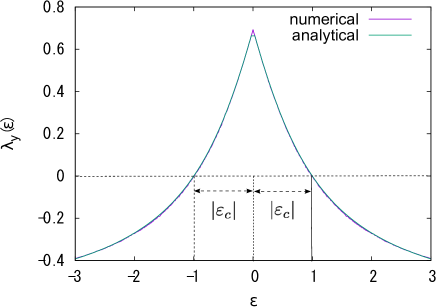
where $\varepsilon_{c}$ satisfies $\lambda_{y}(\varepsilon_{c})=0$, giving the critical coupling strength as $\varepsilon_{c}=1$. FIG. 1 illustrates that this analytical CLE exactly corresponds to the numerically obtained CLE by the fomula in (10).

Figure 1: Conditional Lyapunov exponent $\lambda_{y}(\varepsilon)$

As above, we show that the dynamical system (1) is solvable when $f(x)$ is given by a solvable chaos mapping in (2) with the stable Cauchy law as an ergodic invariant measure, and derive the CLE and the threshold of chaotic synchronization analytically. Furthermore, we can also get the CLE and the threshold for another dynamical system (1) analytically. For example, we use another solvable chaos mapping $f$ as $\displaystyle X_{n+1}=2X_{n}/\left(X_{n}^{2}-1\right)$ umeno_1998 with the standard Cauchy law as the ergodic invariant measure, which is based on the doubling formula of a tangent function, and consider the same unidirectional coupled system in (1). In this case, we get the following probability distribution $P_{\varepsilon}(y)$, the CLE $\lambda_{y}(\varepsilon)$ and the threshold $\varepsilon_{c}$ satisfying $\lambda_{y}(\varepsilon)=0$ respectively:

$$P_{\varepsilon}(y)={\rm C}(y;0,\gamma^{*})$$

with $\gamma^{*}$ satisfying ${\gamma^{*}}^{2}-|\varepsilon|{\gamma^{*}}^{2}-\gamma^{*}-|\varepsilon|=0$, and

$$\lambda_{y}(\varepsilon) = \int_{\mathbb{R}}\frac{\gamma^{*}}{\pi(y^{2}+{\gamma^{*}}^{2})}\log\left|\frac{2(1+y^{2})}{(1-y^{2})^{2}}\right|{\rm d}y$$

$$= 2\log\left(\frac{\gamma^{*}+1}{{\gamma^{*}}^{2}+1}\right)+\log{2},$$

and $\lim_{n\to\infty}|Y_{n}-Y^{\prime}_{n}|=0\ \ \text{for}\ \ |\varepsilon|>\varepsilon_{c}$, where $\varepsilon_{c}$ satisfies $\lambda_{y}(\varepsilon_{c})=0$, giving the correspoding critical coupling strength as $\varepsilon_{c}=0.78\cdots$.
Two series with different initial conditions $Y_{0}$ and $Y_{0}^{\prime}$ synchronize if and only if the coupling strength satisfies $|\varepsilon|>\varepsilon_{c}$. Note that this critical coupling strength $\varepsilon_{c}$ is different from that of the former case that $f$ is given by (2).
Next, we explain how the CLE relates to the coupling strength in a genaral framework of common noise-induced synchronization. The CLE can be considered one of the dynamical values ​​obtained as a result from two-dimensional dynamical systems (1), meaning an orbital expansion rate according to a change of a dynamical variable. Here, we decompose the analysis of the dynamical system (1) into the following two stages. We consider changes of the induced (skew-product) mapping at first, and then averege out these each orbital expansion rate. We define the induced mapping $G_{x}(y)$ as follows:

$$G_{x}(y)=f(y)+x.$$

Here, the Lyapunov exponent of this mapping $G_{x}(y)$ depends on the input value $x$ and consider as a skew product transformation. We analytically calculate the Lyapunov exponent of $G_{x}(y)$ for each value $x$ by considering the distributions of $y$. Note the probabirity distribution of $y$ can be considered as a conditional probability $P(y|x)$ because $y$ depends on the value $x$. Then, the method of deriving $P(y|x)$ is again from the probability preservation relation as we obtain $P(y)$ in Eqs.(11)-(14). Assume that input variables $y$ of $f$ that follow a Cauchy distribution ${\rm C}(y;c,\gamma)$. Then $P(z)$ is given by considering the PF equation for $z=f(y)$, as

$$\begin{split}&P(z)=\frac{\gamma^{\prime}}{\pi\left\{(z-c^{\prime})^{2}+\gamma^{\prime 2}\right\}}\hskip 8.53581pt=\ \ {\rm C}(z;c^{\prime},\gamma^{\prime}),\\ &\text{where}\ \gamma^{\prime}=\frac{\gamma(\gamma^{2}+c^{2}+1)}{2(\gamma^{2}+c^{2})},\text{and}\hskip 5.69054ptc^{\prime}=\frac{c(\gamma^{2}+c^{2}-1)}{2(\gamma^{2}+c^{2})}.\end{split}$$ (16)

This expression of $P(z)$ is more general than (12) because it has a change of the median as $c\to c^{\prime}$. When we consider the superpositon of distributions $f(y)+x$, we can regard the constant value distribution $x$ in the mapping $G_{x}(y)$ as the delta funcion $\delta(x)$. Remark that the Delta function can be defined as a specific Cauchy distribution ${\rm C}(y;x,\eta)$ with the scale parameter $\eta$ $\to$ $0$. Considering the dynamical system in this way, it is sufficient to consider a distribution of $f(y)+x$ within the class of Cauchy distributions. We get the following self-consistent recurrence equations about a median $c$ and a scale parameter $\gamma$, as

$$\left\{\begin{split}c_{n+1}&=\frac{c_{n}(\gamma_{n}^{2}+c_{n}^{2}-1)}{2(\gamma_{n}^{2}+c_{n}^{2})}+x\\ \gamma_{n+1}&=\frac{\gamma_{n}(\gamma_{n}^{2}+c_{n}^{2}+1)}{2(\gamma_{n}^{2}+c_{n}^{2})}+\eta.\end{split}\right.$$ (17)

We get the convergence values $\hat{c}$ and $\hat{\gamma}$ as the stable fixed point of (17) for $\eta\to 0$, where

$$\begin{split}&\left\{\begin{split}\hat{c}&=x\\ \hat{\gamma}&=\sqrt{1-x^{2}}\end{split}\ \ \ \ \ \ \ (\text{if}\ |x|<1),\right.\\ &\left\{\begin{split}\hat{c}&=x+\text{sgn}(x)\sqrt{x^{2}-1}\\ \hat{\gamma}&=0\end{split}\ (\text{if}\ |x|\geq 1),\right.\end{split}$$

and $\text{sgn}(x)=\left\{\begin{matrix}1\ \ \text{if}\ x>0.\\ -1\ \text{if}\ x<0.\end{matrix}\right.$
Thus, we finally obtain the conditional probability distribution $P(y|x)$, as

$$P(y|x)=\left\{\begin{split}&{\rm C}(y;x,\sqrt{1-x^{2}})&(|x|<1).\\ &{\rm C}(y;x+{\rm sgn}(x)\sqrt{x^{2}-1}),0)&(|x|\geq 1).\end{split}\right.$$ (18)

Finally, we estimate the Lyapunov exponent $\lambda_{G}(x)$ as the phase average, and get it analytically by solving its integration, as

$$\lambda_{G}(x)=\Bigg{\langle}\log\left|\frac{{\rm d}G_{x}(y)}{{\rm d}y}\right|\Bigg{\rangle}_{P(y|x)}$$ (19)

$$= \int_{\mathbb{R}}P(y|x)\log{\left|\frac{1}{2}\left(1+\frac{1}{y^{2}}\right)\right|}{\rm d}y$$

$$= \begin{cases}\log(1+\sqrt{1-x^{2}})\ \ \ \ (|x|<1)\\ \log\left\{1+\frac{1}{(x+{\rm sgn}(x)\sqrt{x^{2}-1})^{2}}\right\}-\log 2\ (|x|\geq 1),\end{cases}$$

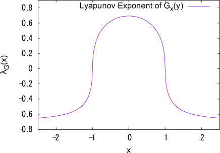
where $\langle\cdot\rangle$ represents the phase average. FIG. 2 illustrates the relation between $x$ and $\lambda_{G}(x)$.

Figure 2: the relation between $x$ and $\lambda_{G}(x)$

As can be seen from FIG. 2, the Lyapunov exponent of the dynamical system $G_{x}(Y_{n+1})=f(Y_{n})+x$ changes depending on the value $x$. Note that for $|x|>1$, the mapping $G_{x}(y)$ become no longer a chaotic map because of the negative Lyapunov exponent $\lambda_{G}(x)$, and the dynamical system has a unique stable point for almost all the initial points. Having $\lambda_{G}(x)$, then we calculate the weighted average of these Lyapunov exponents according to the distribution of $x$. Note that this value $x$ which is originally the variable $\varepsilon X_{n}$ that follow ${\rm C}(x;0,|\varepsilon|)$, as $\frac{|\varepsilon|}{\pi(x^{2}+\varepsilon^{2})}\equiv P_{\varepsilon}(x)$.
Thus we can calculate the averaged value that equals to $\lambda_{y}$. That is, the CLE can be given as the weighted averages of the Lyapunov exponents $\lambda_{G}(x)$, that can be considered a new relation for CLE.

$$\lambda_{y} = \Big{\langle}\lambda_{G}(x)\Big{\rangle}_{P(x)}$$ (20)

$$= \int_{\mathbb{R}}P_{\varepsilon}(x)\left(\int_{\mathbb{R}}P(y|x)\log\left|\frac{{\rm d}G_{x}(y)}{{\rm d}y}\right|{\rm d}y\right){\rm d}x$$

$$\bigl{(}\bigr{.} = 2\log{(\sqrt{\varepsilon^{2}+1}-|\varepsilon|+1)}-\log{2},\ \text{when}\ f\ \text{is}\ \text{\eqref{eq:f}}\bigl{.}\bigr{)}$$

FIG. 2 illustrates that the mapping $G_{x}(y)$ is expansive when $|x|<1$ while it is attractive when $|x|>1$. For $P_{\varepsilon}(x)(=P(\varepsilon X_{n}))$, the increase in $|\varepsilon|$ is equivalent to having an effect on widening the tails of the Cauchy distribution of the probability density function $P(x)$.
Thus, the increase in $|\varepsilon|$ increases the outer weights of $\lambda_{G}(x)$ in FIG. 2 when we calculate the CLE by the formula (20). Then, the CLE converts to negative when the weight of attractive mappings is relatively larger than the weight of expansive mappings. In this way, the coupling strength $\varepsilon$ relates to CLE and the origin of the common noise-induced synchronization. Now remark that the CLE does not depend on whether $x$ is deterministic chaotic or non-deterministic random noise, but purely depends on the distribution of $x$, namely $P_{\varepsilon}(x)=P(\varepsilon X_{n})$. In fact, even when using the equation $\displaystyle X_{n+1}=2X_{n}/\left(X_{n}^{2}-1\right)$ for the mapping $f$ with the same standard Cauchy distribution ${\rm C}(x;0,1)$, the CLE of the dynamical system (1) is confirmed to have the same expression in (20).
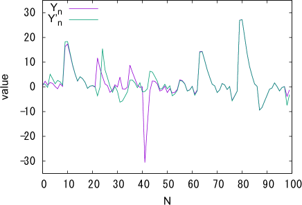
Since the CLE represents the phase average of the orbit expansion rate, temporal orbit expansion rate can not accurately represent the synchronization behavior of the dynamical system. In fact as shown in FIG. 3, we can confirm that an orbit expansion (de-synchronizaton) can temporarily appear, even when the CLE is negative. This fact can be understood from the fact that the effect of the noise amplitude of the mapping in the dynamical system affects a temporal synchronization behavior, such as previously described in FIG. 2.

Figure 3: An example of a chaotic synchronization

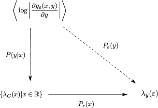
Finally, the background of the relation (20) is explained by the concept of marginalization of probability. Note that for the terms with the formula (10) and (20), the following relation is generally satisfied for unidirectional coupled dynamical systems (1).

$$\frac{\partial g_{\varepsilon}(x,y)}{\partial y}=\frac{{\rm d}G_{x}(y)}{{\rm d}y}=\frac{{\rm d}f(y)}{{\rm d}y}.$$

Forthemore, the probability $P(y)$ is expressed in terms of the maginal probability density function $P(y|x)$ as

$$P(y)=\int_{\mathbb{R}}P(x)P(y|x){\rm d}x$$

Thus, we obtain the relation (20) which gives a new interpretation of the common noise-induced synchronization. This relation can conceptually be depicted in FIG. 4 via the marginal probability formula as:

$$\lambda_{y}(\varepsilon) = \int_{\mathbb{R}}P_{\varepsilon}(y)\log\left|\frac{\partial g_{\varepsilon}(x,y)}{\partial y}\right|{\rm d}y$$

$$= \int_{\mathbb{R}}\left(\int_{\mathbb{R}}P_{\varepsilon}(x)P(y|x){\rm d}x\right)\log\left|\frac{{\rm d}f(y)}{{\rm d}y}\right|{\rm d}y$$

$$= \int_{\mathbb{R}}P_{\varepsilon}(x)\left(\int_{\mathbb{R}}P(y|x)\log\left|\frac{{\rm d}G_{x}(y)}{{\rm d}y}\right|{\rm d}y\right){\rm d}x$$

$$= \int_{\mathbb{R}}P_{\varepsilon}(x)\lambda_{G}(x){\rm d}x.$$

In conclusion, we have obtained a model of solvable chaotic synchronization, where we analytically have obtained the CLE, a threshold of chaos synchronization and an exact limiting distribution of the coupled the dynamical systems (1). Moreover, we also have obtained the new relation for the CLE by considering the local analytical Lyapunov exponents of the induced (skew-product) transformation, and have proven that a negative CLE causing the common noise-induced synchronization in unidirectional coupled two-dimensional chaotic dynamical systems have been consistent with the local Lyapunov exponent $\lambda_{G}(x)$, which could have had a positive value causing temporally expansive behabior.

Figure 4: the new relation for CLE

References

- (1) H. Fujisaka and T. Yamada, Prog. Theor. Phys. 69, 32 (1983)
- (2) L. M. Pecora and T. L. Carroll, Phys. Rev. Lett. 64, 821 (1990)
- (3) L. Kocarev and U. Parlitz, Phys. Rev. Lett. 74, 5028 (1995)
- (4) L. Kocarev and U. Parlitz, Phys. Rev. Lett. 76, 1816 (1996)
- (5) H. Fujisaka, Prog. Theor. Phys. 98, 775 (1997)
- (6) S. Sunada, K. Arai, K. Yoshimura, M. Adachi, Phys. Rev. Lett. 112, 204101 (2014)
- (7) A. Uchida and K. Umeno, National Congress of Theoretical and Applied Mechanics, 55, 79 (2006) (In Japanese)
- (8) K. Umeno, Phys. Rev. E. 58, 2644 (1998)
- (9) K. Umeno, Phys. Rev. E. 55, 5280 (1997)
- (10) J. N. Teramae and D. Tanaka, Phys. Rev. Lett. 93, 204103-1 (2004)
- (11) K. Umeno and K. Okubo, Prog. Theor. Exp. Phys. 021A01 (2016)
- (12) M. Shintani and K. Umeno, IEICE technical report, 115(178), 11 (2015) (In Japanese)
- (13) K. Umeno, IEICE-NOLTA , 7, 14 (2016)