Exponential Sum Approximations for $t^{-\beta}$

Abstract

Given $\beta>0$ and $\delta>0$, the function $t^{-\beta}$ may be approximated for $t$ in a compact interval $[\delta,T]$ by a sum of terms of the form $w\mathrm{e}^{-at}$, with parameters $w>0$ and $a>0$. One such an approximation, studied by Beylkin and Monzón BeylkinMonzon2010 , is obtained by applying the trapezoidal rule to an integral representation of $t^{-\beta}$, after which Prony’s method is applied to reduce the number of terms in the sum with essentially no loss of accuracy. We review this method, and then describe a similar approach based on an alternative integral representation. The main difference is that the new approach achieves much better results before the application of Prony’s method; after applying Prony’s method the performance of both is much the same.

Dedicated to Ian H. Sloan on the occasion of his 80th birthday.

1 Introduction

Consider a Volterra operator with a convolution kernel,

$$\mathcal{K}u(t)=(k*u)(t)=\int_{0}^{t}k(t-s)u(s)\,ds\quad\text{for $t>0$,}$$ (1)

and suppose that we seek a numerical approximation to $\mathcal{K}u$ at the points of a grid $0=t_{0}<t_{1}<t_{2}<\cdots<t_{N_{t}}=T$. For example, if we know $U^{n}\approx u(t_{n})$ and define (for simplicity) a piecewise-constant interpolant $\tilde{U}(t)=U^{n}$ for $t\in I_{n}=(t_{n-1},t_{n})$, then

$$\mathcal{K}u(t_{n})\approx\mathcal{K}\tilde{U}(t_{n})=\sum_{j=1}^{n}\omega_{nj}U^{j}\quad\text{where}\quad\omega_{nj}=\int_{I_{j}}k(t_{n}-s)\,ds.$$

The number of operations required to compute this sum in the obvious way for $1\leq n\leq N_{t}$ is proportional to $\sum_{n=1}^{N_{t}}n\approx N_{t}^{2}/2$, and this quadratic growth can be prohibitive in applications where each $U^{j}$ is a large vector and not just a scalar. Moreover, it might not be possible to store $U^{j}$ in active memory for all time levels $j$.

These problems can be avoided using a simple, fast algorithm if the kernel $k$ admits an exponential sum approximation

$$k(t)\approx\sum_{l=1}^{L}w_{l}e^{b_{l}t}\quad\text{for $\delta\leq t\leq T$,}$$ (2)

provided sufficient accuracy is achieved using only a moderate number of terms $L$, for a choice of $\delta>0$ that is smaller than the time step $\Delta t_{n}=t_{n}-t_{n-1}$ for all $n$. Indeed, if $\Delta t_{n}\geq\delta$ then $\delta\leq t_{n}-s\leq T$ for $0\leq s\leq t_{n-1}$ so

$$\sum_{j=1}^{n-1}\omega_{nj}U^{j}=\int_{0}^{t_{n-1}}k(t_{n}-s)\tilde{U}(s)\,ds\approx\int_{0}^{t_{n-1}}\sum_{l=1}^{L}w_{l}e^{b_{l}(t_{n}-s)}\tilde{U}(s)\,ds=\sum_{l=1}^{L}\Theta^{n}_{l},$$

where

$$\Theta^{n}_{l}=w_{l}\int_{0}^{t_{n-1}}e^{b_{l}(t_{n}-s)}\tilde{U}(s)\,ds=\sum_{j=1}^{n-1}\kappa_{lnj}U^{j}\quad\text{and}\quad\kappa_{lnj}=w_{l}\int_{I_{j}}e^{b_{l}(t_{n}-s)}\,ds.$$

Thus,

$$\mathcal{K}\tilde{U}(t_{n})\approx\omega_{nn}U^{n}+\sum_{l=1}^{L}\Theta^{n}_{l},$$ (3)

and by using the recursive formula

$$\Theta^{n}_{l}=\kappa_{ln,n-1}U^{n-1}+e^{b_{l}\Delta t_{n}}\Theta^{n-1}_{l}\quad\text{for $n\geq 2$,}\quad\text{with $\Theta^{1}_{l}=0$,}$$

we can evaluate $\mathcal{K}\tilde{U}(t_{n})$ to an acceptable accuracy with a number of operations proportional to $LN_{t}$ — a substantial saving if $L\ll N_{t}$. In addition, we may overwrite $\Theta^{n-1}_{l}$ with $\Theta^{n}_{l}$, and overwrite $U^{n-1}$ with $U^{n}$, so that the active storage requirement is proportional to $L$ instead of $N_{t}$.

In the present work, we study two exponential sum approximations to the kernel $k(t)=t^{-\beta}$ with $\beta>0$. Our starting point is the integral representation

$$\frac{1}{t^{\beta}}=\frac{1}{\Gamma(\beta)}\int_{0}^{\infty}e^{-pt}p^{\beta}\,\frac{dp}{p}\quad\text{for $t>0$ and $\beta>0$,}$$ (4)

which follows easily from the integral definition of the Gamma function via the substitution $p=y/t$ (if $y$ is the original integration variable). Section 2 discusses the results of Beylkin and Monzón BeylkinMonzon2010 , who used the substitution $p=e^{x}$ in (4) to obtain

$$\frac{1}{t^{\beta}}=\frac{1}{\Gamma(\beta)}\int_{-\infty}^{\infty}\exp(-te^{x}+\beta x)\,dx.$$ (5)

Applying the infinite trapezoidal rule with step size $h>0$ leads to the approximation

$$\frac{1}{t^{\beta}}\approx\frac{1}{\Gamma(\beta)}\sum_{n=-\infty}^{\infty}w_{n}e^{-a_{n}t}$$ (6)

where

$$a_{n}=e^{hn}\quad\text{and}\quad w_{n}=he^{\beta nh}.$$ (7)

We will see that the relative error,

$$\rho(t)=1-\frac{t^{\beta}}{\Gamma(\beta)}\sum_{n=-\infty}^{\infty}w_{n}e^{-a_{n}t},$$ (8)

satisfies a uniform bound for $0<t<\infty$. If $t$ is restricted to a compact interval $[\delta,T]$ with $0<\delta<T<\infty$, then we can similarly bound the relative error in the finite exponential sum approximation

$$\frac{1}{t^{\beta}}\approx\frac{1}{\Gamma(\beta)}\sum_{n=-M}^{N}w_{n}e^{-a_{n}t}\quad\text{for $\delta\leq t\leq T$,}$$ (9)

for suitable choices of $M>0$ and $N>0$.

The exponents $a_{n}=e^{nh}$ in the sum (9) tend to zero as $n\to-\infty$. In Section 3 we see how, for a suitable threshold exponent size $a^{*}$, Prony’s method may be used to replace $\sum_{a_{n}\leq a^{*}}w_{n}e^{-a_{n}t}$ with an exponential sum having fewer terms. This idea again follows Beylkin and Monzón BeylkinMonzon2010 , who discussed it in the context of approximation by Gaussian sums.

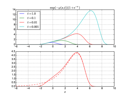
Figure 1: Top: the integrand from (10) when $\beta=1/2$ for different $t$. Bottom: comparison between the integrands from (5) and (10) when $t=0.001$; the dashed line is the former and the solid line the latter.

Section 4 introduces an alternative approach based on the substitution $p=\exp(x-e^{-x})$, which transforms (4) into the integral representation

$$\frac{1}{t^{\beta}}=\frac{1}{\Gamma(\beta)}\int_{-\infty}^{\infty}\exp\bigl{(}-\varphi(x,t)\bigr{)}(1+e^{-x})\,dx,$$ (10)

where

$$\varphi(x,t)=tp-\beta\log p=t\exp(x-e^{-x})-\beta(x-e^{-x}).$$ (11)

Applying the infinite trapezoidal rule again leads to an approximation of the form (6), this time with

$$a_{n}=\exp\bigl{(}nh-e^{-nh}\bigr{)}\quad\text{and}\quad w_{n}=h(1+e^{-nh})\exp\bigl{(}\beta(nh-e^{-nh})\bigr{)}.$$ (12)

As $x\to\infty$, the integrands in both (5) and (10) decay like $\exp(-te^{x})$. However, they exhibit different behaviours as $x\to-\infty$, with the former decaying like $e^{\beta x}=e^{-\beta|x|}$ whereas the latter decays much faster, like $\exp(-\beta e^{-x})=\exp(-\beta e^{|x|})$, as seen in Figure 1 (note the differing scales on the vertical axis).

Li Li2010 summarised several alternative approaches for fast evaluation of a fractional integral of order $\alpha$, that is, for an integral operator of the form (1) with kernel

$$k(t)=\frac{t^{\alpha-1}}{\Gamma(\alpha)}=\frac{\sin\pi\alpha}{\pi}\int_{0}^{\infty}e^{-pt}p^{-\alpha}\,dp\quad\text{for $0<\alpha<1$ and $t>0$,}$$ (13)

where the integral representation follows from (4), with $\beta=1-\alpha$, and the reflection formula for the Gamma function, $\Gamma(\alpha)\Gamma(1-\alpha)=\pi/\sin\pi\alpha$. She developed a quadrature approximation,

$$\int_{0}^{\infty}e^{-pt}p^{-\alpha}\,dp\approx\sum_{j=1}^{Q}w_{j}e^{-p_{j}t}p_{j}^{-\alpha}\quad\text{for $\delta\leq t<\infty$,}$$ (14)

which again provides an exponential sum approximation, and showed that the error can be made smaller than $\epsilon$ for all $t\in[\delta,\infty)$ with $Q$ of order $(\log\epsilon^{-1}+\log\delta^{-1})^{2}$.

More recently, Jiang et al. JiangEtAl2017 developed an exponential sum approximation for $t\in[\delta,T]$ using composite Gauss quadrature on dyadic intervals, applied to (5), with $Q$ of order

$$(\log\epsilon^{-1})\log\bigl{(}T\delta^{-1}\log\epsilon^{-1}\bigr{)}+(\log\delta^{-1})\log\bigl{(}\delta^{-1}\log\epsilon^{-1}\bigr{)}.$$

In other applications, the kernel $k(t)$ is known via its Laplace transform,

$$\hat{k}(z)=\int_{0}^{\infty}e^{-zt}k(t)\,dt,$$

so that instead of the exponential sum (2) it is natural to seek a sum-of-poles approximation,

$$\hat{k}(z)\approx\sum_{l=1}^{L}\frac{w_{l}}{z-b_{l}}$$

for $z$ in a suitable region of the complex plane; see, for instance, Alpert, Greengard and Hagstrom AlpertGreengardHagstrom2000 and Xu and Jian XuJiang2013 .

2 Approximation based on the substitution $p=e^{x}$

The nature of the approximation (6) is revealed by a remarkable formula for the relative error (BeylkinMonzon2010, , Section 2). For completeness, we outline the proof.

Theorem 2.1

If the exponents and weights are given by (7), then the relative error (8) has the representation

$$\rho(t)=-2\sum_{n=1}^{\infty}R(n/h)\cos\bigl{(}2\pi(n/h)\log t-\Phi(n/h)\bigr{)}$$ (15)

where $R(\xi)$ and $\Phi(\xi)$ are the real-valued functions defined by

$$\frac{\Gamma(\beta+i2\pi\xi)}{\Gamma(\beta)}=R(\xi)e^{i\Phi(\xi)}\quad\text{with $R(\xi)>0$ and $\Phi(0)=0$.}$$

Moreover, $R(\xi)\leq e^{-2\pi\theta|\xi|}/(\cos\theta)^{\beta}$ for $0\leq\theta<\pi/2$ and $-\infty<\xi<\infty$.

Proof

For each $t>0$, the integrand $f(x)=\exp(-te^{x}+\beta x)$ from (5) belongs to the Schwarz class of rapidly decreasing $C^{\infty}$ functions, and we may therefore apply the Poisson summation formula to conclude that

$$h\sum_{n=-\infty}^{\infty}f(nh)=\sum_{n=-\infty}^{\infty}\tilde{f}(n/h)=\int_{-\infty}^{\infty}f(x)\,dx+\sum_{n\neq 0}\tilde{f}(n/h),$$

where the Fourier transform of $f$ is

$$\tilde{f}(\xi)=\int_{-\infty}^{\infty}e^{-i2\pi\xi x}f(x)\,dx=\int_{-\infty}^{\infty}\exp\bigl{(}-te^{x}+(\beta-i2\pi\xi)x\bigr{)}\,dx.$$

The substitution $p=te^{x}$ gives

$$\tilde{f}(\xi)=\frac{1}{t^{\beta-i2\pi\xi}}\int_{0}^{\infty}e^{-p}p^{\beta-i2\pi\xi}\,\frac{dp}{p}=\frac{\Gamma(\beta-i2\pi\xi)}{t^{\beta-i2\pi\xi}},$$

so, with $a_{n}$ and $w_{n}$ defined by (7),

$$\frac{1}{\Gamma(\beta)}\sum_{n=-\infty}^{\infty}w_{n}e^{-a_{n}t}=\frac{1}{t^{\beta}}+\frac{1}{t^{\beta}}\sum_{n\neq 0}\frac{\Gamma(\beta-i2\pi n/h)}{\Gamma(\beta)}\,t^{i2\pi n/h}.$$

The formula for $\rho(t)$ follows after noting that $\overline{\Gamma(\beta+i2\pi\xi)}=\Gamma(\beta-i2\pi\xi)$ for all real $\xi$; hence, $R(-\xi)=R(\xi)$ and $\Phi(-\xi)=-\Phi(\xi)$.

To estimate $R(\xi)$, let $y>0$ and define the ray $\mathcal{C}_{\theta}=\{\,se^{i\theta}:0<s<\infty\,\}$. By Cauchy’s theorem,

$$\Gamma(\beta+iy)=\int_{\mathcal{C}_{\theta}}e^{-p}p^{\beta+iy}\,\frac{dp}{p}=\int_{0}^{\infty}e^{-se^{i\theta}}(se^{i\theta})^{\beta+iy}\,\frac{ds}{s}$$

and thus

$$|\Gamma(\beta+iy)|\leq\int_{0}^{\infty}e^{-s\cos\theta}e^{-\theta y}s^{\beta}\,\frac{ds}{s}=\frac{e^{-\theta y}}{(\cos\theta)^{\beta}}\int_{0}^{\infty}e^{-s}s^{\beta}\,\frac{ds}{s}=\frac{e^{-\theta y}}{(\cos\theta)^{\beta}}\,\Gamma(\beta),$$

implying the desired bound for $R(\xi)$.

In practice, the amplitudes $R(n/h)$ decay so rapidly with $n$ that only the first term in the expansion (15) is significant. For instance, since (AbramowitzStegun1965, , 6.1.30)

$$\bigl{|}\Gamma(\tfrac{1}{2}+iy)\bigr{|}^{2}=\frac{\pi}{\cosh(\pi y)},$$

if $\beta=1/2$ then $R(\xi)=(\cosh 2\pi^{2}\xi)^{-1/2}\leq\sqrt{2}e^{-\pi^{2}\xi}$ so, choosing $h=1/3$, we have $R(1/h)=1.95692\times 10^{-13}$ and $R(2/h)=2.70786\times 10^{-26}$. In general, the bound $R(n/h)\leq e^{-2\pi\theta n/h}/(\cos\theta)^{\beta}$ from the theorem is minimized by choosing $\tan\theta=2\pi n/(\beta h)$, implying that

$$R(n/h)\leq\bigl{(}1+(r_{n}/\beta)^{2}\bigr{)}^{\beta/2}\exp\bigl{(}-r_{n}\arctan(r_{n}/\beta)\bigr{)}\quad\text{where $r_{n}=2\pi n/h$.}$$

Since we can evaluate only a finite exponential sum, we now estimate the two tails of the infinite sum in terms of the upper incomplete Gamma function,

$$\Gamma(\beta,q)=\int_{q}^{\infty}e^{-p}p^{\beta}\,\frac{dp}{p}\quad\text{for $\beta>0$~{}and $q>0$.}$$

Theorem 2.2

If the exponents and weights are given by (7), then

$$t^{\beta}\sum_{n=N+1}^{\infty}w_{n}e^{-a_{n}t}\leq\Gamma(\beta,te^{Nh})\quad\text{provided $te^{Nh}\geq\beta$,}$$

and

$$t^{\beta}\sum_{n=-\infty}^{-M-1}w_{n}e^{-a_{n}t}\leq\Gamma(\beta)-\Gamma(\beta,te^{-Mh})\quad\text{provided $te^{-Mh}\leq\beta$.}$$

Proof

For each $t>0$, the integrand $f(x)=\exp(-te^{x}+\beta x)$ from (5) decreases for $x>\log(\beta/t)$. Therefore, if $Nh\geq\log(\beta/t)$, that is, if $te^{Nh}\geq\beta$, then

$$t^{\beta}h\sum_{n=N+1}^{\infty}f(nh)\leq t^{\beta}\int_{Nh}^{\infty}f(x)\,dx=\int_{te^{Nh}}^{\infty}e^{-p}p^{\beta}\,\frac{dp}{p}=\Gamma(\beta,te^{Nh}),$$

where, in the final step, we used the substitution $p=te^{x}$. Similarly, the function $f(-x)=\exp(-te^{-x}-\beta x)$ decreases for $x>\log(t/\beta)$ so if $Mh\geq\log(t/\beta)$, that is, if $te^{-Mh}\leq\beta$, then

$$t^{\beta}h\sum_{n=-\infty}^{-M-1}f(nh)=t^{\beta}h\sum_{n=M+1}^{\infty}f(-nh)\leq t^{\beta}\int_{Mh}^{\infty}f(-x)\,dx=\int_{0}^{te^{-Mh}}e^{-p}p^{\beta}\,\frac{dp}{p},$$

where, in the final step, we used the substitution $p=te^{-x}$.

Given $\epsilon_{\text{RD}}>0$ there exists $h>0$ such that

$$2\sum_{n=1}^{\infty}|\Gamma(\beta+i2\pi n/h)|=\epsilon_{\text{RD}}\Gamma(\beta),$$ (16)

and by Theorem 2.1,

$$|\rho(t)|\leq\epsilon_{\text{RD}}\quad\text{for $0<t<\infty$,}$$

so $\epsilon_{\text{RD}}$ is an upper bound for the relative discretization error. Similarly, given a sufficiently small $\epsilon_{\text{RT}}>0$, there exist $x_{\delta}>0$ and $X_{T}>0$ such that $\delta e^{x_{\delta}}\geq\beta$ and $Te^{-X_{T}}\leq\beta$ with

$$\Gamma(\beta,\delta e^{x_{\delta}})=\epsilon_{\text{RT}}\Gamma(\beta)\quad\text{and}\quad\Gamma(\beta)-\Gamma(\beta,Te^{-X_{T}})=\epsilon_{\text{RT}}\Gamma(\beta).$$ (17)

Thus, by Theorem 2.2,

$$\frac{t^{\beta}}{\Gamma(\beta)}\sum_{n=N+1}^{\infty}w_{n}e^{-a_{n}t}\leq\epsilon_{\text{RT}}\quad\text{for $t\geq\delta$~{}and $Nh\geq x_{\delta}$,}$$

and

$$\frac{t^{\beta}}{\Gamma(\beta)}\sum_{n=-\infty}^{-M-1}w_{n}e^{-a_{n}t}\leq\epsilon_{\text{RT}}\quad\text{for $t\leq T$ and $Mh\geq X_{T}$,}$$

showing that $2\epsilon_{\text{RT}}$ is an upper bound for the relative truncation error. Denoting the overall relative error for the finite sum (9) by

$$\rho^{N}_{M}(t)=1-\frac{t^{\beta}}{\Gamma(\beta)}\sum_{n=-M}^{N}w_{n}e^{-a_{n}t},$$ (18)

we therefore have

$$|\rho^{N}_{M}(t)|\leq\epsilon_{\text{RD}}+2\epsilon_{\text{RT}}\quad\text{for $\delta\leq t\leq T$, $Nh\geq x_{\delta}$ and $Mh\geq X_{T}$.}$$ (19)

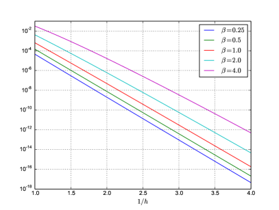
Figure 2: The bound $\epsilon_{\text{RD}}$ for the relative discretization error, defined by (16), as a function of $1/h$ for various choices of $\beta$.

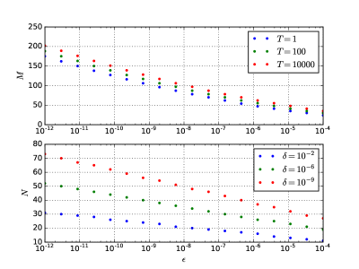
Figure 3: The growth in $M$ and $N$ as the upper bound for the overall relative error (18) decreases, for different choices of $T$ and $\delta$.

The estimate for $R(\xi)$ in Theorem 2.1, together with the asymptotic behaviours

$$\Gamma(\beta,q)\sim q^{\beta-1}e^{-q}\quad\text{as~{}$q\to\infty$},$$

and

$$\Gamma(\beta)-\Gamma(\beta,q)\sim\frac{q^{\beta}}{\beta}\quad\text{as $q\to 0$,}$$

imply that (19) can be satisfied with

$$h^{-1}\geq C\log\epsilon_{\text{RD}}^{-1},\qquad N\geq Ch^{-1}\log(\delta^{-1}\log\epsilon_{\text{RT}}^{-1}),\qquad M\geq Ch^{-1}\log(T\epsilon_{\text{RT}}^{-1}).$$

Figure 2 shows the relation between $\epsilon_{\text{RD}}$ and $1/h$ given by (16), and confirms that $1/h$ is approximately proportional to $\log\epsilon_{\text{RT}}^{-1}$. In Figure 3, for each value of $\epsilon$ we computed $h$ by solving (16) with $\epsilon_{\text{RD}}=\epsilon/3$, then computed $x_{\delta}$ and $X_{T}$ by solving (17) with $\epsilon_{\text{RT}}=\epsilon/3$, and finally put $M=\lceil X_{T}/h\rceil$ and $N=\lceil x_{\delta}/h\rceil$.

3 Prony’s method

The construction of Section 2 leads to an exponential sum approximation (9) with many small exponents $a_{n}$. We will now explain how the corresponding terms can be aggregated to yield a more efficient approximation.

Consider more generally an exponential sum

$$g(t)=\sum_{l=1}^{L}w_{l}e^{-a_{l}t},$$

in which the weights and exponents are all strictly positive. Our aim is to approximate this function by an exponential sum with fewer terms,

$$g(t)\approx\sum_{k=1}^{K}\tilde{w}_{k}e^{-\tilde{a}_{k}t},\quad 2K-1<L,$$

whose weights $\tilde{w}_{k}$ and exponents $\tilde{a}_{k}$ are again all strictly positive. To this end, let

$$g_{j}=(-1)^{j}g^{(j)}(0)=\sum_{l=1}^{L}w_{l}a_{l}^{j}.$$

We can hope to find $2K$ parameters $\tilde{w}_{k}$ and $\tilde{a}_{k}$ satisfying the $2K$ conditions

$$g_{j}=\sum_{k=1}^{K}\tilde{w}_{k}\tilde{a}_{k}^{j}\quad\text{for $0\leq j\leq 2K-1$,}$$ (20)

so that, by Taylor expansion,

$$g(t)\approx\sum_{j=0}^{2K-1}g_{j}\,\frac{(-t)^{j}}{j!}=\sum_{k=1}^{K}\tilde{w}_{k}\sum_{j=0}^{2K-1}\frac{(-\tilde{a}_{k}t)^{j}}{j!}\approx\sum_{k=1}^{K}\tilde{w}_{k}e^{-\tilde{a}_{k}t}.$$

The approximations here require that the $g_{j}$ and the $\tilde{a}_{k}t$ are nicely bounded, and preferably small.

In Prony’s method, we seek to satisfy (20) by introducing the monic polynomial

$$Q(z)=\prod_{k=1}^{K}(z-\tilde{a}_{k})=\sum_{k=0}^{K}q_{k}z^{k},$$

and observing that the unknown coefficients $q_{k}$ must satisfy

$$\sum_{m=0}^{K}g_{j+m}q_{m}=\sum_{m=0}^{K}\sum_{k=1}^{K}\tilde{w}_{k}\tilde{a}_{k}^{j+m}q_{m}=\sum_{k=1}^{K}\tilde{w}_{k}\tilde{a}_{k}^{j}\sum_{m=0}^{K}q_{m}\tilde{a}_{k}^{m}=\sum_{k=1}^{K}\tilde{w}_{k}\tilde{a}_{k}^{j}Q(\tilde{a}_{k})=0,$$

for $0\leq j\leq K-1$ (so that $j+m\leq 2K-1$ for $1\leq m\leq K$), with $q_{K}=1$. Thus,

$$\sum_{m=0}^{K-1}g_{j+m}q_{m}=b_{j},\quad\text{where $b_{j}=-g_{j+K}$,}\quad\text{for $0\leq j\leq K-1$,}$$

which suggests the procedure Prony defined in Algorithm 1. We must, however, beware of several potential pitfalls:

1. the best choice for $K$ is not clear;

2. the $K\times K$ matrix $[g_{j+k}]$ might be badly conditioned;

3. the roots of the polynomial $Q(z)$ might not all be real and positive;

4. the linear system for the $\tilde{w}_{k}$ is overdetermined, and the least-squares solution might have large residuals;

5. the $\tilde{w}_{k}$ might not all be positive.

We will see that nevertheless the algorithm can be quite effective, even when $K=1$, in which case we simply compute

$$g_{0}=\sum_{l=1}^{L}w_{l},\quad g_{1}=\sum_{l=1}^{L}w_{l}a_{l},\quad\tilde{a}_{1}=g_{1}/g_{0},\quad\tilde{w}_{1}=g_{0}.$$

Algorithm 1 $\textit{Prony}(a_{1},\dots,a_{L},w_{1},\dots w_{L},K)$

0:  $2K-1\leq L$

  Compute $g_{j}=\sum_{l=1}^{L}w_{l}a_{l}^{j}$ for $0\leq j\leq 2K-1$

  Find $q_{0}$, …, $q_{K-1}$ satisfying $\sum_{m=0}^{K-1}g_{j+m}q_{m}=-g_{j+K}$ for $0\leq j\leq K-1$, and put $q_{K}=1$

  Find the roots $\tilde{a}_{1}$, …, $\tilde{a}_{K}$ of the polynomial $Q(z)=\sum_{k=0}^{K}q_{k}z^{k}$

  Find $\tilde{w}_{1}$, …, $\tilde{w}_{K}$ satisfying $\sum_{k=1}^{K}\tilde{a}_{k}^{j}\tilde{w}_{k}\approx g_{j}$ for $0\leq j\leq 2K-1$

  return  $\tilde{a}_{1}$, …, $\tilde{a}_{K}$, $\tilde{w}_{1}$, …, $\tilde{w}_{K}$

Table 1: Performance of Prony’s method for different $L$ and $K$ using the parameters of Example 1. For each $K$, we seek the largest $L$ for which the maximum relative error is less than $\epsilon=10^{-8}$.

$\quad L\quad$	$\quad K=1\quad$	$\quad K=2\quad$	$\quad K=3\quad$	$\quad K=4\quad$	$\quad K=5\quad$	$\quad K=6\quad$
66	9.64e-01	4.30e-01	6.15e-02	3.02e-03	4.77e-05	2.29e-07
65	8.11e-01	1.69e-01	9.89e-03	1.80e-04	9.98e-07	1.66e-09
64	5.35e-01	4.59e-02	1.03e-03	6.85e-06	1.35e-08	7.96e-12
63	2.72e-01	9.17e-03	7.76e-05	1.89e-07	1.36e-10	2.74e-14
62	1.12e-01	1.46e-03	4.64e-06	4.19e-09	1.11e-12	3.58e-16
61	3.99e-02	1.98e-04	2.38e-07	8.05e-11	8.28e-15	3.52e-16
60	1.28e-02	2.43e-05	1.10e-08	1.41e-12	4.63e-16	2.24e-16
59	3.82e-03	2.78e-06	4.81e-10	2.36e-14	4.63e-16	1.25e-16
58	1.10e-03	3.05e-07	2.02e-11	4.46e-16	1.23e-16	6.27e-17
57	3.07e-04	3.27e-08	8.25e-13	5.60e-17	8.40e-17
56	8.43e-05	3.44e-09	3.32e-14	8.96e-17	5.60e-17
55	2.29e-05	3.59e-10	1.32e-15	4.48e-17	4.48e-17
48	2.30e-09	3.98e-17	2.58e-18
47	6.16e-10	3.92e-18	1.54e-18

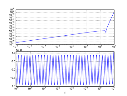
Figure 4: Top: the additional contribution $|\eta(t)|$ to the relative error from applying Prony’s method in Example 1 with $L=65$ and $K=6$. Bottom: the overall relative error for the resulting approximation (22) of $t^{-\beta}$ requiring $L-K=59$ fewer terms.

Example 1

We took $\beta=3/4$, $\delta=10^{-6}$, $T=10$, $\epsilon=10^{-8}$, $\epsilon_{\text{RD}}=0.9\times 10^{-8}$ and $\epsilon_{RT}=0.05\times 10^{-8}$. The methodology of Section 2 led to the choices $h=0.47962$, $M=65$ and $N=36$, and we confirmed via direct evaluation of the relative error that $|\rho^{N}_{M}(t)|\leq 0.92\times 10^{-8}$ for $\delta\leq t\leq T$. We applied Prony’s method to the first $L$ terms of the sum in (9), that is, those with $-M\leq n\leq L-M$, thereby reducing the total number of terms by $L-K$. Table 1 lists, for different choices of $L$ and $K$, the additional contribution to the relative error, that is, $\max_{1\leq p\leq P}|\eta(t_{p})|$ where

$$\eta(t)=\frac{t^{\beta}}{\Gamma(\beta)}\biggl{(}\sum_{k=1}^{K}\tilde{w}_{k}e^{-\tilde{a}_{k}t}-\sum_{l=1}^{L}w_{l^{\prime}}e^{-a_{l^{\prime}}t}\biggr{)},\qquad l^{\prime}=l-M+1,$$ (21)

and we use a geometric grid in $[\delta,1]$ given by $t_{p}=T^{(p-1)/(P-1)}\delta^{(P-p)/(P-1)}$ for $1\leq p\leq P$ with $P=751$. The largest reduction consistent with maintaining overall accuracy was when $L=65$ and $K=6$, and Figure 4 (Top) plots $|\eta(t)|$ in this case, as well as the overall relative error (Bottom) for the resulting approximation,

$$\frac{1}{t^{\beta}}\approx\frac{1}{\Gamma(\beta)}\biggl{(}\sum_{k=1}^{K}\tilde{w}_{k}e^{-\tilde{a}_{k}t}+\sum_{n=L-M}^{N}w_{n}e^{-a_{n}t}\biggr{)}\quad\text{for $10^{-6}\leq t\leq 10$.}$$ (22)

In this way, the number of terms in the exponential sum approximation was reduced from $M+1+N=102$ to $(M+K-L)+1+N=43$, with the maximum absolute value of the relative error growing only slightly to $1.07\times 10^{-8}$. Figure 4 (Bottom) shows that the relative error is closely approximated by the first term in (15), that is, $\rho^{M}_{N}(t)\approx-2R(h^{-1})\cos\bigl{(}2\pi h^{-1}\log t-\Phi(h^{-1})\bigr{)}$ for $\delta\leq t\leq T$.

4 Approximation based on the substitution $p=\exp(x-e^{-x})$

We now consider the alternative exponents and weights given by (12). A different approach is needed for the error analysis, and we define

$$\mathcal{I}(f)=\int_{-\infty}^{\infty}f(x)\,dx\quad\text{and}\quad\mathcal{Q}(f,h)=h\sum_{n=-\infty}^{\infty}f(nh)\quad\text{for $h>0$,}$$

so that $\mathcal{Q}(f,h)$ is an infinite trapezoidal rule approximation to $\mathcal{I}(f)$. Recall the following well-known error bound.

Theorem 4.1

Let $r>0$. Suppose that $f(z)$ is continuous on the closed strip $|\Im z|\leq r$, analytic on the open strip $|\Im z|<r$, and satisfies

$$\int_{-\infty}^{\infty}\bigl{(}|f(x+ir)|+|f(x-ir)|\bigr{)}\,dx\leq A_{r}$$

with

$$\int_{-r}^{r}|f(x\pm iy)|\,dy\to 0\quad\text{as $|x|\to\infty$.}$$

Then, for all $h>0$,

$$|\mathcal{Q}(f,h)-\mathcal{I}(f)|\leq\frac{A_{r}e^{-2\pi r/h}}{1-e^{-2\pi r/h}}.$$

Proof

See McNamee, Stenger and Whitney (McNameeEtAl1971, , Theorem 5.2).

For $t>0$, we define the entire analytic function of $z$,

$$f(z)=\exp\bigl{(}-\varphi(z,t)\bigr{)}(1+e^{-z}),$$ (23)

where $\varphi(z,t)$ is the analytic continuation of the function defined in (11). In this way, $t^{-\beta}=\mathcal{I}(f)/\Gamma(\beta)$ by (10).

Lemma 1

If $0<r<\pi/2$, then the function $f$ defined in (23) satisfies the hypotheses of Theorem 4.1 with $A_{r}\leq Ct^{-\beta}$ for $0<t\leq 1$, where the constant $C>0$ depends only on $\beta$ and $r$.

Proof

A short calculation shows that

$$\Re\varphi(x\pm iy,t)=t\exp(x-e^{-x}\cos y)\cos(y+e^{-x}\sin y)-\beta(x-e^{-x}\cos y),$$

and that if $0<\epsilon<\pi/2-r$, then

$$0\leq y+e^{-x}\sin y\leq\frac{\pi}{2}-\epsilon\quad\text{for $x\geq x^{*}=\log\frac{\sin r}{\pi/2-r-\epsilon}$ and $0\leq y\leq r$.}$$ (24)

Thus, if $x\geq x^{*}$ then $\cos(r+e^{-x}\sin r)\geq\cos(\pi/2-\epsilon)=\sin\epsilon$ so

$$\Re\varphi(x\pm ir,t)\geq t\exp(x-e^{-x^{*}}\cos r)\sin\epsilon-\beta x+\beta e^{-x}\cos r\geq cte^{x}-\beta x,$$

where $c=\exp(-e^{-x^{*}}\cos r)\sin\epsilon>0$. If necessary, we increase $x^{*}$ so that $x^{*}>0$. Since $|1+e^{-(x\pm ir)}|\leq 1+e^{-x}$,

$$\int_{x^{*}}^{\infty}|f(x\pm ir)|\,dx =\int_{x^{*}}^{\infty}\exp\bigl{(}-\Re\varphi(x\pm ir,t)\bigr{)}\bigl{|}1+e^{-(x\pm ir)}\bigr{|}\,dx$$

$$\leq\int_{x^{*}}^{\infty}\exp(-cte^{x}+\beta x)(1+e^{-x})\,dx,$$

and the substitution $p=e^{x}$ then yields, with $p^{*}=e^{x^{*}}$,

$$\int_{x^{*}}^{\infty}|f(x\pm ir)|\,dx\leq\int_{p^{*}}^{\infty}e^{-ctp}p^{\beta}(1+p^{-1})\,\frac{dp}{p}\leq\bigl{(}1+(p^{*})^{-1}\bigr{)}\int_{p^{*}}^{\infty}e^{-ctp}p^{\beta}\,\frac{dp}{p}\\ =\frac{1+(p^{*})^{-1}}{(ct)^{\beta}}\int_{ctp^{*}}^{\infty}e^{-p}p^{\beta}\,\frac{dp}{p}\leq\frac{1+(p^{*})^{-1}}{(ct)^{\beta}}\int_{0}^{\infty}e^{-p}p^{\beta}\,\frac{dp}{p}\equiv Ct^{-\beta}.$$

Also, if $x\geq 0$ then

$$\Re\varphi(x\pm ir,t)\geq-t\exp(x-e^{-x}\cos r)-\beta(x-e^{-x}\cos r)\geq-te^{x}-\beta x$$

so

$$\int_{0}^{x^{*}}|f(x\pm ir)|\,dx\leq\int_{0}^{x^{*}}\exp(te^{x}+\beta x)(1+e^{-x})\,dx\leq 2x^{*}\exp\bigl{(}te^{x^{*}}+\beta x^{*}\bigr{)},$$

which is bounded for $0<t\leq 1$. Similarly, if $x\leq 0$ then $\exp(x-e^{-x}\cos r)\leq 1$ so $\Re\varphi(x\pm ir,t)\geq-t+\beta e^{-x}\cos r$ and therefore, using again the substitution $p=e^{x}$,

$$\int_{-\infty}^{0}|f(x\pm ir)|\,dx \leq\int_{-\infty}^{0}\exp(t-\beta e^{-x}\cos r)(1+e^{-x})\,dx$$

$$=\int_{0}^{\infty}\exp(t-\beta e^{x}\cos r)(1+e^{x})\,dx=e^{t}\int_{1}^{\infty}e^{-\beta p\cos r}(1+p)\,\frac{dp}{p},$$

which is also bounded for $0<t\leq 1$. The required estimate for $A_{r}$ follows.

If $x\geq x^{*}$, then the preceding inequalities based on (24) show that

$$\int_{-r}^{r}|f(x+iy)|\,dy\leq 2r\max_{|y|\leq r}|f(x+iy)|\leq 2r\exp(-cte^{x}+\beta x)(1+e^{-x}),$$

which tends to zero as $x\to\infty$ for any $t>0$. Similarly, if $x\leq 0$, then $\Re\varphi(x\pm iy)\geq-t+\beta e^{-x}\cos r$ for $|y|\leq r$, so

$$\int_{-r}^{r}|f(x+iy)|\,dy\leq 2r\exp(t-\beta e^{-x}\cos r)(1+e^{-x}),$$

which again tends to zero as $x\to-\infty$.

Together, Theorem 4.1 and Lemma 1 imply the following bound for the relative error (8) in the infinite exponential sum approximation (6).

Theorem 4.2

Let $h>0$ and define $a_{n}$ and $w_{n}$ by (12). If $0<r<\pi/2$, then there exists a constant $C_{1}$ (depending on $\beta$ and $r$) such that

$$|\rho(t)|\leq C_{1}e^{-2\pi r/h}\quad\text{for $0<t\leq 1$.}$$

Proof

The definitions above mean that $hf(nh)=w_{n}e^{-a_{n}t}$.

Thus, a relative accuracy $\epsilon$ is achieved by choosing $h$ of order $1/\log\epsilon^{-1}$. Of course, in practice we must compute a finite sum, and the next lemma estimates the two parts of the associated truncation error.

Lemma 2

Let $h>0$, $0<\theta<1$ and $0<t\leq 1$. Then the function $f$ defined in (23) satisfies

$$\frac{h}{\Gamma(\beta)}\sum_{M=-\infty}^{-M-1}f(nh)\leq C_{2}\exp(-\beta e^{Mh})\quad\text{for}\quad Mh\geq\begin{cases}\log(\beta^{-1}-1),&0<\beta<1/2,\\ 0,&\beta\geq 1/2,\end{cases}$$ (25)

and

$$\frac{h}{\Gamma(\beta)}\sum_{n=N+1}^{\infty}f(nh)\leq\frac{C_{3}}{t^{\beta}}\,\exp\bigl{(}-\theta te^{Nh-1}\bigr{)}\quad\text{for}\quad Nh\geq 1+\log(\beta t^{-1}).$$ (26)

When $0<\beta\leq 1$, the second estimate holds also with $\theta=1$.

Proof

If $n\leq 0$, then $\varphi(nh,t)\geq-t+\beta e^{-nh}$ so

$$f(nh)\leq g_{1}(-nh)\quad\text{where}\quad g_{1}(x)=\exp(t-\beta e^{x})(1+e^{x}).$$

The function $g_{1}(x)$ decreases for $x>\log(\beta^{-1}-1)$ if $0<\beta<1/2$, and for all $x\geq 0$ if $\beta\geq 1/2$, so

$$h\sum_{n=-\infty}^{-M-1}f(nh)\leq h\sum_{n=M+1}^{\infty}g_{1}(nh)\leq\int_{Mh}^{\infty}g_{1}(x)\,dx\quad\text{for $M$ as in~{}\eqref{eq: Mh},}$$

and the substitution $p=e^{x}$ gives

$$\int_{Mh}^{\infty}g_{1}(x)\,dx=\int_{e^{Mh}}^{\infty}e^{t-\beta p}(1+p)\,\frac{dp}{p}\leq 2e^{t}\int_{e^{Mh}}^{\infty}e^{-\beta p}\,dp=\frac{2e^{t}}{\beta}\exp(-\beta e^{Mh}),$$

so the first estimate holds with $C_{2}=2e/\Gamma(\beta+1)$.

If $n\geq 0$ we have $\varphi(nh,t)\geq t\exp(nh-1)-\beta nh$ and $1+e^{-nh}\leq 2$, so

$$f(nh)\leq g_{2}(nh)\quad\text{where}\quad g_{2}(x)=2\exp(-te^{x-1}+\beta x).$$

The function $g_{2}(x)$ decreases for $x>1+\log(\beta t^{-1})$, so

$$h\sum_{n=N+1}^{\infty}f(nh)\leq\int_{Nh}^{\infty}g_{2}(x)\,dx\quad\text{for $N$ as in \eqref{eq: Nh},}$$

and the substitution $p=e^{x}$ gives

$$\int_{Nh}^{\infty}g_{2}(x)\,dx\leq 2\int_{e^{Nh}}^{\infty}e^{-te^{-1}p}p^{\beta}\,\frac{dp}{p}\\ =2\biggl{(}\frac{e}{t}\biggr{)}^{\beta}\int_{te^{Nh-1}}^{\infty}e^{-p}p^{\beta-1}\,dp.$$

Since $te^{Nh-1}\geq\beta$, if $0<\beta\leq 1$ then the integral on the right is bounded above by $\beta^{\beta-1}\exp(-te^{Nh-1})$. If $\beta>1$, then $p^{\beta-1}e^{-(1-\theta)p}$ is bounded for $p>0$ so

$$\int_{te^{Nh-1}}^{\infty}e^{-p}p^{\beta-1}\,dp=\int_{te^{Nh-1}}^{\infty}e^{-\theta p}(p^{\beta-1}e^{-(1-\theta)p})\,dp\leq C\exp(-\theta te^{Nh-1}),$$

completing the proof.

It is now a simple matter to see that the number of terms $L=M+1+N$ needed to ensure a relative accuracy $\epsilon$ for $\delta\leq t\leq 1$ is of order $(\log\epsilon^{-1})\log(\delta^{-1}\log\epsilon^{-1})$.

Theorem 4.3

Let $a_{n}$ and $w_{n}$ be defined by (12). For $0<\delta\leq 1$ and for a sufficiently small $\epsilon>0$, if

$$\frac{1}{h}\geq\frac{1}{2\pi r}\,\log\frac{3C_{1}}{\epsilon},\quad M\geq\frac{1}{h}\,\log\biggl{(}\frac{1}{\beta}\,\log\frac{3C_{2}}{\epsilon}\biggr{)},\quad N\geq 1+\frac{1}{h}\,\log\biggl{(}\frac{1}{\theta\delta}\,\log\frac{3C_{3}}{\epsilon}\biggr{)},$$

then

$$|\rho^{N}_{M}(t)|\leq\epsilon\quad\text{for $\delta\leq t\leq 1$.}$$

Proof

The inequalities for $h$, $M$ and $N$ imply that each of $C_{1}e^{-2\pi r/h}$, $C_{2}\exp(-\beta e^{Mh})$ and $C_{3}\exp(-\theta te^{Nh-1})$ is bounded above by $\epsilon t^{-\beta}/3$, so the error estimate is a consequence of Theorem 4.2, Lemma 2 and the triangle inequality. Note that the restrictions on $M$ and $N$ in (25) and (26) will be satisfied for $\epsilon$ sufficiently small.

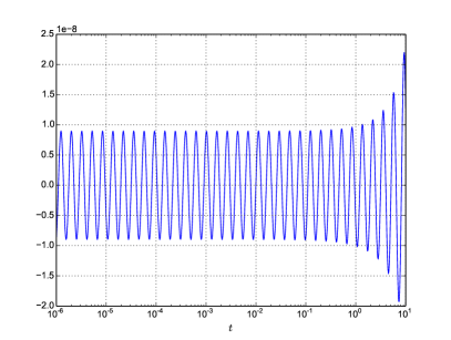
Figure 5: The relative error for the initial approximation from Example 2.

Although the error bounds above require $t\in[\delta,1]$, a simple rescaling allows us to treat a general compact subinterval $[\delta,T]$. If $\check{a}_{n}=a_{n}/T$ and $\check{w}_{n}=w_{n}/T^{\beta}$, then

$$\frac{1}{t^{\beta}}=\frac{1}{T^{\beta}}\,\frac{1}{(t/T)^{\beta}}\approx\frac{1}{\Gamma(\beta)}\sum_{n=-M}^{N}\check{w}_{n}e^{-\check{a}_{n}t}$$

for $\delta\leq t/T\leq 1$, or in other words for $\delta\cdot T\leq t\leq T$. Moreover, the relative error $\check{\rho}^{N}_{M}(t)=\rho^{N}_{M}(t/T)$ is unchanged by the rescaling.

Example 2

We took the same values for $\beta$, $\delta$, $T$, $\epsilon$, $\epsilon_{\text{RD}}$ and $\epsilon_{\text{RT}}$ as in Example 1. Since the constant $C_{1}$ of Theorem 4.2 is difficult to estimate, we again used (16) to choose $h=0.47962$. Likewise, the constant $C_{3}$ in Lemma 2 is difficult to estimate, so we chose $N=\lceil h^{-1}x_{\delta/T}\rceil=40$. However, knowing $C_{2}=2e/\Gamma(\beta+1)$ we easily determined that $C_{2}\exp(-\beta e^{Mh})\leq\epsilon_{\text{RT}}$ for $M=8$. The exponents and weights (12) were computed for the interval $[\delta/T,1]$, and then rescaled as above to create an approximation for the interval $[\delta,T]$ with $M+1+N=49$ terms and a relative error whose magnitude is at worst $2.2\times 10^{-8}$.

The behaviour of the relative error $\rho^{N}_{M}(t)$, shown in Figure 5, suggests a modified strategy: construct the approximation for $[\delta,10T]$ but use it only on $[\delta,T]$. We found that doing so required $N=45$, that is, 5 additional terms, but resulted in a nearly uniform amplitude for the relative error of about $0.97\times 10^{-8}$. Finally, after applying Prony’s method with $L=17$ and $K=6$ we were able to reduce the number of terms from $M+1+N=54$ to $43$ without increasing the relative error.

To compare these results with those of Li Li2010 , let $0<\alpha<1$ and let $k(t)=t^{\alpha-1}/\Gamma(\alpha)$ denote the kernel for the fractional integral of order $\alpha$. Taking $\beta=1-\alpha$ we compute the weights $w_{l}$ and exponents $a_{l}$ as above and define

$$k_{M}^{N}(t)=\frac{1}{\Gamma(\alpha)\Gamma(1-\alpha)}\sum_{n=-M}^{N}w_{n}e^{-a_{n}t}\quad\text{for $\delta\leq t\leq T$.}$$

The fast algorithm evaluates

$$(\mathcal{K}_{M}^{N}U)^{n}=\int_{0}^{t_{n-1}}k^{N}_{M}(t-s)\tilde{U}(s)\,ds+\int_{t_{n-1}}^{t_{n}}k(t_{n}-s)\tilde{U}(s)\,ds$$

and our bound $|\rho^{N}_{M}(t)|\leq\epsilon$ implies that $|k_{M}^{N}(t)-k(t)|\leq\epsilon t^{\alpha-1}/\Gamma(\alpha)$ for $\delta\leq t\leq T$, so

$$\bigl{|}(\mathcal{K}_{M}^{N}U)^{n}-(\mathcal{K}\tilde{U})(t_{n})\bigr{|}\leq\epsilon\int_{0}^{t_{n-1}}\frac{(t_{n}-s)^{\alpha-1}}{\Gamma(\alpha)}\,|\tilde{U}(s)|\,ds\leq\frac{\epsilon t_{n}^{\alpha}}{\Gamma(\alpha+1)}\,\max_{1\leq j\leq n}|U^{j}|,$$

provided $\Delta t_{n}\geq\delta$ and $t_{n}\leq T$. Similarly, the method of Li yields $(\mathcal{K}_{Q}U)^{n}$ but with a bound for the absolute error in (14), so that $|k_{Q}(t)-k(t)|\leq\epsilon^{\prime}$ for $\delta^{\prime}\leq t<\infty$. Thus,

$$\bigl{|}(\mathcal{K}_{Q}U)^{n}-(\mathcal{K}\tilde{U})(t_{n})\bigr{|}\leq\epsilon^{\prime}\,\frac{\sin\pi\alpha}{\pi}\int_{0}^{t_{n-1}}\,|\tilde{U}(s)|\,ds\leq\epsilon^{\prime}t_{n}\,\frac{\sin\pi\alpha}{\pi}\,\max_{1\leq j\leq n}|U^{j}|,$$

provided $\Delta t_{n}\geq\delta$. Li (Li2010, , Fig. 3 (d)) required about $Q=250$ points to achieve an (absolute) error $\epsilon^{\prime}\leq 10^{-6}$ for $t\geq\delta^{\prime}=10^{-4}$ when $\alpha=1/4$ (corresponding to $\beta=1-\alpha=3/4$). In Examples 1 and 2, our methods give a smaller error $\epsilon\leq 10^{-8}$ using only $M+1+N=43$ terms with a less restrictive lower bound for the time step, $\delta=10^{-6}$. Against these advantages, the method of Li permits arbitrarily large $t_{n}$.

5 Conclusion

Comparing Examples 1 and 2, we see that, for comparable accuracy, the approximation based on the second substitution results in far fewer terms because we are able to use a much smaller choice of $M$. However, after applying Prony’s method both approximations are about equally efficient. If Prony’s method is not used, then the second approximation is clearly superior. Another consideration is that the first approximation has more explicit error bounds so we can more easily determine suitable choices of $h$, $M$ and $N$ to achieve a desired accuracy.

References

(1)
Abramowitz, M., Stegun, I.A.: Handbook of Mathematical Functions.
Dover (1965)
(2)
Alpert, B., Greengard, L., Hagstrom, T.: Rapid evaluation of nonreflecting
boundary kernels for time-domain wave propogation.
SIAM J. Numer. Anal. 37, 1138–1164 (2000).
DOI 10.1137/S0036142998336916
(3)
Beylkin, G., Monzón, L.: Approximation by exponential sums revisited.
Appl. Comput. Harmon. Anal. 28, 131–149 (2010).
DOI 10.1016/j.acha.2009.08.011
(4)
Jiang, S., Zhang, J., Zhang, Q., Zhang, Z.: Fast evaluation of the Caputo
fractional derivative and its applications to fractional diffusion equations.
Communications in Computational Physics 21(3), 650–678
(2017).
DOI 10.4208/cicp.OA-2016-0136
(5)
Li, J.R.: A fast time stepping method for evaluating fractional integrals.
SIAM J. Sci. Comput. 31, 4696–4714 (2010).
DOI 10.1137/080736533
(6)
McNamee, J., Stenger, F., Whitney, E.L.: Whittaker’s cardinal function in
retrospect.
Math. Comp. 25, 141–154 (1971).
DOI 10.2307/2005140
(7)
Xu, K., Jiang, S.: A bootstrap method for sum-of-poles approximations.
J. Sci. Comput. 55, 16–39 (2013).
DOI 10.1007/s10915-012-9620-9