$n=200$		$n=400$		$n=800$
		PseudoNet	CONCORD	PseudoNet	CONCORD	PseudoNet	CONCORD
AUC	Median	0.68	0.65	0.81	0.73	0.91	0.86
	IQR	0.02	0.01	0.01	0.01	0.01	0.01
Squared Frobenius norm	Median	6391.48	20150.68	5722.84	18805.59	4205.49	14990.35
	IQR	84.70	513.99	26.18	245.65	18.22	192.78
$\ell_{2}$ operator norm	Median	2.51	5.17	2.41	5.07	2.56	5.84
	IQR	0.01	0.06	0.01	0.03	0.01	0.03
Elementwise $\ell_{1}$ norm	Median	17480.45	35959.79	21640.10	46951.74	21749.16	51526.46
	IQR	65.71	323.46	35.01	240.09	26.38	276.32
Elementwise $\ell_{\infty}$ norm	Median	1.34	2.93	1.06	2.32	0.67	1.38
	IQR	0.01	0.04	0.01	0.02	0.01	0.03
Wallclock time (secs.)	Median	73.72	103.23	40.76	71.02	14.60	20.46
	IQR	3.23	41.53	1.76	29.54	0.70

Table 1: Median and interquartile range for PseudoNet and CONCORD’s areas under the curves (AUCs), estimation errors in several matrix norms, and wallclock times ($p=1000$). Higher median AUC is better, lower median estimation error and wallclock time is better; best in bold. PseudoNet outperforms CONCORD across all sample sizes and metrics.

We also investigate the efficacy of PseudoNet’s screening rules; using the same synthetic data, we measure the (median across 50 trials) percentages of variables that the rules suggest dropping (excluding diagonal entries), as well as the percentages of violations (for $\lambda_{2}=1$). Figure 3.2 presents the results: the rules drop more variables as $\lambda_{1}$ increases (as expected), but never commit any violations.

Figure 1: Percentages of dropped variables excluding diagonal entries (dashed line, right vertical axes) and violations (solid line, left vertical axes) for PseudoNet’s screening rules ($\lambda_{2}=1$). First row is $p=1000$, second row is $p=3000$; first column is $n=0.2p$, second is $n=0.4p$, third is $n=0.8p$. The rules never commit a violation.

3.2 Minimum variance portfolio optimization

Next, we evaluate PseudoNet, as well as several other methods, in the context of a finance application. We consider the problem of minimum variance portfolio optimization, i.e., we must allocate our wealth across $p$ assets so that our overall risk is minimized; we model risk here as $x^{T}\hat{\Sigma}x$, where $x\in{\mbox{\bf R}}^{p}$ is an allocation vector ($x_{i}>0$ corresponds to a long position, while $x_{i}<0$ corresponds to a short position), and $\hat{\Sigma}$ is an estimate of the underlying covariance matrix. This leads to the following (convex) optimization problem:

$$\begin{array}[]{ll}\underset{x\in{\bf R}^{p}}{\mathop{\mbox{minimize}}}&x^{T}\hat{\Sigma}x\\ \mbox{subject to}&\mathbf{1}^{T}x=1,\end{array}$$

which admits the analytical solution $x=(\mathbf{1}^{T}\hat{\Sigma}^{-1}\mathbf{1})^{-1}\hat{\Sigma}^{-1}\mathbf{1}$. We choose to solve a minimum variance portfolio optimization problem (instead of, say, a mean/variance problem (Markowitz, 1952)) in order to isolate the impact of the estimate $\hat{\Omega}=\hat{\Sigma}^{-1}$.

We obtained the closing prices of the 30 constituent stocks of the Dow Jones Industrial Average (DJIA) from February 18, 1995 through October 26, 2012 (roughly 17 years) from http://finance.yahoo.com. We divided the data into $T=261$ consecutive time periods (of roughly 20 days each). The $H$ days preceding each trading period, commonly referred to as the estimation horizon, were used to compute the estimate $\hat{\Omega}$; 10-fold cross-validation using the criterion (LABEL:eq:bic) was used to choose $\lambda_{1}$ and $\lambda_{2}$. The trading period was then used to evaluate the methods. We investigated $H\in\{35,40,45,50,75,150,225,300\}$.

We primarily evaluated each method using realized risk, i.e.,

$$r=\left((1/T)\sum_{t=1}^{T}\left(x_{t}^{T}p_{t}-\bar{p}\right)^{2}\right)^{1/2},$$

where $x_{t},p_{t}\in{\mbox{\bf R}}^{p}$ are the portfolio allocation and price change vectors for period $t$, respectively, and $\bar{p}$ is the realized return, i.e.,

$$\bar{p}=(1/T)\sum_{t=1}^{T}x_{t}^{T}p_{t},$$

as well as the (commonly used) Sharpe ratio, i.e.,

$$\left(\bar{p}-p_{\textrm{free}}\right)/r,$$

where $p_{\textrm{free}}$ is the risk-free rate (we set $p_{\textrm{free}}=5\%$); intuitively, realized risk measures the instability (i.e., riskiness) of a trading strategy, and the Sharpe ratio trades off the (risk-free rate adjusted) returns and risk.

We compared PseudoNet with CONCORD, the sample covariance matrix (denoted Sample), the GLasso, the condition number-regularized inverse covariance matrix estimator of Won et al. (2013) (CondReg), the Ledoit-Wolf estimator (Ledoit and Wolf, 2003) (Ledoit), as well as the DJIA itself (i.e., an index fund). Tables 3.2 and 3.2 present the results. When the estimation horizon is small, i.e., when $H\in\{35,40,45,50,75\}$, PseudoNet achieves the lowest risk, which is a useful feature when markets fluctuate; PseudoNet is always within 4% of the lowest risk when the estimation horizon is larger. Additionally, PseudoNet achieves significantly lower risk than CONCORD across all estimation horizons. These reductions in risk also translate into better Sharpe ratios for PseudoNet: PseudoNet achieves the highest Sharpe ratio four (out of eight) times, which is more than any other method. When PseudoNet does not achieve the highest Sharpe ratio, it is usually within 5% of the best Sharpe ratio. We also plot the cumulative wealth (in $) achieved by an estimator (for $H=300$) in Figure 2. PseudoNet achieves the highest cumulative wealth despite not (directly) optimizing for returns ($8.75 for PseudoNet versus $8.72 for CONCORD) while incurring less risk: PseudoNet also preserves the most wealth during the 2008–2009 financial crisis ($4.64 for PseudoNet versus $4.43 for CONCORD and $4.23 for CondReg). Further details are provided in the supplement.

Table 3: Realized risk for various estimators and estimation horizons $H$ in the portfolio optimization example. Lower is better; best in bold. PseudoNet is best 5/8 times.

Table 4: Sharpe ratios for various estimators and estimation horizons $H$ in the portfolio optimization example. Higher is better; best in bold. PseudoNet is best 4/8 times.

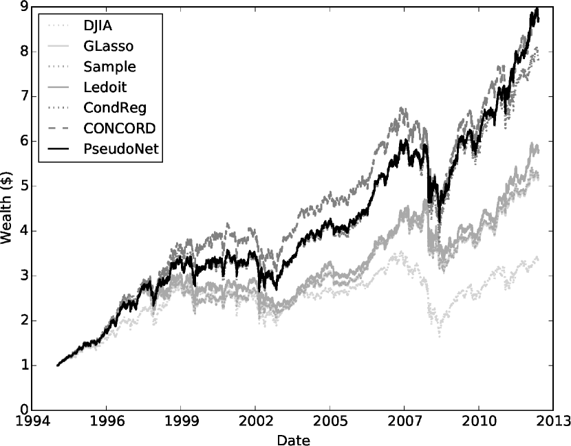
Figure 2: Cumulative wealth for various estimators in the portfolio optimization example ($H=300$); higher is better. PseudoNet achieves the highest cumulative wealth.

3.3 Sustainable energy application

Finally, we evaluate PseudoNet on the task of recovering the conditional independencies between several wind farms on the basis of historical wind power measurements at these farms; wind power is naturally intermittent (as are many renewable resources), and thus understanding the relationships between wind farms can help operators forecast, plan, and dispatch. We obtained hourly wind power measurements from July 1, 2009 through September 14, 2010 (440 days) at seven wind farms from http://www.kaggle.com/c/GEF2012-wind-forecasting; see Hong et al. (2014) for further details, as well as a summary of a recent Kaggle competition based on this data. Each group of 48 columns in the data set corresponds to two days (i.e., 48 hours) of hourly wind power measurements at a particular farm; to model the nonlinear relationship between wind power at different locations, we consider five radial basis function kernels spread evenly and evaluated at each hourly measurement (see, for example, Wytock and Kolter (2013); Ali et al. (2016) for a similar approach). Thus, $p=7\times 48\times 5=1680$. Each row in the data set considers wind power measurements starting 12 hours after the (start of the) previous row; for example, the first row considers wind power measurements from 1:00 pm on July 1, 2009 through 12:00 pm on July 3, 2009, the second row from 1:00 am on July 2, 2009 through 12:00 am on July 4, 2009, and the last row from 1:00 am on September 12, 2010 through 12:00 am on September 14, 2010. Thus, $n=877$. Computing the PseudoNet estimate here therefore corresponds to learning the structure of a spatiotemporal graphical model.

The left panel of Figure 3 presents the PseudoNet estimate’s sparsity pattern. The nonzero super- and sub-diagonal entries suggest that at any wind farm the previous hour’s wind power (naturally) influences the next hour’s, while the nonzero off-diagonal entries, for example, in the (4,6) block, uncover farms that may influence one another: for example, farms 4 and 6 may be nearby, or (perhaps more interestingly) they may not be nearby. Wytock and Kolter (2013), whose method placed fifth in the Kaggle competition, as well as Ali et al. (2016) report similar findings (see the left panel of Figure 7 as well as Figure S.3, respectively, in these papers). The right panel of Figure 3 evaluates PseudoNet’s screening rules on this data set: the rules never commit a violation.

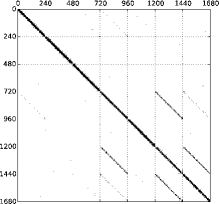
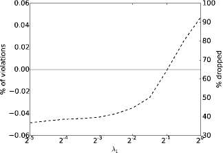
Figure 3: Left: sparsity pattern for the PseudoNet estimate (black means nonzero, and each block corresponds to a wind farm). Right: percentages of dropped variables excluding diagonal entries (dashed line, right vertical axes) and violations (solid line, left vertical axes) for PseudoNet’s screening rules ($\lambda_{2}=1$); the rules never commit a violation.

4 Theory

Finally, we collect here all our theoretical results on PseudoNet’s statistical and computational properties. We state these results, essentially, in the order in which they are referenced in the text above. Accordingly, we first show that the PseudoNet estimator converges to the unique, global solution of its defining optimization problem at a geometric (“linear”) rate. Following this, we show, under suitable regularity conditions, that PseudoNet is consistent at a rate of $\sqrt{(\log p)/n}$; additionally, we provide a two-step method that obtains accurate estimates of the diagonal entries of the underlying inverse covariance matrix, even when $p>n$, as required by our consistency proof, which goes beyond the consistency proofs for the related pseudolikelihood-based estimators SPACE (Peng et al., 2009, Theorem 3) and CONCORD (Khare et al., 2015, Theorem 2). Finally, we show that the PseudoNet estimate does not saturate, while the SPLICE, SPACE, and CONCORD estimates can saturate. As a reminder, all proofs can be found in the supplement.

4.1 Linear convergence

We begin by showing that Algorithm LABEL:alg:ours, used to compute the PseudoNet estimate, converges to the unique, global solution of the PseudoNet optimization problem (LABEL:eq:ours) at a geometric (“linear”) rate; this constrasts with a number of other pseudolikelihood-based methods, which do not provide unique estimates (Rocha et al., 2008; Peng et al., 2009; Friedman et al., 2010; Khare et al., 2015; Oh et al., 2014), making interpretation difficult, are not guaranteed to converge (Rocha et al., 2008; Peng et al., 2009; Friedman et al., 2010), or converge at a slower rate (Khare et al., 2015; Oh et al., 2014).

The result is given in Lemma 4.1 below.

Lemma 4.1 (Linear convergence).

Suppose $\Omega^{(0)},\ldots,\Omega^{(k)}$ is a sequence of PseudoNet iterates with nonincreasing objective value. Let $\hat{\Omega}^{\textrm{net}}$ be the solution of the PseudoNet optimization problem (LABEL:eq:ours). Then we get that

$$\|\Omega^{(i)}-\hat{\Omega}^{\textrm{net}}\|_{F}\leq(1-c)^{i}\|\Omega^{(0)}-\hat{\Omega}^{\textrm{net}}\|_{F},\quad i=1,\ldots,k,$$

where $c=\lambda_{2}/L$ and $L$ is the Lipschitz constant for the gradient of the smooth term $\nabla g$ in (LABEL:eq:prox2).

4.2 Consistency

Next, we show, under suitable regularity conditions, that PseudoNet is consistent at a rate of $\sqrt{(\log p)/n}$. Previous consistency results on pseudolikelihood-based estimators assume the existence of accurate estimates of the diagonal entries of the underlying inverse covariance matrix $\Omega^{0}$; however, no method for obtaining such estimates is provided in these papers when $p>n$ (Khare et al., 2015; Peng et al., 2009). Below, we provide a two-step method that obtains accurate diagonal estimates, which are required for the PseudoNet consistency proof (as well as for the consistency proofs for CONCORD and SPACE); this is done in Theorem 4.3.

We now provide the regularity conditions required to establish the consistency of PseudoNet; the assumptions are essentially the same as those required in Khare et al. (2015), which are in turn similar to those in Peng et al. (2009).

1. Sub-Gaussian rows. We require that the rows of the data matrix $X$ are i.i.d. sub-Gaussian random vectors, i.e., there exists a constant $c\geq 0$ such that, for all $t\in{\mbox{\bf R}}^{p}$, we have that $\mathop{\bf E{}}\exp(t^{T}X_{i\cdot})\leq\exp((c^{2}/2)t^{T}t),\;i=1,\ldots,n$, where, as a reminder, $X_{i\cdot}$ is the $i$th row of $X$.

2. Correlation restrictions. For all $n$, we require that the minimum and maximum eigenvalues of the underlying covariance matrix $\Sigma^{0}$, i.e., $\lambda_{\min}(\Sigma^{0})$ and $\lambda_{\max}(\Sigma^{0})$, are uniformly bounded away from zero and infinity (note that we omit the notational dependence of $\Sigma^{0}$, as well as some related quantities, on $n$, for simplicity).

3. Incoherence. We require that there exists a constant $\alpha<1$ such that, for all $(i,j)\in\mathcal{A}_{n}^{c}$, where $\mathcal{A}_{n}$ here is the support of the off-diagonal entries of the underlying inverse covariance matrix $\Omega^{0}_{\textrm{off}}$, i.e.,

   $$\mathcal{A}_{n}=\left\{(i,j):1\leq i<j\leq p,\;\Omega^{0}_{ij}\neq 0\right\},$$

   we have that

   $$\left|\bar{L}_{ij,\mathcal{A}_{n}}^{{}^{\prime\prime}}(\omega^{0}_{\textrm{off}},\omega^{0}_{\textrm{diag}})(\bar{L}_{\mathcal{A}_{n}\mathcal{A}_{n}}^{{}^{\prime\prime}}(\omega^{0}_{\textrm{off}},\omega^{0}_{\textrm{diag}}))^{-1}\mathop{\bf sign}\omega^{0}_{\mathcal{A}_{n}}\right|\leq\alpha.$$ (8)

   Here, the $\mathop{\bf sign}$ here is interpreted elementwise; $\omega^{0}_{\textrm{off}}$ and $\omega^{0}_{\textrm{diag}}$ are the vectorizations of the off-diagonal and diagonal entries, respectively, of the underlying inverse covariance matrix $\Omega^{0}$, i.e.,

   $$\omega^{0}_{\textrm{off}}=\mathop{\bf vec}\Omega^{0}_{\textrm{off}},\quad\omega^{0}_{\textrm{diag}}=\mathop{\bf vec}\Omega^{0}_{\textrm{diag}};$$

   $L(\omega_{\textrm{off}}^{0},\omega_{\textrm{diag}}^{0})$ equals the $\log\det$ plus trace terms in (LABEL:eq:ours) evaluated at $(\omega_{\textrm{off}}^{0},\omega_{\textrm{diag}}^{0})$, i.e.,

   $$L(\omega_{\textrm{off}}^{0},\omega_{\textrm{diag}}^{0})=-(1/2)\log\det((\Omega^{0}_{\textrm{diag}})^{2})+(n/2)\mathop{\bf Tr}(S(\Omega^{0})^{2});$$

   and $\bar{L}^{{}^{\prime\prime}}_{ij,k\ell}(\omega_{\textrm{off}}^{0},\omega_{\textrm{diag}}^{0})$ is an element of the negative $(p^{2}\times p^{2})$-dimensional Fisher information matrix at $(\omega_{\textrm{off}}^{0},\omega_{\textrm{diag}}^{0})$, i.e.,

   $$\bar{L}^{{}^{\prime\prime}}_{ij,k\ell}(\omega_{\textrm{off}}^{0},\omega_{\textrm{diag}}^{0})=\mathop{\bf E{}}\frac{\partial^{2}L(\omega_{\textrm{off}}^{0},\omega_{\textrm{diag}}^{0})}{\partial\omega_{\textrm{off},ij}^{0}\omega_{\textrm{off},k\ell}^{0}},\quad i,j,k,\ell=1,\ldots,p$$

   (we abuse notation somewhat and write $\omega_{ij}=\Omega_{ij}$).

4. Accurate diagonal estimates. We require the existence of accurate diagonal estimates $\hat{\omega}_{\textrm{diag}}$ such that

   $$\|\hat{\omega}_{\textrm{diag}}-\omega^{0}_{\textrm{diag}}\|_{\infty}=O_{P}(\sqrt{(\log n)/n}).$$

   As stated in the beginning of this subsection, a method to obtain such estimates is provided in Theorem 4.3; our two-step method firstly performs a lasso regression (with tuning parameter $\lambda_{1,n}$) of each diagonal element on the remaining variables to identify subsets of relevant variables, and secondly estimates each diagonal element with the variance of the residuals given by the linear regression of each diagonal element on its subset of relevant variables.

5. Support size and tuning parameter restrictions. As $n\to\infty$, we let $q_{n}=o(\sqrt{n/\log n})$, $\lambda_{1,n}\sqrt{q_{n}}\to 0$, $\lambda_{1,n}\sqrt{n/\log n}\to\infty$, and $\lambda_{2,n}=o(\lambda_{1,n})$, where $q_{n}=|\mathcal{A}_{n}|$ (note that we make explicit here the notational dependence of the tuning parameters on $n$).

6. Signal restrictions. As $n\to\infty$, we require that $s_{n}/(\lambda_{1,n}\sqrt{q_{n}})\to\infty$, where $s_{n}=\max_{(i,j)\in\mathcal{A}_{n}}|\omega^{0}_{\textrm{off},ij}|$.

Condition (iii) can be interpreted as requiring bounded correlation between the rows of $\bar{L}_{\mathcal{A}_{n}^{c}\mathcal{A}_{n}}^{{}^{\prime\prime}}(\omega^{0}_{\textrm{off}},\omega^{0}_{\textrm{diag}})$ and the columns of $(\bar{L}_{\mathcal{A}_{n}\mathcal{A}_{n}}^{{}^{\prime\prime}}(\omega^{0}_{\textrm{off}},\omega^{0}_{\textrm{diag}}))^{-1}$. Khare et al. (2015) as well as Peng et al. (2009) also use this condition; see Khare et al. (2015) for examples that satisfy this condition.

The following theorem presents our consistency result for PseudoNet.

Theorem 4.2 (Consistency).

Assume the conditions stated above. Let $p=O(n^{\kappa})$ for a constant $\kappa>0$, and let $\hat{\Omega}^{\textrm{net}}$ be the PseudoNet estimate given by the solution of the PseudoNet optimization problem (LABEL:eq:ours). Then, we have, with probability at least $1-O(n^{-\beta})$ for a constant $\beta>0$,

1. signed support recovery: $\mathop{\bf sign}\hat{\omega}^{\textrm{net}}_{ij}=\mathop{\bf sign}\omega^{0}_{ij},\;i,j=1,\ldots,p$, where $\hat{\omega}^{\textrm{net}}=\mathop{\bf vec}\hat{\Omega}^{\textrm{net}}$ (we take $\mathop{\bf sign}0=0$)

2. estimation error: $\|\hat{\omega}^{\textrm{net}}-\omega^{0}\|_{2}\leq c_{1}\lambda_{1,n}\sqrt{q_{n}}$, for a constant $c_{1}>0$.

4.2.1 Accurate diagonal estimates

The following theorem provides consistent estimates of the diagonal entries of the underlying inverse covariance matrix $\Omega^{0}$. In the case when $d_{n}$, which denotes the maximum number of nonzero entries in any row of $\Omega^{0}$, is bounded in $n$, this theorem yields estimates satisfying condition (iv) above, even when $p>n$; this result is also useful in the context of consistency for CONCORD (Khare et al., 2015, Theorem 2) and SPACE (Peng et al., 2009, Theorem 3), where such diagonal estimates are assumed, but a method to obtain them is not provided.

Theorem 4.3 (Accurate diagonal estimates via two-step method).

Assume conditions (i), (ii), (v), and (vi) above. Assume further that there exists a constant $\delta<1$ such that

$$\left|\Sigma^{0}_{i,\mathcal{A}_{n}^{j}}\left(\Sigma^{0}_{\mathcal{A}_{n}^{j},\mathcal{A}_{n}^{j}}\right)^{-1}\mathop{\bf sign}\Omega^{0}_{\mathcal{A}_{n}^{j},j}\right|\leq\delta,\quad i\notin\mathcal{A}_{n}^{j},\;j=1,\ldots,p,$$ (9)

where

$$d_{n} =\max_{k=1,\ldots,p}\left|\left\{\ell:\ell\in\{1,\ldots,p\},\;\ell\neq k,\;\Omega^{0}_{k\ell}\neq 0\right\}\right|,$$

$$\mathcal{A}_{n}^{j} =\left\{k:k\in\{1,\ldots,p\},\;k\neq j,\;\Omega^{0}_{jk}\neq 0\right\},$$

and the $\mathop{\bf sign}$ in (9) is interpreted elementwise. Now, for $j=1,\ldots,p$, let $\hat{\mathcal{A}}^{j}_{n}$ be the set of indices corresponding to the nonzero coefficients obtained by fitting a lasso regression of the $j$th diagonal element on the remaining variables (with tuning parameter $\lambda_{1,n}$). Also, let $\hat{\omega}_{\textrm{diag},j}$ be the sample variance of the $j$th diagonal element conditioned on the variables in $\hat{\mathcal{A}}^{j}_{n}$. Then, for every $\beta>0$, there exists a constant $c_{2}>0$ such that

$$\|\hat{\omega}_{\textrm{diag}}-\omega^{0}_{\textrm{diag}}\|_{\infty}\leq c_{2}d_{n}\sqrt{(\log n)/n},$$

with probability at least $1-O(n^{-\beta})$.

We note that (9) is similar but not equivalent to condition (iii) above.

4.3 Saturation

Lastly, we show that the PseudoNet estimate does not saturate (i.e., when $p\gg n$, the number of variables selected by PseudoNet can be greater than $np$ out of $p(p-1)/2$ total variables), while the SPLICE, SPACE, and CONCORD estimates can saturate; this is rather limiting for these latter estimators from the points of view of both estimation error as well as interpretability.

To do this, we first introduce some notation that makes the statements of these results, as well as their proofs, more concise. We use $\mathop{\bf vech}$ to mean the half-vectorization operator, i.e., the concatenation of the lower triangle of its (matrix) argument, excluding diagonal entries. We use $\mathop{\bf card}$ to count the number of nonzero entries in its argument. Also, we say that the columns of a wide matrix $A\in{\mbox{\bf R}}^{k\times\ell}$ (i.e., $\ell>k$) are in general position if the affine span of any $m\leq k$ signed columns of $A$, i.e., $s_{i_{1}}A_{i_{1}},\ldots,s_{i_{m}}A_{i_{m}}$, where each $s_{j},\;j=i_{1},\ldots,i_{m}$ is fixed to either $+1$ or $-1$, does not contain any of the points $\pm A_{j},\;j\neq i_{1},\ldots i_{m}$.

Below, Theorem 4.4 states our saturation results for PseudoNet and CONCORD; Corollary 4.5 then gives the analogous results for SPLICE and SPACE.

Theorem 4.4 (Saturation results for PseudoNet and CONCORD).

Let

$$A=-\left[\begin{array}[]{cccccccccccccccccccccccc}X_{2}&X_{3}&X_{4}&\cdots&X_{p-1}&X_{p}&0&\lx@intercol\hfil\cdots\hfil\lx@intercol&0\\ X_{1}&0&\lx@intercol\hfil\cdots\hfil\lx@intercol&0&X_{3}&X_{4}&X_{5}&\cdots&X_{p-1}&X_{p}&0&\lx@intercol\hfil\cdots\hfil\lx@intercol&0\\ 0&X_{1}&0&\lx@intercol\hfil\cdots\hfil\lx@intercol&0&X_{2}&0&\lx@intercol\hfil\cdots\hfil\lx@intercol&0&X_{4}&X_{5}&X_{6}&\cdots&X_{p-1}&X_{p}&0&\lx@intercol\hfil\cdots\hfil\lx@intercol&0\\ \lx@intercol\hfil\vdots\hfil\lx@intercol\\ 0&\lx@intercol\hfil\cdots\hfil\lx@intercol&0&X_{1}&0&\lx@intercol\hfil\cdots\hfil\lx@intercol&0&X_{2}&0&\lx@intercol\hfil\cdots\hfil\lx@intercol&0&X_{3}&0&\lx@intercol\hfil\cdots\hfil\lx@intercol&0&X_{p-1}\end{array}\right],$$

i.e., $A\in{\mbox{\bf R}}^{np\times p(p-1)/2}$ is a matrix containing the columns of the data matrix $X$ arranged in a particular fashion. Also, let $\hat{\Omega}^{\textrm{net}}$ be the PseudoNet estimate, i.e., the solution of the PseudoNet optimization problem (LABEL:eq:ours), and let $\hat{\Omega}^{\textrm{con}}$ be a CONCORD estimate; so, we have $\mathop{\bf vech}\hat{\Omega}^{\textrm{net}},\mathop{\bf vech}\hat{\Omega}^{\textrm{con}}\in{\mbox{\bf R}}^{p(p-1)/2}$. Assume that $p\gg n$. Then, the PseudoNet estimate does not saturate, i.e., $\mathop{\bf card}\mathop{\bf vech}\hat{\Omega}^{\textrm{net}}\leq p(p-1)/2$, and there exists a CONCORD estimate that saturates, i.e., $\mathop{\bf card}\mathop{\bf vech}\hat{\Omega}^{\textrm{con}}\leq np$. Furthermore, if the columns of the matrix $A$ are in general position, then all CONCORD estimates saturate.

The analogous results for SPLICE and SPACE follow by using arguments similar to those given in the proof of Theorem 4.4; to make the statement of these results clearer, we first describe the SPLICE and SPACE estimators in more detail.

We can obtain a SPLICE estimate by first minimizing the following objective, alternately over the variables $D\in{\mbox{\bf R}}^{p\times p}$ and $B\in{\mbox{\bf R}}^{p\times p}$, where $D$ is a diagonal matrix and the diagonal entries of the matrix $B$ are set to zero,

$$-(1/2)\log\det D+(1/2)\sum_{i=1}^{p}\frac{1}{D_{ii}^{2}}\|X_{i}-X_{-i}(B_{i\cdot})^{T}\|_{2}^{2}+\lambda_{1}\|B\|_{1},$$ (10)

where $X_{-i}$ denotes the data matrix $X$ after removing the $i$th column, and $B_{i\cdot}$ here means the $i$th row of $B$ after removing the entry $B_{ii}$; then, for any iteration $i$, we compute the estimate

$$\hat{\Omega}^{\textrm{spl},(i)}=(\hat{D}^{(i-1)})^{-2}(I-\hat{B}^{(i)}),$$ (11)

with $\hat{\Omega}^{\textrm{spl},(i)}$ referring to the estimate at the end of the $i$th iteration ($\hat{D}^{(i-1)}$ and $\hat{B}^{(i)}$ are interpreted similarly).

Turning to SPACE, we can compute a SPACE estimate by minimizing the following objective, alternately over the variables $\Omega_{\textrm{diag}}$ and $\Omega_{\textrm{off}}$,

$$-(1/2)\log\det\Omega_{\textrm{diag}}+(1/2)\sum_{i=1}^{p}\Omega_{\textrm{diag},ii}\left\|X_{i}-\sum_{j\neq i}^{p}\Omega_{\textrm{off},ij}\sqrt{\Omega_{\textrm{diag},jj}/\Omega_{\textrm{diag},\;ii}}X_{j}\right\|_{2}^{2}+\lambda_{1}\|\Omega_{\textrm{off}}\|_{1},$$ (12)

where $\Omega_{\textrm{diag},ii}$ refers to the $(i,i)$th entry of $\Omega_{\textrm{diag}}$ ($\Omega_{\textrm{off},ij}$ is interpreted similarly). As a reminder, $\Omega_{\textrm{diag}}\in{\mbox{\bf R}}^{p\times p}$ is a matrix of the diagonal entries of $\Omega$, with its off-diagonal entries set to zero; $\Omega_{\textrm{off}}\in{\mbox{\bf R}}^{p\times p}$ is a matrix of the off-diagonal entries of $\Omega$, with its diagonal entries set to zero; and we form the SPACE estimate, for any iteration $i$, as $\hat{\Omega}^{\textrm{spc},(i)}=\hat{\Omega}_{\textrm{diag}}^{(i)}+\hat{\Omega}_{\textrm{off}}^{(i)}$. To be clear, the superscripts involving $i$ here are interpreted just as with SPLICE above (also, we note that in the optimization problem (12), we have set the “weights” for each regression subproblem $i$ to $\Omega_{\textrm{diag},ii}$, as recommended by Peng et al. (2009)).

Corollary 4.5 below gives the corresponding results for SPLICE and SPACE.

Corollary 4.5 (Saturation results for SPLICE and SPACE).

Let $\hat{\Omega}^{\textrm{spl},(i)}$ be a SPLICE estimate at the end of iteration $i$, i.e., a solution of the optimization problem (10) and Equation 11, and let $\hat{\Omega}^{\textrm{spc},(i)}$ be a SPACE estimate at the end of iteration $i$, i.e., a solution of the optimization problem (12); so, we have $\mathop{\bf vech}\hat{\Omega}^{\textrm{spl},(i)},\mathop{\bf vech}\hat{\Omega}^{\textrm{spc},(i)}\in{\mbox{\bf R}}^{p(p-1)/2}$. Assume that $p\gg n$. Then, there exist SPLICE and SPACE estimates at the end of iteration $i$ that saturate, i.e., $\mathop{\bf card}\mathop{\bf vech}\hat{\Omega}^{\textrm{spl},(i)}\leq np$ and $\mathop{\bf card}\mathop{\bf vech}\hat{\Omega}^{\textrm{spc},(i)}\leq np$.

5 Discussion

We introduced PseudoNet, a new, more flexible pseudolikelihood-based estimator of the inverse covariance matrix; PseudoNet can be viewed as generalizing several Gaussian likelihood-based, as well as pseudolikelihood-based, estimators in ways that give PseudoNet a number of statistical and computational advantages. We showed, through a number of experiments, that PseudoNet significantly outperforms the closely related CONCORD estimator, in terms of both estimation error and variable selection accuracy, and that PseudoNet deals effectively with non-Gaussian data, making it well-suited for use in downstream applications. We also showed, under regularity conditions, that PseudoNet is consistent at a rate of $\sqrt{(\log p)/n}$; our proof assumes the existence of accurate estimates of the diagonal entries of the underlying inverse covariance matrix (like SPACE and CONCORD), and also provides a two-step method to obtain these estimates, even when $p>n$ (going beyond SPACE and CONCORD). Unlike several other pseudolikelihood-based methods, we also showed that the PseudoNet estimate does not saturate (i.e., when $p\gg n$, the number of variables selected by PseudoNet can be greater than $np$ out of $p(p-1)/2$ total variables), which is useful from both the perspectives of estimation error and interpretability. We presented a fast algorithm for computing the PseudoNet estimate; we showed that this algorithm converges at a geometric (“linear”) rate to the unique, global solution of the PseudoNet optimization problem, and that it is faster than CONCORD. Finally, we presented sequential strong screening rules that make computing the PseudoNet estimate over a range of tuning parameters much more tractable. As a whole, we believe these statistical and computational properties represent a useful step forward in the design of pseudolikelihood-based estimators of the inverse covariance matrix.

Supplement to “Generalized Pseudolikelihood Methods for Inverse Covariance Estimation”

S.6 Proof of Lemma LABEL:thm:screen

Proof.

By considering the gradient of the smooth term in the objective of the PseudoNet optimization problem (LABEL:eq:ours), given by (LABEL:eq:grad), in a componentwise fashion, we can express the optimality conditions for (LABEL:eq:ours), evaluated at the off-diagonal entries of $\hat{\Omega}_{ij}^{\textrm{net}}(\lambda_{1}^{(k)},\lambda_{2}^{(\ell)})$, as

$$\begin{array}[]{llll}\left|c_{ij}(\lambda_{1}^{(k)},\lambda_{2}^{(\ell)})\right|&\leq\lambda_{1}^{(k)}&\quad\textrm{if}\quad\hat{\Omega}_{ij}^{\textrm{net}}(\lambda_{1}^{(k)},\lambda_{2}^{(\ell)})&=0\\ c_{ij}(\lambda_{1}^{(k)},\lambda_{2}^{(\ell)})&=\lambda_{1}^{(k)}&\quad\textrm{if}\quad\hat{\Omega}_{ij}^{\textrm{net}}(\lambda_{1}^{(k)},\lambda_{2}^{(\ell)})&>0\\ c_{ij}(\lambda_{1}^{(k)},\lambda_{2}^{(\ell)})&=-\lambda_{1}^{(k)}&\quad\textrm{if}\quad\hat{\Omega}_{ij}^{\textrm{net}}(\lambda_{1}^{(k)},\lambda_{2}^{(\ell)})&<0.\end{array}$$ (S.13)

But, we have that

$$\left|c_{ij}(\lambda_{1}^{(k)},\lambda_{2}^{(\ell)})\right| \leq\left|c_{ij}(\lambda_{1}^{(k)},\lambda_{2}^{(\ell)})-c_{ij}(\lambda_{1}^{(k-1)},\lambda_{2}^{(\ell)})\right|+\left|c_{ij}(\lambda_{1}^{(k-1)},\lambda_{2}^{(\ell)})\right|$$

$$<|\lambda_{1}^{(k)}-\lambda_{1}^{(k-1)}|+2\lambda_{1}^{(k)}-\lambda_{1}^{(k-1)}$$

$$=\lambda_{1}^{(k)},$$

with the first inequality following by the triangle inequality, and the second by the assumptions that the $c_{ij}$ are nonexpansive and nonincreasing, as well as the further assumption that $\left|c_{ij}(\lambda_{1}^{(k-1)},\lambda_{2}^{(\ell)})\right|<2\lambda_{1}^{(k)}-\lambda_{1}^{(k-1)}$; by checking (S.13), this implies that $\hat{\Omega}_{ij}^{\textrm{net}}(\lambda_{1}^{(k)},\lambda_{2}^{(\ell)})=0$ is a solution. ∎

S.7 Additional numerical results for the minimum variance portfolio optimization example

In addition to the numerical results given in the main paper, we consider here the realized risk and Sharpe ratios for various estimators and estimation horizons, after accounting for borrowing costs (at an 8% annual percentage rate) and transaction costs (at 0.5% of the principal); Tables S.7 and S.7 present the results, and we generally see the same trends as in the main paper. PseudoNet achieves the lowest risk when the estimation horizon is small, and otherwise is within 5% of the lowest risk. PseudoNet also achieves the highest Sharpe ratio four (out of eight) times, and is otherwise within 5% of the highest Sharpe ratio.

Table S.5: Realized risk for various estimators and estimation horizons $H$, after accounting for borrowing and transaction costs, in the portfolio optimization example. Lower is better; best in bold. PseudoNet is best 5/8 times.

Table S.6: Sharpe ratios for various estimators and estimation horizons $H$, after accounting for borrowing and transaction costs, in the portfolio optimization example. Higher is better; best in bold. PseudoNet is best 4/8 times.

Qualitatively, we find that, although PseudoNet does provide sparse estimates, these estimates are usually somewhat denser than those provided by CONCORD (as expected); Figure S.4 plots these estimates (from a randomly chosen investment horizon and trading period). Thus, owing to its (comparatively) denser and better estimates, PseudoNet can reduce risk by hedging, for example, by taking a short position in a stock whose returns are negatively correlated with another stock that it also takes a long position in. To this end, we consider the size of the short side of a portfolio $x\in{\mbox{\bf R}}^{p}$, which is defined as the ratio of the magnitude of all the short positions in the portfolio to the magnitude of the portfolio, expressed as a percentage, i.e.,

$$100\times\left(\sum_{i=1}^{p}\min\{x_{i},0\}\right)/\left(\sum_{i=1}^{p}|x_{i}|\right).$$

Table S.7 presents the size of the short side, averaged over all trading periods, for various estimators and estimation horizons, and we indeed see that the size of PseudoNet’s short side is larger than CONCORD’s, GLasso’s, and CondReg’s.

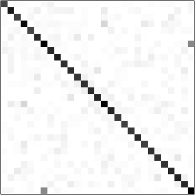
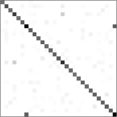
Figure S.4: Estimates provided by PseudoNet (left) and CONCORD (right); darker means larger in magnitude.

Table S.7: Average size of the short side for various estimators and estimation horizons $H$ in the portfolio optimization example.

S.8 Proof of Lemma 4.1

We prove this result by first establishing, in the following lemma, that the gradient of the smooth term in the objective in the PseudoNet optimization problem (LABEL:eq:ours), $\nabla g$, is Lipschitz continuous.

Lemma S.8.1.

Suppose $\Omega^{(0)},\ldots,\Omega^{(k)}$ is a sequence of PseudoNet iterates with nonincreasing objective value. Let $\Omega$ be any of the iterates here. Also, let $L=1/\ell^{2}+\|S\|_{2}+\lambda_{2}$, with $\|\cdot\|_{2}$ denoting the $\ell_{2}$ operator norm (maximum singular value), and $\ell$ being a constant that uniformly lower bounds $\Omega_{ii}$, $i=1,\ldots,p$. Then we get that $\nabla^{2}g(\Omega)\preceq LI_{p^{2}\times p^{2}}$.

Proof.

Let $J_{\textrm{net}}$ be the objective in the PseudoNet optimization problem (LABEL:eq:ours). Then we have that

$$-\sum_{i=1}^{p}\log\Omega_{ii}+(\lambda_{2}/2)\sum_{i=1}^{p}\Omega^{2}_{ii}\leq J_{\textrm{net}}(\Omega^{(0)}),$$

since the $\ell_{1}$ term in the objective in (LABEL:eq:ours) is nonnegative, and the trace term can be expressed as a nonnegative quadratic form. The lefthand side here approaches $\infty$ as either $\Omega_{ii}\rightarrow\infty$ or $\Omega_{ii}\rightarrow 0$, i.e., $\Omega_{ii}$ must be uniformly bounded away from $\infty$ and 0 by some $u$ and $\ell$, respectively, for $i=1,\ldots,p$, owing to the righthand side of the expression. Thus, we can upper bound the eigenvalues of (LABEL:eq:hess) with

$$1/\ell^{2}+\|S\|_{2}^{2}+\lambda_{2},$$

as claimed. ∎

Obtaining linear convergence is now immediate. As $g$ is smooth, the conclusion in Lemma S.8.1 is equivalent to $\nabla^{2}g(\Omega)\preceq LI_{p^{2}\times p^{2}}\iff\|\nabla g(\Omega)-\nabla g(\tilde{\Omega})\|_{F}\leq L\|\Omega-\tilde{\Omega}\|_{F}$, where $\tilde{\Omega}\in{\mbox{\bf S}}_{++}^{p}$, and $L=1/\ell^{2}+\|S\|_{2}+\lambda_{2}$. Now, since $g$ is also $\lambda_{2}$-strongly convex, the claim follows by Schmidt et al. (2011, Proposition 3). $\;\square$

S.9 Proof of Theorem 4.4

Proof.

We proceed by first showing that there exists a CONCORD estimate that saturates; then we show that the PseudoNet estimate does not saturate.

A CONCORD estimate is defined as a solution to the following (convex) optimization problem:

$$\begin{array}[]{ll}\underset{\Omega\in{\bf R}^{p\times p}}{\mathop{\mbox{minimize}}}&-(1/2)\log\det(\Omega_{\textrm{diag}}^{2})+(n/2)\mathop{\bf Tr}S\Omega^{2}+\lambda_{1}\|\Omega_{\textrm{off}}\|_{1},\end{array}$$ (S.14)

where, as a reminder, $\Omega_{\textrm{diag}}\in{\mbox{\bf R}}^{p\times p}$ is a matrix of the diagonal entries of $\Omega$, with its off-diagonal entries set to zero; $S\in{\mbox{\bf R}}^{p\times p}$ is the sample covariance matrix, i.e., $S=(1/n)X^{T}X$, and $X\in{\mbox{\bf R}}^{n\times p}$ is a data matrix; $\Omega_{\textrm{off}}\in{\mbox{\bf R}}^{p\times p}$ is a matrix of the off-diagonal entries of $\Omega$, with its diagonal entries set to zero; $\lambda_{1}$ is a tuning parameter; and $\|\cdot\|_{1}$ is the elementwise $\ell_{1}$ norm.

Letting

$$\tilde{J}_{\textrm{con}}(\Omega_{\textrm{diag}})=\inf_{\Omega_{\textrm{off}}}\;(1/2)\sum_{i=1}^{p}\left\|\sum_{j=1}^{p}\Omega_{ij}X_{j}\right\|_{2}^{2}+\lambda_{1}\|\Omega_{\textrm{off}}\|_{1},$$ (S.15)

we see that the optimization problem (S.14) above is equivalent to

$$\begin{array}[]{ll}\underset{\Omega_{\textrm{diag}}}{\mathop{\mbox{minimize}}}&-(1/2)\log\det(\Omega_{\textrm{diag}}^{2})+\tilde{J}_{\textrm{con}}(\Omega_{\textrm{diag}}).\end{array}$$

Next, define

$$b=\left[\begin{array}[]{c}\Omega_{11}X_{1}\\ \Omega_{22}X_{2}\\ \Omega_{33}X_{3}\\ \vdots\\ \Omega_{pp}X_{p}\end{array}\right],\quad\omega=\left[\begin{array}[]{c}\Omega_{12}\\ \Omega_{13}\\ \vdots\\ \Omega_{1p}\\ \Omega_{23}\\ \Omega_{24}\\ \vdots\\ \Omega_{2p}\\ \Omega_{34}\\ \Omega_{35}\\ \vdots\\ \Omega_{3p}\\ \vdots\\ \Omega_{p-1,p}\end{array}\right],$$

i.e., $b\in{\mbox{\bf R}}^{np}$ and $\omega=\mathop{\bf vech}\Omega\in{\mbox{\bf R}}^{p(p-1)/2}$.

Then we can express (S.15) as

$$\inf_{\omega}\;(1/2)\|b-A\omega\|_{2}^{2}+\lambda_{1}\|\omega\|_{1},$$ (S.16)

which is evidently a lasso problem with variable $\omega$.

Then, by Tibshirani (2013, Lemma 14), for any $b$, $A$, and $\lambda_{1}>0$, there exists a solution $\hat{\omega}(\Omega_{\textrm{diag}})$ of (S.16) (note that we have written here the solution $\hat{\omega}$ as a function of $\Omega_{\textrm{diag}}$ to emphasize the dependence on $\Omega_{\textrm{diag}}$) that will have at most $\min\{np,p(p-1)/2\}$ nonzero entries for any value of $\Omega_{\textrm{diag}}$; thus, when $p\gg n$, $\mathop{\bf card}\hat{\omega}(\Omega_{\textrm{diag}})\leq np$, as claimed. The final claim in the statement of the result follows by invoking Tibshirani (2013, Lemma 3).

Now, turning to the PseudoNet optimization problem (LABEL:eq:ours), we have that the trace plus the squared Frobenius norm penalty in the objective in (LABEL:eq:ours) can be expressed as

$$(n/2)\mathop{\bf Tr}S\Omega^{2}+(\lambda_{2}/2)\sum_{i,j=1}^{p}\Omega_{ij}^{2} =(1/2)\sum_{i=1}^{p}\Omega_{i}^{T}X^{T}X\Omega_{i}+(\lambda_{2}/2)\sum_{i=1}^{p}\Omega_{i}^{T}\Omega_{i}$$

$$=(1/2)\sum_{i=1}^{p}\Omega_{i}^{T}\left(X^{T}X+\lambda_{2}I\right)\Omega_{i}$$

$$=(1/2)\sum_{i=1}^{p}\left\|\sum_{j=1}^{p}\Omega_{ij}\left[\begin{array}[]{c}X_{j}\\ \sqrt{\lambda_{2}}e_{j}\end{array}\right]\right\|_{2}^{2},$$ (S.19)

where, as a reminder, $e_{i}$ is the $i$th standard basis vector in ${\mbox{\bf R}}^{p}$.

Thus, following a similar argument as above, we can express (LABEL:eq:ours) as a lasso problem with variable $\omega\in{\mbox{\bf R}}^{p(p-1)/2}$, $A\in{\mbox{\bf R}}^{p(n+p)\times p(p-1)/2}$, and $b\in{\mbox{\bf R}}^{p(n+p)}$; however, in this case, the solution $\hat{\omega}(\Omega_{\textrm{diag}})$ can have $p(p-1)/2$ nonzeros, as claimed. ∎

S.10 Proof of Corollary 4.5

We prove these results by following a strategy similar to the one we used in the proof of Theorem 4.4. Note that, at the end of some iteration $i-1$, we can consider the variables $D$ (for SPLICE) and $\Omega_{\textrm{diag}}$ (for SPACE) fixed, and then optimize over $B$ (for SPLICE) and $\Omega_{\textrm{off}}$ (for SPACE). Accordingly, we let (for SPLICE)

$$b_{\textrm{spl}}^{(i-1)}=\left[\begin{array}[]{c}(1/\hat{D}_{11}^{(i-1)})X_{1}\\ (1/\hat{D}_{22}^{(i-1)})X_{2}\\ (1/\hat{D}_{33}^{(i-1)})X_{3}\\ \vdots\\ (1/\hat{D}_{pp}^{(i-1)})X_{p}\end{array}\right],\quad\omega_{\textrm{spl}}=\left[\begin{array}[]{c}(B_{1\cdot})^{T}\\ (B_{2\cdot})^{T}\\ (B_{3\cdot})^{T}\\ \vdots\\ (B_{p\cdot})^{T}\end{array}\right],$$

$$A_{\textrm{spl}}^{(i-1)}=\left[\begin{array}[]{cccccc}(1/\hat{D}_{11}^{(i-1)})X_{-1}&0&0&0&\cdots&0\\ 0&(1/\hat{D}_{22}^{(i-1)})X_{-2}&0&0&\cdots&0\\ 0&0&(1/\hat{D}_{33}^{(i-1)})X_{-3}&0&\cdots&0\\ \lx@intercol\hfil\vdots\hfil\lx@intercol\\ 0&0&0&0&\cdots&(1/\hat{D}_{pp}^{(i-1)})X_{-p}\end{array}\right],$$

i.e., $b_{\textrm{spl}}^{(i-1)}\in{\mbox{\bf R}}^{np}$, $\omega_{\textrm{spl}}\in{\mbox{\bf R}}^{p(p-1)}$, and $A_{\textrm{spl}}^{(i-1)}\in{\mbox{\bf R}}^{np\times p(p-1)}$. We also let (for SPACE)

$$b_{\textrm{spc}}^{(i-1)}=\left[\begin{array}[]{c}\sqrt{\hat{\Omega}_{11}^{(i-1)}}X_{1}\\ \sqrt{\hat{\Omega}_{22}^{(i-1)}}X_{2}\\ \sqrt{\hat{\Omega}_{33}^{(i-1)}}X_{3}\\ \vdots\\ \sqrt{\hat{\Omega}_{pp}^{(i-1)}}X_{p}\end{array}\right],\quad\omega_{\textrm{spc}}=\left[\begin{array}[]{c}\Omega_{12}\\ \Omega_{13}\\ \vdots\\ \Omega_{1p}\\ \Omega_{23}\\ \Omega_{24}\\ \vdots\\ \Omega_{2p}\\ \Omega_{34}\\ \Omega_{35}\\ \vdots\\ \Omega_{3p}\\ \vdots\\ \Omega_{p-1,p}\end{array}\right],$$

$$A_{\textrm{spc}}^{(i-1)}=\left[\begin{array}[]{cccccccccccccccccccccccc}\tilde{X}{2}&\tilde{X}{3}&\tilde{X}{4}&\cdots&\tilde{X}{p-1}&\tilde{X}{p}&0&\lx@intercol\hfil\cdots\hfil\lx@intercol&0\\ \tilde{X}{1}&0&\lx@intercol\hfil\cdots\hfil\lx@intercol&0&\tilde{X}{3}&\tilde{X}{4}&\tilde{X}{5}&\cdots&\tilde{X}{p-1}&\tilde{X}{p}&0&\lx@intercol\hfil\cdots\hfil\lx@intercol&0\\ 0&\tilde{X}{1}&0&\lx@intercol\hfil\cdots\hfil\lx@intercol&0&\tilde{X}{2}&0&\lx@intercol\hfil\cdots\hfil\lx@intercol&0&\tilde{X}{4}&\tilde{X}{5}&\tilde{X}{6}&\cdots&\tilde{X}{p-1}&\tilde{X}{p}&0&\lx@intercol\hfil\cdots\hfil\lx@intercol&0\\ \lx@intercol\hfil\vdots\hfil\lx@intercol\\ 0&\lx@intercol\hfil\cdots\hfil\lx@intercol&0&\tilde{X}{1}&0&\lx@intercol\hfil\cdots\hfil\lx@intercol&0&\tilde{X}{2}&0&\lx@intercol\hfil\cdots\hfil\lx@intercol&0&\tilde{X}{3}&0&\lx@intercol\hfil\cdots\hfil\lx@intercol&0&\tilde{X}{p-1}\end{array}\right],$$

where we write $\tilde{X}_{j}=\sqrt{\hat{\Omega}_{jj}^{(i-1)}}X_{j}$; so, $b_{\textrm{spc}}^{(i-1)}\in{\mbox{\bf R}}^{np}$, $\omega_{\textrm{spc}}\in{\mbox{\bf R}}^{p(p-1)/2}$, and $A_{\textrm{spc}}^{(i-1)}\in{\mbox{\bf R}}^{np\times p(p-1)/2}$. Applying Tibshirani (2013, Lemma 14) as before, and noting that applying (11) does not affect the sparsity pattern of $\hat{B}^{(i)}$ for SPLICE, gives the required results.

S.11 Proof of Theorem 4.2

Proof.

Define $w_{i}=\hat{\Omega}_{ii}^{2},\;i=1,\ldots,p$, where, as a reminder, the $\hat{\Omega}_{ii}$ are estimates of the diagonal entries of $\Omega^{0}$ that are assumed in condition (iv) (see the statement of Theorem 4.2), and consider the change of variables for the off-diagonal entries of $\Omega$

$$\omega_{ij}=-\theta_{ij}(\hat{\Omega}_{ii}\hat{\Omega}_{jj})^{1/2},\quad i,j=1,\ldots,p,\;i\neq j,$$

where $\theta\in{\mbox{\bf R}}^{p(p-1)}$ and again $\omega=\mathop{\bf vec}\Omega$; then we can express the trace term in the objective in the PseudoNet optimization problem (LABEL:eq:ours) as

$$n\mathop{\bf Tr}S\Omega^{2} =\sum_{i=1}^{p}(w_{i}/\hat{\Omega}_{ii}^{2})\Omega_{i}^{T}X^{T}X\Omega_{i}$$

$$=\sum_{i=1}^{p}(w_{i}/\hat{\Omega}_{ii}^{2})\left\|\sum_{j=1}^{p}\omega_{ij}X_{j}\right\|_{2}^{2}$$

$$=\sum_{i=1}^{p}w_{i}\left\|(1/\hat{\Omega}_{ii})\left(\hat{\Omega}_{ii}X_{i}+\sum_{j\neq i}^{p}\omega_{ij}X_{j}\right)\right\|_{2}^{2}$$

$$=\sum_{i=1}^{p}w_{i}\left\|X_{i}+\sum_{j\neq i}^{p}(\omega_{ij}/\hat{\Omega}_{ii})X_{j}\right\|_{2}^{2}$$

$$=\sum_{i=1}^{p}w_{i}\left\|X_{i}-\sum_{j\neq i}^{p}\theta_{ij}\left(\hat{\Omega}_{jj}/\hat{\Omega}_{ii}\right)^{1/2}X_{j}\right\|_{2}^{2}.$$ (S.21)

Equation S.21 is equal to the objective of the SPACE optimization problem (cf. Peng et al. (2009, Equation 10) and/or the trace term in Khare et al. (2015, Equation 12)), up to constants and for fixed diagonal entries; thus, the $\log\det$ term (which is only a function of diagonal entries) plus the trace term in the objective in (LABEL:eq:ours) are also equivalent to the corresponding terms in the SPACE’s objective. This implies that properties A1–A4 and B0–B3 in the supplement for Peng et al. (2009) also apply to the $\log\det$ plus trace terms in the objective in (LABEL:eq:ours).

Now, let $L(\theta)$ denote the $\log\det$ plus trace terms in the objective in (LABEL:eq:ours) (with variable off-diagonal entries $\theta\in{\bf R}^{p(p-1)}$ and fixed diagonal entries $\hat{\omega}_{\textrm{diag}}$), and let $B_{c_{1}}(\theta_{\textrm{off}}^{0},c_{1}q_{n}^{1/2}\lambda_{1,n})$ be a ball of radius $c_{1}q_{n}^{1/2}\lambda_{1,n}$, for a constant $c_{1}>0$, with center $\theta_{\textrm{off}}^{0}$, i.e., $B_{c_{1}}=\{\theta:\|\theta-\theta^{0}_{\textrm{off}}\|_{2}\leq c_{1}q_{n}^{1/2}\lambda_{1,n}\}$, where $\theta_{\textrm{off}}^{0}$ is the application of the same (strictly monotone) transformation in (S.11) to the underlying off-diagonal entries $\omega_{\textrm{off}}^{0}$.

First, we show that the unique, global solution (owing to the strong convexity of (S.22)) of the following “restricted” optimization problem lies in $B_{c_{1}}$ with probability tending to one as $n\to\infty$:

$$\begin{array}[]{ll}\underset{\theta:\theta_{\mathcal{A}_{n}^{c}}=0}{\mathop{\mbox{minimize}}}&L(\theta)+\lambda_{1,n}\sum_{i\neq j}^{p}\left|(\hat{\Omega}_{ii}\hat{\Omega}_{jj})^{1/2}\theta_{ij}\right|+(\lambda_{2,n}/2)\sum_{i\neq j}^{p}\hat{\Omega}_{ii}\hat{\Omega}_{jj}\theta_{ij}^{2}.\end{array}$$ (S.22)

Let $\alpha_{n}=q_{n}^{1/2}\lambda_{1,n}$, and let $u\in{\mbox{\bf R}}^{p(p-1)}$ with $u_{\mathcal{A}_{n}^{c}}=0$ and $\|u\|_{2}=c$, for a constant $c>0$. Fix $\theta\in B_{c_{1}}$ to be equal to $\theta_{\textrm{off}}^{0}+\alpha_{n}u$. Then we have that

$$\lambda_{1,n}\left(\sum_{i\neq j}^{p}\left|(\hat{\Omega}_{ii}\hat{\Omega}_{jj})^{1/2}\theta_{\textrm{off},ij}^{0}\right|-\sum_{i\neq j}^{p}\left|(\hat{\Omega}_{ii}\hat{\Omega}_{jj})^{1/2}\theta_{ij}\right|\right)$$

$$\quad\leq\lambda_{1,n}\sum_{i\neq j}^{p}\left|(\hat{\Omega}_{ii}\hat{\Omega}_{jj})^{1/2}(\theta_{\textrm{off},ij}^{0}-\theta_{ij})\right|$$

$$\quad=\lambda_{1,n}\alpha_{n}\sum_{i\neq j}^{p}\left|(\hat{\Omega}_{ii}\hat{\Omega}_{jj})^{1/2}u_{ij}\right|$$

$$\quad=O(\lambda_{1,n}\alpha_{n}q_{n}^{1/2}\|u\|_{2})$$

$$\quad=O(\alpha_{n}^{2}),$$ (S.23)

with probability at least $1-O(n^{-\beta})$, as the diagonal estimates $\hat{\Omega}_{ii}$ are uniformly bounded with high probability; the second line here follows by the triangle inequality, the third by the choice of $\theta$, the fourth by the Cauchy-Schwarz inequality and the definition of $u$, and the fifth by the definition $\alpha_{n}=q_{n}^{1/2}\lambda_{1,n}$.

We also have that

$$(\lambda_{2,n}/2)\left(\sum_{i\neq j}^{p}\hat{\Omega}_{ii}\hat{\Omega}_{jj}(\theta_{\textrm{off},ij}^{0})^{2}-\sum_{i\neq j}^{p}\hat{\Omega}_{ii}\hat{\Omega}_{jj}\theta_{ij}^{2}\right)$$ (S.24)

$$\quad=(\lambda_{2,n}/2)\left(\sum_{i\neq j}^{p}\hat{\Omega}_{ii}\hat{\Omega}_{jj}(\theta_{\textrm{off},ij}^{0})^{2}-\sum_{i\neq j}^{p}\hat{\Omega}_{ii}\hat{\Omega}_{jj}(\theta_{\textrm{off},ij}^{0}+\alpha_{n}u_{ij})^{2}\right)$$

$$\quad=-\lambda_{2,n}\alpha_{n}\sum_{i\neq j}^{p}\hat{\Omega}_{ii}\hat{\Omega}_{jj}\theta_{\textrm{off},ij}^{0}u_{ij}-(\lambda_{2,n}/2)\alpha_{n}^{2}\sum_{i\neq j}^{p}\hat{\Omega}_{ii}\hat{\Omega}_{jj}u_{ij}^{2}.$$ (S.25)

We get for the first term in (S.25) that

$$-\lambda_{2,n}\alpha_{n}\sum_{i\neq j}^{p}\hat{\Omega}_{ii}\hat{\Omega}_{jj}\theta_{\textrm{off},ij}^{0}u_{ij} \leq O(\lambda_{2,n}\alpha_{n}q_{n}^{1/2})\|u\|_{2}$$

$$=o(\alpha_{n}^{2})\|u\|_{2},$$ (S.26)

with probability at least $1-O(n^{-\beta})$; the first line here follows by the Cauchy-Schwarz inequality, and the second by the assumption that $\lambda_{2,n}=o(\lambda_{1,n})$.

Similarly, we get for the second term in (S.25)

$$-(\lambda_{2,n}/2)\alpha_{n}^{2}\sum_{i\neq j}^{p}\hat{\Omega}_{ii}\hat{\Omega}_{jj}u_{ij}^{2} \leq o(\alpha_{n}^{2})\|u\|_{2}^{2},$$ (S.27)

with probability at least $1-O(n^{-\beta})$.

Putting (S.26) and (S.27) together, we get for (S.24) that

$$(\lambda_{2,n}/2)\left(\sum_{i\neq j}^{p}\hat{\Omega}_{ii}\hat{\Omega}_{jj}(\theta_{\textrm{off},ij}^{0})^{2}-\sum_{i\neq j}^{p}\hat{\Omega}_{ii}\hat{\Omega}_{jj}\theta_{ij}^{2}\right)\leq o(\alpha_{n}^{2})\left(\|u\|_{2}+\|u\|_{2}^{2}\right)$$ (S.28)

with probability at least $1-O(n^{-\beta})$.

Next, let $J_{\textrm{net}}(\theta)$ equal the objective in (LABEL:eq:ours) (with fixed diagonal entries $\hat{\omega}_{\textrm{diag}}$); combining (S.23) and (S.28), we get

$$J_{\textrm{net}}(\theta)-J_{\textrm{net}}(\theta^{0}_{\textrm{off}}) \geq L(\theta)-L(\theta_{\textrm{off}}^{0})$$

$$\quad-\lambda_{1,n}\left(\sum_{i\neq j}^{p}\left|(\hat{\Omega}_{ii}\hat{\Omega}_{jj})^{1/2}\theta_{\textrm{off},ij}^{0}\right|-\sum_{i\neq j}^{p}\left|(\hat{\Omega}_{ii}\hat{\Omega}_{jj})^{1/2}\theta_{ij}\right|\right)$$

$$\quad-(\lambda_{2,n}/2)\left(\sum_{i\neq j}^{p}\hat{\Omega}_{ii}\hat{\Omega}_{jj}(\theta_{\textrm{off},ij}^{0})^{2}-\sum_{i\neq j}^{p}\hat{\Omega}_{ii}\hat{\Omega}_{jj}\theta_{ij}^{2}\right)$$

$$\geq L(\theta)-L(\theta_{\textrm{off}}^{0})-O(\alpha_{n}^{2})-o(\alpha_{n}^{2})$$

$$=L(\theta)-L(\theta_{\textrm{off}}^{0})-O(\alpha_{n}^{2}).$$

By the same arguments in the proof of Lemma S-3 in the supplement for Peng et al. (2009), it follows that the (unique, global) solution to the restricted problem (S.22) lies in $B_{c_{1}}$, with probability at least $1-O(n^{-\beta})$; this also implies (by a simple contradiction argument) that the event $\mathop{\bf sign}\hat{\theta}_{\mathcal{A}_{n}}=\mathop{\bf sign}\theta^{0}_{\mathcal{A}_{n}}$ occurs with high probability.

By construction, the solution $\hat{\theta}$ to the restricted optimization problem (S.22) satisfies the support “block” of the optimality conditions for the unrestricted optimization problem (LABEL:eq:ours). Next, we show that $\hat{\theta}$ satisfies the non-support (the complement of the support) block of the optimality conditions for the unrestricted optimization problem (LABEL:eq:ours).

The optimality conditions for the unrestricted optimization problem (LABEL:eq:ours) are

$$\begin{array}[]{lll}L_{ij}^{{}^{\prime}}(\theta)+\lambda_{2,n}\hat{\Omega}_{ii}\hat{\Omega}_{jj}\theta_{ij}&=-\lambda_{1,n}(\hat{\Omega}_{ii}\hat{\Omega}_{jj})^{1/2}\mathop{\bf sign}\theta_{ij}&\quad\textrm{if }\theta_{ij}\neq 0\\ |L_{ij}^{{}^{\prime}}(\theta)+\lambda_{2,n}\hat{\Omega}_{ii}\hat{\Omega}_{jj}\theta_{ij}|&\leq\lambda_{1,n}(\hat{\Omega}_{ii}\hat{\Omega}_{jj})^{1/2}&\quad\textrm{if }\theta_{ij}=0,\end{array}$$ (S.29)

where $L^{{}^{\prime}}_{ij}(\theta)=\partial L(\theta)/\partial\theta_{ij}$; this establishes the analog of Lemma S-1 in the supplement for Peng et al. (2009), and also implies that Lemma S-2 there applies to the unrestricted optimization problem (LABEL:eq:ours) here. We wish to show that (with high probability)

$$\max_{(i,j)\in\mathcal{A}_{n}^{c}}|L_{ij}^{{}^{\prime}}(\hat{\theta})+\lambda_{2,n}\hat{\Omega}_{ii}\hat{\Omega}_{jj}\hat{\theta}_{ij}|<\lambda_{1,n}(\hat{\Omega}_{ii}\hat{\Omega}_{jj})^{1/2}.$$

We begin by taking an exact (since $L^{{}^{\prime}}_{\mathcal{A}_{n}}$ is affine) first-order Taylor expansion of $L^{{}^{\prime}}_{\mathcal{A}_{n}}(\hat{\theta})$ around $\theta^{0}$, i.e.,

$$L^{{}^{\prime}}_{\mathcal{A}_{n}}(\hat{\theta}) =L^{{}^{\prime}}_{\mathcal{A}_{n}}(\theta^{0})+L^{{}^{\prime\prime}}_{\mathcal{A}_{n}\mathcal{A}_{n}}\underbrace{(\hat{\theta}-\theta^{0})}_{v}$$

$$=L^{{}^{\prime}}_{\mathcal{A}_{n}}(\theta^{0})+\underbrace{(L^{{}^{\prime\prime}}_{\mathcal{A}_{n}\mathcal{A}_{n}}(\theta^{0})-\bar{L}^{{}^{\prime\prime}}_{\mathcal{A}_{n}\mathcal{A}_{n}}(\theta^{0}))}_{\Delta_{\mathcal{A}_{n}\mathcal{A}_{n}}}v+\bar{L}^{{}^{\prime\prime}}_{\mathcal{A}_{n}\mathcal{A}_{n}}(\theta^{0})v.$$ (S.30)

However, we also have that, with probability at least $1-O(n^{-\beta})$,

$$L^{{}^{\prime}}_{\mathcal{A}_{n}}(\hat{\theta})=-\lambda_{1,n}(\hat{\Omega}_{ii}\hat{\Omega}_{jj})^{1/2}\mathop{\bf sign}\theta_{\mathcal{A}_{n}}^{0}.$$ (S.31)

Equating (S.30) and (S.31) and rearranging, we get

$$v=-\left(\bar{L}^{{}^{\prime\prime}}_{\mathcal{A}_{n}\mathcal{A}_{n}}(\theta^{0})\right)^{-1}\left(\lambda_{1,n}(\hat{\Omega}_{ii}\hat{\Omega}_{jj})^{1/2}\mathop{\bf sign}\theta_{\mathcal{A}_{n}}^{0}+L^{{}^{\prime}}_{\mathcal{A}_{n}}(\theta^{0})+\Delta_{\mathcal{A}_{n}\mathcal{A}_{n}}v\right).$$ (S.32)

Repeating a similar analysis for any $(i,j)\in\mathcal{A}_{n}^{c}$, we get

$$L^{{}^{\prime}}_{ij}(\hat{\theta})=L^{{}^{\prime}}_{ij}(\theta^{0})+\Delta_{ij,\mathcal{A}_{n}}(\theta^{0})v+\bar{L}^{{}^{\prime\prime}}_{ij,\mathcal{A}_{n}}(\theta^{0})v.$$ (S.33)

Now, plugging (S.32) into the third term on the righthand side of (S.33), we get

$$L^{{}^{\prime}}_{ij}(\hat{\theta}) =L^{{}^{\prime}}_{ij}(\theta^{0})+\Delta_{ij,\mathcal{A}_{n}}(\theta^{0})v$$

$$\quad-\lambda_{1,n}(\hat{\Omega}_{ii}\hat{\Omega}_{jj})^{1/2}\bar{L}^{{}^{\prime\prime}}_{ij,\mathcal{A}_{n}}(\theta^{0})\left(\bar{L}^{{}^{\prime\prime}}_{\mathcal{A}_{n}\mathcal{A}_{n}}(\theta^{0})\right)^{-1}\mathop{\bf sign}\theta_{\mathcal{A}_{n}}^{0}$$

$$\quad-\bar{L}^{{}^{\prime\prime}}_{ij,\mathcal{A}_{n}}(\theta^{0})\left(\bar{L}^{{}^{\prime\prime}}_{\mathcal{A}_{n}\mathcal{A}_{n}}(\theta^{0})\right)^{-1}L^{{}^{\prime}}_{\mathcal{A}_{n}}(\theta^{0})$$

$$\quad-\bar{L}^{{}^{\prime\prime}}_{ij,\mathcal{A}_{n}}(\theta^{0})\left(\bar{L}^{{}^{\prime\prime}}_{\mathcal{A}_{n}\mathcal{A}_{n}}(\theta^{0})\right)^{-1}\Delta_{\mathcal{A}_{n}\mathcal{A}_{n}}v.$$

Applying the triangle inequality and rearranging yields

$$|L^{{}^{\prime}}_{ij}(\hat{\theta})| \leq\left|\lambda_{1,n}(\hat{\Omega}_{ii}\hat{\Omega}_{jj})^{1/2}\bar{L}^{{}^{\prime\prime}}_{ij,\mathcal{A}_{n}}(\theta^{0})\left(\bar{L}^{{}^{\prime\prime}}_{\mathcal{A}_{n}\mathcal{A}_{n}}(\theta^{0})\right)^{-1}\mathop{\bf sign}\theta_{\mathcal{A}_{n}}^{0}\right|$$

$$\quad+\left|\left(\Delta_{ij,\mathcal{A}_{n}}(\theta^{0})-\bar{L}^{{}^{\prime\prime}}_{ij,\mathcal{A}_{n}}(\theta^{0})\left(\bar{L}^{{}^{\prime\prime}}_{\mathcal{A}_{n}\mathcal{A}_{n}}(\theta^{0})\right)^{-1}\Delta_{\mathcal{A}_{n}\mathcal{A}_{n}}\right)v\right|$$

$$\quad+\left|\bar{L}^{{}^{\prime\prime}}_{ij,\mathcal{A}_{n}}(\theta^{0})\left(\bar{L}^{{}^{\prime\prime}}_{\mathcal{A}_{n}\mathcal{A}_{n}}(\theta^{0})\right)^{-1}L^{{}^{\prime}}_{\mathcal{A}_{n}}(\theta^{0})\right|$$

$$\quad+|L^{{}^{\prime}}_{ij}(\theta^{0})|.$$

The first term here is (strictly) less than $\lambda_{1,n}(\hat{\Omega}_{ii}\hat{\Omega}_{jj})^{1/2}/2$ by condition (iii), and the remaining terms are $o(\lambda_{1,n})$, with probability at least $1-O(n^{-\beta})$, by the same arguments in the proof of Peng et al. (2009, Theorem 2).

Now, let $R_{ij}^{{}^{\prime}}(\theta)=\lambda_{2,n}\hat{\Omega}_{ii}\hat{\Omega}_{jj}\theta_{ij}$; repeating a similar analysis as above, we get

$$R_{ij}^{{}^{\prime}}(\hat{\theta}) =R_{ij}^{{}^{\prime}}(\theta^{0})+\left(R_{ij,\mathcal{A}_{n}}^{{}^{\prime\prime}}(\theta^{0})-\bar{R}_{ij,\mathcal{A}_{n}}^{{}^{\prime\prime}}(\theta^{0})\right)v+\bar{R}^{{}^{\prime\prime}}_{ij,\mathcal{A}_{n}}(\theta^{0})v$$

$$=R_{ij}^{{}^{\prime}}(\theta^{0})+\bar{R}^{{}^{\prime\prime}}_{ij,\mathcal{A}_{n}}(\theta^{0})v$$

$$=\lambda_{2,n}\hat{\Omega}_{ii}\hat{\Omega}_{jj}\theta^{0}_{ij}+\lambda_{2,n}\hat{\Omega}_{ii}\hat{\Omega}_{jj}v_{ij}$$

$$\leq o(\lambda_{1,n})+\lambda_{2,n}\hat{\Omega}_{ii}\hat{\Omega}_{jj}c_{1}q_{n}^{1/2}\lambda_{1,n}$$

$$=o(\lambda_{1,n}),$$

where the penultimate line follows since $\|v\|_{2}=\|\hat{\theta}-\theta^{0}\|_{2}\leq c_{1}q_{n}^{1/2}\lambda_{1,n}\implies v_{ij}\leq c_{1}q_{n}^{1/2}\lambda_{1,n}$, and the last line since $q_{n}^{1/2}\lambda_{1,n}\to 0$ by condition (v).

Putting these findings together, we get, with probability at least $1-O(n^{-\beta})$,

$$\max_{(i,j)\in\mathcal{A}_{n}^{c}}|L_{ij}^{{}^{\prime}}(\hat{\theta})+R^{{}^{\prime}}_{ij}(\hat{\theta})|<\lambda_{1,n}(\hat{\Omega}_{ii}\hat{\Omega}_{jj})^{1/2}/2+o(\lambda_{1,n}),$$

as required.

Thus, since the (unique, global) solution to the restricted optimization problem (S.22) satisfies the optimality conditions for the unrestricted optimization problem (LABEL:eq:ours) (which also admits a unique, global solution), and since the restricted solution lies in $B_{c_{1}}$, we obtain the required results. ∎

S.12 Proof of Theorem 4.3

We start by considering the estimation of the $p$th diagonal entry for ease of exposition. As discussed later, the argument below (all the way to Equation (LABEL:eq39)) can be repeated verbatim for estimation of the $i$th diagonal entry with obvious notational changes.

Note that, since $d_{n}=O(q_{n})$, conditions (i), (ii), (v), and (vi) imply that $d_{n}^{1/2}\lambda_{1,n}\to 0$, $d_{n}(\log n/n)^{1/2}\to 0$, and $(1/\lambda_{1,n})((d_{n}/n)\log n)^{1/2}\to 0$.

Let $(\eta^{T},1)=\Omega_{p\cdot}/\Omega_{pp}$, i.e., $\eta$ is the $p$th (off-diagonal) row of $\Omega$ divided by the $p$th diagonal entry. Let $S$ again denote the sample covariance matrix. Consider the function J_p(η) = (η^T, 1) S (η^T, 1)^T + λ_1,n ∑_i=1^p-1 |η_i|, where again $\lambda_{1,n}$ is the tuning parameter. This a convex function, and any global minimizer of this function will be sparse in $\eta$. This will immediately lead to an estimate of the sparsity in the $p$th row of $\Omega$. The function $J_{p}$ is the same objective function used by Meinshausen and Bühlmann (2006) in their neighborhood selection procedure (up to a simple transformation of the parameter $\eta$). Note that Meinshausen and Bühlmann (2006) provide a consistency proof for the sparsity pattern obtained by minimizing $J_{p}$ under a set of regularity assumptions (for example, Gaussianity). We provide a proof of sparsity selection consistency for $J_{p}$ below under a set of related but different assumptions from those in Meinshausen and Bühlmann (2006) (for example, under a general sub-Gaussian tail setting).

Let $\eta^{0}$ denote the true value of the parameter $\eta$. Also, for ease of exposition, we use $\eta_{p}=\eta^{0}_{p}=1$ below, but the vector $\eta$ will always refer to the $(p-1)$-dimensional parameter defined above. We now obtain the required result through a sequence of lemmas.

Lemma S.12.1.

For any $\gamma>0$, there exists a constant $C_{\gamma}>0$ such that, with probability at least $1-O(n^{-\gamma})$, max_1 ≤i,j, ≤p |S_ij - Σ^0_ij| ≤C_γ lognn, for large enough $n$.

Proof.

Fix $1\leq i,j\leq p$. Let $\mu_{+}=\mathop{\bf E{}}_{\Sigma^{0}_{n}}\left[(X_{1i}+X_{1j})^{2}\right]$ and $\mu_{-}=\mathop{\bf E{}}_{\Sigma^{0}_{n}}\left[(X_{1i}-X_{1j})^{2}\right]$. It follows that

$$\mathop{\bf Pr}(|S_{ij}-\Sigma^{0}_{ij}|>t)$$

$$\quad=\mathop{\bf Pr}\left(\left|\frac{1}{n}\sum_{\ell=1}^{n}(X_{\ell i}+X_{\ell j})^{2}-(X_{\ell i}-X_{\ell j})^{2}-(\mu_{+}-\mu_{-})\right|>4t\right)$$

$$\quad\leq\mathop{\bf Pr}\left(\left|\frac{1}{n}\sum_{\ell=1}^{n}(X_{\ell i}+X_{\ell j})^{2}-\mu_{+}\right|>2t\right)+\mathop{\bf Pr}\left(\left|\frac{1}{n}\sum_{\ell=1}^{n}(X_{\ell i}-X_{\ell j})^{2}-\mu_{-}\right|>2t\right).$$ (S.34)

Note that $X_{\ell i}+X_{\ell j}$ are sub-Gaussian random variables (by condition (i)), and their variances are uniformly bounded in $i$, $j$, and $n$ (by condition (ii)). For any $c_{3}>0$, it follows, by (S.34) and Rudelson and Vershynin (2013, Theorem 1.1), that there exist constants $K_{1}$ and $K_{2}$ independent of $i$, $j$, and $n$ such that Pr( |S_ij - Σ^0_ij| > C lognn ) ≤K_1 e^-K_2 n ( c_3 lognn )^2 = K_1 e^-K_2 C^2 logn, for large enough $n$. Using the union bound and the fact that $p=O(n^{\kappa})$, for some $\kappa>0$, gives us the required result. ∎

Next, let ~L (η) = (η^T, 1) S (η^T, 1)^T, and let

$$d_{i}(\eta)=2\sum_{j=1}^{p}\eta_{j}S_{ij},$$ (S.35)

for $1\leq i\leq p-1$, denote the elements of the gradient of $\tilde{L}$. Then we obtain the following results.

Lemma S.12.2 (Optimality conditions).

$\eta$ minimizes $J_{p}$ if and only if

$$\begin{array}[]{lll}d_{i}(\eta)&=-\lambda_{1,n}\mathop{\bf sign}\eta_{i}&\quad\textrm{if }\eta_{i}\neq 0,\;1\leq i\leq p-1\\ |d_{i}(\eta)|&\leq\lambda_{1,n}&\quad\textrm{if }\eta_{i}=0,1\leq i\leq p-1.\end{array}$$ (S.36)

Also, if $|d_{i}(\hat{\eta})|<\lambda_{1,n}$, for any minimizer $\hat{\eta}$, then by the continuity of $d_{i}$ and the convexity of $J_{p}$, it follows that $\tilde{\eta}_{i}=0$, for every minimizer $\tilde{\eta}$ of $J_{p}$.

Lemma S.12.3.

For every $1\leq i\leq p-1$, E_Σ^0_n [ d_i (η^0) ] = 0.

Proof.

Let $\Sigma^{0}_{r}$ denote the submatrix of $\Sigma^{0}$ formed by using the first $r$ rows and columns. It follows, by the definition of $\eta^{0}$, that, for every $1\leq i<p$, E_Σ^0 [ d_i (η^0) ] = 2 ∑_j=1^p η^0_j Σ^0_ij = 2Ω0pp ∑_j=1^p (Σ^0)^-1_pj Σ^0_ij = 0. ∎

Lemma S.12.4.

For any $\gamma>0$, there exists a constant $C_{1,\gamma}>0$ such that, with probability at least $1-O(n^{-\gamma})$, max_1 ≤i ≤p |d_i (η^0)| ≤C_1, γ lognn.

Proof.

It follows, by Lemma S.12.2, that d_i (η^0) = 2n ∑_ℓ=1^n X_ℓi ( ∑_j=1^p η^0_j X_ℓj ) is the difference between the sample covariance and population covariance of $X_{i}$ and $\sum_{j=1}^{p}\eta^{0}_{j}X_{j}$. It follows, by condition (ii) and the definition of $\eta^{0}$, that the variance of $\sum_{j=1}^{p}\eta^{0}_{j}X_{j}$, given by $\left((\eta^{0})^{T},1\right)\Sigma^{0}\left((\eta^{0})^{T},1\right)^{T}$, is uniformly bounded over $n$. The proof now follows along the same lines as the proof of Lemma S.12.1. ∎

Note that $\mathcal{A}_{n}^{p}$ is the set of indices corresponding to the nonzero entries of $\eta^{0}_{n}$. Also note that $|\mathcal{A}_{n}^{p}|\leq d_{n}$. Next, we establish properties for the following “restricted” minimization problem:

$$\begin{array}[]{ll}\underset{\eta:\eta_{j}=0,\;j\notin\mathcal{A}_{n}^{p}}{\mathop{\mbox{minimize}}}&J_{p}(\eta).\end{array}$$ (S.37)

Lemma S.12.5.

There exists $C>0$ such that, for any $\gamma>0$, a global minimum of the restricted minimization problem (S.37) exists within the ball $\{\eta:\|\eta-\eta^{0}\|_{2}<C\sqrt{d_{n}}\lambda_{1,n}\}$, with probability at least $1-O(n^{-\gamma})$ for sufficiently large $n$.

Proof.

Let $\tilde{\alpha}_{n}=\sqrt{d_{n}}\lambda_{1,n}$. Then, for any constant $C>0$ and any $u\in{\mbox{\bf R}}^{p-1}$ satisfying $u_{j}=0$ for every $j\notin\mathcal{A}_{n}^{p}$ and $\|u\|_{2}=C$, we get by the triangle inequality that

$$\sum_{j=1}^{p-1}|\eta^{0}_{j}|-\sum_{j=1}^{p-1}|\eta^{0}_{j}+\tilde{\alpha}_{n}u_{j}|\leq\tilde{\alpha}_{n}\sum_{j=1}^{p-1}|u_{j}|\leq C\tilde{\alpha}_{n}\sqrt{d_{n}}.$$ (S.38)

Again, let ~L (η) = (η^T, 1)^T S (η^T, 1)^T.

By (S.38) and a second-order Taylor series expansion around $\eta^{0}$, we get

$$J_{p}(\eta^{0}+\tilde{\alpha}_{n}u)-J_{p}(\eta^{0})$$

$$\quad=\tilde{L}(\eta^{0}+\tilde{\alpha}_{n}u)-\tilde{L}(\eta^{0})-\lambda_{1,n}\left(\sum_{j=1}^{p-1}|\eta^{0}_{j}|-\sum_{j=1}^{p-1}|\eta^{0}_{j}+\tilde{\alpha}_{n}u_{j}|\right)$$

$$\quad\geq\tilde{\alpha}_{n}\sum_{j\in\mathcal{A}_{n}^{p}}u_{j}d_{j}(\eta^{0})+\tilde{\alpha}_{n}^{2}\sum_{j\in\mathcal{A}_{n}^{p}}\sum_{k\in\mathcal{A}_{n}^{p}}u_{j}u_{k}S_{jk}-C\tilde{\alpha}_{n}\sqrt{d_{n}}\lambda_{1,n}$$

$$\quad\geq\tilde{\alpha}_{n}\sum_{j\in\mathcal{A}_{n}^{p}}u_{j}d_{j}(\eta^{0})+\tilde{\alpha}_{n}^{2}\sum_{j\in\mathcal{A}_{n}^{p}}\sum_{k\in\mathcal{A}_{n}^{p}}u_{j}u_{k}(S_{jk}-\Sigma^{0}_{jk})+\tilde{\alpha}_{n}^{2}\sum_{j\in\mathcal{A}_{n}^{p}}\sum_{k\in\mathcal{A}_{n}^{p}}u_{j}u_{k}\Sigma^{0}_{jk}-C\tilde{\alpha}_{n}^{2}.$$ (S.39)

Note that $\lambda_{1,n}\sqrt{\frac{n}{\log n}}\rightarrow\infty$ and $d_{n}\sqrt{\frac{\log n}{n}}\rightarrow 0$ as $n\rightarrow\infty$, since $(1/\lambda_{1,n})((d_{n}/n)\log n)^{1/2}\to 0$ and $d_{n}^{1/2}\lambda_{1,n}\to 0$. It follows, by the Cauchy-Schwarz inequality, Lemma S.12.1, and Lemma S.12.4, that for any $\gamma>0$ there exist constants $C_{\gamma}$ and $C_{1,\gamma}>0$ such that, with probability at least $1-O(n^{-\gamma})$,

$$\tilde{\alpha}_{n}\sum_{j\in\mathcal{A}_{n}^{p}}u_{j}d_{j}(\eta^{0})\leq CC_{1,\gamma}\sqrt{\frac{d_{n}\log n}{n}}\tilde{\alpha}_{n}=o(\tilde{\alpha}_{n}^{2})$$ (S.40)

and

$$\frac{\tilde{\alpha}_{n}^{2}}{2}\left|\sum_{j\in\mathcal{A}_{n}^{p}}\sum_{k\in\mathcal{A}_{n}^{p}}u_{j}u_{k}(S_{jk}-\Sigma^{0}_{jk})\right|\leq C_{\gamma}C^{2}d_{n}\sqrt{\frac{\log n}{n}}=o(\tilde{\alpha}_{n}^{2}).$$ (S.41)

Also, by condition (ii), it follows that

$$\sum_{j\in\mathcal{A}_{n}^{p}}\sum_{k\in\mathcal{A}_{n}^{p}}u_{j}u_{k}\Sigma^{0}_{jk}\geq\frac{C^{2}\tilde{\alpha}_{n}^{2}}{2\lambda_{\max}(\Omega^{0})}.$$ (S.42)

Combining (S.39), (S.40), (S.41), and (S.42), we get that J_p (η^0 + ~α_n u) - J_p (η

References

- Ali et al. (2016) Alnur Ali, J. Zico Kolter, and Ryan J. Tibshirani. The multiple quantile graphical model. In Advances in Neural Information Processing Systems, 2016. To appear. Available at http://arxiv.org/pdf/1607.00515.pdf.
- Banerjee et al. (2008) Onureena Banerjee, Laurent El Ghaoui, and Alexandre d’Aspremont. Model selection through sparse maximum likelihood estimation for multivariate Gaussian or binary data. Journal of Machine Learning Research, 9:485–516, 2008.
- Besag (1974) Julian Besag. Spatial interaction and the statistical analysis of lattice systems. Journal of the Royal Statistical Society: Series B, 36(2):192–236, 1974.
- Friedman et al. (2008) Jerome Friedman, Trevor Hastie, and Robert Tibshirani. Sparse inverse covariance estimation with the graphical lasso. Biostatistics, 9(3):432–441, 2008.
- Friedman et al. (2010) Jerome Friedman, Trevor Hastie, and Rob Tibshirani. Applications of the lasso and grouped lasso to the estimation of sparse graphical models. Available at http://statweb.stanford.edu/~tibs/ftp/ggraph.pdf, 2010.
- Hong et al. (2014) Tao Hong, Pierre Pinson, and Shu Fan. Global energy forecasting competition 2012. International Journal of Forecasting, 30:357–363, 2014.
- Khare et al. (2015) Kshitij Khare, Sang-Yun Oh, and Bala Rajaratnam. A convex pseudolikelihood framework for high dimensional partial correlation estimation with convergence guarantees. Journal of the Royal Statistical Society: Series B, 77(4):803–825, 2015.
- Lauritzen (1996) Steffen Lauritzen. Graphical models. Oxford University Press, 1996.
- Ledoit and Wolf (2003) Olivier Ledoit and Michael Wolf. Honey, I shrunk the sample covariance matrix. UPF Economics and Business Working Paper, (691), 2003.
- Markowitz (1952) Harry Markowitz. Portfolio selection. Journal of Finance, 7(1):77–91, 1952.
- Mazumder and Hastie (2012) Rahul Mazumder and Trevor Hastie. Exact covariance thresholding into connected components for large-scale graphical lasso. Journal of Machine Learning Research, 13:781–794, 2012.
- Meinshausen and Bühlmann (2006) Nicolai Meinshausen and Peter Bühlmann. High-dimensional graphs and variable selection with the lasso. The Annals of Statistics, 34(3):1436–1462, 2006.
- Oh et al. (2014) Sang-Yun Oh, Onkar Dalal, Kshitij Khare, and Bala Rajaratnam. Optimization methods for sparse pseudolikelihood graphical model selection. In Advances in Neural Information Processing Systems, pages 667–675. 2014.
- Parikh and Boyd (2013) Neal Parikh and Stephen Boyd. Proximal algorithms. Foundations and Trends in Optimization, 1(3):123–231, 2013.
- Peng et al. (2009) Jie Peng, Pei Wang, Nengfeng Zhou, and Ji Zhu. Partial correlation estimation by joint sparse regression models. Journal of the American Statistical Association, 104(486):735–746, 2009.
- Rocha et al. (2008) Guilherme Rocha, Peng Zhao, and Bin Yu. A path following algorithm for sparse pseudo-likelihood inverse covariance estimation (SPLICE). Available at https://www.stat.berkeley.edu/~binyu/ps/rocha.pseudo.pdf, 2008.
- Rosset et al. (2004) Saharon Rosset, Ji Zhu, and Trevor Hastie. Boosting as a regularized path to a maximum margin classifier. Journal of Machine Learning Research, 5(Aug):941–973, 2004.
- Rothman et al. (2008) Adam Rothman, Peter Bickel, Elizaveta Levina, and Ji Zhu. Sparse permutation invariant covariance estimation. Electronic Journal of Statistics, 2:494–515, 2008.
- Rudelson and Vershynin (2013) Mark Rudelson and Roman Vershynin. Hanson-wright inequality and sub-Gaussian concentration. Electronic Communications in Probability, 18(82):1–9, 2013.
- Schmidt et al. (2011) Mark Schmidt, Nicolas Roux, and Francis Bach. Convergence rates of inexact proximal gradient methods for convex optimization. In Advances in Neural Information Processing Systems, pages 1458–1466, 2011.
- Tibshirani et al. (2012) Robert Tibshirani, Jacob Bien, Jerome Friedman, Trevor Hastie, Noah Simon, Jonathan Taylor, and Ryan Tibshirani. Strong rules for discarding predictors in lasso-type problems. Journal of the Royal Statistical Society: Series B, 74(2):245–266, 2012.
- Tibshirani (2013) Ryan J. Tibshirani. The lasso problem and uniqueness. Electronic Journal of Statistics, 7:1456–1490, 2013.
- Won et al. (2013) Joong Won, Johan Lim, Seung Kim, and Bala Rajaratnam. Condition number-regularized covariance estimation. Journal of the Royal Statistical Society: Series B, 75(3):427–450, 2013.
- Wytock and Kolter (2013) Matt Wytock and J. Zico Kolter. Sparse Gaussian conditional random fields: Algorithms, theory, and application to energy forecasting. In Proceedings of the 30th International Conference on Machine Learning, pages 1265–1273, 2013.
- Yuan and Lin (2007) Ming Yuan and Yi Lin. Model selection and estimation in the Gaussian graphical model. Biometrika, 94(1):19–35, 2007.
- Zou and Hastie (2005) Hui Zou and Trevor Hastie. Regularization and variable selection via the elastic net. Journal of the Royal Statistical Society: Series B, 67:301–320, 2005.