1 Introduction
The 2D water wave problem in the case of finite depth and no surface tension studies the irrotational flow of a homogeneous, inviscid, irrotational fluid in a canal of finite depth and infinite length under the effects of gravity. It has been shown that under these assumptions the evolution of the system is determined by the evolution of the position of the surface and the horizontal velocity at the surface.
It was shown in [5 ] that there exist small solutions that can be approximated by the ansatz
ϵ Ψ N L S = ϵ A ( ϵ ( x + c g t ) , ϵ 2 t ) e i ( k 0 x + ω 0 t ) ϕ ( k 0 ) italic-ϵ subscript Ψ 𝑁 𝐿 𝑆 italic-ϵ 𝐴 italic-ϵ 𝑥 subscript 𝑐 𝑔 𝑡 superscript italic-ϵ 2 𝑡 superscript 𝑒 𝑖 subscript 𝑘 0 𝑥 subscript 𝜔 0 𝑡 italic-ϕ subscript 𝑘 0 \epsilon\Psi_{NLS}=\epsilon A(\epsilon(x+c_{g}t),\epsilon^{2}t)e^{i(k_{0}x+\omega_{0}t)}\phi(k_{0}) (1)
where A 𝐴 A
∂ T A = i ν 1 ∂ X 2 A + i ν 2 A | A | 2 . subscript 𝑇 𝐴 𝑖 subscript 𝜈 1 superscript subscript 𝑋 2 𝐴 𝑖 subscript 𝜈 2 𝐴 superscript 𝐴 2 \partial_{T}A=i\nu_{1}\partial_{X}^{2}A+i\nu_{2}A|A|^{2}. (2)
The fact that the NLS equation should approximate the evolution of wave packets on a fluid surface was first predicted by V.E. Zakharov in [18 ] . This equation describes slow modulations in time and space of the temporally and spatially oscillating wave train e i ( k 0 x + ω 0 t ) . superscript 𝑒 𝑖 subscript 𝑘 0 𝑥 subscript 𝜔 0 𝑡 e^{i(k_{0}x+\omega_{0}t)}. ν j = ν j ( k 0 ) ∈ ℝ , subscript 𝜈 𝑗 subscript 𝜈 𝑗 subscript 𝑘 0 ℝ \nu_{j}=\nu_{j}(k_{0})\in\mathbb{R}, A ( X , T ) ∈ ℂ 𝐴 𝑋 𝑇 ℂ A(X,T)\in\mathbb{C} 0 < ϵ ≪ 1 0 italic-ϵ much-less-than 1 0<\epsilon\ll 1 ϕ ( k 0 ) ∈ ℂ 2 italic-ϕ subscript 𝑘 0 superscript ℂ 2 \phi(k_{0})\in\mathbb{C}^{2} X = ϵ ( x + c g t ) ∈ ℝ 𝑋 italic-ϵ 𝑥 subscript 𝑐 𝑔 𝑡 ℝ X=\epsilon(x+c_{g}t)\in\mathbb{R} T = ϵ 2 t . 𝑇 superscript italic-ϵ 2 𝑡 T=\epsilon^{2}t. k 0 subscript 𝑘 0 k_{0} ω 0 subscript 𝜔 0 \omega_{0}
ω ( k ) 2 = k tanh ( k ) . 𝜔 superscript 𝑘 2 𝑘 𝑘 \omega(k)^{2}=k\tanh(k).
Finally, the group velocity c g subscript 𝑐 𝑔 c_{g} ∂ k ω | k = k 0 , ω = ω 0 . evaluated-at subscript 𝑘 𝜔 formulae-sequence 𝑘 subscript 𝑘 0 𝜔 subscript 𝜔 0 \partial_{k}\omega|_{k=k_{0},\omega=\omega_{0}}.
In this paper we consider the second-order equation
∂ t 2 u = − ω 2 u − ω 2 ( u 2 ) superscript subscript 𝑡 2 𝑢 superscript 𝜔 2 𝑢 superscript 𝜔 2 superscript 𝑢 2 \partial_{t}^{2}u=-\omega^{2}u-\omega^{2}(u^{2}) (3)
with ω u ^ = sgn ( k ) k tanh ( k ) ⋅ u ^ ( k ) . ^ 𝜔 𝑢 ⋅ sgn 𝑘 𝑘 𝑘 ^ 𝑢 𝑘 \widehat{\omega u}=\text{sgn}(k)\sqrt{k\tanh(k)}\cdot\widehat{u}(k). [14 ] as a model problem of the 2D water wave problem. By choosing ω 𝜔 \omega k = 0 , 𝑘 0 k=0, k = k 0 . 𝑘 subscript 𝑘 0 k=k_{0}.
The essential difference and advantage in this model problem is the relative simplicity of the linear and nonlinear term. In the case of the water wave problem, both terms are much more involved and include the Dirichlet-Neumann operator. As in Schneider and Wayne [14 ] and Düll et al [5 ] , the goal of the model problem is to present a method which can then be used again on the 2D water wave problem. In that light, we wish to show that the model equation (3 1
On the basis of the form of the ansatz one expects an approximation result to hold for times 𝒪 ( ϵ − 2 ) . 𝒪 superscript italic-ϵ 2 \mathcal{O}(\epsilon^{-2}). [14 ] and subsequently [5 ] gave a result that held on the correct qualitative time interval, the result was linked to a specific time T 1 / ϵ 2 . subscript 𝑇 1 superscript italic-ϵ 2 T_{1}/\epsilon^{2}. T 0 / ϵ 2 subscript 𝑇 0 superscript italic-ϵ 2 T_{0}/\epsilon^{2} T 0 subscript 𝑇 0 T_{0} Ψ N L S . subscript Ψ 𝑁 𝐿 𝑆 \Psi_{NLS}. Ψ N L S . subscript Ψ 𝑁 𝐿 𝑆 \Psi_{NLS}. 3 1 H 2 superscript 𝐻 2 H^{2} [14 ] .
The improvements to this approximation result are the result of incorporating new ideas recently put forth in the literature. In particular, we use the modified energy method from Hunter et al in [8 ] and another modified energy result from Craig in [1 ] . We also use some of the space-time resonance method of Germain-Masmoudi-Shatah introduced in [7 ] . The first use of Hunter’s modified energy method to prove an approximation result of the type discussed here is due to Düll [3 ] , who studied a quasilinear wave equation in a case with no resonances. Very recently, Düll and Heß [4 ] used the same method to study a different quasilinear dispersive equation with non-trivial resonances similar to those encountered in our equation.
Before stating our result, we define the operator Ω Ω \Omega Ω u ^ ( k ) = i ω u ^ ( k ) . ^ Ω 𝑢 𝑘 𝑖 ^ 𝜔 𝑢 𝑘 \widehat{\Omega u}(k)=i\widehat{\omega u}(k). Ω Ω \Omega Ω Ω \Omega u 𝑢 u Ω u Ω 𝑢 \Omega u Ω Ω \Omega
With this new operator we can rewrite (3
∂ t ( u v ) = ( 0 Ω Ω 0 ) ( u v ) + ( 0 Ω ( u 2 ) ) . subscript 𝑡 matrix 𝑢 𝑣 matrix 0 Ω Ω 0 matrix 𝑢 𝑣 matrix 0 Ω superscript 𝑢 2 \partial_{t}\begin{pmatrix}u\\
v\end{pmatrix}=\begin{pmatrix}0&\Omega\\
\Omega&0\end{pmatrix}\begin{pmatrix}u\\
v\end{pmatrix}+\begin{pmatrix}0\\
\Omega(u^{2})\end{pmatrix}. (4)
Using this notation we have the following theorem.
Theorem 1
For all k 0 > 0 subscript 𝑘 0 0 k_{0}>0 C 1 , T 0 > 0 subscript 𝐶 1 subscript 𝑇 0
0 C_{1},T_{0}>0 C 2 > 0 , ϵ 0 > 0 formulae-sequence subscript 𝐶 2 0 subscript italic-ϵ 0 0 C_{2}>0,\epsilon_{0}>0 A ∈ C ( [ 0 , T 0 ] , H 6 ( ℝ , ℂ ) ) 𝐴 𝐶 0 subscript 𝑇 0 superscript 𝐻 6 ℝ ℂ A\in C([0,T_{0}],H^{6}(\mathbb{R},\mathbb{C})) 2
sup T ∈ [ 0 , T 0 ] ‖ A ( ⋅ , T ) ‖ H 6 ≤ C 1 subscript supremum 𝑇 0 subscript 𝑇 0 subscript norm 𝐴 ⋅ 𝑇 superscript 𝐻 6 subscript 𝐶 1 \sup_{T\in[0,T_{0}]}\|A(\cdot,T)\|_{H^{6}}\leq C_{1}
the following holds. For all ϵ ∈ ( 0 , ϵ 0 ) italic-ϵ 0 subscript italic-ϵ 0 \epsilon\in(0,\epsilon_{0}) f , g ∈ H 2 𝑓 𝑔
superscript 𝐻 2 f,g\in H^{2} 4
sup t ∈ [ 0 , T 0 / ϵ 2 ] ‖ ( u v ) ( ⋅ , t ) − ϵ Ψ N L S ( ⋅ , t ) ‖ ( C b 0 ( ℝ , ℝ ) ) 2 ≤ C 2 ϵ 3 / 2 , subscript supremum 𝑡 0 subscript 𝑇 0 superscript italic-ϵ 2 subscript norm matrix 𝑢 𝑣 ⋅ 𝑡 italic-ϵ subscript Ψ 𝑁 𝐿 𝑆 ⋅ 𝑡 superscript superscript subscript 𝐶 𝑏 0 ℝ ℝ 2 subscript 𝐶 2 superscript italic-ϵ 3 2 \displaystyle\sup_{t\in[0,T_{0}/\epsilon^{2}]}\left\|\begin{pmatrix}u\\
v\end{pmatrix}(\cdot,t)-\epsilon\Psi_{NLS}(\cdot,t)\right\|_{(C_{b}^{0}(\mathbb{R},\mathbb{R}))^{2}}\leq C_{2}\epsilon^{3/2},
u ( x , 0 ) = ϵ Ψ N L S , 1 ( x , 0 ) + f ( x ) , 𝑢 𝑥 0 italic-ϵ subscript Ψ 𝑁 𝐿 𝑆 1
𝑥 0 𝑓 𝑥 \displaystyle\hskip 14.45377ptu(x,0)=\epsilon\Psi_{NLS,1}(x,0)+f(x),
v ( x , 0 ) = ϵ Ψ N L S , 2 ( x , 0 ) + g ( x ) , 𝑣 𝑥 0 italic-ϵ subscript Ψ 𝑁 𝐿 𝑆 2
𝑥 0 𝑔 𝑥 \displaystyle\hskip 14.45377ptv(x,0)=\epsilon\Psi_{NLS,2}(x,0)+g(x),
where ϕ ( k 0 ) italic-ϕ subscript 𝑘 0 \phi(k_{0}) ϵ Ψ N L S italic-ϵ subscript Ψ 𝑁 𝐿 𝑆 \epsilon\Psi_{NLS} 1 ( 1 1 ) matrix 1 1 \begin{pmatrix}1\\
1\end{pmatrix} ( 1 − 1 ) matrix 1 1 \begin{pmatrix}1\\
-1\end{pmatrix}
As mentioned above, the first (non-rigorous) derivation of the NLS equation as an approximate equation for the evolution of wave-packets on fluids was due to Zakharov in [18 ] . The first rigorous investigation of the NLS equation in the context of water waves was due to Craig, Sulem, and Sulem in [2 ] which established the NLS equation as an approximate equation for water waves, but only over a very short time interval - too short for the characteristic phenomena (e.g. solitons) of NLS to manifest themselves. A general approach to justifying modulation equations like NLS was developed by Kalyakin in [9 ] , who used normal-forms as well as averaging methods. However, his results did not extend to the sort of quasi-linear PDE’s considered here. Much closer in spirit to the present work is the paper of Kirrman, Schneider, and Mielke in [10 ] who gave a general approach to justifying NLS approximations and applied it to nonlinear PDEs with cubic nonlinear terms. This was then extended by Schneider in [12 ] in the case of quadratic nonlinearities via a normal form method under a non-resonance condition for the nonlinearity. Further developments lead to the paper [14 ] , which was the motivation for the present work, and its extension by Düll, Schneider and Wayne, [5 ] , who proved that the NLS equation could be used to approximate wave packets on the surface of an inviscid, irrotational fluid in a channel of finite depth. The NLS approximation for water waves on a fluid of infinite depth was treated in the two-dimensional case by Totz and Wu in [17 ] and, more recently by Totz in [16 ] for the three-dimensional problem. Interestingly, the methods needed to treat the cases of finite and infinite depth seem to be quite different. We hope that the methods of the present paper will extend to the water wave problem as well.
The structure of this paper is as follows. In Section 2 we set up the equations as well as give estimates on the residual. In Section 3 we define the energy and describe the underlying ideas of the paper. In Section 4 we look at the evolution of the energy. In particular, we separate the energy into three pieces, each of which will be dealt with differently. In Section 5, we work with the three pieces and use some of the space-time resonance methods developed by Germain-Shatah-Masmoudi. Finally, in Section 6 we conclude the energy estimates via a Gronwall-type argument.
Notation. We denote the Fourier transform by u ^ ( k ) = 1 2 π ∫ u ( x ) e − i k x 𝑑 x . ^ 𝑢 𝑘 1 2 𝜋 𝑢 𝑥 superscript 𝑒 𝑖 𝑘 𝑥 differential-d 𝑥 \widehat{u}(k)=\frac{1}{2\pi}\int u(x)e^{-ikx}dx. H s superscript 𝐻 𝑠 H^{s} ‖ u ‖ H s 2 = ∫ ( 1 + | k | 2 ) s | u ^ ( k ) | 2 𝑑 k . subscript superscript norm 𝑢 2 superscript 𝐻 𝑠 superscript 1 superscript 𝑘 2 𝑠 superscript ^ 𝑢 𝑘 2 differential-d 𝑘 \|u\|^{2}_{H^{s}}=\int(1+|k|^{2})^{s}|\widehat{u}(k)|^{2}dk. ‖ u ‖ C 0 b = sup x ∈ ℝ | u ( x ) | . subscript norm 𝑢 subscript superscript 𝐶 𝑏 0 subscript supremum 𝑥 ℝ 𝑢 𝑥 \|u\|_{C^{b}_{0}}=\sup_{x\in\mathbb{R}}|u(x)|. A ≲ B less-than-or-similar-to 𝐴 𝐵 A\lesssim B C , 𝐶 C, ϵ , italic-ϵ \epsilon, A ≤ C B . 𝐴 𝐶 𝐵 A\leq CB.
2 Setup equations and Residual Estimates
At first glance, we should define the error R 𝑅 R
( u v ) = ϵ ( Ψ ~ 1 Ψ ~ 2 ) + ϵ β ( R 1 R 2 ) matrix 𝑢 𝑣 italic-ϵ matrix subscript ~ Ψ 1 subscript ~ Ψ 2 superscript italic-ϵ 𝛽 matrix subscript 𝑅 1 subscript 𝑅 2 \begin{pmatrix}u\\
v\end{pmatrix}=\epsilon\begin{pmatrix}\tilde{\Psi}_{1}\\
\tilde{\Psi}_{2}\end{pmatrix}+\epsilon^{\beta}\begin{pmatrix}R_{1}\\
R_{2}\end{pmatrix}
where we have written Ψ ~ ~ Ψ \tilde{\Psi} Ψ N L S subscript Ψ 𝑁 𝐿 𝑆 \Psi_{NLS} 4 R 𝑅 R
∂ t ( R 1 R 2 ) = ( 0 Ω Ω 0 ) ( R 1 R 2 ) + 2 ϵ ( 0 Ω ( Ψ ~ 1 R 1 ) ) + ϵ β ( 0 Ω ( R 1 2 ) ) + ϵ − β Res ( ϵ Ψ ~ ) , subscript 𝑡 matrix subscript 𝑅 1 subscript 𝑅 2 matrix 0 Ω Ω 0 matrix subscript 𝑅 1 subscript 𝑅 2 2 italic-ϵ matrix 0 Ω subscript ~ Ψ 1 subscript 𝑅 1 superscript italic-ϵ 𝛽 matrix 0 Ω superscript subscript 𝑅 1 2 superscript italic-ϵ 𝛽 Res italic-ϵ ~ Ψ \partial_{t}\begin{pmatrix}R_{1}\\
R_{2}\end{pmatrix}=\begin{pmatrix}0&\Omega\\
\Omega&0\end{pmatrix}\begin{pmatrix}R_{1}\\
R_{2}\end{pmatrix}+2\epsilon\begin{pmatrix}0\\
\Omega(\tilde{\Psi}_{1}R_{1})\end{pmatrix}+\epsilon^{\beta}\begin{pmatrix}0\\
\Omega(R_{1}^{2})\end{pmatrix}+\epsilon^{-\beta}\text{ Res}(\epsilon\tilde{\Psi}), (5)
where we have defined
Res ( ϵ Ψ ~ ) = − ϵ ∂ t ( Ψ ~ 1 Ψ ~ 2 ) + ϵ ( 0 Ω Ω 0 ) ( Ψ ~ 1 Ψ ~ 2 ) + ϵ 2 ( 0 Ω ( Ψ ~ 1 2 ) ) . Res italic-ϵ ~ Ψ italic-ϵ subscript 𝑡 matrix subscript ~ Ψ 1 subscript ~ Ψ 2 italic-ϵ matrix 0 Ω Ω 0 matrix subscript ~ Ψ 1 subscript ~ Ψ 2 superscript italic-ϵ 2 matrix 0 Ω superscript subscript ~ Ψ 1 2 \text{Res}(\epsilon\tilde{\Psi})=-\epsilon\partial_{t}\begin{pmatrix}\tilde{\Psi}_{1}\\
\tilde{\Psi}_{2}\end{pmatrix}+\epsilon\begin{pmatrix}0&\Omega\\
\Omega&0\end{pmatrix}\begin{pmatrix}\tilde{\Psi}_{1}\\
\tilde{\Psi}_{2}\end{pmatrix}+\epsilon^{2}\begin{pmatrix}0\\
\Omega\left(\tilde{\Psi}_{1}^{2}\right)\end{pmatrix}.
To show that R 𝑅 R 𝒪 ( ϵ − 2 ) , 𝒪 superscript italic-ϵ 2 \mathcal{O}(\epsilon^{-2}), H 2 superscript 𝐻 2 H^{2} R , 𝑅 R, ‖ R ‖ H 5 / 2 subscript norm 𝑅 superscript 𝐻 5 2 \|R\|_{H^{5/2}} ϵ . italic-ϵ \epsilon. ‖ R ‖ H 2 , subscript norm 𝑅 superscript 𝐻 2 \|R\|_{H^{2}}, Ψ Ψ \Psi 𝒪 ( ϵ 11 / 2 ) . 𝒪 superscript italic-ϵ 11 2 \mathcal{O}(\epsilon^{11/2}). 2 ≤ β ≤ 7 / 2 , 2 𝛽 7 2 2\leq\beta\leq 7/2, ϵ . italic-ϵ \epsilon. 𝒪 ( ϵ ) 𝒪 italic-ϵ \mathcal{O}(\epsilon) 𝒪 ( ϵ − 1 ) . 𝒪 superscript italic-ϵ 1 \mathcal{O}(\epsilon^{-1}). k = 0 𝑘 0 k=0 k = ± k 0 . 𝑘 plus-or-minus subscript 𝑘 0 k=\pm k_{0}. ϑ , italic-ϑ \vartheta, [14 ] , that also takes advantage of the fact that the nonlinearity vanishes near k = 0 . 𝑘 0 k=0.
As mentioned above, to bound the residual term in terms of epsilon, we will need to modify the ansatz. In [14 ] it was shown this could be done by adjusting the approximation Ψ N L S subscript Ψ 𝑁 𝐿 𝑆 \Psi_{NLS} Ψ = Ψ N L S + 𝒪 ( ϵ ) Ψ subscript Ψ 𝑁 𝐿 𝑆 𝒪 italic-ϵ \Psi=\Psi_{NLS}+\mathcal{O}(\epsilon) Ψ Ψ \Psi [14 ] for the derivation of the higher order terms.
Now we define the weight function ϑ italic-ϑ \vartheta
ϑ ^ ( k ) = { 1 , if | k | > δ ϵ + ( 1 − ϵ ) | k | / δ , if | k | ≤ δ . ^ italic-ϑ 𝑘 cases 1 if 𝑘 𝛿 italic-ϵ 1 italic-ϵ 𝑘 𝛿 if 𝑘 𝛿 \widehat{\vartheta}(k)=\begin{cases}1,&\text{ if }|k|>\delta\\
\epsilon+(1-\epsilon)|k|/\delta,&\text{ if }|k|\leq\delta.\end{cases} (6)
We can then define R 𝑅 R Ψ Ψ \Psi ϑ italic-ϑ \vartheta
( u v ) = ϵ ( Ψ 1 Ψ 2 ) + ϵ β ϑ ( R 1 R 2 ) matrix 𝑢 𝑣 italic-ϵ matrix subscript Ψ 1 subscript Ψ 2 superscript italic-ϵ 𝛽 italic-ϑ matrix subscript 𝑅 1 subscript 𝑅 2 \begin{pmatrix}u\\
v\end{pmatrix}=\epsilon\begin{pmatrix}\Psi_{1}\\
\Psi_{2}\end{pmatrix}+\epsilon^{\beta}\vartheta\begin{pmatrix}R_{1}\\
R_{2}\end{pmatrix}
Here we have abused notation slightly by defining ϑ R ^ = ϑ ^ R ^ ^ italic-ϑ 𝑅 ^ italic-ϑ ^ 𝑅 \widehat{\vartheta R}=\widehat{\vartheta}\widehat{R} ϑ ∗ R . italic-ϑ 𝑅 \vartheta*R. Ω , Ω \Omega, R 𝑅 R ϑ R italic-ϑ 𝑅 \vartheta R 4 R 𝑅 R
∂ t ( R 1 R 2 ) = ( 0 Ω Ω 0 ) ( R 1 R 2 ) + 2 ϵ ϑ − 1 ( 0 Ω ( Ψ 1 ϑ R 1 ) ) + ϵ β ϑ − 1 ( 0 Ω ( ( ϑ R 1 ) 2 ) ) + ϵ − β ϑ − 1 Res ( ϵ Ψ ) . subscript 𝑡 matrix subscript 𝑅 1 subscript 𝑅 2 matrix 0 Ω Ω 0 matrix subscript 𝑅 1 subscript 𝑅 2 2 italic-ϵ superscript italic-ϑ 1 matrix 0 Ω subscript Ψ 1 italic-ϑ subscript 𝑅 1 superscript italic-ϵ 𝛽 superscript italic-ϑ 1 matrix 0 Ω superscript italic-ϑ subscript 𝑅 1 2 superscript italic-ϵ 𝛽 superscript italic-ϑ 1 Res italic-ϵ Ψ \partial_{t}\begin{pmatrix}R_{1}\\
R_{2}\end{pmatrix}=\begin{pmatrix}0&\Omega\\
\Omega&0\end{pmatrix}\begin{pmatrix}R_{1}\\
R_{2}\end{pmatrix}+2\epsilon\vartheta^{-1}\begin{pmatrix}0\\
\Omega(\Psi_{1}\vartheta R_{1})\end{pmatrix}+\epsilon^{\beta}\vartheta^{-1}\begin{pmatrix}0\\
\Omega\left((\vartheta R_{1})^{2}\right)\end{pmatrix}+\epsilon^{-\beta}\vartheta^{-1}\text{ Res}(\epsilon\Psi). (7)
We diagonalize the system using
( F 1 F 2 ) = S ( R 1 R 2 ) , ( G 1 G 2 ) = S ( Ψ 1 Ψ 2 ) , with S = S − 1 = 1 2 ( 1 1 1 − 1 ) . formulae-sequence matrix subscript 𝐹 1 subscript 𝐹 2 𝑆 matrix subscript 𝑅 1 subscript 𝑅 2 formulae-sequence matrix subscript 𝐺 1 subscript 𝐺 2 𝑆 matrix subscript Ψ 1 subscript Ψ 2 with 𝑆 superscript 𝑆 1 1 2 matrix 1 1 1 1 \begin{pmatrix}F_{1}\\
F_{2}\end{pmatrix}=S\begin{pmatrix}R_{1}\\
R_{2}\end{pmatrix},\begin{pmatrix}G_{1}\\
G_{2}\end{pmatrix}=S\begin{pmatrix}\Psi_{1}\\
\Psi_{2}\end{pmatrix},\text{with }S=S^{-1}=\frac{1}{\sqrt{2}}\begin{pmatrix}1&1\\
1&-1\end{pmatrix}.
This gives us
∂ t F = Λ F + 2 ϵ ϑ − 1 N ( G , ϑ F ) + ϵ β ϑ − 1 N ( ϑ F , ϑ F ) + ϵ − β ϑ − 1 Res ( ϵ G ) subscript 𝑡 𝐹 Λ 𝐹 2 italic-ϵ superscript italic-ϑ 1 𝑁 𝐺 italic-ϑ 𝐹 superscript italic-ϵ 𝛽 superscript italic-ϑ 1 𝑁 italic-ϑ 𝐹 italic-ϑ 𝐹 superscript italic-ϵ 𝛽 superscript italic-ϑ 1 Res italic-ϵ 𝐺 \partial_{t}F=\Lambda F+2\epsilon\vartheta^{-1}N(G,\vartheta F)+\epsilon^{\beta}\vartheta^{-1}N(\vartheta F,\vartheta F)+\epsilon^{-\beta}\vartheta^{-1}\text{Res}(\epsilon G)
with
Λ = ( Ω 0 0 − Ω ) = ( Ω 1 0 0 Ω 2 ) = ( i ω 1 0 0 i ω 2 ) , Λ matrix Ω 0 0 Ω matrix subscript Ω 1 0 0 subscript Ω 2 matrix 𝑖 subscript 𝜔 1 0 0 𝑖 subscript 𝜔 2 \displaystyle\Lambda=\begin{pmatrix}\Omega&0\\
0&-\Omega\end{pmatrix}=\begin{pmatrix}\Omega_{1}&0\\
0&\Omega_{2}\end{pmatrix}=\begin{pmatrix}i\omega_{1}&0\\
0&i\omega_{2}\end{pmatrix},
N ^ j ( U ^ , V ^ ) ( k ) = ∑ m , n = 1 2 ∫ i ω j ( k ) 2 U m ^ ( k − ℓ ) V n ^ ( ℓ ) 𝑑 ℓ , subscript ^ 𝑁 𝑗 ^ 𝑈 ^ 𝑉 𝑘 superscript subscript 𝑚 𝑛
1 2 𝑖 subscript 𝜔 𝑗 𝑘 2 ^ subscript 𝑈 𝑚 𝑘 ℓ ^ subscript 𝑉 𝑛 ℓ differential-d ℓ \displaystyle\widehat{N}_{j}(\widehat{U},\widehat{V})(k)=\sum_{m,n=1}^{2}\int\frac{i\omega_{j}(k)}{\sqrt{2}}\widehat{U_{m}}(k-\ell)\widehat{V_{n}}(\ell)d\ell, (8)
and
Res ( ϵ G ) = S ⋅ Res ( ϵ Ψ ) = − ϵ ∂ t G + ϵ Λ G + ϵ 2 N ( G , G ) , Res italic-ϵ 𝐺 ⋅ 𝑆 Res italic-ϵ Ψ italic-ϵ subscript 𝑡 𝐺 italic-ϵ Λ 𝐺 superscript italic-ϵ 2 𝑁 𝐺 𝐺 \hskip 21.68121pt\text{Res}(\epsilon G)=S\cdot\text{Res}(\epsilon\Psi)=-\epsilon\partial_{t}G+\epsilon\Lambda G+\epsilon^{2}N(G,G),
which will satisfy the same estimates as Res ( ϵ Ψ ) . Res italic-ϵ Ψ \text{Res}(\epsilon\Psi).
In order to apply the space-time methods, it will sometimes be easier to move into a rotating coordinate frame. We define
( f 1 f 2 ) = e − Λ t ( F 1 F 2 ) and ( g 1 g 2 ) = e − Λ t ( G 1 G 2 ) . matrix subscript 𝑓 1 subscript 𝑓 2 superscript 𝑒 Λ 𝑡 matrix subscript 𝐹 1 subscript 𝐹 2 and matrix subscript 𝑔 1 subscript 𝑔 2 superscript 𝑒 Λ 𝑡 matrix subscript 𝐺 1 subscript 𝐺 2 \begin{pmatrix}f_{1}\\
f_{2}\end{pmatrix}=e^{-\Lambda t}\begin{pmatrix}F_{1}\\
F_{2}\end{pmatrix}\text{ and }\begin{pmatrix}g_{1}\\
g_{2}\end{pmatrix}=e^{-\Lambda t}\begin{pmatrix}G_{1}\\
G_{2}\end{pmatrix}. (9)
For these variables we have
∂ t f = 2 ϵ e − Λ t ϑ − 1 N ( e Λ t g , e Λ t ϑ f ) + ϵ β e − Λ t ϑ − 1 N ( e Λ t ϑ f , e Λ t ϑ f ) + ϵ − β e − Λ t ϑ − 1 Res ( ϵ G ) . subscript 𝑡 𝑓 2 italic-ϵ superscript 𝑒 Λ 𝑡 superscript italic-ϑ 1 𝑁 superscript 𝑒 Λ 𝑡 𝑔 superscript 𝑒 Λ 𝑡 italic-ϑ 𝑓 superscript italic-ϵ 𝛽 superscript 𝑒 Λ 𝑡 superscript italic-ϑ 1 𝑁 superscript 𝑒 Λ 𝑡 italic-ϑ 𝑓 superscript 𝑒 Λ 𝑡 italic-ϑ 𝑓 superscript italic-ϵ 𝛽 superscript 𝑒 Λ 𝑡 superscript italic-ϑ 1 Res italic-ϵ 𝐺 \partial_{t}f=2\epsilon\,e^{-\Lambda t}\vartheta^{-1}N(e^{\Lambda t}g,e^{\Lambda t}\vartheta f)+\epsilon^{\beta}\,e^{-\Lambda t}\vartheta^{-1}N(e^{\Lambda t}\vartheta f,e^{\Lambda t}\vartheta f)+\epsilon^{-\beta}\,e^{-\Lambda t}\vartheta^{-1}\text{Res}(\epsilon G). (10)
Note that the 𝒪 ( 1 ) 𝒪 1 \mathcal{O}(1)
We now specify in more detail the properties of the higher order terms in Ψ . Ψ \Psi. [14 ] and [13 ] , it was shown that making two modifications to Ψ N L S subscript Ψ 𝑁 𝐿 𝑆 \Psi_{NLS}
ψ ~ j 2 , j j 1 = ϵ j 1 A j 2 , j j 1 ( ϵ ( x + c g t ) , ϵ 2 t ) e i j 2 ( k 0 x + ω 0 t ) subscript superscript ~ 𝜓 subscript 𝑗 1 subscript 𝑗 2 𝑗
superscript italic-ϵ subscript 𝑗 1 subscript superscript 𝐴 subscript 𝑗 1 subscript 𝑗 2 𝑗
italic-ϵ 𝑥 subscript 𝑐 𝑔 𝑡 superscript italic-ϵ 2 𝑡 superscript 𝑒 𝑖 subscript 𝑗 2 subscript 𝑘 0 𝑥 subscript 𝜔 0 𝑡 \tilde{\psi}^{j_{1}}_{j_{2},j}=\epsilon^{j_{1}}A^{j_{1}}_{j_{2},j}(\epsilon(x+c_{g}t),\epsilon^{2}t)e^{ij_{2}(k_{0}x+\omega_{0}t)}
where j 1 ≥ 1 subscript 𝑗 1 1 j_{1}\geq 1 j 2 = − 4 , − 3 , … , 4 . subscript 𝑗 2 4 3 … 4
j_{2}=-4,-3,...,4. ϵ italic-ϵ \epsilon Ψ N L S subscript Ψ 𝑁 𝐿 𝑆 \Psi_{NLS} j 2 k 0 . subscript 𝑗 2 subscript 𝑘 0 j_{2}k_{0}. Ψ N L S , subscript Ψ 𝑁 𝐿 𝑆 \Psi_{NLS},
ψ ^ j 2 , j j 1 ( k ) = { ψ ~ ^ j 2 , j j 1 ( k ) if | k − j 2 k 0 | < δ , 0 otherwise subscript superscript ^ 𝜓 subscript 𝑗 1 subscript 𝑗 2 𝑗
𝑘 cases subscript superscript ^ ~ 𝜓 subscript 𝑗 1 subscript 𝑗 2 𝑗
𝑘 if 𝑘 subscript 𝑗 2 𝑘 0 𝛿 0 otherwise \widehat{\psi}^{j_{1}}_{j_{2},j}(k)=\begin{cases}\widehat{\tilde{\psi}}^{j_{1}}_{j_{2},j}(k)&\text{if }|k-j_{2}k0|<\delta,\\
0&\text{otherwise}\end{cases}
where δ > 0 𝛿 0 \delta>0 ϵ italic-ϵ \epsilon ϵ italic-ϵ \epsilon
Lemma 2
(Lemma 5 in [14 ] ) Let A ∈ C ( [ 0 , T 0 ] , H 6 ( ℝ , ℂ ) ) 𝐴 𝐶 0 subscript 𝑇 0 superscript 𝐻 6 ℝ ℂ A\in C([0,T_{0}],H^{6}(\mathbb{R},\mathbb{C})) 2
sup T ∈ [ 0 , T 0 ] ‖ A ( ⋅ , T ) ‖ H 6 ≤ C 1 . subscript supremum 𝑇 0 subscript 𝑇 0 subscript norm 𝐴 ⋅ 𝑇 superscript 𝐻 6 subscript 𝐶 1 \sup_{T\in[0,T_{0}]}\|A(\cdot,T)\|_{H^{6}}\leq C_{1}.
Then for all σ , r > 0 𝜎 𝑟
0 \sigma,r>0 Ψ Ψ \Psi T ∈ [ 0 , T 0 ] 𝑇 0 subscript 𝑇 0 T\in[0,T_{0}]
sup T ∈ [ 0 , T 0 ] ‖ Ψ ( T ) − Ψ N L S ( T ) ‖ C b 0 subscript supremum 𝑇 0 subscript 𝑇 0 subscript norm Ψ 𝑇 subscript Ψ 𝑁 𝐿 𝑆 𝑇 superscript subscript 𝐶 𝑏 0 \displaystyle\sup_{T\in[0,T_{0}]}\|\Psi(T)-\Psi_{NLS}(T)\|_{C_{b}^{0}} ≤ C ϵ absent 𝐶 italic-ϵ \displaystyle\leq C\epsilon
sup T ∈ [ 0 , T 0 ] ‖ Res ( ϵ Ψ ( T ) ) ‖ Y σ , r 2 subscript supremum 𝑇 0 subscript 𝑇 0 subscript norm Res italic-ϵ Ψ 𝑇 subscript superscript 𝑌 2 𝜎 𝑟
\displaystyle\sup_{T\in[0,T_{0}]}\|\mbox{Res}(\epsilon\Psi(T))\|_{Y^{2}_{\sigma,r}} ≤ C ϵ 11 / 2 . absent 𝐶 superscript italic-ϵ 11 2 \displaystyle\leq C\epsilon^{11/2}.
The norm above ∥ ⋅ ∥ Y σ , r p \|\cdot\|_{Y^{p}_{\sigma,r}}
‖ u ^ ‖ Y σ , r p = ‖ e σ | k | ( 1 + k 2 ) r / 2 u ^ ‖ L p . subscript norm ^ 𝑢 subscript superscript 𝑌 𝑝 𝜎 𝑟
subscript norm superscript 𝑒 𝜎 𝑘 superscript 1 superscript 𝑘 2 𝑟 2 ^ 𝑢 superscript 𝐿 𝑝 \|\widehat{u}\|_{Y^{p}_{\sigma,r}}=\|e^{\sigma|k|}(1+k^{2})^{r/2}\widehat{u}\|_{L^{p}}.
In particular, we have the following corollary.
Corollary 3
For any r ≥ 0 , 𝑟 0 r\geq 0, Ψ ( X , T ) , Ψ 𝑋 𝑇 \Psi(X,T), 2 C r > 0 subscript 𝐶 𝑟 0 C_{r}>0
sup T ∈ [ 0 , T 0 ] ‖ Ψ ( T ) − Ψ N L S ( T ) ‖ C b 0 subscript supremum 𝑇 0 subscript 𝑇 0 subscript norm Ψ 𝑇 subscript Ψ 𝑁 𝐿 𝑆 𝑇 superscript subscript 𝐶 𝑏 0 \displaystyle\sup_{T\in[0,T_{0}]}\|\Psi(T)-\Psi_{NLS}(T)\|_{C_{b}^{0}} ≤ C r ϵ absent subscript 𝐶 𝑟 italic-ϵ \displaystyle\leq C_{r}\epsilon
sup T ∈ [ 0 , T 0 ] ‖ Res ( ϵ Ψ ( T ) ) ‖ H r subscript supremum 𝑇 0 subscript 𝑇 0 subscript norm Res italic-ϵ Ψ 𝑇 superscript 𝐻 𝑟 \displaystyle\sup_{T\in[0,T_{0}]}\|\text{Res}(\epsilon\Psi(T))\|_{H^{r}} ≤ C r ϵ 11 / 2 absent subscript 𝐶 𝑟 superscript italic-ϵ 11 2 \displaystyle\leq C_{r}\epsilon^{11/2}
sup T ∈ [ 0 , T 0 ] ‖ ϑ − 1 Res ( ϵ Ψ ( T ) ) ‖ H r subscript supremum 𝑇 0 subscript 𝑇 0 subscript norm superscript italic-ϑ 1 Res italic-ϵ Ψ 𝑇 superscript 𝐻 𝑟 \displaystyle\sup_{T\in[0,T_{0}]}\|\vartheta^{-1}\text{Res}(\epsilon\Psi(T))\|_{H^{r}} ≤ C r ϵ 5 . absent subscript 𝐶 𝑟 superscript italic-ϵ 5 \displaystyle\leq C_{r}\epsilon^{5}.
This last estimate comes from Corollary 19 in [14 ] and uses the fact that the residual is actually 𝒪 ( ϵ 6 ) 𝒪 superscript italic-ϵ 6 \mathcal{O}(\epsilon^{6}) L ∞ . superscript 𝐿 L^{\infty}. Ψ N L S subscript Ψ 𝑁 𝐿 𝑆 \Psi_{NLS} ± k 0 . plus-or-minus subscript 𝑘 0 \pm k_{0}. ± k 0 plus-or-minus subscript 𝑘 0 \pm k_{0}
Ψ ^ ( k ) ^ Ψ 𝑘 \displaystyle\widehat{\Psi}(k) = Ψ ^ c ( k ) + ϵ Ψ ^ s ( k ) absent superscript ^ Ψ 𝑐 𝑘 italic-ϵ superscript ^ Ψ 𝑠 𝑘 \displaystyle=\widehat{\Psi}^{c}(k)+\epsilon\widehat{\Psi}^{s}(k)
G ^ ( k ) ^ 𝐺 𝑘 \displaystyle\widehat{G}(k) = G ^ c ( k ) + ϵ G ^ s ( k ) absent superscript ^ 𝐺 𝑐 𝑘 italic-ϵ superscript ^ 𝐺 𝑠 𝑘 \displaystyle=\widehat{G}^{c}(k)+\epsilon\widehat{G}^{s}(k)
with
supp ( Ψ ^ c ) = supp ( G ^ c ) ⊂ { k | | k ± k 0 | < δ } supp superscript ^ Ψ 𝑐 supp superscript ^ 𝐺 𝑐 conditional-set 𝑘 plus-or-minus 𝑘 subscript 𝑘 0 𝛿 \text{supp}(\widehat{\Psi}^{c})=\text{supp}(\widehat{G}^{c})\subset\left\{k\;\big{|}\;|k\pm k_{0}|<\delta\right\}
due to the fact that we cut the approximation off in Fourier space. Moreover, the bounds for both parts G ^ c superscript ^ 𝐺 𝑐 \widehat{G}^{c} G ^ s superscript ^ 𝐺 𝑠 \widehat{G}^{s}
3 The Energy
As mentioned earlier, the two main issues at play are the resonances and the quasilinearity. Since we will deal with both in different ways, it will be easier to analyze the energy if we split it into pieces and work with each separately. In that light, we define the energy as
E = E 0 + E 1 + E 2 𝐸 subscript 𝐸 0 subscript 𝐸 1 subscript 𝐸 2 E=E_{0}+E_{1}+E_{2}
with
E 0 = ∫ R 1 2 + R 2 2 + ( ∂ x 2 R 1 ) 2 + ( ∂ x 2 R 2 ) 2 d x subscript 𝐸 0 superscript subscript 𝑅 1 2 superscript subscript 𝑅 2 2 superscript superscript subscript 𝑥 2 subscript 𝑅 1 2 superscript superscript subscript 𝑥 2 subscript 𝑅 2 2 𝑑 𝑥 \displaystyle E_{0}=\int R_{1}^{2}+R_{2}^{2}+(\partial_{x}^{2}R_{1})^{2}+(\partial_{x}^{2}R_{2})^{2}\;dx
E 1 = ∫ 2 ϵ Ψ 1 ( ∂ x 2 R 1 ) 2 + 2 ϵ β ϑ R 1 ( ∂ x 2 R 1 ) 2 d x subscript 𝐸 1 2 italic-ϵ subscript Ψ 1 superscript subscript superscript 2 𝑥 subscript 𝑅 1 2 2 superscript italic-ϵ 𝛽 italic-ϑ subscript 𝑅 1 superscript subscript superscript 2 𝑥 subscript 𝑅 1 2 𝑑 𝑥 \displaystyle E_{1}=\int 2\epsilon\Psi_{1}(\partial^{2}_{x}R_{1})^{2}+2\epsilon^{\beta}\vartheta R_{1}(\partial^{2}_{x}R_{1})^{2}\;dx
E 2 = ∑ j = 1 2 ∫ | k | < δ ϵ F ^ j ¯ B j ( G ^ c , F ^ ) + ϵ F ^ j B j ( G ^ c , F ^ ) ¯ + 2 ϵ 2 B j ( G ^ c , F ^ ) ¯ B j ( G ^ c , F ^ ) d k . subscript 𝐸 2 superscript subscript 𝑗 1 2 subscript 𝑘 𝛿 italic-ϵ ¯ subscript ^ 𝐹 𝑗 subscript 𝐵 𝑗 superscript ^ 𝐺 𝑐 ^ 𝐹 italic-ϵ subscript ^ 𝐹 𝑗 ¯ subscript 𝐵 𝑗 superscript ^ 𝐺 𝑐 ^ 𝐹 2 superscript italic-ϵ 2 ¯ subscript 𝐵 𝑗 superscript ^ 𝐺 𝑐 ^ 𝐹 subscript 𝐵 𝑗 superscript ^ 𝐺 𝑐 ^ 𝐹 𝑑 𝑘 \displaystyle E_{2}=\sum_{j=1}^{2}\int\displaylimits_{|k|<\delta}\epsilon\overline{\widehat{F}_{j}}B_{j}(\widehat{G}^{c},\widehat{F})+\epsilon\widehat{F}_{j}\overline{B_{j}(\widehat{G}^{c},\widehat{F})}+2\epsilon^{2}\overline{B_{j}(\widehat{G}^{c},\widehat{F})}B_{j}(\widehat{G}^{c},\widehat{F})\;dk.
We have defined
B j ( G ^ c , F ^ ) = 1 2 ∑ m , n = 1 2 ∫ ω j ( k ) ϕ m n j ( k , ℓ ) ϑ ^ ( ℓ ) ϑ ^ ( k ) G ^ m c ( k − ℓ ) F ^ n ( ℓ ) 𝑑 ℓ subscript 𝐵 𝑗 superscript ^ 𝐺 𝑐 ^ 𝐹 1 2 superscript subscript 𝑚 𝑛
1 2 subscript 𝜔 𝑗 𝑘 subscript superscript italic-ϕ 𝑗 𝑚 𝑛 𝑘 ℓ ^ italic-ϑ ℓ ^ italic-ϑ 𝑘 superscript subscript ^ 𝐺 𝑚 𝑐 𝑘 ℓ subscript ^ 𝐹 𝑛 ℓ differential-d ℓ B_{j}(\widehat{G}^{c},\widehat{F})=\frac{1}{\sqrt{2}}\sum_{m,n=1}^{2}\int\frac{\omega_{j}(k)}{\phi^{j}_{mn}(k,\ell)}\frac{\widehat{\vartheta}(\ell)}{\widehat{\vartheta}(k)}\widehat{G}_{m}^{c}(k-\ell)\widehat{F}_{n}(\ell)d\ell
and
ϕ m n j ( k , ℓ ) = − ω j ( k ) + ω m ( k − ℓ ) + ω n ( ℓ ) . subscript superscript italic-ϕ 𝑗 𝑚 𝑛 𝑘 ℓ subscript 𝜔 𝑗 𝑘 subscript 𝜔 𝑚 𝑘 ℓ subscript 𝜔 𝑛 ℓ \phi^{j}_{mn}(k,\ell)=-\omega_{j}(k)+\omega_{m}(k-\ell)+\omega_{n}(\ell).
The terms in E 0 subscript 𝐸 0 E_{0} H 2 superscript 𝐻 2 H^{2} E 1 subscript 𝐸 1 E_{1} H 2 superscript 𝐻 2 H^{2} [1 ] . The terms in E 2 subscript 𝐸 2 E_{2} [8 ] by Hunter et al. In our case, the bilinear transformation B 𝐵 B 7 [14 ] . However, unlike the usual idea of the normal-form method, we will only use the transformation B 𝐵 B k = 0 . 𝑘 0 k=0. B . 𝐵 B.
We note that
E 1 subscript 𝐸 1 \displaystyle E_{1} = ∫ 2 ϵ Ψ 1 ( ∂ x 2 R 1 ) 2 + 2 ϵ β ϑ R 1 ( ∂ x 2 R 1 ) 2 d x absent 2 italic-ϵ subscript Ψ 1 superscript subscript superscript 2 𝑥 subscript 𝑅 1 2 2 superscript italic-ϵ 𝛽 italic-ϑ subscript 𝑅 1 superscript subscript superscript 2 𝑥 subscript 𝑅 1 2 𝑑 𝑥 \displaystyle=\int 2\epsilon\Psi_{1}(\partial^{2}_{x}R_{1})^{2}+2\epsilon^{\beta}\vartheta R_{1}(\partial^{2}_{x}R_{1})^{2}\;dx
≲ ϵ ‖ Ψ ‖ L ∞ ‖ R ‖ H 2 2 + ϵ β ‖ R ‖ H 2 3 . less-than-or-similar-to absent italic-ϵ subscript norm Ψ superscript 𝐿 superscript subscript norm 𝑅 superscript 𝐻 2 2 superscript italic-ϵ 𝛽 superscript subscript norm 𝑅 superscript 𝐻 2 3 \displaystyle\lesssim\epsilon\|\Psi\|_{L^{\infty}}\|R\|_{H^{2}}^{2}+\epsilon^{\beta}\|R\|_{H^{2}}^{3}.
Furthermore, by Proposition 10 p > 2 , 𝑝 2 p>2, γ > 0 𝛾 0 \gamma>0
E 2 subscript 𝐸 2 \displaystyle E_{2} = ∑ j = 1 2 ∫ | k | < δ ϵ F ^ j ¯ B j ( G ^ c , F ^ ) + ϵ F ^ j B j ( G ^ c , F ^ ) ¯ + 2 ϵ 2 B j ( G ^ c , F ^ ) ¯ B j ( G ^ c , F ^ ) d k absent superscript subscript 𝑗 1 2 subscript 𝑘 𝛿 italic-ϵ ¯ subscript ^ 𝐹 𝑗 subscript 𝐵 𝑗 superscript ^ 𝐺 𝑐 ^ 𝐹 italic-ϵ subscript ^ 𝐹 𝑗 ¯ subscript 𝐵 𝑗 superscript ^ 𝐺 𝑐 ^ 𝐹 2 superscript italic-ϵ 2 ¯ subscript 𝐵 𝑗 superscript ^ 𝐺 𝑐 ^ 𝐹 subscript 𝐵 𝑗 superscript ^ 𝐺 𝑐 ^ 𝐹 𝑑 𝑘 \displaystyle=\sum_{j=1}^{2}\int\displaylimits_{|k|<\delta}\epsilon\overline{\widehat{F}_{j}}B_{j}(\widehat{G}^{c},\widehat{F})+\epsilon\widehat{F}_{j}\overline{B_{j}(\widehat{G}^{c},\widehat{F})}+2\epsilon^{2}\overline{B_{j}(\widehat{G}^{c},\widehat{F})}B_{j}(\widehat{G}^{c},\widehat{F})\;dk
≲ δ γ ( ‖ A ^ ‖ L p + ‖ A ^ ‖ L p 2 ) ‖ F ‖ L 2 2 . less-than-or-similar-to absent superscript 𝛿 𝛾 subscript norm ^ 𝐴 superscript 𝐿 𝑝 superscript subscript norm ^ 𝐴 superscript 𝐿 𝑝 2 superscript subscript norm 𝐹 superscript 𝐿 2 2 \displaystyle\lesssim\delta^{\gamma}\left(\|\widehat{A}\|_{L^{p}}+\|\widehat{A}\|_{L^{p}}^{2}\right)\|F\|_{L^{2}}^{2}.
Since ‖ A ^ ‖ L p < C subscript norm ^ 𝐴 superscript 𝐿 𝑝 𝐶 \|\widehat{A}\|_{L^{p}}<C t ∈ [ 0 , T 0 ] , 𝑡 0 subscript 𝑇 0 t\in[0,T_{0}], ϵ , δ > 0 italic-ϵ 𝛿
0 \epsilon,\delta>0
( 1 − C 1 ϵ − C 2 δ γ ) E ≤ ‖ R ‖ H 2 2 ≤ ( 1 + C 1 ϵ + C 2 δ γ ) E 1 subscript 𝐶 1 italic-ϵ subscript 𝐶 2 superscript 𝛿 𝛾 𝐸 superscript subscript norm 𝑅 superscript 𝐻 2 2 1 subscript 𝐶 1 italic-ϵ subscript 𝐶 2 superscript 𝛿 𝛾 𝐸 (1-C_{1}\epsilon-C_{2}\delta^{\gamma})E\leq\|R\|_{H^{2}}^{2}\leq(1+C_{1}\epsilon+C_{2}\delta^{\gamma})E
and so the energy above is equivalent to the H 2 superscript 𝐻 2 H^{2} R . 𝑅 R.
Since we hope to show that ‖ R ‖ H 2 ≤ C subscript norm 𝑅 superscript 𝐻 2 𝐶 \|R\|_{H^{2}}\leq C ϵ italic-ϵ \epsilon [ 0 , T 0 ϵ 2 ] , 0 subscript 𝑇 0 superscript italic-ϵ 2 \left[0,\frac{T_{0}}{\epsilon^{2}}\right], E 𝐸 E
∂ t E ≲ ϵ 2 ( 1 + E ) + ϵ 3 E 2 . less-than-or-similar-to subscript 𝑡 𝐸 superscript italic-ϵ 2 1 𝐸 superscript italic-ϵ 3 superscript 𝐸 2 \partial_{t}E\lesssim\epsilon^{2}(1+E)+\epsilon^{3}E^{2}.
Then an application of Gronwall’s inequality will be sufficient to conclude that
sup t ∈ [ 0 , T 0 / ϵ 2 ] E ( t ) ≤ C . subscript supremum 𝑡 0 subscript 𝑇 0 superscript italic-ϵ 2 𝐸 𝑡 𝐶 \sup_{t\in[0,T_{0}/\epsilon^{2}]}E(t)\leq C.
In that light, we will refer to terms throughout as “bounded” if they can be bounded by a constant multiple of ϵ 2 ( 1 + E ) + ϵ 3 E 2 . superscript italic-ϵ 2 1 𝐸 superscript italic-ϵ 3 superscript 𝐸 2 \epsilon^{2}(1+E)+\epsilon^{3}E^{2}.
4 Evolution of E 𝐸 E
We now look at the evolution of our energy. We calculate
1 2 ∂ t E 0 1 2 subscript 𝑡 subscript 𝐸 0 \displaystyle\frac{1}{2}\partial_{t}E_{0} = ∫ R 1 ( Ω R 2 + ϵ − β ϑ − 1 Res 1 ( ϵ Ψ ) ) absent subscript 𝑅 1 Ω subscript 𝑅 2 superscript italic-ϵ 𝛽 superscript italic-ϑ 1 subscript Res 1 italic-ϵ Ψ \displaystyle=\int R_{1}\left(\Omega R_{2}+\epsilon^{-\beta}\vartheta^{-1}\text{Res}_{1}(\epsilon\Psi)\right)
+ \displaystyle+ R 2 ( Ω R 1 + 2 ϵ ϑ − 1 Ω ( Ψ 1 ϑ R 1 ) + ϵ β ϑ − 1 Ω ( ( ϑ R 1 ) 2 ) + ϵ − β ϑ − 1 Res 2 ( ϵ Ψ ) ) subscript 𝑅 2 Ω subscript 𝑅 1 2 italic-ϵ superscript italic-ϑ 1 Ω subscript Ψ 1 italic-ϑ subscript 𝑅 1 superscript italic-ϵ 𝛽 superscript italic-ϑ 1 Ω superscript italic-ϑ subscript 𝑅 1 2 superscript italic-ϵ 𝛽 superscript italic-ϑ 1 subscript Res 2 italic-ϵ Ψ \displaystyle R_{2}\left(\Omega R_{1}+2\epsilon\vartheta^{-1}\Omega(\Psi_{1}\vartheta R_{1})+\epsilon^{\beta}\vartheta^{-1}\Omega\left((\vartheta R_{1})^{2}\right)+\epsilon^{-\beta}\vartheta^{-1}\text{Res}_{2}(\epsilon\Psi)\right)
+ \displaystyle+ ∂ x 2 R 1 ( Ω ∂ x 2 R 2 + ϵ − β ∂ x 2 ϑ − 1 Res 1 ( ϵ Ψ ) ) superscript subscript 𝑥 2 subscript 𝑅 1 Ω superscript subscript 𝑥 2 subscript 𝑅 2 superscript italic-ϵ 𝛽 superscript subscript 𝑥 2 superscript italic-ϑ 1 subscript Res 1 italic-ϵ Ψ \displaystyle\partial_{x}^{2}R_{1}\left(\Omega\partial_{x}^{2}R_{2}+\epsilon^{-\beta}\partial_{x}^{2}\vartheta^{-1}\text{Res}_{1}(\epsilon\Psi)\right)
+ \displaystyle+ ∂ x 2 R 2 ( Ω ∂ x 2 R 1 + 2 ϵ ϑ − 1 Ω ∂ x 2 ( Ψ 1 ϑ R 1 ) + ϵ β ϑ − 1 Ω ∂ x 2 ( ( ϑ R 1 ) 2 ) + ϵ − β ϑ − 1 ∂ x 2 Res 2 ( ϵ Ψ ) ) d x superscript subscript 𝑥 2 subscript 𝑅 2 Ω superscript subscript 𝑥 2 subscript 𝑅 1 2 italic-ϵ superscript italic-ϑ 1 Ω superscript subscript 𝑥 2 subscript Ψ 1 italic-ϑ subscript 𝑅 1 superscript italic-ϵ 𝛽 superscript italic-ϑ 1 Ω superscript subscript 𝑥 2 superscript italic-ϑ subscript 𝑅 1 2 superscript italic-ϵ 𝛽 superscript italic-ϑ 1 superscript subscript 𝑥 2 subscript Res 2 italic-ϵ Ψ 𝑑 𝑥 \displaystyle\partial_{x}^{2}R_{2}\left(\Omega\partial_{x}^{2}R_{1}+2\epsilon\vartheta^{-1}\Omega\partial_{x}^{2}(\Psi_{1}\vartheta R_{1})+\epsilon^{\beta}\vartheta^{-1}\Omega\partial_{x}^{2}\left((\vartheta R_{1})^{2}\right)+\epsilon^{-\beta}\vartheta^{-1}\partial_{x}^{2}\text{Res}_{2}(\epsilon\Psi)\right)\;dx
1 2 ∂ t E 1 1 2 subscript 𝑡 subscript 𝐸 1 \displaystyle\frac{1}{2}\partial_{t}E_{1} = ∫ ϵ ( Ω Ψ 2 − ϵ − 1 Res 1 ( ϵ Ψ ) ) ( ∂ x 2 R 1 ) 2 absent italic-ϵ Ω subscript Ψ 2 superscript italic-ϵ 1 subscript Res 1 italic-ϵ Ψ superscript superscript subscript 𝑥 2 subscript 𝑅 1 2 \displaystyle=\int\epsilon\left(\Omega\Psi_{2}-\epsilon^{-1}\text{Res}_{1}(\epsilon\Psi)\right)(\partial_{x}^{2}R_{1})^{2}
+ \displaystyle+ 2 ϵ Ψ 1 ⋅ ∂ x 2 R 1 ( Ω ∂ x 2 R 2 + ϵ − β ∂ x 2 ϑ − 1 Res 1 ( ϵ Ψ ) ) ⋅ 2 italic-ϵ subscript Ψ 1 superscript subscript 𝑥 2 subscript 𝑅 1 Ω superscript subscript 𝑥 2 subscript 𝑅 2 superscript italic-ϵ 𝛽 superscript subscript 𝑥 2 superscript italic-ϑ 1 subscript Res 1 italic-ϵ Ψ \displaystyle 2\epsilon\Psi_{1}\cdot\partial_{x}^{2}R_{1}\left(\Omega\partial_{x}^{2}R_{2}+\epsilon^{-\beta}\partial_{x}^{2}\vartheta^{-1}\text{Res}_{1}(\epsilon\Psi)\right)
+ \displaystyle+ ϵ β ( Ω ϑ R 2 + ϵ − β Res 1 ( ϵ Ψ ) ) ( ∂ x 2 R 1 ) 2 superscript italic-ϵ 𝛽 Ω italic-ϑ subscript 𝑅 2 superscript italic-ϵ 𝛽 subscript Res 1 italic-ϵ Ψ superscript superscript subscript 𝑥 2 subscript 𝑅 1 2 \displaystyle\epsilon^{\beta}\left(\Omega\vartheta R_{2}+\epsilon^{-\beta}\text{Res}_{1}(\epsilon\Psi)\right)\left(\partial_{x}^{2}R_{1}\right)^{2}
+ \displaystyle+ 2 ϵ β ϑ R 1 ⋅ ∂ x 2 R 1 ( Ω ∂ x 2 R 2 + ϵ − β ∂ x 2 ϑ − 1 Res 1 ( ϵ Ψ ) ) d x ⋅ 2 superscript italic-ϵ 𝛽 italic-ϑ subscript 𝑅 1 superscript subscript 𝑥 2 subscript 𝑅 1 Ω superscript subscript 𝑥 2 subscript 𝑅 2 superscript italic-ϵ 𝛽 superscript subscript 𝑥 2 superscript italic-ϑ 1 subscript Res 1 italic-ϵ Ψ 𝑑 𝑥 \displaystyle 2\epsilon^{\beta}\vartheta R_{1}\cdot\partial_{x}^{2}R_{1}\left(\Omega\partial_{x}^{2}R_{2}+\epsilon^{-\beta}\partial_{x}^{2}\vartheta^{-1}\text{Res}_{1}(\epsilon\Psi)\right)\;dx
1 2 ∂ t E 2 1 2 subscript 𝑡 subscript 𝐸 2 \displaystyle\frac{1}{2}\partial_{t}E_{2} = 1 2 ∑ j = 1 2 ∫ | k | < δ ϵ ( Ω j F ^ j + 2 ϵ ϑ ^ − 1 N ^ j ( G ^ , ϑ ^ F ^ ) + ϵ β ϑ ^ − 1 N ^ j ( ϑ ^ F ^ , ϑ ^ F ^ ) ¯ \displaystyle=\frac{1}{2}\sum_{j=1}^{2}\int\displaylimits_{|k|<\delta}\epsilon\overline{\big{(}\Omega_{j}\widehat{F}_{j}+2\epsilon\widehat{\vartheta}^{-1}\widehat{N}_{j}(\widehat{G},\widehat{\vartheta}\widehat{F})+\epsilon^{\beta}\widehat{\vartheta}^{-1}\widehat{N}_{j}(\widehat{\vartheta}\widehat{F},\widehat{\vartheta}\widehat{F})}
+ \displaystyle+ ϵ − β ϑ ^ − 1 Res ( ϵ G ) ^ ) ¯ B j ( G ^ c , F ^ ) \displaystyle\overline{\epsilon^{-\beta}\widehat{\vartheta}^{-1}\widehat{\text{Res}(\epsilon G)}\big{)}}B_{j}(\widehat{G}^{c},\widehat{F})
+ \displaystyle+ ϵ F ^ j ¯ B j ( G ^ c , Λ F ^ + 2 ϵ ϑ ^ − 1 N ^ ( G ^ , ϑ ^ F ^ ) + ϵ β ϑ ^ − 1 N ^ ( ϑ ^ F ^ , ϑ ^ F ^ ) + ϵ − β ϑ ^ − 1 Res ( ϵ G ) ) italic-ϵ ¯ subscript ^ 𝐹 𝑗 subscript 𝐵 𝑗 superscript ^ 𝐺 𝑐 Λ ^ 𝐹 2 italic-ϵ superscript ^ italic-ϑ 1 ^ 𝑁 ^ 𝐺 ^ italic-ϑ ^ 𝐹 superscript italic-ϵ 𝛽 superscript ^ italic-ϑ 1 ^ 𝑁 ^ italic-ϑ ^ 𝐹 ^ italic-ϑ ^ 𝐹 superscript italic-ϵ 𝛽 superscript ^ italic-ϑ 1 Res italic-ϵ 𝐺 \displaystyle\epsilon\overline{\widehat{F}_{j}}B_{j}(\widehat{G}^{c},\Lambda\widehat{F}+2\epsilon\widehat{\vartheta}^{-1}\widehat{N}(\widehat{G},\widehat{\vartheta}\widehat{F})+\epsilon^{\beta}\widehat{\vartheta}^{-1}\widehat{N}(\widehat{\vartheta}\widehat{F},\widehat{\vartheta}\widehat{F})+\epsilon^{-\beta}\widehat{\vartheta}^{-1}\text{Res}(\epsilon G))
+ \displaystyle+ ϵ F ^ j ¯ B j ( ∂ t G ^ c , F ^ ) italic-ϵ ¯ subscript ^ 𝐹 𝑗 subscript 𝐵 𝑗 subscript 𝑡 superscript ^ 𝐺 𝑐 ^ 𝐹 \displaystyle\epsilon\overline{\widehat{F}_{j}}B_{j}(\partial_{t}\widehat{G}^{c},\widehat{F})
+ \displaystyle+ 2 ϵ 2 B j ( ∂ t G ^ c , F ^ ) ¯ B j ( G ^ c , F ^ ) 2 superscript italic-ϵ 2 ¯ subscript 𝐵 𝑗 subscript 𝑡 superscript ^ 𝐺 𝑐 ^ 𝐹 subscript 𝐵 𝑗 superscript ^ 𝐺 𝑐 ^ 𝐹 \displaystyle 2\epsilon^{2}\overline{B_{j}(\partial_{t}\widehat{G}^{c},\widehat{F})}B_{j}(\widehat{G}^{c},\widehat{F})
+ \displaystyle+ 2 ϵ 2 B j ( G ^ c , Λ F ^ + 2 ϵ ϑ ^ − 1 N ^ ( G ^ , ϑ ^ F ^ ) + ϵ β ϑ ^ − 1 N ^ ( ϑ ^ F ^ , ϑ ^ F ^ ) + ϵ − β ϑ ^ − 1 Res ( ϵ G ) ^ ) ¯ B j ( G ^ c , F ^ ) 2 superscript italic-ϵ 2 ¯ subscript 𝐵 𝑗 superscript ^ 𝐺 𝑐 Λ ^ 𝐹 2 italic-ϵ superscript ^ italic-ϑ 1 ^ 𝑁 ^ 𝐺 ^ italic-ϑ ^ 𝐹 superscript italic-ϵ 𝛽 superscript ^ italic-ϑ 1 ^ 𝑁 ^ italic-ϑ ^ 𝐹 ^ italic-ϑ ^ 𝐹 superscript italic-ϵ 𝛽 superscript ^ italic-ϑ 1 ^ Res italic-ϵ 𝐺 subscript 𝐵 𝑗 superscript ^ 𝐺 𝑐 ^ 𝐹 \displaystyle 2\epsilon^{2}\overline{B_{j}\left(\widehat{G}^{c},\Lambda\widehat{F}+2\epsilon\widehat{\vartheta}^{-1}\widehat{N}(\widehat{G},\widehat{\vartheta}\widehat{F})+\epsilon^{\beta}\widehat{\vartheta}^{-1}\widehat{N}(\widehat{\vartheta}\widehat{F},\widehat{\vartheta}\widehat{F})+\epsilon^{-\beta}\widehat{\vartheta}^{-1}\widehat{\text{Res}(\epsilon G)}\right)}B_{j}(\widehat{G}^{c},\widehat{F})
+ \displaystyle+ c . c . d k formulae-sequence 𝑐 𝑐 𝑑 𝑘 \displaystyle c.c.\;dk
where we write c . c . formulae-sequence 𝑐 𝑐 c.c.
1 2 ∂ t E 0 = ∫ R 1 ⋅ Ω R 2 + R 2 ⋅ Ω R 1 + ∂ x 2 R 1 ⋅ Ω ∂ x 2 R 2 + ∂ x 2 R 2 ⋅ Ω ∂ x 2 R 1 d x 1 2 subscript 𝑡 subscript 𝐸 0 ⋅ subscript 𝑅 1 Ω subscript 𝑅 2 ⋅ subscript 𝑅 2 Ω subscript 𝑅 1 superscript subscript 𝑥 2 ⋅ subscript 𝑅 1 Ω superscript subscript 𝑥 2 subscript 𝑅 2 superscript subscript 𝑥 2 ⋅ subscript 𝑅 2 Ω superscript subscript 𝑥 2 subscript 𝑅 1 𝑑 𝑥 \displaystyle\frac{1}{2}\partial_{t}E_{0}=\int R_{1}\cdot\Omega R_{2}+R_{2}\cdot\Omega R_{1}+\partial_{x}^{2}R_{1}\cdot\Omega\partial_{x}^{2}R_{2}+\partial_{x}^{2}R_{2}\cdot\Omega\partial_{x}^{2}R_{1}\;dx
+ 2 ϵ ∫ R 2 ⋅ ϑ − 1 Ω ( Ψ 1 ϑ R 1 ) + ∂ x 2 R 2 ⋅ ϑ − 1 Ω ∂ x 2 ( Ψ 1 ϑ R 1 ) d x 2 italic-ϵ ⋅ subscript 𝑅 2 superscript italic-ϑ 1 Ω subscript Ψ 1 italic-ϑ subscript 𝑅 1 superscript subscript 𝑥 2 ⋅ subscript 𝑅 2 superscript italic-ϑ 1 Ω superscript subscript 𝑥 2 subscript Ψ 1 italic-ϑ subscript 𝑅 1 𝑑 𝑥 \displaystyle\hskip 36.135pt+2\epsilon\int R_{2}\cdot\vartheta^{-1}\Omega(\Psi_{1}\vartheta R_{1})+\partial_{x}^{2}R_{2}\cdot\vartheta^{-1}\Omega\partial_{x}^{2}(\Psi_{1}\vartheta R_{1})\;dx
+ ϵ β ∫ R 2 ⋅ ϑ − 1 Ω ( ( ϑ R 1 ) 2 ) + ∂ x 2 R 2 ⋅ ϑ − 1 Ω ∂ x 2 ( ( ϑ R 1 ) 2 ) d x superscript italic-ϵ 𝛽 ⋅ subscript 𝑅 2 superscript italic-ϑ 1 Ω superscript italic-ϑ subscript 𝑅 1 2 superscript subscript 𝑥 2 ⋅ subscript 𝑅 2 superscript italic-ϑ 1 Ω superscript subscript 𝑥 2 superscript italic-ϑ subscript 𝑅 1 2 𝑑 𝑥 \displaystyle\hskip 36.135pt+\epsilon^{\beta}\int R_{2}\cdot\vartheta^{-1}\Omega\left((\vartheta R_{1})^{2}\right)+\partial_{x}^{2}R_{2}\cdot\vartheta^{-1}\Omega\partial_{x}^{2}\left((\vartheta R_{1})^{2}\right)\;dx
1 2 ∂ t E 1 = 2 ϵ ∫ 1 2 Ω Ψ 2 ( ∂ x 2 R 1 ) 2 + Ψ 1 ⋅ ∂ x 2 R 1 ⋅ Ω ∂ x 2 R 2 d x 1 2 subscript 𝑡 subscript 𝐸 1 2 italic-ϵ 1 2 Ω subscript Ψ 2 superscript superscript subscript 𝑥 2 subscript 𝑅 1 2 ⋅ subscript Ψ 1 superscript subscript 𝑥 2 ⋅ subscript 𝑅 1 Ω superscript subscript 𝑥 2 subscript 𝑅 2 𝑑 𝑥 \displaystyle\frac{1}{2}\partial_{t}E_{1}=2\epsilon\int\frac{1}{2}\Omega\Psi_{2}(\partial_{x}^{2}R_{1})^{2}+\Psi_{1}\cdot\partial_{x}^{2}R_{1}\cdot\Omega\partial_{x}^{2}R_{2}\;dx
+ ϵ β ∫ Ω ϑ R 2 ( ∂ x 2 R 1 ) 2 + 2 ϑ R 1 ⋅ ∂ x 2 R 1 ⋅ Ω ∂ x 2 R 2 d x superscript italic-ϵ 𝛽 Ω italic-ϑ subscript 𝑅 2 superscript superscript subscript 𝑥 2 subscript 𝑅 1 2 ⋅ 2 italic-ϑ subscript 𝑅 1 superscript subscript 𝑥 2 ⋅ subscript 𝑅 1 Ω superscript subscript 𝑥 2 subscript 𝑅 2 𝑑 𝑥 \displaystyle\hskip 36.135pt+\epsilon^{\beta}\int\Omega\vartheta R_{2}\left(\partial_{x}^{2}R_{1}\right)^{2}+2\vartheta R_{1}\cdot\partial_{x}^{2}R_{1}\cdot\Omega\partial_{x}^{2}R_{2}\;dx
1 2 ∂ t E 2 = ∑ j = 1 2 1 2 ϵ ∫ | k | < δ Ω j F ^ j ¯ ⋅ B j ( G ^ c , F ^ ) + F ^ j ¯ ⋅ B j ( G ^ c , Λ F ^ ) 1 2 subscript 𝑡 subscript 𝐸 2 superscript subscript 𝑗 1 2 1 2 italic-ϵ subscript 𝑘 𝛿 ⋅ ¯ subscript Ω 𝑗 subscript ^ 𝐹 𝑗 subscript 𝐵 𝑗 superscript ^ 𝐺 𝑐 ^ 𝐹 ⋅ ¯ subscript ^ 𝐹 𝑗 subscript 𝐵 𝑗 superscript ^ 𝐺 𝑐 Λ ^ 𝐹 \displaystyle\frac{1}{2}\partial_{t}E_{2}=\sum_{j=1}^{2}\frac{1}{2}\epsilon\int\displaylimits_{|k|<\delta}\overline{\Omega_{j}\widehat{F}_{j}}\cdot B_{j}(\widehat{G}^{c},\widehat{F})+\overline{\widehat{F}_{j}}\cdot B_{j}(\widehat{G}^{c},\Lambda\widehat{F})
+ F ^ j ¯ ⋅ B j ( Λ G ^ c , F ^ ) + F ^ j ¯ ⋅ B j ( ( ∂ t − Λ ) G ^ c , F ^ ) d k ⋅ ¯ subscript ^ 𝐹 𝑗 subscript 𝐵 𝑗 Λ superscript ^ 𝐺 𝑐 ^ 𝐹 ⋅ ¯ subscript ^ 𝐹 𝑗 subscript 𝐵 𝑗 subscript 𝑡 Λ superscript ^ 𝐺 𝑐 ^ 𝐹 𝑑 𝑘 \displaystyle\hskip 86.72377pt+\overline{\widehat{F}_{j}}\cdot B_{j}(\Lambda\widehat{G}^{c},\widehat{F})+\overline{\widehat{F}_{j}}\cdot B_{j}((\partial_{t}-\Lambda)\widehat{G}^{c},\widehat{F})\;dk
+ ϵ 2 ∫ | k | < δ ϑ ^ − 1 N ( G ^ , ϑ F ^ ) ¯ ⋅ B j ( G ^ c , F ^ ) + F ^ j ¯ ⋅ B j ( G ^ c , ϑ ^ − 1 N ( G ^ , ϑ ^ F ^ ) ) superscript italic-ϵ 2 subscript 𝑘 𝛿 ⋅ ¯ superscript ^ italic-ϑ 1 𝑁 ^ 𝐺 italic-ϑ ^ 𝐹 subscript 𝐵 𝑗 superscript ^ 𝐺 𝑐 ^ 𝐹 ⋅ ¯ subscript ^ 𝐹 𝑗 subscript 𝐵 𝑗 superscript ^ 𝐺 𝑐 superscript ^ italic-ϑ 1 𝑁 ^ 𝐺 ^ italic-ϑ ^ 𝐹 \displaystyle\hskip 36.135pt+\epsilon^{2}\int\displaylimits_{|k|<\delta}\overline{\widehat{\vartheta}^{-1}N(\widehat{G},\vartheta\widehat{F})}\cdot B_{j}(\widehat{G}^{c},\widehat{F})+\overline{\widehat{F}_{j}}\cdot B_{j}(\widehat{G}^{c},\widehat{\vartheta}^{-1}N(\widehat{G},\widehat{\vartheta}\widehat{F}))
+ B j ( Λ G ^ c , F ^ ) ¯ ⋅ B j ( G ^ c , F ^ ) + B j ( ( ∂ t − Λ ) G ^ c , F ^ ) ¯ ⋅ B j ( G ^ c , F ^ ) ⋅ ¯ subscript 𝐵 𝑗 Λ superscript ^ 𝐺 𝑐 ^ 𝐹 subscript 𝐵 𝑗 superscript ^ 𝐺 𝑐 ^ 𝐹 ⋅ ¯ subscript 𝐵 𝑗 subscript 𝑡 Λ superscript ^ 𝐺 𝑐 ^ 𝐹 subscript 𝐵 𝑗 superscript ^ 𝐺 𝑐 ^ 𝐹 \displaystyle\hskip 86.72377pt+\overline{B_{j}(\Lambda\widehat{G}^{c},\widehat{F})}\cdot B_{j}(\widehat{G}^{c},\widehat{F})+\overline{B_{j}((\partial_{t}-\Lambda)\widehat{G}^{c},\widehat{F})}\cdot B_{j}(\widehat{G}^{c},\widehat{F})
+ B j ( G ^ c , Λ F ^ ) ¯ ⋅ B j ( G ^ c , F ^ ) d k ⋅ ¯ subscript 𝐵 𝑗 superscript ^ 𝐺 𝑐 Λ ^ 𝐹 subscript 𝐵 𝑗 superscript ^ 𝐺 𝑐 ^ 𝐹 𝑑 𝑘 \displaystyle\hskip 86.72377pt+\overline{B_{j}(\widehat{G}^{c},\Lambda\widehat{F})}\cdot B_{j}(\widehat{G}^{c},\widehat{F})\;dk
+ 2 ϵ 3 ∫ | k | < δ B j ( G ^ c , ϑ ^ − 1 N ( G ^ , ϑ ^ F ^ ) ) ¯ ⋅ B j ( G ^ c , F ^ ) 𝑑 k 2 superscript italic-ϵ 3 subscript 𝑘 𝛿 ⋅ ¯ subscript 𝐵 𝑗 superscript ^ 𝐺 𝑐 superscript ^ italic-ϑ 1 𝑁 ^ 𝐺 ^ italic-ϑ ^ 𝐹 subscript 𝐵 𝑗 superscript ^ 𝐺 𝑐 ^ 𝐹 differential-d 𝑘 \displaystyle\hskip 36.135pt+2\epsilon^{3}\int\displaylimits_{|k|<\delta}\overline{B_{j}(\widehat{G}^{c},\widehat{\vartheta}^{-1}N(\widehat{G},\widehat{\vartheta}\widehat{F}))}\cdot B_{j}(\widehat{G}^{c},\widehat{F})\;dk
+ c . c . formulae-sequence 𝑐 𝑐 \displaystyle\hskip 36.135pt+c.c.
We have dropped terms from these expressions that involve Res ( ϵ Ψ ) Res italic-ϵ Ψ \text{Res}(\epsilon\Psi) Res ( ϵ G ) Res italic-ϵ 𝐺 \text{Res}(\epsilon G) ϵ 2 + β superscript italic-ϵ 2 𝛽 \epsilon^{2+\beta} ∂ t E 2 subscript 𝑡 subscript 𝐸 2 \partial_{t}E_{2} β ≤ 3 𝛽 3 \beta\leq 3 ϵ italic-ϵ \epsilon ϵ 2 ( 1 + E ) + ϵ 3 E 2 superscript italic-ϵ 2 1 𝐸 superscript italic-ϵ 3 superscript 𝐸 2 \epsilon^{2}(1+E)+\epsilon^{3}E^{2} ϵ 2 superscript italic-ϵ 2 \epsilon^{2} ϵ 3 superscript italic-ϵ 3 \epsilon^{3} ∂ t E 2 subscript 𝑡 subscript 𝐸 2 \partial_{t}E_{2} ϑ ^ − 1 superscript ^ italic-ϑ 1 \widehat{\vartheta}^{-1} B j subscript 𝐵 𝑗 B_{j} 𝒪 ( ϵ − 1 ) 𝒪 superscript italic-ϵ 1 {\cal O}(\epsilon^{-1}) k ≈ 0 𝑘 0 k\approx 0 𝒪 ( ϵ ) 𝒪 italic-ϵ {\cal O}(\epsilon)
For the rest of the terms, first notice that the 𝒪 ( 1 ) 𝒪 1 \mathcal{O}(1) Ω . Ω \Omega. 𝒪 ( ϵ ) 𝒪 italic-ϵ \mathcal{O}(\epsilon) E 0 subscript 𝐸 0 E_{0} E 1 subscript 𝐸 1 E_{1}
2 2 \displaystyle 2 ϵ ∫ R 2 ϑ − 1 Ω ( Ψ 1 ϑ R 1 ) + ∂ x 2 R 2 ϑ − 1 Ω ∂ x 2 ( Ψ 1 ϑ R 1 ) + 1 2 Ω Ψ 2 ( ∂ x 2 R 1 ) 2 + Ψ 1 ∂ x 2 R 1 Ω ∂ x 2 R 2 d x italic-ϵ subscript 𝑅 2 superscript italic-ϑ 1 Ω subscript Ψ 1 italic-ϑ subscript 𝑅 1 superscript subscript 𝑥 2 subscript 𝑅 2 superscript italic-ϑ 1 Ω superscript subscript 𝑥 2 subscript Ψ 1 italic-ϑ subscript 𝑅 1 1 2 Ω subscript Ψ 2 superscript superscript subscript 𝑥 2 subscript 𝑅 1 2 subscript Ψ 1 superscript subscript 𝑥 2 subscript 𝑅 1 Ω superscript subscript 𝑥 2 subscript 𝑅 2 𝑑 𝑥 \displaystyle\epsilon\int R_{2}\vartheta^{-1}\Omega(\Psi_{1}\vartheta R_{1})+\partial_{x}^{2}R_{2}\vartheta^{-1}\Omega\partial_{x}^{2}(\Psi_{1}\vartheta R_{1})+\frac{1}{2}\Omega\Psi_{2}(\partial_{x}^{2}R_{1})^{2}+\Psi_{1}\partial_{x}^{2}R_{1}\Omega\partial_{x}^{2}R_{2}\;dx
= \displaystyle= 2 ϵ ∫ R 2 ϑ − 1 Ω ( Ψ 1 ϑ R 1 ) + 1 2 Ω Ψ 2 ( ∂ x 2 R 1 ) 2 + ∂ x 2 R 2 ϑ − 1 Ω ∂ x 2 ( Ψ 1 ϑ R 1 ) − Ω ( Ψ 1 ∂ x 2 R 1 ) ∂ x 2 R 2 d x 2 italic-ϵ subscript 𝑅 2 superscript italic-ϑ 1 Ω subscript Ψ 1 italic-ϑ subscript 𝑅 1 1 2 Ω subscript Ψ 2 superscript superscript subscript 𝑥 2 subscript 𝑅 1 2 superscript subscript 𝑥 2 subscript 𝑅 2 superscript italic-ϑ 1 Ω superscript subscript 𝑥 2 subscript Ψ 1 italic-ϑ subscript 𝑅 1 Ω subscript Ψ 1 superscript subscript 𝑥 2 subscript 𝑅 1 superscript subscript 𝑥 2 subscript 𝑅 2 𝑑 𝑥 \displaystyle 2\epsilon\int R_{2}\vartheta^{-1}\Omega(\Psi_{1}\vartheta R_{1})+\frac{1}{2}\Omega\Psi_{2}(\partial_{x}^{2}R_{1})^{2}+\partial_{x}^{2}R_{2}\vartheta^{-1}\Omega\partial_{x}^{2}(\Psi_{1}\vartheta R_{1})-\Omega(\Psi_{1}\partial_{x}^{2}R_{1})\partial_{x}^{2}R_{2}dx
= \displaystyle= 2 ϵ ∫ R 2 ϑ − 1 Ω ( Ψ 1 ϑ R 1 ) + 1 2 Ω Ψ 2 ( ∂ x 2 R 1 ) 2 + ∂ x 2 R 2 ϑ − 1 Ω ( ∂ x 2 Ψ 1 ϑ R 1 ) 2 italic-ϵ subscript 𝑅 2 superscript italic-ϑ 1 Ω subscript Ψ 1 italic-ϑ subscript 𝑅 1 1 2 Ω subscript Ψ 2 superscript superscript subscript 𝑥 2 subscript 𝑅 1 2 superscript subscript 𝑥 2 subscript 𝑅 2 superscript italic-ϑ 1 Ω superscript subscript 𝑥 2 subscript Ψ 1 italic-ϑ subscript 𝑅 1 \displaystyle 2\epsilon\int R_{2}\vartheta^{-1}\Omega(\Psi_{1}\vartheta R_{1})+\frac{1}{2}\Omega\Psi_{2}(\partial_{x}^{2}R_{1})^{2}+\partial_{x}^{2}R_{2}\vartheta^{-1}\Omega(\partial_{x}^{2}\Psi_{1}\vartheta R_{1})
+ 2 ∂ x 2 R 2 ϑ − 1 Ω ( ∂ x Ψ 1 ϑ ∂ x R 1 ) + ∂ x 2 R 2 ϑ − 1 Ω ( Ψ 1 ϑ ∂ x 2 R 1 ) − ∂ x 2 R 2 Ω ( Ψ 1 ⋅ ∂ x 2 R 1 ) d x . 2 superscript subscript 𝑥 2 subscript 𝑅 2 superscript italic-ϑ 1 Ω subscript 𝑥 subscript Ψ 1 italic-ϑ subscript 𝑥 subscript 𝑅 1 superscript subscript 𝑥 2 subscript 𝑅 2 superscript italic-ϑ 1 Ω subscript Ψ 1 italic-ϑ superscript subscript 𝑥 2 subscript 𝑅 1 superscript subscript 𝑥 2 subscript 𝑅 2 Ω ⋅ subscript Ψ 1 superscript subscript 𝑥 2 subscript 𝑅 1 𝑑 𝑥 \displaystyle\hskip 7.22743pt+2\partial_{x}^{2}R_{2}\vartheta^{-1}\Omega(\partial_{x}\Psi_{1}\vartheta\partial_{x}R_{1})+\partial_{x}^{2}R_{2}\vartheta^{-1}\Omega(\Psi_{1}\vartheta\partial_{x}^{2}R_{1})-\partial_{x}^{2}R_{2}\Omega(\Psi_{1}\cdot\partial_{x}^{2}R_{1})\;dx. (11)
We expand and rewrite the terms in this way to take advantage of a cancellation later. Note that ∂ x 2 R 2 ⋅ ϑ − 1 Ω ( Ψ 1 ϑ ∂ x 2 R 1 ) superscript subscript 𝑥 2 ⋅ subscript 𝑅 2 superscript italic-ϑ 1 Ω subscript Ψ 1 italic-ϑ superscript subscript 𝑥 2 subscript 𝑅 1 \partial_{x}^{2}R_{2}\cdot\vartheta^{-1}\Omega(\Psi_{1}\vartheta\partial_{x}^{2}R_{1}) R 𝑅 R Ω Ω \Omega R . 𝑅 R. H 2 superscript 𝐻 2 H^{2} R , 𝑅 R, ϑ , italic-ϑ \vartheta, E 1 subscript 𝐸 1 E_{1}
The 𝒪 ( ϵ β ) 𝒪 superscript italic-ϵ 𝛽 \mathcal{O}(\epsilon^{\beta})
ϵ β ∫ R 2 ⋅ ϑ − 1 Ω ( ( ϑ R 1 ) 2 ) + ∂ x 2 R 2 ⋅ ϑ − 1 Ω ∂ x 2 ( ( ϑ R 1 ) 2 ) + Ω ϑ R 2 ( ∂ x 2 R 1 ) 2 superscript italic-ϵ 𝛽 ⋅ subscript 𝑅 2 superscript italic-ϑ 1 Ω superscript italic-ϑ subscript 𝑅 1 2 superscript subscript 𝑥 2 ⋅ subscript 𝑅 2 superscript italic-ϑ 1 Ω superscript subscript 𝑥 2 superscript italic-ϑ subscript 𝑅 1 2 Ω italic-ϑ subscript 𝑅 2 superscript superscript subscript 𝑥 2 subscript 𝑅 1 2 \displaystyle\epsilon^{\beta}\int R_{2}\cdot\vartheta^{-1}\Omega\left((\vartheta R_{1})^{2}\right)+\partial_{x}^{2}R_{2}\cdot\vartheta^{-1}\Omega\partial_{x}^{2}\left((\vartheta R_{1})^{2}\right)+\Omega\vartheta R_{2}\left(\partial_{x}^{2}R_{1}\right)^{2}
+ 2 ϑ R 1 ⋅ ∂ x 2 R 1 ⋅ Ω ∂ x 2 R 2 d x ⋅ 2 italic-ϑ subscript 𝑅 1 superscript subscript 𝑥 2 ⋅ subscript 𝑅 1 Ω superscript subscript 𝑥 2 subscript 𝑅 2 𝑑 𝑥 \displaystyle\hskip 72.26999pt+2\vartheta R_{1}\cdot\partial_{x}^{2}R_{1}\cdot\Omega\partial_{x}^{2}R_{2}\;dx
= ϵ β ∫ R 2 ⋅ ϑ − 1 Ω ( ( ϑ R 1 ) 2 ) + Ω ϑ R 2 ( ∂ x 2 R 1 ) 2 absent superscript italic-ϵ 𝛽 ⋅ subscript 𝑅 2 superscript italic-ϑ 1 Ω superscript italic-ϑ subscript 𝑅 1 2 Ω italic-ϑ subscript 𝑅 2 superscript superscript subscript 𝑥 2 subscript 𝑅 1 2 \displaystyle=\epsilon^{\beta}\int R_{2}\cdot\vartheta^{-1}\Omega\left((\vartheta R_{1})^{2}\right)+\Omega\vartheta R_{2}\left(\partial_{x}^{2}R_{1}\right)^{2}
+ 2 ∂ x 2 R 2 ⋅ ϑ − 1 Ω ( ϑ R 1 ⋅ ϑ ∂ x 2 R 1 + ( ϑ ∂ x R 1 ) 2 ) − 2 Ω ( ϑ R 1 ⋅ ∂ x 2 R 1 ) ∂ x 2 R 2 d x 2 superscript subscript 𝑥 2 ⋅ subscript 𝑅 2 superscript italic-ϑ 1 Ω ⋅ italic-ϑ subscript 𝑅 1 italic-ϑ superscript subscript 𝑥 2 subscript 𝑅 1 superscript italic-ϑ subscript 𝑥 subscript 𝑅 1 2 2 Ω ⋅ italic-ϑ subscript 𝑅 1 superscript subscript 𝑥 2 subscript 𝑅 1 superscript subscript 𝑥 2 subscript 𝑅 2 𝑑 𝑥 \displaystyle\hskip 72.26999pt+2\partial_{x}^{2}R_{2}\cdot\vartheta^{-1}\Omega\left(\vartheta R_{1}\cdot\vartheta\partial_{x}^{2}R_{1}+(\vartheta\partial_{x}R_{1})^{2}\right)-2\Omega\left(\vartheta R_{1}\cdot\partial_{x}^{2}R_{1}\right)\partial_{x}^{2}R_{2}\;dx
= ϵ β ∫ R 2 ⋅ ϑ − 1 Ω ( ( ϑ R 1 ) 2 ) + Ω ϑ R 2 ( ∂ x 2 R 1 ) 2 + 2 ∂ x 2 R 2 ⋅ ϑ − 1 Ω ( ( ϑ ∂ x R 1 ) 2 ) absent superscript italic-ϵ 𝛽 ⋅ subscript 𝑅 2 superscript italic-ϑ 1 Ω superscript italic-ϑ subscript 𝑅 1 2 Ω italic-ϑ subscript 𝑅 2 superscript superscript subscript 𝑥 2 subscript 𝑅 1 2 2 superscript subscript 𝑥 2 ⋅ subscript 𝑅 2 superscript italic-ϑ 1 Ω superscript italic-ϑ subscript 𝑥 subscript 𝑅 1 2 \displaystyle=\epsilon^{\beta}\int R_{2}\cdot\vartheta^{-1}\Omega\left((\vartheta R_{1})^{2}\right)+\Omega\vartheta R_{2}\left(\partial_{x}^{2}R_{1}\right)^{2}+2\partial_{x}^{2}R_{2}\cdot\vartheta^{-1}\Omega\left((\vartheta\partial_{x}R_{1})^{2}\right)
+ 2 ∂ x 2 R 2 ⋅ ϑ − 1 Ω ( ϑ R 1 ⋅ ϑ ∂ x 2 R 1 ) − 2 ∂ x 2 R 2 ⋅ Ω ( ϑ R 1 ⋅ ∂ x 2 R 1 ) d x 2 superscript subscript 𝑥 2 ⋅ subscript 𝑅 2 superscript italic-ϑ 1 Ω ⋅ italic-ϑ subscript 𝑅 1 italic-ϑ superscript subscript 𝑥 2 subscript 𝑅 1 2 superscript subscript 𝑥 2 ⋅ subscript 𝑅 2 Ω ⋅ italic-ϑ subscript 𝑅 1 superscript subscript 𝑥 2 subscript 𝑅 1 𝑑 𝑥 \displaystyle\hskip 72.26999pt+2\partial_{x}^{2}R_{2}\cdot\vartheta^{-1}\Omega\left(\vartheta R_{1}\cdot\vartheta\partial_{x}^{2}R_{1}\right)-2\partial_{x}^{2}R_{2}\cdot\Omega\left(\vartheta R_{1}\cdot\partial_{x}^{2}R_{1}\right)\;dx
≲ ϵ β E 3 / 2 . less-than-or-similar-to absent superscript italic-ϵ 𝛽 superscript 𝐸 3 2 \displaystyle\lesssim\epsilon^{\beta}E^{3/2}.
Above we have used Cauchy-Schwartz and the fact that H 2 superscript 𝐻 2 H^{2} 𝒪 ( ϵ ) 𝒪 italic-ϵ \mathcal{O}(\epsilon)
2 2 \displaystyle 2 ϵ β ∫ ∂ x 2 R 2 ¯ ⋅ ϑ − 1 Ω ( ϑ R 1 ⋅ ϑ ∂ x 2 R 1 ) − ∂ x 2 R 2 ¯ Ω ( ϑ R 1 ⋅ ∂ x 2 R 1 ) d x superscript italic-ϵ 𝛽 ⋅ ¯ superscript subscript 𝑥 2 subscript 𝑅 2 superscript italic-ϑ 1 Ω ⋅ italic-ϑ subscript 𝑅 1 italic-ϑ superscript subscript 𝑥 2 subscript 𝑅 1 ¯ superscript subscript 𝑥 2 subscript 𝑅 2 Ω ⋅ italic-ϑ subscript 𝑅 1 superscript subscript 𝑥 2 subscript 𝑅 1 𝑑 𝑥 \displaystyle\epsilon^{\beta}\int\overline{\partial_{x}^{2}R_{2}}\cdot\vartheta^{-1}\Omega\left(\vartheta R_{1}\cdot\vartheta\partial_{x}^{2}R_{1}\right)-\overline{\partial_{x}^{2}R_{2}}\Omega\left(\vartheta R_{1}\cdot\partial_{x}^{2}R_{1}\right)\;dx
= 2 ϵ β ∫ ( ϑ ^ ( k − ℓ ) ϑ ^ ( ℓ ) ϑ ^ ( k ) − ϑ ( k − ℓ ) ) k 2 R ^ 2 ( k ) ¯ i ω ( k ) R ^ 1 ( k − ℓ ) ℓ 2 R ^ 1 ( ℓ ) 𝑑 ℓ 𝑑 k . absent 2 superscript italic-ϵ 𝛽 ^ italic-ϑ 𝑘 ℓ ^ italic-ϑ ℓ ^ italic-ϑ 𝑘 italic-ϑ 𝑘 ℓ ¯ superscript 𝑘 2 subscript ^ 𝑅 2 𝑘 𝑖 𝜔 𝑘 subscript ^ 𝑅 1 𝑘 ℓ superscript ℓ 2 subscript ^ 𝑅 1 ℓ differential-d ℓ differential-d 𝑘 \displaystyle=\sqrt{2}\epsilon^{\beta}\int\left(\frac{\widehat{\vartheta}(k-\ell)\widehat{\vartheta}(\ell)}{\widehat{\vartheta}(k)}-\vartheta(k-\ell)\right)\overline{k^{2}\widehat{R}_{2}(k)}i\omega(k)\widehat{R}_{1}(k-\ell)\ell^{2}\widehat{R}_{1}(\ell)\;d\ell dk.
And so these terms cancel except when k 𝑘 k ℓ ℓ \ell k 𝑘 k ℓ ℓ \ell ϵ italic-ϵ \epsilon ϑ ^ − 1 ( k ) ∼ 𝒪 ( ϵ − 1 ) similar-to superscript ^ italic-ϑ 1 𝑘 𝒪 superscript italic-ϵ 1 \widehat{\vartheta}^{-1}(k)\sim\mathcal{O}(\epsilon^{-1}) k ≈ 0 ; 𝑘 0 k\approx 0; ϑ − 1 superscript italic-ϑ 1 \vartheta^{-1} i ω ( k ) 𝑖 𝜔 𝑘 i\omega(k) k = 0 𝑘 0 k=0 ϵ . italic-ϵ \epsilon. ϵ 2 ( 1 + E ) + ϵ 3 E 2 superscript italic-ϵ 2 1 𝐸 superscript italic-ϵ 3 superscript 𝐸 2 \epsilon^{2}(1+E)+\epsilon^{3}E^{2} β = 3 𝛽 3 \beta=3
We are left with six terms of 𝒪 ( ϵ ) 𝒪 italic-ϵ \mathcal{O}(\epsilon) 11 E 2 . subscript 𝐸 2 E_{2}.
2 ϵ ∫ R 2 ⋅ ϑ − 1 Ω ( Ψ 1 ϑ R 1 ) + 1 2 Ω Ψ 2 ⋅ ( ∂ x 2 R 1 ) 2 + ∂ x 2 R 2 ⋅ ϑ − 1 Ω ( ∂ x 2 Ψ 1 ϑ R 1 ) 2 italic-ϵ ⋅ subscript 𝑅 2 superscript italic-ϑ 1 Ω subscript Ψ 1 italic-ϑ subscript 𝑅 1 ⋅ 1 2 Ω subscript Ψ 2 superscript superscript subscript 𝑥 2 subscript 𝑅 1 2 superscript subscript 𝑥 2 ⋅ subscript 𝑅 2 superscript italic-ϑ 1 Ω superscript subscript 𝑥 2 subscript Ψ 1 italic-ϑ subscript 𝑅 1 \displaystyle 2\epsilon\int R_{2}\cdot\vartheta^{-1}\Omega(\Psi_{1}\vartheta R_{1})+\frac{1}{2}\Omega\Psi_{2}\cdot(\partial_{x}^{2}R_{1})^{2}+\partial_{x}^{2}R_{2}\cdot\vartheta^{-1}\Omega(\partial_{x}^{2}\Psi_{1}\vartheta R_{1})
+ 2 ∂ x 2 R 2 ⋅ ϑ − 1 Ω ( ∂ x Ψ 1 ϑ ∂ x R 1 ) + ∂ x 2 R 2 ⋅ ϑ − 1 Ω ( Ψ 1 ϑ ∂ x 2 R 1 ) − ∂ x 2 R 2 ⋅ Ω ( Ψ 1 ⋅ ∂ x 2 R 1 ) d x 2 superscript subscript 𝑥 2 ⋅ subscript 𝑅 2 superscript italic-ϑ 1 Ω subscript 𝑥 subscript Ψ 1 italic-ϑ subscript 𝑥 subscript 𝑅 1 superscript subscript 𝑥 2 ⋅ subscript 𝑅 2 superscript italic-ϑ 1 Ω subscript Ψ 1 italic-ϑ superscript subscript 𝑥 2 subscript 𝑅 1 superscript subscript 𝑥 2 ⋅ subscript 𝑅 2 Ω ⋅ subscript Ψ 1 superscript subscript 𝑥 2 subscript 𝑅 1 𝑑 𝑥 \displaystyle\hskip 7.22743pt+2\partial_{x}^{2}R_{2}\cdot\vartheta^{-1}\Omega(\partial_{x}\Psi_{1}\vartheta\partial_{x}R_{1})+\partial_{x}^{2}R_{2}\cdot\vartheta^{-1}\Omega(\Psi_{1}\vartheta\partial_{x}^{2}R_{1})-\partial_{x}^{2}R_{2}\cdot\Omega\left(\Psi_{1}\cdot\partial_{x}^{2}R_{1}\right)\;dx
= 2 4 ϵ ∑ j , m , n = 1 2 ∬ ( i ω j ( k ) ϑ ^ ( ℓ ) ϑ ^ ( k ) + 1 2 k 2 i ω m ( k − ℓ ) ℓ 2 + i ω j ( k ) k 2 ( k − ℓ ) 2 ϑ ^ ( ℓ ) ϑ ^ ( k ) \displaystyle=\frac{\sqrt{2}}{4}\epsilon\sum^{2}_{j,m,n=1}\iint\bigg{(}i\omega_{j}(k)\frac{\widehat{\vartheta}(\ell)}{\widehat{\vartheta}(k)}+\frac{1}{2}k^{2}i\omega_{m}(k-\ell)\ell^{2}+i\omega_{j}(k)k^{2}(k-\ell)^{2}\frac{\widehat{\vartheta}(\ell)}{\widehat{\vartheta}(k)}
+ 2 i ω j ( k ) k 2 ( k − ℓ ) ℓ ϑ ^ ( ℓ ) ϑ ^ ( k ) + i ω j ( k ) k 2 ℓ 2 ϑ ^ ( ℓ ) ϑ ^ ( k ) − i ω j ( k ) k 2 ℓ 2 ) F ^ j ( k ) ¯ G ^ m ( k − ℓ ) F ^ n ( ℓ ) d ℓ d k \displaystyle\hskip 7.22743pt+2i\omega_{j}(k)k^{2}(k-\ell)\ell\frac{\widehat{\vartheta}(\ell)}{\widehat{\vartheta}(k)}+i\omega_{j}(k)k^{2}\ell^{2}\frac{\widehat{\vartheta}(\ell)}{\widehat{\vartheta}(k)}-i\omega_{j}(k)k^{2}\ell^{2}\bigg{)}\overline{\widehat{F}_{j}(k)}\widehat{G}_{m}(k-\ell)\widehat{F}_{n}(\ell)d\ell dk (12)
plus complex conjugate terms.
5 The Space-Time Resonance Approach
The Space-Time Resonance approach developed by Germain-Masmoudi-Shatah extends Shatah’s normal form method [15 ] and, as pointed out in [6 ] and [11 ] is also related to Klainerman’s vector-field method. In this paper, we will focus only on the time resonance half of the space-time resonance method.
Consider the following simplified example
∂ t U = Λ U + ϵ N ( U , U ) subscript 𝑡 𝑈 Λ 𝑈 italic-ϵ 𝑁 𝑈 𝑈 \displaystyle\partial_{t}U=\Lambda U+\epsilon N(U,U)
U ( t ) | t = 0 = U 0 evaluated-at 𝑈 𝑡 𝑡 0 subscript 𝑈 0 \displaystyle U(t)|_{t=0}=U_{0}
with N ( u , u ) 𝑁 𝑢 𝑢 N(u,u) m j ( k , k − ℓ , ℓ ) subscript 𝑚 𝑗 𝑘 𝑘 ℓ ℓ m_{j}(k,k-\ell,\ell) 8 u 𝑢 u f = e − i Λ t U 𝑓 superscript 𝑒 𝑖 Λ 𝑡 𝑈 f=e^{-i\Lambda t}U f 𝑓 f
f ^ j ( t , k ) = U ^ j 0 ( k ) + ϵ ∫ 0 t ∫ e i ϕ m n j ( k , ℓ ) s m j ( k , k − ℓ , ℓ ) f ^ m ( k − ℓ , s ) f ^ n ( ℓ , s ) 𝑑 ℓ 𝑑 s subscript ^ 𝑓 𝑗 𝑡 𝑘 subscript ^ 𝑈 𝑗 0 𝑘 italic-ϵ superscript subscript 0 𝑡 superscript 𝑒 𝑖 subscript superscript italic-ϕ 𝑗 𝑚 𝑛 𝑘 ℓ 𝑠 subscript 𝑚 𝑗 𝑘 𝑘 ℓ ℓ subscript ^ 𝑓 𝑚 𝑘 ℓ 𝑠 subscript ^ 𝑓 𝑛 ℓ 𝑠 differential-d ℓ differential-d 𝑠 \widehat{f}_{j}(t,k)=\widehat{U}_{j0}(k)+\epsilon\int_{0}^{t}\int e^{i\phi^{j}_{mn}(k,\ell)s}m_{j}(k,k-\ell,\ell)\widehat{f}_{m}(k-\ell,s)\widehat{f}_{n}(\ell,s)d\ell ds (13)
with
ϕ m n j ( k , ℓ ) = − ω j ( k ) + ω m ( k − ℓ ) + ω n ( ℓ ) subscript superscript italic-ϕ 𝑗 𝑚 𝑛 𝑘 ℓ subscript 𝜔 𝑗 𝑘 subscript 𝜔 𝑚 𝑘 ℓ subscript 𝜔 𝑛 ℓ \phi^{j}_{mn}(k,\ell)=-\omega_{j}(k)+\omega_{m}(k-\ell)+\omega_{n}(\ell)
The main idea of the space-time resonance approach is to then analyze the above using the method of stationary phase for both s 𝑠 s ℓ . ℓ \ell. s , 𝑠 s, ϕ m n j ( k , ℓ ) = 0 . subscript superscript italic-ϕ 𝑗 𝑚 𝑛 𝑘 ℓ 0 \phi^{j}_{mn}(k,\ell)=0.
𝒯 = { ( k , ℓ ) | ϕ m n j ( k , ℓ ) = 0 } . 𝒯 conditional-set 𝑘 ℓ subscript superscript italic-ϕ 𝑗 𝑚 𝑛 𝑘 ℓ 0 \mathcal{T}=\left\{(k,\ell)\;|\phi^{j}_{mn}(k,\ell)=0\right\}.
This is exactly the set of resonances found when applying Shatah’s normal form method. If these resonances do not exist, or if we are integrating in some region bounded away from 𝒯 , 𝒯 \mathcal{T}, 13 s 𝑠 s
f ^ j ( t , k ) = subscript ^ 𝑓 𝑗 𝑡 𝑘 absent \displaystyle\widehat{f}_{j}(t,k)= U ^ j 0 ( k ) + ϵ ∫ e i ϕ m n j ( k , ℓ ) s m j ( k , k − ℓ , ℓ ) i ϕ m n j ( k , ℓ ) f ^ m ( k − ℓ , s ) f ^ n ( ℓ , s ) 𝑑 ℓ | 0 t subscript ^ 𝑈 𝑗 0 𝑘 evaluated-at italic-ϵ superscript 𝑒 𝑖 subscript superscript italic-ϕ 𝑗 𝑚 𝑛 𝑘 ℓ 𝑠 subscript 𝑚 𝑗 𝑘 𝑘 ℓ ℓ 𝑖 subscript superscript italic-ϕ 𝑗 𝑚 𝑛 𝑘 ℓ subscript ^ 𝑓 𝑚 𝑘 ℓ 𝑠 subscript ^ 𝑓 𝑛 ℓ 𝑠 differential-d ℓ 0 𝑡 \displaystyle\widehat{U}_{j0}(k)+\epsilon\int e^{i\phi^{j}_{mn}(k,\ell)s}\frac{m_{j}(k,k-\ell,\ell)}{i\phi^{j}_{mn}(k,\ell)}\widehat{f}_{m}(k-\ell,s)\widehat{f}_{n}(\ell,s)d\ell\bigg{|}_{0}^{t}
− ϵ ∫ 0 t ∫ e i ϕ m n j ( k , ℓ ) s m j ( k , k − ℓ , ℓ ) i ϕ m n j ( k , ℓ ) ∂ s ( f ^ m ( k − ℓ , s ) f ^ n ( ℓ , s ) ) d ℓ d s . italic-ϵ superscript subscript 0 𝑡 superscript 𝑒 𝑖 subscript superscript italic-ϕ 𝑗 𝑚 𝑛 𝑘 ℓ 𝑠 subscript 𝑚 𝑗 𝑘 𝑘 ℓ ℓ 𝑖 subscript superscript italic-ϕ 𝑗 𝑚 𝑛 𝑘 ℓ subscript 𝑠 subscript ^ 𝑓 𝑚 𝑘 ℓ 𝑠 subscript ^ 𝑓 𝑛 ℓ 𝑠 𝑑 ℓ 𝑑 𝑠 \displaystyle-\epsilon\int_{0}^{t}\int e^{i\phi^{j}_{mn}(k,\ell)s}\frac{m_{j}(k,k-\ell,\ell)}{i\phi^{j}_{mn}(k,\ell)}\partial_{s}\left(\widehat{f}_{m}(k-\ell,s)\widehat{f}_{n}(\ell,s)\right)d\ell ds.
The first integrand is small and no longer grows with respect to t , 𝑡 t, f 𝑓 f 𝒪 ( ϵ 2 ) 𝒪 superscript italic-ϵ 2 \mathcal{O}(\epsilon^{2}) f . 𝑓 f.
5.1 Applying the Space-Time Resonance Approach
In our case, we will need to avoid the set of time resonances, where
ϕ m n j ( k , ℓ ) = − ω j ( k ) + ω m ( k − ℓ ) + ω n ( ℓ ) = 0 subscript superscript italic-ϕ 𝑗 𝑚 𝑛 𝑘 ℓ subscript 𝜔 𝑗 𝑘 subscript 𝜔 𝑚 𝑘 ℓ subscript 𝜔 𝑛 ℓ 0 \phi^{j}_{mn}(k,\ell)=-\omega_{j}(k)+\omega_{m}(k-\ell)+\omega_{n}(\ell)=0
in the k ℓ 𝑘 ℓ k\ell
𝒯 = { ( k , ℓ ) | k = 0 , ℓ = 0 , or k = ℓ } . 𝒯 conditional-set 𝑘 ℓ formulae-sequence 𝑘 0 formulae-sequence ℓ 0 or 𝑘 ℓ \mathcal{T}=\left\{(k,\ell)\;|\;k=0,\;\ell=0,\text{ or }k=\ell\right\}.
Fortunately, the region k = 0 𝑘 0 k=0 E 2 subscript 𝐸 2 E_{2} ϑ italic-ϑ \vartheta ℓ = 0 . ℓ 0 \ell=0. k = ℓ 𝑘 ℓ k=\ell
G ^ ( k ) = G ^ c ( k ) + ϵ G ^ s ( k ) , ^ 𝐺 𝑘 superscript ^ 𝐺 𝑐 𝑘 italic-ϵ superscript ^ 𝐺 𝑠 𝑘 \widehat{G}(k)=\widehat{G}^{c}(k)+\epsilon\widehat{G}^{s}(k),
we can use the extra order of ϵ italic-ϵ \epsilon ∂ t E subscript 𝑡 𝐸 \partial_{t}E k = ℓ 𝑘 ℓ k=\ell
In particular, without splitting up G , 𝐺 G, 12 C ϵ E . 𝐶 italic-ϵ 𝐸 C\epsilon E. ω ( k ) 𝜔 𝑘 \omega(k) ω ( k ) / ϑ ^ ( k ) 𝜔 𝑘 ^ italic-ϑ 𝑘 \omega(k)/\widehat{\vartheta}(k) k = 0 𝑘 0 k=0 G , 𝐺 G, G s superscript 𝐺 𝑠 G^{s} C ϵ 2 E 𝐶 superscript italic-ϵ 2 𝐸 C\epsilon^{2}E ϵ italic-ϵ \epsilon supp ( G ^ c ( k − ℓ ) ) . supp superscript ^ 𝐺 𝑐 𝑘 ℓ \text{supp}(\widehat{G}^{c}(k-\ell)). k = ℓ 𝑘 ℓ k=\ell
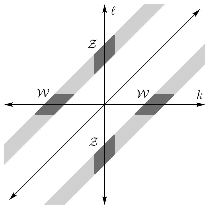
Since each of the aforementioned regions will be dealt with differently, we define the regions
𝒲 = { ( k , ℓ ) ∈ supp ( G ^ c ( k − ℓ ) ) | | ℓ | < δ } , 𝒲 conditional-set 𝑘 ℓ supp superscript ^ 𝐺 𝑐 𝑘 ℓ ℓ 𝛿 \mathcal{W}=\left\{(k,\ell)\in\text{supp}(\widehat{G}^{c}(k-\ell))\;\big{|}\;|\ell|<\delta\right\},
𝒵 = { ( k , ℓ ) ∈ supp ( G ^ c ( k − ℓ ) ) | | k | < δ } , 𝒵 conditional-set 𝑘 ℓ supp superscript ^ 𝐺 𝑐 𝑘 ℓ 𝑘 𝛿 \mathcal{Z}=\left\{(k,\ell)\in\text{supp}(\widehat{G}^{c}(k-\ell))\;\big{|}\;|k|<\delta\right\},
and
𝒱 = supp ( G ^ c ( k − ℓ ) ) \ ( 𝒲 ∪ 𝒵 ) . 𝒱 \ supp superscript ^ 𝐺 𝑐 𝑘 ℓ 𝒲 𝒵 \mathcal{V}=\text{supp}(\widehat{G}^{c}(k-\ell))\backslash(\mathcal{W}\cup\mathcal{Z}).
These regions can all be seen in the plot below.
Figure 1: Partition of k ℓ 𝑘 ℓ k\ell
We now bound each region separately.
5.2 In the region 𝒱 𝒱 \mathcal{V}
Over the region 𝒱 𝒱 \mathcal{V} ϑ ^ − 1 ( k ) = ϑ ^ ( ℓ ) = 1 . superscript ^ italic-ϑ 1 𝑘 ^ italic-ϑ ℓ 1 \widehat{\vartheta}^{-1}(k)=\widehat{\vartheta}(\ell)=1. 12 F , 𝐹 F, t 𝑡 t 9
ϵ ∑ j , m , n = 1 2 ∫ 0 t ∬ 𝒱 a ^ ( k , k − ℓ , ℓ ) e i ϕ m n j ( k , ℓ ) s f ^ j ( k ) ¯ g ^ m c ( k − ℓ ) f ^ n ( ℓ ) 𝑑 ℓ 𝑑 k 𝑑 s italic-ϵ superscript subscript 𝑗 𝑚 𝑛
1 2 superscript subscript 0 𝑡 subscript double-integral 𝒱 ^ 𝑎 𝑘 𝑘 ℓ ℓ superscript 𝑒 𝑖 subscript superscript italic-ϕ 𝑗 𝑚 𝑛 𝑘 ℓ 𝑠 ¯ subscript ^ 𝑓 𝑗 𝑘 subscript superscript ^ 𝑔 𝑐 𝑚 𝑘 ℓ subscript ^ 𝑓 𝑛 ℓ differential-d ℓ differential-d 𝑘 differential-d 𝑠 \epsilon\sum_{j,m,n=1}^{2}\int_{0}^{t}\iint_{\mathcal{V}}\widehat{a}(k,k-\ell,\ell)e^{i\phi^{j}_{mn}(k,\ell)s}\overline{\widehat{f}_{j}(k)}\widehat{g}^{c}_{m}(k-\ell)\widehat{f}_{n}(\ell)d\ell dkds (14)
with the following kernel functions a ^ ( k , k − ℓ , ℓ ) ^ 𝑎 𝑘 𝑘 ℓ ℓ \widehat{a}(k,k-\ell,\ell) 12
i ω j ( k ) , 1 2 k 2 i ω m ( k − ℓ ) ℓ 2 , i ω j ( k ) k 2 ( k − ℓ ) 2 , and 2 i ω j ( k ) k 2 ( k − ℓ ) ℓ . 𝑖 subscript 𝜔 𝑗 𝑘 1 2 superscript 𝑘 2 𝑖 subscript 𝜔 𝑚 𝑘 ℓ superscript ℓ 2 𝑖 subscript 𝜔 𝑗 𝑘 superscript 𝑘 2 superscript 𝑘 ℓ 2 and 2 𝑖 subscript 𝜔 𝑗 𝑘 superscript 𝑘 2 𝑘 ℓ ℓ
i\omega_{j}(k),\;\frac{1}{2}k^{2}i\omega_{m}(k-\ell)\ell^{2},\;i\omega_{j}(k)k^{2}(k-\ell)^{2},\text{ and }\;2i\omega_{j}(k)k^{2}(k-\ell)\ell.
We note that there are similar complex conjugate terms that can be dealt with in the same manner.
We integrate by parts with respect to s 𝑠 s
ϵ ∑ j , m , n = 1 2 ∬ 𝒱 a ^ ( k , k − ℓ , ℓ ) i ϕ m n j ( k , ℓ ) e i ϕ m n j ( k , ℓ ) s f ^ j ( k ) ¯ g ^ m c ( k − ℓ ) f ^ n ( ℓ ) 𝑑 ℓ 𝑑 k | 0 t evaluated-at italic-ϵ superscript subscript 𝑗 𝑚 𝑛
1 2 subscript double-integral 𝒱 ^ 𝑎 𝑘 𝑘 ℓ ℓ 𝑖 subscript superscript italic-ϕ 𝑗 𝑚 𝑛 𝑘 ℓ superscript 𝑒 𝑖 subscript superscript italic-ϕ 𝑗 𝑚 𝑛 𝑘 ℓ 𝑠 ¯ subscript ^ 𝑓 𝑗 𝑘 subscript superscript ^ 𝑔 𝑐 𝑚 𝑘 ℓ subscript ^ 𝑓 𝑛 ℓ differential-d ℓ differential-d 𝑘 0 𝑡 \displaystyle\epsilon\sum_{j,m,n=1}^{2}\iint_{\mathcal{V}}\frac{\widehat{a}(k,k-\ell,\ell)}{i\phi^{j}_{mn}(k,\ell)}e^{i\phi^{j}_{mn}(k,\ell)s}\overline{\widehat{f}_{j}(k)}\widehat{g}^{c}_{m}(k-\ell)\widehat{f}_{n}(\ell)d\ell dk\bigg{|}_{0}^{t} (15)
− ϵ ∑ j , m , n = 1 2 ∫ 0 t ∬ 𝒱 a ^ ( k , k − ℓ , ℓ ) i ϕ m n j ( k , ℓ ) e i ϕ m n j ( k , ℓ ) s ∂ s ( f ^ j ( k ) ¯ g ^ m c ( k − ℓ ) f ^ n ( ℓ ) ) d ℓ d k d s . italic-ϵ superscript subscript 𝑗 𝑚 𝑛
1 2 superscript subscript 0 𝑡 subscript double-integral 𝒱 ^ 𝑎 𝑘 𝑘 ℓ ℓ 𝑖 subscript superscript italic-ϕ 𝑗 𝑚 𝑛 𝑘 ℓ superscript 𝑒 𝑖 subscript superscript italic-ϕ 𝑗 𝑚 𝑛 𝑘 ℓ 𝑠 subscript 𝑠 ¯ subscript ^ 𝑓 𝑗 𝑘 subscript superscript ^ 𝑔 𝑐 𝑚 𝑘 ℓ subscript ^ 𝑓 𝑛 ℓ 𝑑 ℓ 𝑑 𝑘 𝑑 𝑠 \displaystyle-\epsilon\sum_{j,m,n=1}^{2}\int_{0}^{t}\iint_{\mathcal{V}}\frac{\widehat{a}(k,k-\ell,\ell)}{i\phi^{j}_{mn}(k,\ell)}e^{i\phi^{j}_{mn}(k,\ell)s}\partial_{s}\left(\overline{\widehat{f}_{j}(k)}\widehat{g}^{c}_{m}(k-\ell)\widehat{f}_{n}(\ell)\right)d\ell dkds. (16)
Since 𝒯 ∩ 𝒱 = ∅ , 𝒯 𝒱 \mathcal{T}\cap\mathcal{V}=\emptyset, 15 C ϵ E . 𝐶 italic-ϵ 𝐸 C\epsilon E. C ϵ E , 𝐶 italic-ϵ 𝐸 C\epsilon E,
For (16
ϵ italic-ϵ \displaystyle\epsilon ∫ 0 t ∬ 𝒱 a ^ ( k , k − ℓ , ℓ ) i ϕ m n j ( k , ℓ ) e i ϕ m n j ( k , ℓ ) s ∂ s ( f ^ j ( k ) ¯ ) g ^ m c ( k − ℓ ) f ^ n ( ℓ ) d ℓ d k d s superscript subscript 0 𝑡 subscript double-integral 𝒱 ^ 𝑎 𝑘 𝑘 ℓ ℓ 𝑖 subscript superscript italic-ϕ 𝑗 𝑚 𝑛 𝑘 ℓ superscript 𝑒 𝑖 subscript superscript italic-ϕ 𝑗 𝑚 𝑛 𝑘 ℓ 𝑠 subscript 𝑠 ¯ subscript ^ 𝑓 𝑗 𝑘 subscript superscript ^ 𝑔 𝑐 𝑚 𝑘 ℓ subscript ^ 𝑓 𝑛 ℓ 𝑑 ℓ 𝑑 𝑘 𝑑 𝑠 \displaystyle\int_{0}^{t}\iint_{\mathcal{V}}\frac{\widehat{a}(k,k-\ell,\ell)}{i\phi^{j}_{mn}(k,\ell)}e^{i\phi^{j}_{mn}(k,\ell)s}\partial_{s}\left(\overline{\widehat{f}_{j}(k)}\right)\widehat{g}^{c}_{m}(k-\ell)\widehat{f}_{n}(\ell)d\ell dkds
= 2 ϵ 2 ∫ 0 t ∬ 𝒱 a ^ ( k , k − ℓ , ℓ ) i ϕ m n j ( k , ℓ ) e i ( ω m ( k − ℓ ) + ω n ( ℓ ) ) s 1 ϑ ^ ( k ) N ^ j ( e i Λ s g ^ , e i Λ s ϑ ^ f ^ ) ( k ) ¯ g ^ m c ( k − ℓ ) f ^ n ( ℓ ) 𝑑 ℓ 𝑑 k 𝑑 s absent 2 superscript italic-ϵ 2 superscript subscript 0 𝑡 subscript double-integral 𝒱 ^ 𝑎 𝑘 𝑘 ℓ ℓ 𝑖 subscript superscript italic-ϕ 𝑗 𝑚 𝑛 𝑘 ℓ superscript 𝑒 𝑖 subscript 𝜔 𝑚 𝑘 ℓ subscript 𝜔 𝑛 ℓ 𝑠 ¯ 1 ^ italic-ϑ 𝑘 subscript ^ 𝑁 𝑗 superscript 𝑒 𝑖 Λ 𝑠 ^ 𝑔 superscript 𝑒 𝑖 Λ 𝑠 ^ italic-ϑ ^ 𝑓 𝑘 subscript superscript ^ 𝑔 𝑐 𝑚 𝑘 ℓ subscript ^ 𝑓 𝑛 ℓ differential-d ℓ differential-d 𝑘 differential-d 𝑠 \displaystyle=2\epsilon^{2}\int_{0}^{t}\iint_{\mathcal{V}}\frac{\widehat{a}(k,k-\ell,\ell)}{i\phi^{j}_{mn}(k,\ell)}e^{i(\omega_{m}(k-\ell)+\omega_{n}(\ell))s}\overline{\frac{1}{\widehat{\vartheta}(k)}\widehat{N}_{j}(e^{i\Lambda s}\widehat{g},e^{i\Lambda s}\widehat{\vartheta}\widehat{f})(k)}\widehat{g}^{c}_{m}(k-\ell)\widehat{f}_{n}(\ell)d\ell dkds
+ ϵ β + 1 ∫ 0 t ∬ 𝒱 a ^ ( k , k − ℓ , ℓ ) i ϕ m n j ( k , ℓ ) e i ( ω m ( k − ℓ ) + ω n ( ℓ ) ) s 1 ϑ ^ ( k ) N ^ j ( e i Λ s ϑ ^ f ^ , e i Λ s ϑ ^ f ^ ) ( k ) ¯ g ^ m c ( k − ℓ ) f ^ n ( ℓ ) 𝑑 ℓ 𝑑 k 𝑑 s superscript italic-ϵ 𝛽 1 superscript subscript 0 𝑡 subscript double-integral 𝒱 ^ 𝑎 𝑘 𝑘 ℓ ℓ 𝑖 subscript superscript italic-ϕ 𝑗 𝑚 𝑛 𝑘 ℓ superscript 𝑒 𝑖 subscript 𝜔 𝑚 𝑘 ℓ subscript 𝜔 𝑛 ℓ 𝑠 ¯ 1 ^ italic-ϑ 𝑘 subscript ^ 𝑁 𝑗 superscript 𝑒 𝑖 Λ 𝑠 ^ italic-ϑ ^ 𝑓 superscript 𝑒 𝑖 Λ 𝑠 ^ italic-ϑ ^ 𝑓 𝑘 subscript superscript ^ 𝑔 𝑐 𝑚 𝑘 ℓ subscript ^ 𝑓 𝑛 ℓ differential-d ℓ differential-d 𝑘 differential-d 𝑠 \displaystyle+\epsilon^{\beta+1}\int_{0}^{t}\iint_{\mathcal{V}}\frac{\widehat{a}(k,k-\ell,\ell)}{i\phi^{j}_{mn}(k,\ell)}e^{i(\omega_{m}(k-\ell)+\omega_{n}(\ell))s}\overline{\frac{1}{\widehat{\vartheta}(k)}\widehat{N}_{j}(e^{i\Lambda s}\widehat{\vartheta}\widehat{f},e^{i\Lambda s}\widehat{\vartheta}\widehat{f})(k)}\widehat{g}^{c}_{m}(k-\ell)\widehat{f}_{n}(\ell)d\ell dkds
+ ϵ 1 − β ∫ 0 t ∬ 𝒱 a ^ ( k , k − ℓ , ℓ ) i ϕ m n j ( k , ℓ ) e i ( ω m ( k − ℓ ) + ω n ( ℓ ) ) s e i ω j ( k ) s 1 ϑ ^ ( k ) Res ( ϵ G ^ ) ¯ g ^ m c ( k − ℓ ) f ^ n ( ℓ ) 𝑑 ℓ 𝑑 k 𝑑 s superscript italic-ϵ 1 𝛽 superscript subscript 0 𝑡 subscript double-integral 𝒱 ^ 𝑎 𝑘 𝑘 ℓ ℓ 𝑖 subscript superscript italic-ϕ 𝑗 𝑚 𝑛 𝑘 ℓ superscript 𝑒 𝑖 subscript 𝜔 𝑚 𝑘 ℓ subscript 𝜔 𝑛 ℓ 𝑠 ¯ superscript 𝑒 𝑖 subscript 𝜔 𝑗 𝑘 𝑠 1 ^ italic-ϑ 𝑘 Res italic-ϵ ^ 𝐺 subscript superscript ^ 𝑔 𝑐 𝑚 𝑘 ℓ subscript ^ 𝑓 𝑛 ℓ differential-d ℓ differential-d 𝑘 differential-d 𝑠 \displaystyle+\epsilon^{1-\beta}\int_{0}^{t}\iint_{\mathcal{V}}\frac{\widehat{a}(k,k-\ell,\ell)}{i\phi^{j}_{mn}(k,\ell)}e^{i(\omega_{m}(k-\ell)+\omega_{n}(\ell))s}\overline{e^{i\omega_{j}(k)s}\frac{1}{\widehat{\vartheta}(k)}\text{Res}(\epsilon\widehat{G})}\widehat{g}^{c}_{m}(k-\ell)\widehat{f}_{n}(\ell)d\ell dkds
= 2 ϵ 2 ∫ 0 t ∬ 𝒱 a ^ ( k , k − ℓ , ℓ ) i ϕ m n j ( k , ℓ ) N ^ j ( G ^ , ϑ ^ F ^ ) ( k ) ¯ G ^ m c ( k − ℓ ) F ^ n ( ℓ ) 𝑑 ℓ 𝑑 k 𝑑 s absent 2 superscript italic-ϵ 2 superscript subscript 0 𝑡 subscript double-integral 𝒱 ^ 𝑎 𝑘 𝑘 ℓ ℓ 𝑖 subscript superscript italic-ϕ 𝑗 𝑚 𝑛 𝑘 ℓ ¯ subscript ^ 𝑁 𝑗 ^ 𝐺 ^ italic-ϑ ^ 𝐹 𝑘 superscript subscript ^ 𝐺 𝑚 𝑐 𝑘 ℓ subscript ^ 𝐹 𝑛 ℓ differential-d ℓ differential-d 𝑘 differential-d 𝑠 \displaystyle=2\epsilon^{2}\int_{0}^{t}\iint_{\mathcal{V}}\frac{\widehat{a}(k,k-\ell,\ell)}{i\phi^{j}_{mn}(k,\ell)}\overline{\widehat{N}_{j}(\widehat{G},\widehat{\vartheta}\widehat{F})(k)}\widehat{G}_{m}^{c}(k-\ell)\widehat{F}_{n}(\ell)d\ell dkds (17)
+ ϵ β + 1 ∫ 0 t ∬ 𝒱 a ^ ( k , k − ℓ , ℓ ) i ϕ m n j ( k , ℓ ) N ^ j ( ϑ ^ F ^ , ϑ ^ F ^ ) ( k ) ¯ G ^ m c ( k − ℓ ) F ^ n ( ℓ ) 𝑑 ℓ 𝑑 k 𝑑 s superscript italic-ϵ 𝛽 1 superscript subscript 0 𝑡 subscript double-integral 𝒱 ^ 𝑎 𝑘 𝑘 ℓ ℓ 𝑖 subscript superscript italic-ϕ 𝑗 𝑚 𝑛 𝑘 ℓ ¯ subscript ^ 𝑁 𝑗 ^ italic-ϑ ^ 𝐹 ^ italic-ϑ ^ 𝐹 𝑘 superscript subscript ^ 𝐺 𝑚 𝑐 𝑘 ℓ subscript ^ 𝐹 𝑛 ℓ differential-d ℓ differential-d 𝑘 differential-d 𝑠 \displaystyle+\epsilon^{\beta+1}\int_{0}^{t}\iint_{\mathcal{V}}\frac{\widehat{a}(k,k-\ell,\ell)}{i\phi^{j}_{mn}(k,\ell)}\overline{\widehat{N}_{j}(\widehat{\vartheta}\widehat{F},\widehat{\vartheta}\widehat{F})(k)}\widehat{G}_{m}^{c}(k-\ell)\widehat{F}_{n}(\ell)d\ell dkds (18)
+ ϵ 1 − β ∫ 0 t ∬ 𝒱 a ^ ( k , k − ℓ , ℓ ) i ϕ m n j ( k , ℓ ) Res ( ϵ G ^ ) ¯ G ^ m c ( k − ℓ ) F ^ n ( ℓ ) 𝑑 ℓ 𝑑 k 𝑑 s superscript italic-ϵ 1 𝛽 superscript subscript 0 𝑡 subscript double-integral 𝒱 ^ 𝑎 𝑘 𝑘 ℓ ℓ 𝑖 subscript superscript italic-ϕ 𝑗 𝑚 𝑛 𝑘 ℓ ¯ Res italic-ϵ ^ 𝐺 superscript subscript ^ 𝐺 𝑚 𝑐 𝑘 ℓ subscript ^ 𝐹 𝑛 ℓ differential-d ℓ differential-d 𝑘 differential-d 𝑠 \displaystyle+\epsilon^{1-\beta}\int_{0}^{t}\iint_{\mathcal{V}}\frac{\widehat{a}(k,k-\ell,\ell)}{i\phi^{j}_{mn}(k,\ell)}\overline{\text{Res}(\epsilon\widehat{G})}\widehat{G}_{m}^{c}(k-\ell)\widehat{F}_{n}(\ell)d\ell dkds (19)
where we dropped the 1 / ϑ ^ ( k ) 1 ^ italic-ϑ 𝑘 1/\widehat{\vartheta}(k) 𝒱 𝒱 \mathcal{V} 1 . 1 1. 19 C ϵ 2 E 1 / 2 𝐶 superscript italic-ϵ 2 superscript 𝐸 1 2 C\epsilon^{2}E^{1/2} 17 18
2 8 k 2 i ω m ( k − ℓ ) ℓ 2 2 8 superscript 𝑘 2 𝑖 subscript 𝜔 𝑚 𝑘 ℓ superscript ℓ 2 \frac{\sqrt{2}}{8}k^{2}i\omega_{m}(k-\ell)\ell^{2}
can be bounded using integration by parts, which in this context is really writing k = ( k − ℓ ) + ℓ , 𝑘 𝑘 ℓ ℓ k=(k-\ell)+\ell,
∬ 𝒱 2 i ω j ( k ) k 2 ( k − ℓ ) ℓ i ϕ m n j ( k , ℓ ) N ^ j ( ϑ ^ F ^ , ϑ ^ F ^ ) ( k ) ¯ G ^ m c ( k − ℓ ) F ^ n ( ℓ ) 𝑑 ℓ 𝑑 k subscript double-integral 𝒱 2 𝑖 subscript 𝜔 𝑗 𝑘 superscript 𝑘 2 𝑘 ℓ ℓ 𝑖 subscript superscript italic-ϕ 𝑗 𝑚 𝑛 𝑘 ℓ ¯ subscript ^ 𝑁 𝑗 ^ italic-ϑ ^ 𝐹 ^ italic-ϑ ^ 𝐹 𝑘 superscript subscript ^ 𝐺 𝑚 𝑐 𝑘 ℓ subscript ^ 𝐹 𝑛 ℓ differential-d ℓ differential-d 𝑘 \displaystyle\iint_{\mathcal{V}}\frac{2i\omega_{j}(k)k^{2}(k-\ell)\ell}{i\phi^{j}_{mn}(k,\ell)}\overline{\widehat{N}_{j}(\widehat{\vartheta}\widehat{F},\widehat{\vartheta}\widehat{F})(k)}\widehat{G}_{m}^{c}(k-\ell)\widehat{F}_{n}(\ell)d\ell dk
= − ∭ ℝ × 𝒱 2 i ω j ( k ) ω j ( k ) k 2 ( k − ℓ ) ℓ i ϕ m n j ( k , ℓ ) ϑ ^ ( k − p ) F ^ ( k − p ) ϑ ^ ( p ) F ^ ( p ) ¯ G ^ m c ( k − ℓ ) F ^ n ( ℓ ) 𝑑 p 𝑑 ℓ 𝑑 k absent subscript triple-integral ℝ 𝒱 2 𝑖 subscript 𝜔 𝑗 𝑘 subscript 𝜔 𝑗 𝑘 superscript 𝑘 2 𝑘 ℓ ℓ 𝑖 subscript superscript italic-ϕ 𝑗 𝑚 𝑛 𝑘 ℓ ¯ ^ italic-ϑ 𝑘 𝑝 ^ 𝐹 𝑘 𝑝 ^ italic-ϑ 𝑝 ^ 𝐹 𝑝 superscript subscript ^ 𝐺 𝑚 𝑐 𝑘 ℓ subscript ^ 𝐹 𝑛 ℓ differential-d 𝑝 differential-d ℓ differential-d 𝑘 \displaystyle=-\iiint_{\mathbb{R}\times\mathcal{V}}\frac{\sqrt{2}i\omega_{j}(k)\omega_{j}(k)k^{2}(k-\ell)\ell}{i\phi^{j}_{mn}(k,\ell)}\overline{\widehat{\vartheta}(k-p)\widehat{F}(k-p)\widehat{\vartheta}(p)\widehat{F}(p)}\widehat{G}_{m}^{c}(k-\ell)\widehat{F}_{n}(\ell)dpd\ell dk
≤ C ∫ ( ∫ | k 2 F ^ ( k − p ) F ^ ( p ) | 𝑑 p ) ( ∫ | k ( k − ℓ ) G ^ m c ( k − ℓ ) ℓ F ^ n ( ℓ ) | 𝑑 ℓ ) 𝑑 k absent 𝐶 superscript 𝑘 2 ^ 𝐹 𝑘 𝑝 ^ 𝐹 𝑝 differential-d 𝑝 𝑘 𝑘 ℓ superscript subscript ^ 𝐺 𝑚 𝑐 𝑘 ℓ ℓ subscript ^ 𝐹 𝑛 ℓ differential-d ℓ differential-d 𝑘 \displaystyle\leq C\int\left(\int\left|k^{2}\widehat{F}(k-p)\widehat{F}(p)\right|dp\right)\left(\int\left|k(k-\ell)\widehat{G}_{m}^{c}(k-\ell)\ell\widehat{F}_{n}(\ell)\right|d\ell\right)dk
≤ C ∫ ( ∫ | ( 1 + ( k − p ) 2 + p 2 ) F ^ ( k − p ) F ^ ( p ) | 𝑑 p ) absent 𝐶 1 superscript 𝑘 𝑝 2 superscript 𝑝 2 ^ 𝐹 𝑘 𝑝 ^ 𝐹 𝑝 differential-d 𝑝 \displaystyle\leq C\int\left(\int\left|(1+(k-p)^{2}+p^{2})\widehat{F}(k-p)\widehat{F}(p)\right|dp\right)
× ( ∫ | ( 1 + ( k − ℓ ) + ℓ ) ( k − ℓ ) G ^ m c ( k − ℓ ) ℓ F ^ n ( ℓ ) | 𝑑 ℓ ) d k absent 1 𝑘 ℓ ℓ 𝑘 ℓ superscript subscript ^ 𝐺 𝑚 𝑐 𝑘 ℓ ℓ subscript ^ 𝐹 𝑛 ℓ differential-d ℓ 𝑑 𝑘 \displaystyle\hskip 144.54pt\times\left(\int\left|(1+(k-\ell)+\ell)(k-\ell)\widehat{G}_{m}^{c}(k-\ell)\ell\widehat{F}_{n}(\ell)\right|d\ell\right)dk
≤ C ‖ F ^ ‖ L 1 ‖ F ‖ H 2 2 absent 𝐶 subscript norm ^ 𝐹 superscript 𝐿 1 subscript superscript norm 𝐹 2 superscript 𝐻 2 \displaystyle\leq C\|\widehat{F}\|_{L^{1}}\|F\|^{2}_{H^{2}}
≤ C ‖ F ‖ H 2 3 ≲ E 3 / 2 . absent 𝐶 superscript subscript norm 𝐹 superscript 𝐻 2 3 less-than-or-similar-to superscript 𝐸 3 2 \displaystyle\leq C\|F\|_{H^{2}}^{3}\lesssim E^{3/2}.
The second to last step used Cauchy-Schwarz, Young’s inequality, and the fact that ‖ G ^ c ‖ L 1 ≤ C subscript norm superscript ^ 𝐺 𝑐 superscript 𝐿 1 𝐶 \|\widehat{G}^{c}\|_{L^{1}}\leq C ϵ . italic-ϵ \epsilon.
∥ F ^ ∥ L 1 ≤ C ∥ ( 1 + ( ⋅ ) F ^ ( ⋅ ) ∥ L 2 ≤ C E 1 / 2 . \|\widehat{F}\|_{L^{1}}\leq C\|(1+(\cdot)\widehat{F}(\cdot)\|_{L^{2}}\leq CE^{1/2}.
The final term with kernel function 2 / 8 k 2 i ω m ( k − ℓ ) ℓ 2 2 8 superscript 𝑘 2 𝑖 subscript 𝜔 𝑚 𝑘 ℓ superscript ℓ 2 \sqrt{2}/8k^{2}i\omega_{m}(k-\ell)\ell^{2} k 𝑘 k ℓ . ℓ \ell. k 𝑘 k ℓ ℓ \ell F . 𝐹 F. F 𝐹 F 5 / 2 5 2 5/2 F . 𝐹 F.
Therefore, for this last one we must take advantage of the form of (7 17
− 1 4 ϵ 2 ∑ j = 1 2 ∫ 0 t ∑ m , n = 1 2 ∬ 𝒱 i ω j ( k ) ⋅ ω m ( k − ℓ ) ϕ m n j ( k , ℓ ) G ^ m c ( k − ℓ ) ℓ 2 F ^ n ( ℓ ) 1 4 superscript italic-ϵ 2 superscript subscript 𝑗 1 2 superscript subscript 0 𝑡 superscript subscript 𝑚 𝑛
1 2 subscript double-integral 𝒱 ⋅ 𝑖 subscript 𝜔 𝑗 𝑘 subscript 𝜔 𝑚 𝑘 ℓ subscript superscript italic-ϕ 𝑗 𝑚 𝑛 𝑘 ℓ superscript subscript ^ 𝐺 𝑚 𝑐 𝑘 ℓ superscript ℓ 2 subscript ^ 𝐹 𝑛 ℓ \displaystyle-\frac{1}{4}\epsilon^{2}\sum_{j=1}^{2}\int_{0}^{t}\sum_{m,n=1}^{2}\iint_{\mathcal{V}}\frac{i\omega_{j}(k)\cdot\omega_{m}(k-\ell)}{\phi^{j}_{mn}(k,\ell)}\widehat{G}_{m}^{c}(k-\ell)\ell^{2}\widehat{F}_{n}(\ell)
× ( ∑ q , r = 1 2 ∫ k 2 G ^ q ( k − p ) ϑ ^ ( p ) F ^ r ( p ) 𝑑 p ) ¯ d ℓ d k d s . absent ¯ superscript subscript 𝑞 𝑟
1 2 superscript 𝑘 2 subscript ^ 𝐺 𝑞 𝑘 𝑝 ^ italic-ϑ 𝑝 subscript ^ 𝐹 𝑟 𝑝 differential-d 𝑝 𝑑 ℓ 𝑑 𝑘 𝑑 𝑠 \displaystyle\hskip 144.54pt\times\overline{\left(\sum_{q,r=1}^{2}\int k^{2}\widehat{G}_{q}(k-p)\widehat{\vartheta}(p)\widehat{F}_{r}(p)dp\right)}d\ell dkds.
For j ≠ n , 𝑗 𝑛 j\neq n, k − ℓ ≈ ± k 0 . 𝑘 ℓ plus-or-minus subscript 𝑘 0 k-\ell\approx\pm k_{0}.
| i ω j ( k ) ⋅ ω m ( k − ℓ ) ϕ m n j ( k , ℓ ) − i ω m ( k − ℓ ) | ≤ C ⋅ 𝑖 subscript 𝜔 𝑗 𝑘 subscript 𝜔 𝑚 𝑘 ℓ subscript superscript italic-ϕ 𝑗 𝑚 𝑛 𝑘 ℓ 𝑖 subscript 𝜔 𝑚 𝑘 ℓ 𝐶 \left|\frac{i\omega_{j}(k)\cdot\omega_{m}(k-\ell)}{\phi^{j}_{mn}(k,\ell)}-i\omega_{m}(k-\ell)\right|\leq C
for all ( k , ℓ ) ∈ 𝒱 . 𝑘 ℓ 𝒱 (k,\ell)\in\mathcal{V}. j = n , 𝑗 𝑛 j=n,
| i ω j ( k ) ⋅ ω m ( k − ℓ ) ϕ m n j ( k , ℓ ) + i ω j ( k ) | ≤ C ⋅ 𝑖 subscript 𝜔 𝑗 𝑘 subscript 𝜔 𝑚 𝑘 ℓ subscript superscript italic-ϕ 𝑗 𝑚 𝑛 𝑘 ℓ 𝑖 subscript 𝜔 𝑗 𝑘 𝐶 \left|\frac{i\omega_{j}(k)\cdot\omega_{m}(k-\ell)}{\phi^{j}_{mn}(k,\ell)}+i\omega_{j}(k)\right|\leq C
for all ( k , ℓ ) ∈ 𝒱 . 𝑘 ℓ 𝒱 (k,\ell)\in\mathcal{V}. [8 ] . We can drop ϑ ^ ( p ) ^ italic-ϑ 𝑝 \widehat{\vartheta}(p) p 𝑝 p ℝ 2 superscript ℝ 2 \mathbb{R}^{2} 𝒱 𝒱 \mathcal{V} F 𝐹 F G 𝐺 G
1 4 ϵ 2 1 4 superscript italic-ϵ 2 \displaystyle\frac{1}{4}\epsilon^{2} ∫ 0 t ∫ ( ∑ j , m = 1 2 ∫ i ω j ( k ) G ^ m c ( k − ℓ ) ℓ 2 F ^ j ( ℓ ) 𝑑 ℓ ) ( ∑ q , r = 1 2 ∫ k 2 G ^ q ( k − p ) F ^ r ( p ) 𝑑 p ) ¯ 𝑑 k 𝑑 s superscript subscript 0 𝑡 superscript subscript 𝑗 𝑚
1 2 𝑖 subscript 𝜔 𝑗 𝑘 superscript subscript ^ 𝐺 𝑚 𝑐 𝑘 ℓ superscript ℓ 2 subscript ^ 𝐹 𝑗 ℓ differential-d ℓ ¯ superscript subscript 𝑞 𝑟
1 2 superscript 𝑘 2 subscript ^ 𝐺 𝑞 𝑘 𝑝 subscript ^ 𝐹 𝑟 𝑝 differential-d 𝑝 differential-d 𝑘 differential-d 𝑠 \displaystyle\int_{0}^{t}\int\left(\sum_{j,m=1}^{2}\int i\omega_{j}(k)\widehat{G}_{m}^{c}(k-\ell)\ell^{2}\widehat{F}_{j}(\ell)d\ell\right)\overline{\left(\sum_{q,r=1}^{2}\int k^{2}\widehat{G}_{q}(k-p)\widehat{F}_{r}(p)dp\right)}dkds
= \displaystyle= 1 4 ϵ 2 ∫ 0 t ∫ ( ∑ j , m = 1 2 Ω j ( G m c ∂ x 2 F j ) ) ( ∂ x 2 ( ∑ q , r = 1 2 G q F r ) ) 𝑑 x 𝑑 s 1 4 superscript italic-ϵ 2 superscript subscript 0 𝑡 superscript subscript 𝑗 𝑚
1 2 subscript Ω 𝑗 superscript subscript 𝐺 𝑚 𝑐 superscript subscript 𝑥 2 subscript 𝐹 𝑗 superscript subscript 𝑥 2 superscript subscript 𝑞 𝑟
1 2 subscript 𝐺 𝑞 subscript 𝐹 𝑟 differential-d 𝑥 differential-d 𝑠 \displaystyle\frac{1}{4}\epsilon^{2}\int_{0}^{t}\int\left(\sum_{j,m=1}^{2}\Omega_{j}\left(G_{m}^{c}\partial_{x}^{2}F_{j}\right)\right)\left(\partial_{x}^{2}\left(\sum_{q,r=1}^{2}G_{q}F_{r}\right)\right)\;dxds
= \displaystyle= 1 4 ϵ 2 ∫ 0 t ∫ ( Ω 1 ( ( G 1 c + G 2 c ) ∂ x 2 F 1 ) + Ω 2 ( ( G 1 c + G 2 c ) ∂ x 2 F 2 ) ) ∂ x 2 ( ( G 1 + G 2 ) ( F 1 + F 2 ) ) d x d s 1 4 superscript italic-ϵ 2 superscript subscript 0 𝑡 subscript Ω 1 superscript subscript 𝐺 1 𝑐 superscript subscript 𝐺 2 𝑐 superscript subscript 𝑥 2 subscript 𝐹 1 subscript Ω 2 superscript subscript 𝐺 1 𝑐 superscript subscript 𝐺 2 𝑐 superscript subscript 𝑥 2 subscript 𝐹 2 superscript subscript 𝑥 2 subscript 𝐺 1 subscript 𝐺 2 subscript 𝐹 1 subscript 𝐹 2 𝑑 𝑥 𝑑 𝑠 \displaystyle\frac{1}{4}\epsilon^{2}\int_{0}^{t}\int\left(\Omega_{1}\left(\left(G_{1}^{c}+G_{2}^{c}\right)\partial_{x}^{2}F_{1}\right)+\Omega_{2}\left(\left(G_{1}^{c}+G_{2}^{c}\right)\partial_{x}^{2}F_{2}\right)\right)\partial_{x}^{2}\left(\left(G_{1}+G_{2}\right)\left(F_{1}+F_{2}\right)\right)dxds
= \displaystyle= 1 4 ϵ 2 ∫ 0 t ∫ Ω ( ∂ x 2 ( F 1 − F 2 ) ( G 1 c + G 2 c ) ) ∂ x 2 ( ( G 1 + G 2 ) ( F 1 + F 2 ) ) d x d s 1 4 superscript italic-ϵ 2 superscript subscript 0 𝑡 Ω superscript subscript 𝑥 2 subscript 𝐹 1 subscript 𝐹 2 superscript subscript 𝐺 1 𝑐 superscript subscript 𝐺 2 𝑐 superscript subscript 𝑥 2 subscript 𝐺 1 subscript 𝐺 2 subscript 𝐹 1 subscript 𝐹 2 𝑑 𝑥 𝑑 𝑠 \displaystyle\frac{1}{4}\epsilon^{2}\int_{0}^{t}\int\Omega\left(\partial_{x}^{2}\left(F_{1}-F_{2}\right)\left(G_{1}^{c}+G_{2}^{c}\right)\right)\partial_{x}^{2}\left(\left(G_{1}+G_{2}\right)\left(F_{1}+F_{2}\right)\right)\;dxds
= \displaystyle= ϵ 2 ∫ 0 t ∫ Ω ( ∂ x 2 R 2 ⋅ Ψ 1 c ) ∂ x 2 ( Ψ 1 ⋅ R 1 ) d x d s superscript italic-ϵ 2 superscript subscript 0 𝑡 Ω superscript subscript 𝑥 2 ⋅ subscript 𝑅 2 superscript subscript Ψ 1 𝑐 superscript subscript 𝑥 2 ⋅ subscript Ψ 1 subscript 𝑅 1 𝑑 𝑥 𝑑 𝑠 \displaystyle\epsilon^{2}\int_{0}^{t}\int\Omega\left(\partial_{x}^{2}R_{2}\cdot\Psi_{1}^{c}\right)\partial_{x}^{2}\left(\Psi_{1}\cdot R_{1}\right)\;dxds
= \displaystyle= ϵ 2 ∫ 0 t ∫ Ω ( ∂ x 2 R 2 ) ⋅ Ψ 1 c ⋅ Ψ 1 ⋅ ∂ x 2 R 1 d x d s superscript italic-ϵ 2 superscript subscript 0 𝑡 ⋅ Ω superscript subscript 𝑥 2 subscript 𝑅 2 superscript subscript Ψ 1 𝑐 subscript Ψ 1 superscript subscript 𝑥 2 subscript 𝑅 1 𝑑 𝑥 𝑑 𝑠 \displaystyle\epsilon^{2}\int_{0}^{t}\int\Omega\left(\partial_{x}^{2}R_{2}\right)\cdot\Psi_{1}^{c}\cdot\Psi_{1}\cdot\partial_{x}^{2}R_{1}\;dxds
+ ϵ 2 ∫ 0 t ∫ [ Ω , Ψ 1 c ] ∂ x 2 R 2 ⋅ Ψ 1 ⋅ ∂ x 2 R 1 d x d s superscript italic-ϵ 2 superscript subscript 0 𝑡 Ω superscript subscript Ψ 1 𝑐 superscript subscript 𝑥 2 ⋅ subscript 𝑅 2 subscript Ψ 1 superscript subscript 𝑥 2 subscript 𝑅 1 𝑑 𝑥 𝑑 𝑠 \displaystyle+\epsilon^{2}\int_{0}^{t}\int\left[\Omega\;,\;\Psi_{1}^{c}\right]\partial_{x}^{2}R_{2}\cdot\Psi_{1}\cdot\partial_{x}^{2}R_{1}\;dxds
+ ϵ 2 ∫ 0 t ∫ Ω ( ∂ x 2 R 2 ⋅ Ψ 1 c ) [ ∂ x 2 , Ψ 1 ] R 1 𝑑 x 𝑑 s superscript italic-ϵ 2 superscript subscript 0 𝑡 Ω superscript subscript 𝑥 2 ⋅ subscript 𝑅 2 superscript subscript Ψ 1 𝑐 superscript subscript 𝑥 2 subscript Ψ 1 subscript 𝑅 1 differential-d 𝑥 differential-d 𝑠 \displaystyle+\epsilon^{2}\int_{0}^{t}\int\Omega\left(\partial_{x}^{2}R_{2}\cdot\Psi_{1}^{c}\right)\left[\partial_{x}^{2}\;,\;\Psi_{1}\right]R_{1}\;dxds
The last two commutators can be estimated directly using Corollary 7 9 4
ϵ 2 superscript italic-ϵ 2 \displaystyle\epsilon^{2} ∫ 0 t ∫ Ω ( ∂ x 2 R 2 ) Ψ 1 c ⋅ Ψ 1 ⋅ ∂ x 2 R 1 d x d s superscript subscript 0 𝑡 ⋅ Ω superscript subscript 𝑥 2 subscript 𝑅 2 superscript subscript Ψ 1 𝑐 subscript Ψ 1 superscript subscript 𝑥 2 subscript 𝑅 1 𝑑 𝑥 𝑑 𝑠 \displaystyle\int_{0}^{t}\int\Omega\left(\partial_{x}^{2}R_{2}\right)\Psi_{1}^{c}\cdot\Psi_{1}\cdot\partial_{x}^{2}R_{1}\;dxds
= \displaystyle= ϵ 2 ∫ 0 t ∫ ∂ x 2 ( ∂ t R 1 − ϵ − β ϑ − 1 Res ( ϵ Ψ ) ) Ψ 1 c ⋅ Ψ 1 ⋅ ∂ x 2 R 1 d x d s superscript italic-ϵ 2 superscript subscript 0 𝑡 superscript subscript 𝑥 2 ⋅ subscript 𝑡 subscript 𝑅 1 superscript italic-ϵ 𝛽 superscript italic-ϑ 1 Res italic-ϵ Ψ superscript subscript Ψ 1 𝑐 subscript Ψ 1 superscript subscript 𝑥 2 subscript 𝑅 1 𝑑 𝑥 𝑑 𝑠 \displaystyle\epsilon^{2}\int_{0}^{t}\int\partial_{x}^{2}\left(\partial_{t}R_{1}-\epsilon^{-\beta}\vartheta^{-1}\text{Res}(\epsilon\Psi)\right)\Psi_{1}^{c}\cdot\Psi_{1}\cdot\partial_{x}^{2}R_{1}\;dxds
= \displaystyle= 1 2 ϵ 2 ∫ ( ∂ x 2 R 1 ) 2 ( Ψ 1 c Ψ 1 ) 𝑑 x | 0 t − 1 2 ϵ 2 ∫ 0 t ∫ ( ∂ x 2 R 1 ) 2 ∂ t ( Ψ 1 c Ψ 1 ) d x d s evaluated-at 1 2 superscript italic-ϵ 2 superscript superscript subscript 𝑥 2 subscript 𝑅 1 2 superscript subscript Ψ 1 𝑐 subscript Ψ 1 differential-d 𝑥 0 𝑡 1 2 superscript italic-ϵ 2 superscript subscript 0 𝑡 superscript superscript subscript 𝑥 2 subscript 𝑅 1 2 subscript 𝑡 superscript subscript Ψ 1 𝑐 subscript Ψ 1 𝑑 𝑥 𝑑 𝑠 \displaystyle\frac{1}{2}\epsilon^{2}\int\left(\partial_{x}^{2}R_{1}\right)^{2}\left(\Psi_{1}^{c}\Psi_{1}\right)\;dx\bigg{|}_{0}^{t}-\frac{1}{2}\epsilon^{2}\int_{0}^{t}\int\left(\partial_{x}^{2}R_{1}\right)^{2}\partial_{t}\left(\Psi_{1}^{c}\Psi_{1}\right)\;dxds
− ϵ 2 − β ∫ 0 t ∫ ∂ x 2 ϑ − 1 Res ( ϵ Ψ ) ⋅ Ψ 1 c ⋅ Ψ 1 ⋅ ∂ x 2 R 1 d x d s superscript italic-ϵ 2 𝛽 superscript subscript 0 𝑡 superscript subscript 𝑥 2 ⋅ superscript italic-ϑ 1 Res italic-ϵ Ψ superscript subscript Ψ 1 𝑐 subscript Ψ 1 superscript subscript 𝑥 2 subscript 𝑅 1 𝑑 𝑥 𝑑 𝑠 \displaystyle-\epsilon^{2-\beta}\int_{0}^{t}\int\partial_{x}^{2}\vartheta^{-1}\text{Res}(\epsilon\Psi)\cdot\Psi_{1}^{c}\cdot\Psi_{1}\cdot\partial_{x}^{2}R_{1}\;dxds
Now the first term can be treated as earlier boundary terms; we subtract it from the left-hand side of our estimate using the fact that it is both small and bounded independent of t . 𝑡 t. C ϵ 2 ( 1 + E ) 𝐶 superscript italic-ϵ 2 1 𝐸 C\epsilon^{2}(1+E) 18 17 G q subscript 𝐺 𝑞 G_{q} F q subscript 𝐹 𝑞 F_{q}
ϵ β + 1 superscript italic-ϵ 𝛽 1 \displaystyle\epsilon^{\beta+1} ∫ 0 t ∫ Ω ( ∂ x 2 R 2 ⋅ Ψ 1 c ) ∂ x 2 ( R 1 ⋅ R 1 ) d x d s superscript subscript 0 𝑡 Ω superscript subscript 𝑥 2 ⋅ subscript 𝑅 2 superscript subscript Ψ 1 𝑐 superscript subscript 𝑥 2 ⋅ subscript 𝑅 1 subscript 𝑅 1 𝑑 𝑥 𝑑 𝑠 \displaystyle\int_{0}^{t}\int\Omega\left(\partial_{x}^{2}R_{2}\cdot\Psi_{1}^{c}\right)\partial_{x}^{2}\left(R_{1}\cdot R_{1}\right)\;dxds
= \displaystyle= 2 ϵ β + 1 ∫ 0 t ∫ Ω ( ∂ x 2 R 2 ⋅ Ψ 1 c ) ( ∂ x 2 R 1 ⋅ R 1 + ( ∂ x R 1 ) 2 ) 𝑑 x 𝑑 s . 2 superscript italic-ϵ 𝛽 1 superscript subscript 0 𝑡 Ω superscript subscript 𝑥 2 ⋅ subscript 𝑅 2 superscript subscript Ψ 1 𝑐 superscript subscript 𝑥 2 ⋅ subscript 𝑅 1 subscript 𝑅 1 superscript subscript 𝑥 subscript 𝑅 1 2 differential-d 𝑥 differential-d 𝑠 \displaystyle 2\epsilon^{\beta+1}\int_{0}^{t}\int\Omega\left(\partial_{x}^{2}R_{2}\cdot\Psi_{1}^{c}\right)(\partial_{x}^{2}R_{1}\cdot R_{1}+(\partial_{x}R_{1})^{2})\;dxds.
The second term here can be bounded using the following
2 ϵ β + 1 2 superscript italic-ϵ 𝛽 1 \displaystyle 2\epsilon^{\beta+1} ∫ 0 t ∫ Ω ( ∂ x 2 R 2 ⋅ Ψ 1 c ) ( ∂ x R 1 ) 2 𝑑 x 𝑑 s superscript subscript 0 𝑡 Ω superscript subscript 𝑥 2 ⋅ subscript 𝑅 2 superscript subscript Ψ 1 𝑐 superscript subscript 𝑥 subscript 𝑅 1 2 differential-d 𝑥 differential-d 𝑠 \displaystyle\int_{0}^{t}\int\Omega\left(\partial_{x}^{2}R_{2}\cdot\Psi_{1}^{c}\right)(\partial_{x}R_{1})^{2}\;dxds
= \displaystyle= − 2 ϵ β + 1 ∫ 0 t ∫ ( ∂ x 2 R 2 ⋅ Ψ 1 c ) Ω ( ( ∂ x R 1 ) 2 ) 𝑑 x 𝑑 s 2 superscript italic-ϵ 𝛽 1 superscript subscript 0 𝑡 superscript subscript 𝑥 2 ⋅ subscript 𝑅 2 superscript subscript Ψ 1 𝑐 Ω superscript subscript 𝑥 subscript 𝑅 1 2 differential-d 𝑥 differential-d 𝑠 \displaystyle-2\epsilon^{\beta+1}\int_{0}^{t}\int\left(\partial_{x}^{2}R_{2}\cdot\Psi_{1}^{c}\right)\Omega\left((\partial_{x}R_{1})^{2}\right)\;dxds
≤ \displaystyle\leq C ϵ β + 1 ∫ 0 t ‖ R 2 ‖ H 2 ‖ ( ∂ x R 1 ) 2 ‖ H 1 𝑑 s 𝐶 superscript italic-ϵ 𝛽 1 superscript subscript 0 𝑡 subscript norm subscript 𝑅 2 superscript 𝐻 2 subscript norm superscript subscript 𝑥 subscript 𝑅 1 2 superscript 𝐻 1 differential-d 𝑠 \displaystyle C\epsilon^{\beta+1}\int_{0}^{t}\|R_{2}\|_{H^{2}}\|(\partial_{x}R_{1})^{2}\|_{H^{1}}\;ds
≤ \displaystyle\leq C ϵ β + 1 ∫ 0 t ‖ R 2 ‖ H 2 ‖ R 1 ‖ H 2 2 𝑑 s 𝐶 superscript italic-ϵ 𝛽 1 superscript subscript 0 𝑡 subscript norm subscript 𝑅 2 superscript 𝐻 2 subscript superscript norm subscript 𝑅 1 2 superscript 𝐻 2 differential-d 𝑠 \displaystyle C\epsilon^{\beta+1}\int_{0}^{t}\|R_{2}\|_{H^{2}}\|R_{1}\|^{2}_{H^{2}}\;ds
≤ \displaystyle\leq C ϵ β + 1 ∫ 0 t E 3 / 2 𝑑 s 𝐶 superscript italic-ϵ 𝛽 1 superscript subscript 0 𝑡 superscript 𝐸 3 2 differential-d 𝑠 \displaystyle C\epsilon^{\beta+1}\int_{0}^{t}E^{3/2}\;ds
The first term can be bounded using similar commutator estimates from (17
2 ϵ β + 1 ∫ 0 t ∫ Ω ( ∂ x 2 R 2 ⋅ Ψ 1 c ) ∂ x 2 R 1 ⋅ R 1 d x d s 2 superscript italic-ϵ 𝛽 1 superscript subscript 0 𝑡 Ω superscript subscript 𝑥 2 ⋅ subscript 𝑅 2 superscript subscript Ψ 1 𝑐 superscript subscript 𝑥 2 ⋅ subscript 𝑅 1 subscript 𝑅 1 𝑑 𝑥 𝑑 𝑠 \displaystyle 2\epsilon^{\beta+1}\int_{0}^{t}\int\Omega\left(\partial_{x}^{2}R_{2}\cdot\Psi_{1}^{c}\right)\partial_{x}^{2}R_{1}\cdot R_{1}\;dxds
= 2 ϵ β + 1 ∫ 0 t ∫ Ω ( ∂ x 2 R 2 ) ⋅ Ψ 1 c ⋅ ∂ x 2 R 1 ⋅ R 1 d x d s + 2 ϵ β + 1 ∫ 0 t ∫ [ Ω , Ψ 1 c ] ∂ x 2 R 2 ⋅ ∂ x 2 R 1 ⋅ R 1 d x d s absent 2 superscript italic-ϵ 𝛽 1 superscript subscript 0 𝑡 ⋅ Ω superscript subscript 𝑥 2 subscript 𝑅 2 superscript subscript Ψ 1 𝑐 superscript subscript 𝑥 2 ⋅ subscript 𝑅 1 subscript 𝑅 1 𝑑 𝑥 𝑑 𝑠 2 superscript italic-ϵ 𝛽 1 superscript subscript 0 𝑡 Ω superscript subscript Ψ 1 𝑐 superscript subscript 𝑥 2 ⋅ subscript 𝑅 2 superscript subscript 𝑥 2 ⋅ subscript 𝑅 1 subscript 𝑅 1 𝑑 𝑥 𝑑 𝑠 \displaystyle=2\epsilon^{\beta+1}\int_{0}^{t}\int\Omega\left(\partial_{x}^{2}R_{2}\right)\cdot\Psi_{1}^{c}\cdot\partial_{x}^{2}R_{1}\cdot R_{1}dxds+2\epsilon^{\beta+1}\int_{0}^{t}\int\left[\Omega\;,\;\Psi_{1}^{c}\right]\partial_{x}^{2}R_{2}\cdot\partial_{x}^{2}R_{1}\cdot R_{1}dxds
= 2 ϵ β + 1 ∫ 0 t ∫ ∂ x 2 ( ∂ t R 1 − ϵ − β ϑ − 1 Res ( ϵ Ψ ) ) ⋅ Ψ 1 c ⋅ ∂ x 2 R 1 ⋅ R 1 d x d s absent 2 superscript italic-ϵ 𝛽 1 superscript subscript 0 𝑡 superscript subscript 𝑥 2 ⋅ subscript 𝑡 subscript 𝑅 1 superscript italic-ϵ 𝛽 superscript italic-ϑ 1 Res italic-ϵ Ψ superscript subscript Ψ 1 𝑐 superscript subscript 𝑥 2 ⋅ subscript 𝑅 1 subscript 𝑅 1 𝑑 𝑥 𝑑 𝑠 \displaystyle=2\epsilon^{\beta+1}\int_{0}^{t}\int\partial_{x}^{2}\left(\partial_{t}R_{1}-\epsilon^{-\beta}\vartheta^{-1}\text{Res}(\epsilon\Psi)\right)\cdot\Psi_{1}^{c}\cdot\partial_{x}^{2}R_{1}\cdot R_{1}\;dxds
+ 2 ϵ β + 1 ∫ 0 t ∫ [ Ω , Ψ 1 c ] ∂ x 2 R 2 ⋅ ∂ x 2 R 1 ⋅ R 1 d x d s 2 superscript italic-ϵ 𝛽 1 superscript subscript 0 𝑡 Ω superscript subscript Ψ 1 𝑐 superscript subscript 𝑥 2 ⋅ subscript 𝑅 2 superscript subscript 𝑥 2 ⋅ subscript 𝑅 1 subscript 𝑅 1 𝑑 𝑥 𝑑 𝑠 \displaystyle\hskip 72.26999pt+2\epsilon^{\beta+1}\int_{0}^{t}\int\left[\Omega\;,\;\Psi_{1}^{c}\right]\partial_{x}^{2}R_{2}\cdot\partial_{x}^{2}R_{1}\cdot R_{1}\;dxds
= ϵ β + 1 ∫ ∂ x 2 R 1 2 ⋅ Ψ 1 c ⋅ R 1 d x | 0 t − ϵ β + 1 ∫ 0 t ∫ ∂ x 2 R 1 2 ⋅ ∂ t ( Ψ 1 c ⋅ R 1 ) d x d s absent evaluated-at superscript italic-ϵ 𝛽 1 superscript subscript 𝑥 2 ⋅ superscript subscript 𝑅 1 2 superscript subscript Ψ 1 𝑐 subscript 𝑅 1 𝑑 𝑥 0 𝑡 superscript italic-ϵ 𝛽 1 superscript subscript 0 𝑡 superscript subscript 𝑥 2 ⋅ superscript subscript 𝑅 1 2 subscript 𝑡 ⋅ superscript subscript Ψ 1 𝑐 subscript 𝑅 1 𝑑 𝑥 𝑑 𝑠 \displaystyle=\epsilon^{\beta+1}\int\partial_{x}^{2}R_{1}^{2}\cdot\Psi_{1}^{c}\cdot R_{1}\;dx\bigg{|}_{0}^{t}-\epsilon^{\beta+1}\int_{0}^{t}\int\partial_{x}^{2}R_{1}^{2}\cdot\partial_{t}\left(\Psi_{1}^{c}\cdot R_{1}\right)\;dxds
− 2 ϵ ∫ 0 t ∫ ϑ − 1 Res ( ϵ Ψ ) ⋅ Ψ 1 c ⋅ ∂ x 2 R 1 ⋅ R 1 d x d s + 2 ϵ β + 1 ∫ 0 t ∫ [ Ω , Ψ 1 c ] ∂ x 2 R 2 ⋅ ∂ x 2 R 1 ⋅ R 1 d x d s 2 italic-ϵ superscript subscript 0 𝑡 ⋅ superscript italic-ϑ 1 Res italic-ϵ Ψ superscript subscript Ψ 1 𝑐 superscript subscript 𝑥 2 ⋅ subscript 𝑅 1 subscript 𝑅 1 𝑑 𝑥 𝑑 𝑠 2 superscript italic-ϵ 𝛽 1 superscript subscript 0 𝑡 Ω superscript subscript Ψ 1 𝑐 superscript subscript 𝑥 2 ⋅ subscript 𝑅 2 superscript subscript 𝑥 2 ⋅ subscript 𝑅 1 subscript 𝑅 1 𝑑 𝑥 𝑑 𝑠 \displaystyle-2\epsilon\int_{0}^{t}\int\vartheta^{-1}\text{Res}(\epsilon\Psi)\cdot\Psi_{1}^{c}\cdot\partial_{x}^{2}R_{1}\cdot R_{1}dxds+2\epsilon^{\beta+1}\int_{0}^{t}\int\left[\Omega\;,\;\Psi_{1}^{c}\right]\partial_{x}^{2}R_{2}\cdot\partial_{x}^{2}R_{1}\cdot R_{1}dxds
Again we subtract the boundary term from the left-hand side, the commutator is estimated using Corollary 7
Thus, over the region 𝒱 𝒱 \mathcal{V}
∫ 0 t ∂ s E ( s ) d s ≲ ∫ 0 t ϵ 2 ( 1 + E ) + ϵ 3 E 2 d s . less-than-or-similar-to superscript subscript 0 𝑡 subscript 𝑠 𝐸 𝑠 𝑑 𝑠 superscript subscript 0 𝑡 superscript italic-ϵ 2 1 𝐸 superscript italic-ϵ 3 superscript 𝐸 2 𝑑 𝑠 \int_{0}^{t}\partial_{s}E(s)\;ds\lesssim\int_{0}^{t}\epsilon^{2}(1+E)+\epsilon^{3}E^{2}\;ds.
5.3 In the region with ℓ ℓ \ell 𝒲 𝒲 \mathcal{W}
Again we are hoping to bound the terms from (12 𝒲 . 𝒲 \mathcal{W}. ϑ ^ − 1 ( k ) = 1 superscript ^ italic-ϑ 1 𝑘 1 \widehat{\vartheta}^{-1}(k)=1 𝒲 . 𝒲 \mathcal{W}. ϑ ^ ( ℓ ) ^ italic-ϑ ℓ \widehat{\vartheta}(\ell) ϑ ^ ( ℓ ) , ^ italic-ϑ ℓ \widehat{\vartheta}(\ell), ϑ 0 = ϑ − ϵ . subscript italic-ϑ 0 italic-ϑ italic-ϵ \vartheta_{0}=\vartheta-\epsilon. ϑ 0 ( ℓ ) = 0 subscript italic-ϑ 0 ℓ 0 \vartheta_{0}(\ell)=0 ℓ = 0 . ℓ 0 \ell=0. ϵ 2 superscript italic-ϵ 2 \epsilon^{2} t 𝑡 t
ϵ ∑ j , m , n = 1 2 ∫ 0 t ∬ 𝒲 a ^ ( k , k − ℓ , ℓ ) e i ϕ m n j ( k , ℓ ) s f ^ j ( k ) ¯ g ^ m ( k − ℓ ) ϑ ^ 0 ( ℓ ) f ^ n ( ℓ ) 𝑑 ℓ 𝑑 k 𝑑 s italic-ϵ superscript subscript 𝑗 𝑚 𝑛
1 2 superscript subscript 0 𝑡 subscript double-integral 𝒲 ^ 𝑎 𝑘 𝑘 ℓ ℓ superscript 𝑒 𝑖 subscript superscript italic-ϕ 𝑗 𝑚 𝑛 𝑘 ℓ 𝑠 ¯ subscript ^ 𝑓 𝑗 𝑘 subscript ^ 𝑔 𝑚 𝑘 ℓ subscript ^ italic-ϑ 0 ℓ subscript ^ 𝑓 𝑛 ℓ differential-d ℓ differential-d 𝑘 differential-d 𝑠 \epsilon\sum_{j,m,n=1}^{2}\int_{0}^{t}\iint_{\mathcal{W}}\widehat{a}(k,k-\ell,\ell)e^{i\phi^{j}_{mn}(k,\ell)s}\overline{\widehat{f}_{j}(k)}\widehat{g}_{m}(k-\ell)\widehat{\vartheta}_{0}(\ell)\widehat{f}_{n}(\ell)d\ell dkds
Then when we integrate by parts with respect to s , 𝑠 s,
ϵ ∑ j , m , n = 1 2 ∬ 𝒲 a ^ ( k , k − ℓ , ℓ ) i ϕ m n j ( k , ℓ ) e i ϕ m n j ( k , ℓ ) s f ^ j ( k ) ¯ g ^ m c ( k − ℓ ) ϑ ^ 0 ( ℓ ) f ^ n ( ℓ ) 𝑑 ℓ 𝑑 k | 0 t evaluated-at italic-ϵ superscript subscript 𝑗 𝑚 𝑛
1 2 subscript double-integral 𝒲 ^ 𝑎 𝑘 𝑘 ℓ ℓ 𝑖 subscript superscript italic-ϕ 𝑗 𝑚 𝑛 𝑘 ℓ superscript 𝑒 𝑖 subscript superscript italic-ϕ 𝑗 𝑚 𝑛 𝑘 ℓ 𝑠 ¯ subscript ^ 𝑓 𝑗 𝑘 subscript superscript ^ 𝑔 𝑐 𝑚 𝑘 ℓ subscript ^ italic-ϑ 0 ℓ subscript ^ 𝑓 𝑛 ℓ differential-d ℓ differential-d 𝑘 0 𝑡 \displaystyle\epsilon\sum_{j,m,n=1}^{2}\iint_{\mathcal{W}}\frac{\widehat{a}(k,k-\ell,\ell)}{i\phi^{j}_{mn}(k,\ell)}e^{i\phi^{j}_{mn}(k,\ell)s}\overline{\widehat{f}_{j}(k)}\widehat{g}^{c}_{m}(k-\ell)\widehat{\vartheta}_{0}(\ell)\widehat{f}_{n}(\ell)d\ell dk\bigg{|}_{0}^{t} (20)
− ϵ ∑ j , m , n = 1 2 ∫ 0 t ∬ 𝒲 a ^ ( k , k − ℓ , ℓ ) i ϕ m n j ( k , ℓ ) e i ϕ m n j ( k , ℓ ) s ϑ ^ 0 ( ℓ ) ∂ s ( f ^ j ( k ) ¯ g ^ m c ( k − ℓ ) f ^ n ( ℓ ) ) d ℓ d k d s . italic-ϵ superscript subscript 𝑗 𝑚 𝑛
1 2 superscript subscript 0 𝑡 subscript double-integral 𝒲 ^ 𝑎 𝑘 𝑘 ℓ ℓ 𝑖 subscript superscript italic-ϕ 𝑗 𝑚 𝑛 𝑘 ℓ superscript 𝑒 𝑖 subscript superscript italic-ϕ 𝑗 𝑚 𝑛 𝑘 ℓ 𝑠 subscript ^ italic-ϑ 0 ℓ subscript 𝑠 ¯ subscript ^ 𝑓 𝑗 𝑘 subscript superscript ^ 𝑔 𝑐 𝑚 𝑘 ℓ subscript ^ 𝑓 𝑛 ℓ 𝑑 ℓ 𝑑 𝑘 𝑑 𝑠 \displaystyle-\epsilon\sum_{j,m,n=1}^{2}\int_{0}^{t}\iint_{\mathcal{W}}\frac{\widehat{a}(k,k-\ell,\ell)}{i\phi^{j}_{mn}(k,\ell)}e^{i\phi^{j}_{mn}(k,\ell)s}\widehat{\vartheta}_{0}(\ell)\partial_{s}\left(\overline{\widehat{f}_{j}(k)}\widehat{g}^{c}_{m}(k-\ell)\widehat{f}_{n}(\ell)\right)d\ell dkds. (21)
We note that 𝒯 ∩ 𝒲 = { ℓ = 0 } . 𝒯 𝒲 ℓ 0 \mathcal{T}\cap\mathcal{W}=\{\ell=0\}. ϑ ^ 0 ( 0 ) = 0 subscript ^ italic-ϑ 0 0 0 \widehat{\vartheta}_{0}(0)=0 ( k , ℓ ) ∈ 𝒲 , 𝑘 ℓ 𝒲 (k,\ell)\in\mathcal{W},
| a ^ ( k , k − ℓ , ℓ ) ϑ ^ 0 ( ℓ ) i ϕ m n j ( k , ℓ ) | < C . ^ 𝑎 𝑘 𝑘 ℓ ℓ subscript ^ italic-ϑ 0 ℓ 𝑖 subscript superscript italic-ϕ 𝑗 𝑚 𝑛 𝑘 ℓ 𝐶 \left|\frac{\widehat{a}(k,k-\ell,\ell)\widehat{\vartheta}_{0}(\ell)}{i\phi^{j}_{mn}(k,\ell)}\right|<C.
Therefore, the boundary term (20 ϵ E . italic-ϵ 𝐸 \epsilon E. 𝒱 . 𝒱 \mathcal{V}.
For the non-boundary term we can use the fact that 𝒲 𝒲 \mathcal{W} 𝒱 . 𝒱 \mathcal{V}.
Finally, for the two terms without ϑ ^ ( ℓ ) ^ italic-ϑ ℓ \widehat{\vartheta}(\ell) ℓ 2 superscript ℓ 2 \ell^{2}
| a ^ ( k , k − ℓ , ℓ ) i ϕ m n j ( k , ℓ ) | < C | ℓ | ^ 𝑎 𝑘 𝑘 ℓ ℓ 𝑖 subscript superscript italic-ϕ 𝑗 𝑚 𝑛 𝑘 ℓ 𝐶 ℓ \left|\frac{\widehat{a}(k,k-\ell,\ell)}{i\phi^{j}_{mn}(k,\ell)}\right|<C|\ell|
and so we can bound these terms directly after integrating by parts as well.
5.4 In the region with k 𝑘 k 𝒵 𝒵 \mathcal{Z}
Over the region 𝒵 𝒵 \mathcal{Z} 12 E 2 . subscript 𝐸 2 E_{2}. ϑ ^ − 1 ( k ) superscript ^ italic-ϑ 1 𝑘 \widehat{\vartheta}^{-1}(k) 𝒪 ( ϵ − 1 ) 𝒪 superscript italic-ϵ 1 \mathcal{O}(\epsilon^{-1}) k = 0 𝑘 0 k=0 𝒪 ( ϵ 3 ) 𝒪 superscript italic-ϵ 3 \mathcal{O}(\epsilon^{3}) ϵ 2 ( 1 + E ) + ϵ 3 E 2 . superscript italic-ϵ 2 1 𝐸 superscript italic-ϵ 3 superscript 𝐸 2 \epsilon^{2}(1+E)+\epsilon^{3}E^{2}. E 2 subscript 𝐸 2 E_{2} 𝒪 ( ϵ 2 E ) 𝒪 superscript italic-ϵ 2 𝐸 \mathcal{O}(\epsilon^{2}E) ϑ ^ ( ℓ ) = 1 ^ italic-ϑ ℓ 1 \widehat{\vartheta}(\ell)=1 𝒵 . 𝒵 \mathcal{Z}.
For 𝒪 ( ϵ ) 𝒪 italic-ϵ \mathcal{O}(\epsilon)
2 4 ϵ ∑ j , m , n = 1 2 ∬ 𝒵 ( i ω j ( k ) 1 ϑ ^ ( k ) + 1 2 k 2 i ω m ( k − ℓ ) ℓ 2 + i ω j ( k ) k 2 ( k − ℓ ) 2 1 ϑ ^ ( k ) \displaystyle\frac{\sqrt{2}}{4}\epsilon\sum^{2}_{j,m,n=1}\iint_{\mathcal{Z}}\bigg{(}i\omega_{j}(k)\frac{1}{\widehat{\vartheta}(k)}+\frac{1}{2}k^{2}i\omega_{m}(k-\ell)\ell^{2}+i\omega_{j}(k)k^{2}(k-\ell)^{2}\frac{1}{\widehat{\vartheta}(k)}
+ 2 i ω j ( k ) k 2 ( k − ℓ ) ℓ 1 ϑ ^ ( k ) + i ω j ( k ) k 2 ℓ 2 1 ϑ ^ ( k ) − i ω j ( k ) k 2 ℓ 2 ) F ^ j ( k ) ¯ G ^ m c ( k − ℓ ) F ^ n ( ℓ ) d ℓ d k \displaystyle\hskip 7.22743pt+2i\omega_{j}(k)k^{2}(k-\ell)\ell\frac{1}{\widehat{\vartheta}(k)}+i\omega_{j}(k)k^{2}\ell^{2}\frac{1}{\widehat{\vartheta}(k)}-i\omega_{j}(k)k^{2}\ell^{2}\bigg{)}\overline{\widehat{F}_{j}(k)}\widehat{G}_{m}^{c}(k-\ell)\widehat{F}_{n}(\ell)\;d\ell dk
+ 1 2 ∑ j = 1 2 ϵ ∫ | k | < δ Ω j F ^ j ¯ ⋅ B j ( G ^ c , F ^ ) + F ^ j ¯ ⋅ B j ( G ^ c , Λ F ^ ) + F ^ j ¯ ⋅ B j ( Λ G ^ c , F ^ ) 1 2 superscript subscript 𝑗 1 2 italic-ϵ subscript 𝑘 𝛿 ⋅ ¯ subscript Ω 𝑗 subscript ^ 𝐹 𝑗 subscript 𝐵 𝑗 superscript ^ 𝐺 𝑐 ^ 𝐹 ⋅ ¯ subscript ^ 𝐹 𝑗 subscript 𝐵 𝑗 superscript ^ 𝐺 𝑐 Λ ^ 𝐹 ⋅ ¯ subscript ^ 𝐹 𝑗 subscript 𝐵 𝑗 Λ superscript ^ 𝐺 𝑐 ^ 𝐹 \displaystyle+\frac{1}{2}\sum_{j=1}^{2}\epsilon\int\displaylimits_{|k|<\delta}\overline{\Omega_{j}\widehat{F}_{j}}\cdot B_{j}(\widehat{G}^{c},\widehat{F})+\overline{\widehat{F}_{j}}\cdot B_{j}(\widehat{G}^{c},\Lambda\widehat{F})+\overline{\widehat{F}_{j}}\cdot B_{j}(\Lambda\widehat{G}^{c},\widehat{F})
+ F ^ j ¯ ⋅ B j ( ( ∂ t − Λ ) G ^ c , F ^ ) d k ⋅ ¯ subscript ^ 𝐹 𝑗 subscript 𝐵 𝑗 subscript 𝑡 Λ superscript ^ 𝐺 𝑐 ^ 𝐹 𝑑 𝑘 \displaystyle\hskip 72.26999pt+\overline{\widehat{F}_{j}}\cdot B_{j}((\partial_{t}-\Lambda)\widehat{G}^{c},\widehat{F})\;dk
= 2 4 ϵ ∑ j , m , n = 1 2 ∬ 𝒵 ( 1 2 k 2 i ω m ( k − ℓ ) ℓ 2 + i ω j ( k ) k 2 ( k − ℓ ) 2 1 ϑ ^ ( k ) + 2 i ω j ( k ) k 2 ( k − ℓ ) ℓ 1 ϑ ^ ( k ) \displaystyle=\frac{\sqrt{2}}{4}\epsilon\sum^{2}_{j,m,n=1}\iint_{\mathcal{Z}}\bigg{(}\frac{1}{2}k^{2}i\omega_{m}(k-\ell)\ell^{2}+i\omega_{j}(k)k^{2}(k-\ell)^{2}\frac{1}{\widehat{\vartheta}(k)}+2i\omega_{j}(k)k^{2}(k-\ell)\ell\frac{1}{\widehat{\vartheta}(k)}
+ i ω j ( k ) k 2 ℓ 2 1 ϑ ^ ( k ) − i ω j ( k ) k 2 ℓ 2 ) F ^ j ( k ) ¯ G ^ m c ( k − ℓ ) F ^ n ( ℓ ) d ℓ d k \displaystyle\hskip 72.26999pt+i\omega_{j}(k)k^{2}\ell^{2}\frac{1}{\widehat{\vartheta}(k)}-i\omega_{j}(k)k^{2}\ell^{2}\bigg{)}\overline{\widehat{F}_{j}(k)}\widehat{G}_{m}^{c}(k-\ell)\widehat{F}_{n}(\ell)\;d\ell dk (22)
+ 1 2 ∑ j = 1 2 ϵ ∫ | k | < δ F ^ j ¯ ( 1 ϑ ^ ( k ) N j ( G ^ c , ϑ ^ F ^ ) − Ω j B j ( G ^ c , F ^ ) + B j ( G ^ c , Λ F ^ ) + B j ( Λ G ^ c , F ^ ) ) 𝑑 k 1 2 superscript subscript 𝑗 1 2 italic-ϵ subscript 𝑘 𝛿 ¯ subscript ^ 𝐹 𝑗 1 ^ italic-ϑ 𝑘 subscript 𝑁 𝑗 superscript ^ 𝐺 𝑐 ^ italic-ϑ ^ 𝐹 subscript Ω 𝑗 subscript 𝐵 𝑗 superscript ^ 𝐺 𝑐 ^ 𝐹 subscript 𝐵 𝑗 superscript ^ 𝐺 𝑐 Λ ^ 𝐹 subscript 𝐵 𝑗 Λ superscript ^ 𝐺 𝑐 ^ 𝐹 differential-d 𝑘 \displaystyle+\frac{1}{2}\sum_{j=1}^{2}\epsilon\int\displaylimits_{|k|<\delta}\overline{\widehat{F}_{j}}\bigg{(}\frac{1}{\widehat{\vartheta}(k)}N_{j}(\widehat{G}^{c},\widehat{\vartheta}\widehat{F})-\Omega_{j}B_{j}(\widehat{G}^{c},\widehat{F})+B_{j}(\widehat{G}^{c},\Lambda\widehat{F})+B_{j}(\Lambda\widehat{G}^{c},\widehat{F})\bigg{)}\;dk (23)
+ 1 2 ∑ j = 1 2 ϵ ∫ | k | < δ F ^ j ¯ ⋅ B j ( ( ∂ t − Λ ) G ^ c , F ^ ) 𝑑 k 1 2 superscript subscript 𝑗 1 2 italic-ϵ subscript 𝑘 𝛿 ⋅ ¯ subscript ^ 𝐹 𝑗 subscript 𝐵 𝑗 subscript 𝑡 Λ superscript ^ 𝐺 𝑐 ^ 𝐹 differential-d 𝑘 \displaystyle+\frac{1}{2}\sum_{j=1}^{2}\epsilon\int\displaylimits_{|k|<\delta}\overline{\widehat{F}_{j}}\cdot B_{j}((\partial_{t}-\Lambda)\widehat{G}^{c},\widehat{F})\;dk (24)
with similar complex conjugate terms. We will use space-time resonance methods on (22 E 2 subscript 𝐸 2 E_{2} 23 [14 ] , ‖ ( ∂ t − Λ ) G ^ c ‖ L 2 ≤ C ϵ 2 , subscript norm subscript 𝑡 Λ superscript ^ 𝐺 𝑐 superscript 𝐿 2 𝐶 superscript italic-ϵ 2 \|(\partial_{t}-\Lambda)\widehat{G}^{c}\|_{L^{2}}\leq C\epsilon^{2}, 24
For (22 t 𝑡 t
ϵ ∑ j , m , n = 1 2 ∫ 0 t ∬ 𝒵 a ^ ( k , k − ℓ , ℓ ) e i ϕ m n j ( k , ℓ ) s ϑ ^ − 1 ( k ) f ^ j ( k ) ¯ g ^ m c ( k − ℓ ) f ^ n ( ℓ ) 𝑑 ℓ 𝑑 k 𝑑 s italic-ϵ superscript subscript 𝑗 𝑚 𝑛
1 2 superscript subscript 0 𝑡 subscript double-integral 𝒵 ^ 𝑎 𝑘 𝑘 ℓ ℓ superscript 𝑒 𝑖 subscript superscript italic-ϕ 𝑗 𝑚 𝑛 𝑘 ℓ 𝑠 superscript ^ italic-ϑ 1 𝑘 ¯ subscript ^ 𝑓 𝑗 𝑘 subscript superscript ^ 𝑔 𝑐 𝑚 𝑘 ℓ subscript ^ 𝑓 𝑛 ℓ differential-d ℓ differential-d 𝑘 differential-d 𝑠 \epsilon\sum_{j,m,n=1}^{2}\int_{0}^{t}\iint_{\mathcal{Z}}\widehat{a}(k,k-\ell,\ell)e^{i\phi^{j}_{mn}(k,\ell)s}\widehat{\vartheta}^{-1}(k)\overline{\widehat{f}_{j}(k)}\widehat{g}^{c}_{m}(k-\ell)\widehat{f}_{n}(\ell)d\ell dkds
as well as two others without a factor of ϑ ^ − 1 ( k ) . superscript ^ italic-ϑ 1 𝑘 \widehat{\vartheta}^{-1}(k). s . 𝑠 s. ϑ ^ − 1 ( k ) superscript ^ italic-ϑ 1 𝑘 \widehat{\vartheta}^{-1}(k)
ϵ ∑ j , m , n = 1 2 ∬ 𝒵 a ^ ( k , k − ℓ , ℓ ) i ϕ m n j ( k , ℓ ) e i ϕ m n j ( k , ℓ ) s ϑ ^ − 1 ( k ) f ^ j ( k ) ¯ g ^ m c ( k − ℓ ) f ^ n ( ℓ ) 𝑑 ℓ 𝑑 k | 0 t evaluated-at italic-ϵ superscript subscript 𝑗 𝑚 𝑛
1 2 subscript double-integral 𝒵 ^ 𝑎 𝑘 𝑘 ℓ ℓ 𝑖 subscript superscript italic-ϕ 𝑗 𝑚 𝑛 𝑘 ℓ superscript 𝑒 𝑖 subscript superscript italic-ϕ 𝑗 𝑚 𝑛 𝑘 ℓ 𝑠 superscript ^ italic-ϑ 1 𝑘 ¯ subscript ^ 𝑓 𝑗 𝑘 subscript superscript ^ 𝑔 𝑐 𝑚 𝑘 ℓ subscript ^ 𝑓 𝑛 ℓ differential-d ℓ differential-d 𝑘 0 𝑡 \displaystyle\epsilon\sum_{j,m,n=1}^{2}\iint_{\mathcal{Z}}\frac{\widehat{a}(k,k-\ell,\ell)}{i\phi^{j}_{mn}(k,\ell)}e^{i\phi^{j}_{mn}(k,\ell)s}\widehat{\vartheta}^{-1}(k)\overline{\widehat{f}_{j}(k)}\widehat{g}^{c}_{m}(k-\ell)\widehat{f}_{n}(\ell)d\ell dk\bigg{|}_{0}^{t} (25)
− ϵ ∑ j , m , n = 1 2 ∫ 0 t ∬ 𝒵 a ^ ( k , k − ℓ , ℓ ) i ϕ m n j ( k , ℓ ) e i ϕ m n j ( k , ℓ ) s ϑ ^ − 1 ( k ) ∂ s ( f ^ j ( k ) ¯ g ^ m c ( k − ℓ ) f ^ n ( ℓ ) ) d ℓ d k d s . italic-ϵ superscript subscript 𝑗 𝑚 𝑛
1 2 superscript subscript 0 𝑡 subscript double-integral 𝒵 ^ 𝑎 𝑘 𝑘 ℓ ℓ 𝑖 subscript superscript italic-ϕ 𝑗 𝑚 𝑛 𝑘 ℓ superscript 𝑒 𝑖 subscript superscript italic-ϕ 𝑗 𝑚 𝑛 𝑘 ℓ 𝑠 superscript ^ italic-ϑ 1 𝑘 subscript 𝑠 ¯ subscript ^ 𝑓 𝑗 𝑘 subscript superscript ^ 𝑔 𝑐 𝑚 𝑘 ℓ subscript ^ 𝑓 𝑛 ℓ 𝑑 ℓ 𝑑 𝑘 𝑑 𝑠 \displaystyle-\epsilon\sum_{j,m,n=1}^{2}\int_{0}^{t}\iint_{\mathcal{Z}}\frac{\widehat{a}(k,k-\ell,\ell)}{i\phi^{j}_{mn}(k,\ell)}e^{i\phi^{j}_{mn}(k,\ell)s}\widehat{\vartheta}^{-1}(k)\partial_{s}\left(\overline{\widehat{f}_{j}(k)}\widehat{g}^{c}_{m}(k-\ell)\widehat{f}_{n}(\ell)\right)d\ell dkds. (26)
We note that 𝒯 ∩ 𝒵 = { k = 0 } . 𝒯 𝒵 𝑘 0 \mathcal{T}\cap\mathcal{Z}=\{k=0\}. a ^ ( 0 , − ℓ , ℓ ) = 0 ^ 𝑎 0 ℓ ℓ 0 \widehat{a}(0,-\ell,\ell)=0 0 0 ( k , ℓ ) ∈ 𝒵 , 𝑘 ℓ 𝒵 (k,\ell)\in\mathcal{Z},
| a ^ ( k , k − ℓ , ℓ ) i ϕ m n j ( k , ℓ ) | < C | k | 2 . ^ 𝑎 𝑘 𝑘 ℓ ℓ 𝑖 subscript superscript italic-ϕ 𝑗 𝑚 𝑛 𝑘 ℓ 𝐶 superscript 𝑘 2 \left|\frac{\widehat{a}(k,k-\ell,\ell)}{i\phi^{j}_{mn}(k,\ell)}\right|<C|k|^{2}.
Therefore, both terms are well-defined, and moreover, each of the kernel functions approach zero so rapidly we have
| a ^ ( k , k − ℓ , ℓ ) ϑ ^ − 1 ( k ) i ϕ m n j ( k , ℓ ) | < C | k | . ^ 𝑎 𝑘 𝑘 ℓ ℓ superscript ^ italic-ϑ 1 𝑘 𝑖 subscript superscript italic-ϕ 𝑗 𝑚 𝑛 𝑘 ℓ 𝐶 𝑘 \left|\frac{\widehat{a}(k,k-\ell,\ell)\widehat{\vartheta}^{-1}(k)}{i\phi^{j}_{mn}(k,\ell)}\right|<C|k|.
Therefore we use the fact that 𝒵 𝒵 \mathcal{Z} 𝒲 . 𝒲 \mathcal{W}. ϑ − 1 ( k ) superscript italic-ϑ 1 𝑘 \vartheta^{-1}(k)
| a ^ ( k , k − ℓ , ℓ ) i ϕ m n j ( k , ℓ ) | < C | k | ^ 𝑎 𝑘 𝑘 ℓ ℓ 𝑖 subscript superscript italic-ϕ 𝑗 𝑚 𝑛 𝑘 ℓ 𝐶 𝑘 \left|\frac{\widehat{a}(k,k-\ell,\ell)}{i\phi^{j}_{mn}(k,\ell)}\right|<C|k|
for ( k , ℓ ) ∈ 𝒵 . 𝑘 ℓ 𝒵 (k,\ell)\in\mathcal{Z}.
For the 𝒪 ( ϵ 2 ) 𝒪 superscript italic-ϵ 2 \mathcal{O}(\epsilon^{2}) 𝒵 𝒵 \mathcal{Z} G ^ c superscript ^ 𝐺 𝑐 \widehat{G}^{c} ‖ ( ∂ t − Λ ) G ^ c ‖ L 2 ≤ C ϵ 2 . subscript norm subscript 𝑡 Λ superscript ^ 𝐺 𝑐 superscript 𝐿 2 𝐶 superscript italic-ϵ 2 \|(\partial_{t}-\Lambda)\widehat{G}^{c}\|_{L^{2}}\leq C\epsilon^{2}.
ϵ 2 ∑ j = 1 2 superscript italic-ϵ 2 superscript subscript 𝑗 1 2 \displaystyle\epsilon^{2}\sum_{j=1}^{2} ∫ | k | < δ ( ϑ ^ − 1 N ^ j ( G ^ c , ϑ ^ F ^ ) + B j ( Λ G ^ c , F ^ ) + B j ( G ^ c , Λ F ^ ) ) ¯ ⋅ B j ( G ^ c , F ^ ) subscript 𝑘 𝛿 ⋅ ¯ superscript ^ italic-ϑ 1 subscript ^ 𝑁 𝑗 superscript ^ 𝐺 𝑐 ^ italic-ϑ ^ 𝐹 subscript 𝐵 𝑗 Λ superscript ^ 𝐺 𝑐 ^ 𝐹 subscript 𝐵 𝑗 superscript ^ 𝐺 𝑐 Λ ^ 𝐹 subscript 𝐵 𝑗 superscript ^ 𝐺 𝑐 ^ 𝐹 \displaystyle\int\displaylimits_{|k|<\delta}\overline{\left(\widehat{\vartheta}^{-1}\widehat{N}_{j}(\widehat{G}^{c},\widehat{\vartheta}\widehat{F})+B_{j}(\Lambda\widehat{G}^{c},\widehat{F})+B_{j}(\widehat{G}^{c},\Lambda\widehat{F})\right)}\cdot B_{j}(\widehat{G}^{c},\widehat{F})
+ F ^ j ¯ ⋅ B j ( G ^ c , ϑ ^ − 1 N ^ ( G ^ , ϑ F ^ ) ) d k + c . c . formulae-sequence ⋅ ¯ subscript ^ 𝐹 𝑗 subscript 𝐵 𝑗 superscript ^ 𝐺 𝑐 superscript ^ italic-ϑ 1 ^ 𝑁 ^ 𝐺 italic-ϑ ^ 𝐹 𝑑 𝑘 𝑐 𝑐 \displaystyle\hskip 36.135pt+\overline{\widehat{F}_{j}}\cdot B_{j}(\widehat{G}^{c},\widehat{\vartheta}^{-1}\widehat{N}(\widehat{G},\vartheta\widehat{F}))\;dk+c.c.
The first term and its complex conjugate can be written
ϵ 2 ∑ j = 1 2 ∫ | k | < δ ϑ ^ − 1 N ^ ( G ^ c , ϑ ^ F ^ ) ¯ ⋅ B j ( G ^ c , F ^ ) + ϑ ^ − 1 N ^ ( G ^ c , ϑ ^ F ^ ) ⋅ B j ( G ^ c , F ^ ) ¯ d k superscript italic-ϵ 2 superscript subscript 𝑗 1 2 subscript 𝑘 𝛿 ⋅ ¯ superscript ^ italic-ϑ 1 ^ 𝑁 superscript ^ 𝐺 𝑐 ^ italic-ϑ ^ 𝐹 subscript 𝐵 𝑗 superscript ^ 𝐺 𝑐 ^ 𝐹 ⋅ superscript ^ italic-ϑ 1 ^ 𝑁 superscript ^ 𝐺 𝑐 ^ italic-ϑ ^ 𝐹 ¯ subscript 𝐵 𝑗 superscript ^ 𝐺 𝑐 ^ 𝐹 𝑑 𝑘 \displaystyle\epsilon^{2}\sum_{j=1}^{2}\int\displaylimits_{|k|<\delta}\overline{\widehat{\vartheta}^{-1}\widehat{N}(\widehat{G}^{c},\widehat{\vartheta}\widehat{F})}\cdot B_{j}(\widehat{G}^{c},\widehat{F})+\widehat{\vartheta}^{-1}\widehat{N}(\widehat{G}^{c},\widehat{\vartheta}\widehat{F})\cdot\overline{B_{j}(\widehat{G}^{c},\widehat{F})}\;dk
= ϵ 2 ∑ j , m , n , q , r = 1 2 ∭ | k | < δ i ω j ( k ) 2 ϑ ^ ( p ) ϑ ^ ( k ) G ^ m c ( k − p ) F ^ n ( p ) ¯ ⋅ ω j ( k ) / 2 ϕ q r j ( k , ℓ ) ϑ ^ ( ℓ ) ϑ ^ ( k ) G ^ q c ( k − ℓ ) F ^ r ( ℓ ) absent superscript italic-ϵ 2 superscript subscript 𝑗 𝑚 𝑛
𝑞 𝑟
1
2 subscript triple-integral 𝑘 𝛿 ⋅ ¯ 𝑖 subscript 𝜔 𝑗 𝑘 2 ^ italic-ϑ 𝑝 ^ italic-ϑ 𝑘 superscript subscript ^ 𝐺 𝑚 𝑐 𝑘 𝑝 subscript ^ 𝐹 𝑛 𝑝 subscript 𝜔 𝑗 𝑘 2 subscript superscript italic-ϕ 𝑗 𝑞 𝑟 𝑘 ℓ ^ italic-ϑ ℓ ^ italic-ϑ 𝑘 subscript superscript ^ 𝐺 𝑐 𝑞 𝑘 ℓ subscript ^ 𝐹 𝑟 ℓ \displaystyle=\epsilon^{2}\sum_{\begin{subarray}{c}j,m,n,\\
q,r=1\end{subarray}}^{2}\iiint\displaylimits_{|k|<\delta}\overline{\frac{i\omega_{j}(k)}{\sqrt{2}}\frac{\widehat{\vartheta}(p)}{\widehat{\vartheta}(k)}\widehat{G}_{m}^{c}(k-p)\widehat{F}_{n}(p)}\cdot\frac{\omega_{j}(k)/\sqrt{2}}{\phi^{j}_{qr}(k,\ell)}\frac{\widehat{\vartheta}(\ell)}{\widehat{\vartheta}(k)}\widehat{G}^{c}_{q}(k-\ell)\widehat{F}_{r}(\ell)
+ i ω j ( k ) 2 ϑ ^ ( ℓ ) ϑ ^ ( k ) G ^ q c ( k − ℓ ) F ^ r ( ℓ ) ⋅ ω j ( k ) / 2 ϕ m n j ( k , p ) ϑ ( p ) ϑ ^ ( k ) G ^ m c ( k − p ) F ^ n ( p ) ¯ d p d ℓ d k ⋅ 𝑖 subscript 𝜔 𝑗 𝑘 2 ^ italic-ϑ ℓ ^ italic-ϑ 𝑘 subscript superscript ^ 𝐺 𝑐 𝑞 𝑘 ℓ subscript ^ 𝐹 𝑟 ℓ ¯ subscript 𝜔 𝑗 𝑘 2 subscript superscript italic-ϕ 𝑗 𝑚 𝑛 𝑘 𝑝 italic-ϑ 𝑝 ^ italic-ϑ 𝑘 superscript subscript ^ 𝐺 𝑚 𝑐 𝑘 𝑝 subscript ^ 𝐹 𝑛 𝑝 𝑑 𝑝 𝑑 ℓ 𝑑 𝑘 \displaystyle\hskip 72.26999pt+\frac{i\omega_{j}(k)}{\sqrt{2}}\frac{\widehat{\vartheta}(\ell)}{\widehat{\vartheta}(k)}\widehat{G}^{c}_{q}(k-\ell)\widehat{F}_{r}(\ell)\cdot\overline{\frac{\omega_{j}(k)/\sqrt{2}}{\phi^{j}_{mn}(k,p)}\frac{\vartheta(p)}{\widehat{\vartheta}(k)}\widehat{G}_{m}^{c}(k-p)\widehat{F}_{n}(p)}\;dpd\ell dk
= 1 2 ϵ 2 ∑ j , m , n , q , r = 1 2 ∭ | k | < δ i ω j ( k ) ω j ( k ) ϑ ^ ( p ) ϑ ^ ( ℓ ) ϑ ^ ( k ) ϑ ^ ( k ) ( − ω q ( k − ℓ ) − ω r ( ℓ ) + ω m ( k − p ) + ω n ( p ) ϕ m n j ( k , p ) ϕ q r j ( k , ℓ ) ) absent 1 2 superscript italic-ϵ 2 superscript subscript 𝑗 𝑚 𝑛
𝑞 𝑟
1
2 subscript triple-integral 𝑘 𝛿 𝑖 subscript 𝜔 𝑗 𝑘 subscript 𝜔 𝑗 𝑘 ^ italic-ϑ 𝑝 ^ italic-ϑ ℓ ^ italic-ϑ 𝑘 ^ italic-ϑ 𝑘 subscript 𝜔 𝑞 𝑘 ℓ subscript 𝜔 𝑟 ℓ subscript 𝜔 𝑚 𝑘 𝑝 subscript 𝜔 𝑛 𝑝 subscript superscript italic-ϕ 𝑗 𝑚 𝑛 𝑘 𝑝 subscript superscript italic-ϕ 𝑗 𝑞 𝑟 𝑘 ℓ \displaystyle=\frac{1}{2}\epsilon^{2}\sum_{\begin{subarray}{c}j,m,n,\\
q,r=1\end{subarray}}^{2}\iiint\displaylimits_{|k|<\delta}i\omega_{j}(k)\omega_{j}(k)\frac{\widehat{\vartheta}(p)\widehat{\vartheta}(\ell)}{\widehat{\vartheta}(k)\widehat{\vartheta}(k)}\left(\frac{-\omega_{q}(k-\ell)-\omega_{r}(\ell)+\omega_{m}(k-p)+\omega_{n}(p)}{\phi^{j}_{mn}(k,p)\phi^{j}_{qr}(k,\ell)}\right)
× G ^ m c ( k − p ) F ^ n ( p ) ¯ G ^ q c ( k − ℓ ) F ^ r ( ℓ ) d p d ℓ d k absent ¯ superscript subscript ^ 𝐺 𝑚 𝑐 𝑘 𝑝 subscript ^ 𝐹 𝑛 𝑝 subscript superscript ^ 𝐺 𝑐 𝑞 𝑘 ℓ subscript ^ 𝐹 𝑟 ℓ 𝑑 𝑝 𝑑 ℓ 𝑑 𝑘 \displaystyle\hskip 144.54pt\times\overline{\widehat{G}_{m}^{c}(k-p)\widehat{F}_{n}(p)}\widehat{G}^{c}_{q}(k-\ell)\widehat{F}_{r}(\ell)dpd\ell dk
The second and third term as well as their complex conjugates are
ϵ 2 ∑ j = 1 2 ∫ | k | < δ ( B j ( Λ G ^ c , F ^ ) + B j ( G ^ c , Λ F ^ ) ) ¯ B j ( G ^ c , F ^ ) + ( B j ( Λ G ^ c , F ^ ) + B j ( G ^ c , Λ F ^ ) ) B j ( G ^ c , F ^ ) ¯ d k superscript italic-ϵ 2 superscript subscript 𝑗 1 2 subscript 𝑘 𝛿 ¯ subscript 𝐵 𝑗 Λ superscript ^ 𝐺 𝑐 ^ 𝐹 subscript 𝐵 𝑗 superscript ^ 𝐺 𝑐 Λ ^ 𝐹 subscript 𝐵 𝑗 superscript ^ 𝐺 𝑐 ^ 𝐹 subscript 𝐵 𝑗 Λ superscript ^ 𝐺 𝑐 ^ 𝐹 subscript 𝐵 𝑗 superscript ^ 𝐺 𝑐 Λ ^ 𝐹 ¯ subscript 𝐵 𝑗 superscript ^ 𝐺 𝑐 ^ 𝐹 𝑑 𝑘 \displaystyle\epsilon^{2}\sum_{j=1}^{2}\int\displaylimits_{|k|<\delta}\overline{\big{(}B_{j}(\Lambda\widehat{G}^{c},\widehat{F})+B_{j}(\widehat{G}^{c},\Lambda\widehat{F})\big{)}}B_{j}(\widehat{G}^{c},\widehat{F})+\big{(}B_{j}(\Lambda\widehat{G}^{c},\widehat{F})+B_{j}(\widehat{G}^{c},\Lambda\widehat{F})\big{)}\overline{B_{j}(\widehat{G}^{c},\widehat{F})}dk
= \displaystyle= ϵ 2 ∑ j , m , n , q , r = 1 2 ∭ | k | < δ ω j ( k ) / 2 ϕ m n j ( k , p ) ϑ ^ ( p ) ϑ ^ ( k ) ( i ω m ( k − p ) + i ω n ( p ) ) G ^ m c ( k − p ) F ^ n ( p ) ¯ ω j ( k ) / 2 ϕ q r j ( k , ℓ ) ϑ ^ ( ℓ ) ϑ ^ ( k ) G ^ q c ( k − ℓ ) F ^ r ( ℓ ) superscript italic-ϵ 2 superscript subscript 𝑗 𝑚 𝑛
𝑞 𝑟
1
2 subscript triple-integral 𝑘 𝛿 ¯ subscript 𝜔 𝑗 𝑘 2 subscript superscript italic-ϕ 𝑗 𝑚 𝑛 𝑘 𝑝 ^ italic-ϑ 𝑝 ^ italic-ϑ 𝑘 𝑖 subscript 𝜔 𝑚 𝑘 𝑝 𝑖 subscript 𝜔 𝑛 𝑝 superscript subscript ^ 𝐺 𝑚 𝑐 𝑘 𝑝 subscript ^ 𝐹 𝑛 𝑝 subscript 𝜔 𝑗 𝑘 2 subscript superscript italic-ϕ 𝑗 𝑞 𝑟 𝑘 ℓ ^ italic-ϑ ℓ ^ italic-ϑ 𝑘 subscript superscript ^ 𝐺 𝑐 𝑞 𝑘 ℓ subscript ^ 𝐹 𝑟 ℓ \displaystyle\epsilon^{2}\sum_{\begin{subarray}{c}j,m,n,\\
q,r=1\end{subarray}}^{2}\iiint\displaylimits_{|k|<\delta}\overline{\frac{\omega_{j}(k)/\sqrt{2}}{\phi^{j}_{mn}(k,p)}\frac{\widehat{\vartheta}(p)}{\widehat{\vartheta}(k)}(i\omega_{m}(k-p)+i\omega_{n}(p))\widehat{G}_{m}^{c}(k-p)\widehat{F}_{n}(p)}\frac{\omega_{j}(k)/\sqrt{2}}{\phi^{j}_{qr}(k,\ell)}\frac{\widehat{\vartheta}(\ell)}{\widehat{\vartheta}(k)}\widehat{G}^{c}_{q}(k-\ell)\widehat{F}_{r}(\ell)
+ ω j ( k ) / 2 ϕ q r j ( k , ℓ ) ϑ ^ ( ℓ ) ϑ ^ ( k ) ( i ω q ( k − ℓ ) + i ω r ( ℓ ) ) G ^ q c ( k − ℓ ) F ^ r ( ℓ ) ⋅ ω j ( k ) / 2 ϕ m n j ( k , p ) ϑ ^ ( p ) ϑ ^ ( k ) G ^ m c ( k − p ) F ^ n ( p ) ¯ d ℓ d p d k ⋅ subscript 𝜔 𝑗 𝑘 2 subscript superscript italic-ϕ 𝑗 𝑞 𝑟 𝑘 ℓ ^ italic-ϑ ℓ ^ italic-ϑ 𝑘 𝑖 subscript 𝜔 𝑞 𝑘 ℓ 𝑖 subscript 𝜔 𝑟 ℓ subscript superscript ^ 𝐺 𝑐 𝑞 𝑘 ℓ subscript ^ 𝐹 𝑟 ℓ ¯ subscript 𝜔 𝑗 𝑘 2 subscript superscript italic-ϕ 𝑗 𝑚 𝑛 𝑘 𝑝 ^ italic-ϑ 𝑝 ^ italic-ϑ 𝑘 superscript subscript ^ 𝐺 𝑚 𝑐 𝑘 𝑝 subscript ^ 𝐹 𝑛 𝑝 𝑑 ℓ 𝑑 𝑝 𝑑 𝑘 \displaystyle+\frac{\omega_{j}(k)/\sqrt{2}}{\phi^{j}_{qr}(k,\ell)}\frac{\widehat{\vartheta}(\ell)}{\widehat{\vartheta}(k)}\left(i\omega_{q}(k-\ell)+i\omega_{r}(\ell)\right)\widehat{G}^{c}_{q}(k-\ell)\widehat{F}_{r}(\ell)\cdot\overline{\frac{\omega_{j}(k)/\sqrt{2}}{\phi^{j}_{mn}(k,p)}\frac{\widehat{\vartheta}(p)}{\widehat{\vartheta}(k)}\widehat{G}_{m}^{c}(k-p)\widehat{F}_{n}(p)}d\ell dpdk
= \displaystyle= − 1 2 ϵ 2 ∑ j , m , n , q , r = 1 2 ∭ | k | < δ i ω j ( k ) ω j ( k ) ϑ ^ ( p ) ϑ ^ ( ℓ ) ϑ ^ ( k ) ϑ ^ ( k ) ( − ω q ( k − ℓ ) − ω r ( ℓ ) + ω m ( k − p ) + ω n ( p ) ϕ m n j ( k , p ) ϕ q r j ( k , ℓ ) ) 1 2 superscript italic-ϵ 2 superscript subscript 𝑗 𝑚 𝑛
𝑞 𝑟
1
2 subscript triple-integral 𝑘 𝛿 𝑖 subscript 𝜔 𝑗 𝑘 subscript 𝜔 𝑗 𝑘 ^ italic-ϑ 𝑝 ^ italic-ϑ ℓ ^ italic-ϑ 𝑘 ^ italic-ϑ 𝑘 subscript 𝜔 𝑞 𝑘 ℓ subscript 𝜔 𝑟 ℓ subscript 𝜔 𝑚 𝑘 𝑝 subscript 𝜔 𝑛 𝑝 subscript superscript italic-ϕ 𝑗 𝑚 𝑛 𝑘 𝑝 subscript superscript italic-ϕ 𝑗 𝑞 𝑟 𝑘 ℓ \displaystyle-\frac{1}{2}\epsilon^{2}\sum_{\begin{subarray}{c}j,m,n,\\
q,r=1\end{subarray}}^{2}\iiint\displaylimits_{|k|<\delta}i\omega_{j}(k)\omega_{j}(k)\frac{\widehat{\vartheta}(p)\widehat{\vartheta}(\ell)}{\widehat{\vartheta}(k)\widehat{\vartheta}(k)}\left(\frac{-\omega_{q}(k-\ell)-\omega_{r}(\ell)+\omega_{m}(k-p)+\omega_{n}(p)}{\phi^{j}_{mn}(k,p)\phi^{j}_{qr}(k,\ell)}\right)
× G ^ m c ( k − p ) F ^ n ( p ) ¯ G ^ q c ( k − ℓ ) F ^ r ( ℓ ) d ℓ d p d k . absent ¯ superscript subscript ^ 𝐺 𝑚 𝑐 𝑘 𝑝 subscript ^ 𝐹 𝑛 𝑝 subscript superscript ^ 𝐺 𝑐 𝑞 𝑘 ℓ subscript ^ 𝐹 𝑟 ℓ 𝑑 ℓ 𝑑 𝑝 𝑑 𝑘 \displaystyle\hskip 144.54pt\times\overline{\widehat{G}_{m}^{c}(k-p)\widehat{F}_{n}(p)}\widehat{G}^{c}_{q}(k-\ell)\widehat{F}_{r}(\ell)d\ell dpdk.
These both cancel. The last term is of the form
ϵ 2 ∑ j = 1 2 ∫ | k | < δ F ^ j ¯ ⋅ B j ( G ^ c , ϑ ^ − 1 N ( G ^ , ϑ ^ F ^ ) ) 𝑑 k superscript italic-ϵ 2 superscript subscript 𝑗 1 2 subscript 𝑘 𝛿 ⋅ ¯ subscript ^ 𝐹 𝑗 subscript 𝐵 𝑗 superscript ^ 𝐺 𝑐 superscript ^ italic-ϑ 1 𝑁 ^ 𝐺 ^ italic-ϑ ^ 𝐹 differential-d 𝑘 \displaystyle\epsilon^{2}\sum_{j=1}^{2}\int\displaylimits_{|k|<\delta}\overline{\widehat{F}_{j}}\cdot B_{j}(\widehat{G}^{c},\widehat{\vartheta}^{-1}N(\widehat{G},\widehat{\vartheta}\widehat{F}))dk
= ϵ 2 ∑ j , m , n , q , r = 1 2 ∭ | k | < δ F ^ j ( k ) ¯ ⋅ ω j ( k ) / 2 ϕ m n j ( k , ℓ ) ϑ ^ ( ℓ ) ϑ ^ ( k ) G ^ m c ( k − ℓ ) ϑ ^ ( p ) ϑ ^ ( ℓ ) i ω n ( ℓ ) 2 G ^ q ( ℓ − p ) F ^ r ( p ) 𝑑 p 𝑑 ℓ 𝑑 k absent superscript italic-ϵ 2 superscript subscript 𝑗 𝑚 𝑛
𝑞 𝑟
1
2 subscript triple-integral 𝑘 𝛿 ⋅ ¯ subscript ^ 𝐹 𝑗 𝑘 subscript 𝜔 𝑗 𝑘 2 subscript superscript italic-ϕ 𝑗 𝑚 𝑛 𝑘 ℓ ^ italic-ϑ ℓ ^ italic-ϑ 𝑘 superscript subscript ^ 𝐺 𝑚 𝑐 𝑘 ℓ ^ italic-ϑ 𝑝 ^ italic-ϑ ℓ 𝑖 subscript 𝜔 𝑛 ℓ 2 subscript ^ 𝐺 𝑞 ℓ 𝑝 subscript ^ 𝐹 𝑟 𝑝 differential-d 𝑝 differential-d ℓ differential-d 𝑘 \displaystyle=\epsilon^{2}\sum_{\begin{subarray}{c}j,m,n,\\
q,r=1\end{subarray}}^{2}\iiint\displaylimits_{|k|<\delta}\overline{\widehat{F}_{j}(k)}\cdot\frac{\omega_{j}(k)/\sqrt{2}}{\phi^{j}_{mn}(k,\ell)}\frac{\widehat{\vartheta}(\ell)}{\widehat{\vartheta}(k)}\widehat{G}_{m}^{c}(k-\ell)\frac{\widehat{\vartheta}(p)}{\widehat{\vartheta}(\ell)}\frac{i\omega_{n}(\ell)}{\sqrt{2}}\widehat{G}_{q}(\ell-p)\widehat{F}_{r}(p)dpd\ell dk
= 1 2 ϵ 2 ∑ j , m , n , q , r = 1 2 ∭ | k | < δ i ω j ( k ) ω n ( ℓ ) ϕ m n j ( k , ℓ ) ϑ ^ ( p ) ϑ ^ ( k ) F ^ j ( k ) ¯ G ^ m c ( k − ℓ ) G ^ q ( ℓ − p ) F ^ r ( p ) 𝑑 p 𝑑 ℓ 𝑑 k absent 1 2 superscript italic-ϵ 2 superscript subscript 𝑗 𝑚 𝑛
𝑞 𝑟
1
2 subscript triple-integral 𝑘 𝛿 𝑖 subscript 𝜔 𝑗 𝑘 subscript 𝜔 𝑛 ℓ subscript superscript italic-ϕ 𝑗 𝑚 𝑛 𝑘 ℓ ^ italic-ϑ 𝑝 ^ italic-ϑ 𝑘 ¯ subscript ^ 𝐹 𝑗 𝑘 superscript subscript ^ 𝐺 𝑚 𝑐 𝑘 ℓ subscript ^ 𝐺 𝑞 ℓ 𝑝 subscript ^ 𝐹 𝑟 𝑝 differential-d 𝑝 differential-d ℓ differential-d 𝑘 \displaystyle=\frac{1}{2}\epsilon^{2}\sum_{\begin{subarray}{c}j,m,n,\\
q,r=1\end{subarray}}^{2}\iiint\displaylimits_{|k|<\delta}\frac{i\omega_{j}(k)\omega_{n}(\ell)}{\phi^{j}_{mn}(k,\ell)}\frac{\widehat{\vartheta}(p)}{\widehat{\vartheta}(k)}\overline{\widehat{F}_{j}(k)}\widehat{G}_{m}^{c}(k-\ell)\widehat{G}_{q}(\ell-p)\widehat{F}_{r}(p)dpd\ell dk
plus its complex conjugate. We can restrict to G ^ q c ( ℓ − p ) superscript subscript ^ 𝐺 𝑞 𝑐 ℓ 𝑝 \widehat{G}_{q}^{c}(\ell-p) G ^ q s superscript subscript ^ 𝐺 𝑞 𝑠 \widehat{G}_{q}^{s} 𝒪 ( ϵ 3 ) 𝒪 superscript italic-ϵ 3 \mathcal{O}(\epsilon^{3}) ϑ ^ − 1 ( k ) . superscript ^ italic-ϑ 1 𝑘 \widehat{\vartheta}^{-1}(k).
1 2 ϵ 2 ∑ j , m , n , q , r = 1 2 ∭ | k | < δ i ω j ( k ) ω n ( ℓ ) ϕ m n j ( k , ℓ ) ϑ ^ ( p ) ϑ ^ ( k ) F ^ j ( k ) ¯ G ^ m c ( k − ℓ ) G ^ q c ( ℓ − p ) F ^ r ( p ) 𝑑 p 𝑑 ℓ 𝑑 k . 1 2 superscript italic-ϵ 2 superscript subscript 𝑗 𝑚 𝑛
𝑞 𝑟
1
2 subscript triple-integral 𝑘 𝛿 𝑖 subscript 𝜔 𝑗 𝑘 subscript 𝜔 𝑛 ℓ subscript superscript italic-ϕ 𝑗 𝑚 𝑛 𝑘 ℓ ^ italic-ϑ 𝑝 ^ italic-ϑ 𝑘 ¯ subscript ^ 𝐹 𝑗 𝑘 superscript subscript ^ 𝐺 𝑚 𝑐 𝑘 ℓ subscript superscript ^ 𝐺 𝑐 𝑞 ℓ 𝑝 subscript ^ 𝐹 𝑟 𝑝 differential-d 𝑝 differential-d ℓ differential-d 𝑘 \frac{1}{2}\epsilon^{2}\sum_{\begin{subarray}{c}j,m,n,\\
q,r=1\end{subarray}}^{2}\iiint\displaylimits_{|k|<\delta}\frac{i\omega_{j}(k)\omega_{n}(\ell)}{\phi^{j}_{mn}(k,\ell)}\frac{\widehat{\vartheta}(p)}{\widehat{\vartheta}(k)}\overline{\widehat{F}_{j}(k)}\widehat{G}_{m}^{c}(k-\ell)\widehat{G}^{c}_{q}(\ell-p)\widehat{F}_{r}(p)dpd\ell dk. (27)
Using the support of G ^ c , superscript ^ 𝐺 𝑐 \widehat{G}^{c}, p 𝑝 p | k | < δ , 𝑘 𝛿 |k|<\delta, G ^ m c ( k − ℓ ) superscript subscript ^ 𝐺 𝑚 𝑐 𝑘 ℓ \widehat{G}_{m}^{c}(k-\ell) ℓ ≈ ± k 0 . ℓ plus-or-minus subscript 𝑘 0 \ell\approx\pm k_{0}. G ^ q c ( ℓ − p ) subscript superscript ^ 𝐺 𝑐 𝑞 ℓ 𝑝 \widehat{G}^{c}_{q}(\ell-p) p ≈ 0 𝑝 0 p\approx 0 p ≈ ± 2 k 0 . 𝑝 plus-or-minus 2 subscript 𝑘 0 p\approx\pm 2k_{0}.
G ^ c = ∑ { l = ± } G ^ c , l superscript ^ 𝐺 𝑐 subscript 𝑙 plus-or-minus superscript ^ 𝐺 𝑐 𝑙
\widehat{G}^{c}=\sum_{\{l=\pm\}}\widehat{G}^{c,l} (28)
with supp ( G ^ c , l ( k ) ) ⊂ { | k − l k 0 | < δ } supp superscript ^ 𝐺 𝑐 𝑙
𝑘 𝑘 𝑙 subscript 𝑘 0 𝛿 \text{supp}(\widehat{G}^{c,l}(k))\subset\{|k-lk_{0}|<\delta\}
ϵ 2 ∭ | k | < δ | p | < 3 δ i ω j ( k ) ω n ( ℓ ) ϕ m n j ( k , ℓ ) ϑ ^ ( p ) ϑ ^ ( k ) F ^ j ( k ) ¯ G ^ m c ( k − ℓ ) G ^ q c ( ℓ − p ) F ^ r ( p ) 𝑑 p 𝑑 ℓ 𝑑 k superscript italic-ϵ 2 subscript triple-integral 𝑘 𝛿 𝑝 3 𝛿
𝑖 subscript 𝜔 𝑗 𝑘 subscript 𝜔 𝑛 ℓ subscript superscript italic-ϕ 𝑗 𝑚 𝑛 𝑘 ℓ ^ italic-ϑ 𝑝 ^ italic-ϑ 𝑘 ¯ subscript ^ 𝐹 𝑗 𝑘 superscript subscript ^ 𝐺 𝑚 𝑐 𝑘 ℓ subscript superscript ^ 𝐺 𝑐 𝑞 ℓ 𝑝 subscript ^ 𝐹 𝑟 𝑝 differential-d 𝑝 differential-d ℓ differential-d 𝑘 \displaystyle\epsilon^{2}\iiint\displaylimits_{\begin{subarray}{c}|k|<\delta\\
|p|<3\delta\end{subarray}}\frac{i\omega_{j}(k)\omega_{n}(\ell)}{\phi^{j}_{mn}(k,\ell)}\frac{\widehat{\vartheta}(p)}{\widehat{\vartheta}(k)}\overline{\widehat{F}_{j}(k)}\widehat{G}_{m}^{c}(k-\ell)\widehat{G}^{c}_{q}(\ell-p)\widehat{F}_{r}(p)\;dpd\ell dk
= ϵ 2 ∫ ( ∫ | k | < δ i ω j ( k ) ω n ( ℓ ) ϕ m n j ( k , ℓ ) ϑ ^ ( k ) F ^ j ( k ) ¯ G ^ m c ( k − ℓ ) 𝑑 k ) absent superscript italic-ϵ 2 subscript 𝑘 𝛿 𝑖 subscript 𝜔 𝑗 𝑘 subscript 𝜔 𝑛 ℓ subscript superscript italic-ϕ 𝑗 𝑚 𝑛 𝑘 ℓ ^ italic-ϑ 𝑘 ¯ subscript ^ 𝐹 𝑗 𝑘 superscript subscript ^ 𝐺 𝑚 𝑐 𝑘 ℓ differential-d 𝑘 \displaystyle=\epsilon^{2}\int\bigg{(}\int\displaylimits_{|k|<\delta}\frac{i\omega_{j}(k)\omega_{n}(\ell)}{\phi^{j}_{mn}(k,\ell)\widehat{\vartheta}(k)}\overline{\widehat{F}_{j}(k)}\widehat{G}_{m}^{c}(k-\ell)dk\bigg{)}
× ( ∫ | p | < 3 δ ( ϑ ^ ( p ) − ϑ ^ ( ℓ − n k 0 ) ) G ^ q c , n ( ℓ − p ) F ^ r ( p ) 𝑑 p ) d ℓ absent subscript 𝑝 3 𝛿 ^ italic-ϑ 𝑝 ^ italic-ϑ ℓ 𝑛 subscript 𝑘 0 subscript superscript ^ 𝐺 𝑐 𝑛
𝑞 ℓ 𝑝 subscript ^ 𝐹 𝑟 𝑝 differential-d 𝑝 𝑑 ℓ \displaystyle\hskip 144.54pt\times\bigg{(}\int\displaylimits_{|p|<3\delta}(\widehat{\vartheta}(p)-\widehat{\vartheta}(\ell-nk_{0}))\widehat{G}^{c,n}_{q}(\ell-p)\widehat{F}_{r}(p)\;dp\bigg{)}d\ell
+ ϵ 2 ∫ ( ∫ | k | < δ i ω j ( k ) ω n ( ℓ ) ϕ m n j ( k , ℓ ) ϑ ^ ( k ) ( ϑ ^ ( ℓ − n k 0 ) − ϑ ^ ( k − ( l + n ) k 0 ) ) F ^ j ( k ) ¯ G ^ m c , l ( k − ℓ ) 𝑑 k ) superscript italic-ϵ 2 subscript 𝑘 𝛿 𝑖 subscript 𝜔 𝑗 𝑘 subscript 𝜔 𝑛 ℓ subscript superscript italic-ϕ 𝑗 𝑚 𝑛 𝑘 ℓ ^ italic-ϑ 𝑘 ^ italic-ϑ ℓ 𝑛 subscript 𝑘 0 ^ italic-ϑ 𝑘 𝑙 𝑛 subscript 𝑘 0 ¯ subscript ^ 𝐹 𝑗 𝑘 subscript superscript ^ 𝐺 𝑐 𝑙
𝑚 𝑘 ℓ differential-d 𝑘 \displaystyle+\epsilon^{2}\int\bigg{(}\int\displaylimits_{|k|<\delta}\frac{i\omega_{j}(k)\omega_{n}(\ell)}{\phi^{j}_{mn}(k,\ell)\widehat{\vartheta}(k)}\left(\widehat{\vartheta}(\ell-nk_{0})-\widehat{\vartheta}(k-(l+n)k_{0})\right)\overline{\widehat{F}_{j}(k)}\widehat{G}^{c,l}_{m}(k-\ell)dk\bigg{)}
× ( ∫ | p | < 3 δ G ^ q c , n ( ℓ − p ) F ^ r ( p ) 𝑑 p ) d ℓ absent subscript 𝑝 3 𝛿 subscript superscript ^ 𝐺 𝑐 𝑛
𝑞 ℓ 𝑝 subscript ^ 𝐹 𝑟 𝑝 differential-d 𝑝 𝑑 ℓ \displaystyle\hskip 144.54pt\times\bigg{(}\int\displaylimits_{|p|<3\delta}\widehat{G}^{c,n}_{q}(\ell-p)\widehat{F}_{r}(p)\;dp\bigg{)}d\ell
+ ϵ 2 ∫ ( ∫ | k | < δ i ω j ( k ) ω n ( ℓ ) ϕ m n j ( k , ℓ ) ϑ ^ ( k ) ϑ ^ ( k − ( l + n ) k 0 ) F ^ j ( k ) ¯ G ^ m c , l ( k − ℓ ) 𝑑 k ) superscript italic-ϵ 2 subscript 𝑘 𝛿 𝑖 subscript 𝜔 𝑗 𝑘 subscript 𝜔 𝑛 ℓ subscript superscript italic-ϕ 𝑗 𝑚 𝑛 𝑘 ℓ ^ italic-ϑ 𝑘 ^ italic-ϑ 𝑘 𝑙 𝑛 subscript 𝑘 0 ¯ subscript ^ 𝐹 𝑗 𝑘 subscript superscript ^ 𝐺 𝑐 𝑙
𝑚 𝑘 ℓ differential-d 𝑘 \displaystyle+\epsilon^{2}\int\bigg{(}\int\displaylimits_{|k|<\delta}\frac{i\omega_{j}(k)\omega_{n}(\ell)}{\phi^{j}_{mn}(k,\ell)\widehat{\vartheta}(k)}\widehat{\vartheta}(k-(l+n)k_{0})\overline{\widehat{F}_{j}(k)}\widehat{G}^{c,l}_{m}(k-\ell)dk\bigg{)}
× ( ∫ | p | < 3 δ G ^ q c , n ( ℓ − p ) F ^ r ( p ) 𝑑 p ) d ℓ absent subscript 𝑝 3 𝛿 subscript superscript ^ 𝐺 𝑐 𝑛
𝑞 ℓ 𝑝 subscript ^ 𝐹 𝑟 𝑝 differential-d 𝑝 𝑑 ℓ \displaystyle\hskip 144.54pt\times\bigg{(}\int\displaylimits_{|p|<3\delta}\widehat{G}^{c,n}_{q}(\ell-p)\widehat{F}_{r}(p)\;dp\bigg{)}d\ell
The first and second term can each be bounded using Proposition 12 l = − n 𝑙 𝑛 l=-n ϑ ^ ( k − ( l + n ) k 0 ) = ϑ ^ ( k ) . ^ italic-ϑ 𝑘 𝑙 𝑛 subscript 𝑘 0 ^ italic-ϑ 𝑘 \widehat{\vartheta}(k-(l+n)k_{0})=\widehat{\vartheta}(k). l = n , 𝑙 𝑛 l=n, t 𝑡 t E 1 . subscript 𝐸 1 E_{1}. [14 ] . We move to a rotating coordinate frame and we integrate with respect to t 𝑡 t
ϵ 2 ∑ j , m , n , q , r = 1 2 ∫ 0 t ∭ | k | < δ | p ± 2 k 0 | < 3 δ i ω j ( k ) ω n ( ℓ ) ϕ m n j ( k , ℓ ) ϑ ^ ( k ± 2 k 0 ) ϑ ^ ( k ) e i ϕ m q r j ( k , ℓ , p ) s f ^ j ( k ) ¯ g ^ m c ( k − ℓ ) g ^ q ( ℓ − p ) f ^ r ( p ) 𝑑 p 𝑑 ℓ 𝑑 k 𝑑 s superscript italic-ϵ 2 superscript subscript 𝑗 𝑚 𝑛
𝑞 𝑟
1
2 superscript subscript 0 𝑡 subscript triple-integral 𝑘 𝛿 plus-or-minus 𝑝 2 subscript 𝑘 0 3 𝛿
𝑖 subscript 𝜔 𝑗 𝑘 subscript 𝜔 𝑛 ℓ subscript superscript italic-ϕ 𝑗 𝑚 𝑛 𝑘 ℓ ^ italic-ϑ plus-or-minus 𝑘 2 subscript 𝑘 0 ^ italic-ϑ 𝑘 superscript 𝑒 𝑖 subscript superscript italic-ϕ 𝑗 𝑚 𝑞 𝑟 𝑘 ℓ 𝑝 𝑠 ¯ subscript ^ 𝑓 𝑗 𝑘 subscript superscript ^ 𝑔 𝑐 𝑚 𝑘 ℓ subscript ^ 𝑔 𝑞 ℓ 𝑝 subscript ^ 𝑓 𝑟 𝑝 differential-d 𝑝 differential-d ℓ differential-d 𝑘 differential-d 𝑠 \epsilon^{2}\sum_{\begin{subarray}{c}j,m,n,\\
q,r=1\end{subarray}}^{2}\int_{0}^{t}\iiint\displaylimits_{\begin{subarray}{c}|k|<\delta\\
|p\pm 2k_{0}|<3\delta\end{subarray}}\frac{i\omega_{j}(k)\omega_{n}(\ell)}{\phi^{j}_{mn}(k,\ell)}\frac{\widehat{\vartheta}(k\pm 2k_{0})}{\widehat{\vartheta}(k)}e^{i\phi^{j}_{mqr}(k,\ell,p)s}\overline{\widehat{f}_{j}(k)}\widehat{g}^{c}_{m}(k-\ell)\widehat{g}_{q}(\ell-p)\widehat{f}_{r}(p)\;dpd\ell dkds
with
ϕ m q r j ( k , ℓ , p ) = − ω j ( k ) + ω m ( k − ℓ ) + ω q ( ℓ − p ) + ω r ( p ) subscript superscript italic-ϕ 𝑗 𝑚 𝑞 𝑟 𝑘 ℓ 𝑝 subscript 𝜔 𝑗 𝑘 subscript 𝜔 𝑚 𝑘 ℓ subscript 𝜔 𝑞 ℓ 𝑝 subscript 𝜔 𝑟 𝑝 \phi^{j}_{mqr}(k,\ell,p)=-\omega_{j}(k)+\omega_{m}(k-\ell)+\omega_{q}(\ell-p)+\omega_{r}(p)
Since ϕ m q r j ( k , ℓ , p ) ≠ 0 subscript superscript italic-ϕ 𝑗 𝑚 𝑞 𝑟 𝑘 ℓ 𝑝 0 \phi^{j}_{mqr}(k,\ell,p)\neq 0 s 𝑠 s
ϵ 2 ∑ j , m , n , q , r = 1 2 ∫ 0 t ∭ i ω j ( k ) ω n ( ℓ ) i ϕ m n j ( k , ℓ ) ϕ m q r j ( k , ℓ , p ) ϑ ^ ( k ± 2 k 0 ) ϑ ^ ( k ) e i ϕ m q r j ( k , ℓ , p ) s superscript italic-ϵ 2 superscript subscript 𝑗 𝑚 𝑛
𝑞 𝑟
1
2 superscript subscript 0 𝑡 triple-integral 𝑖 subscript 𝜔 𝑗 𝑘 subscript 𝜔 𝑛 ℓ 𝑖 subscript superscript italic-ϕ 𝑗 𝑚 𝑛 𝑘 ℓ subscript superscript italic-ϕ 𝑗 𝑚 𝑞 𝑟 𝑘 ℓ 𝑝 ^ italic-ϑ plus-or-minus 𝑘 2 subscript 𝑘 0 ^ italic-ϑ 𝑘 superscript 𝑒 𝑖 subscript superscript italic-ϕ 𝑗 𝑚 𝑞 𝑟 𝑘 ℓ 𝑝 𝑠 \displaystyle\epsilon^{2}\sum_{\begin{subarray}{c}j,m,n,\\
q,r=1\end{subarray}}^{2}\int_{0}^{t}\iiint\frac{i\omega_{j}(k)\omega_{n}(\ell)}{i\phi^{j}_{mn}(k,\ell)\phi^{j}_{mqr}(k,\ell,p)}\frac{\widehat{\vartheta}(k\pm 2k_{0})}{\widehat{\vartheta}(k)}e^{i\phi^{j}_{mqr}(k,\ell,p)s}
× ∂ s ( f ^ j ( k ) ¯ g ^ m c ( k − ℓ ) g ^ q ( ℓ − p ) f ^ r ( p ) ) d p d ℓ d k d s \displaystyle\hskip 144.54pt\times\partial_{s}\left(\overline{\widehat{f}_{j}(k)}\widehat{g}^{c}_{m}(k-\ell)\widehat{g}_{q}(\ell-p)\widehat{f}_{r}(p)\right)\;dpd\ell dkds
plus a boundary term. Both can then be bounded directly.
For 𝒪 ( ϵ 3 ) 𝒪 superscript italic-ϵ 3 \mathcal{O}(\epsilon^{3})
2 ϵ 3 ∑ j = 1 2 ∫ | k | < δ B j ( G ^ c , ϑ ^ − 1 N ( G ^ , ϑ ^ F ^ ) ) ¯ ⋅ B j ( G ^ c , F ^ ) 2 superscript italic-ϵ 3 superscript subscript 𝑗 1 2 subscript 𝑘 𝛿 ⋅ ¯ subscript 𝐵 𝑗 superscript ^ 𝐺 𝑐 superscript ^ italic-ϑ 1 𝑁 ^ 𝐺 ^ italic-ϑ ^ 𝐹 subscript 𝐵 𝑗 superscript ^ 𝐺 𝑐 ^ 𝐹 \displaystyle 2\epsilon^{3}\sum_{j=1}^{2}\int\displaylimits_{|k|<\delta}\overline{B_{j}(\widehat{G}^{c},\widehat{\vartheta}^{-1}N(\widehat{G},\widehat{\vartheta}\widehat{F}))}\cdot B_{j}(\widehat{G}^{c},\widehat{F})
= 2 ϵ 3 ∑ j , m , n , q , r , a , b = 1 2 ⨌ | k | < δ ω j ( k ) / 2 ϕ m n j ( k , ℓ ) ϑ ^ ( ℓ ) ϑ ^ ( k ) G ^ m c ( k − ℓ ) ϑ ^ ( p ) ϑ ^ ( ℓ ) i ω n ( ℓ ) 2 G ^ q ( ℓ − p ) F ^ r ( p ) ¯ absent 2 superscript italic-ϵ 3 superscript subscript 𝑗 𝑚 𝑛 𝑞
𝑟 𝑎 𝑏
1
2 subscript quadruple-integral 𝑘 𝛿 ¯ subscript 𝜔 𝑗 𝑘 2 subscript superscript italic-ϕ 𝑗 𝑚 𝑛 𝑘 ℓ ^ italic-ϑ ℓ ^ italic-ϑ 𝑘 superscript subscript ^ 𝐺 𝑚 𝑐 𝑘 ℓ ^ italic-ϑ 𝑝 ^ italic-ϑ ℓ 𝑖 subscript 𝜔 𝑛 ℓ 2 subscript ^ 𝐺 𝑞 ℓ 𝑝 subscript ^ 𝐹 𝑟 𝑝 \displaystyle=2\epsilon^{3}\sum_{\begin{subarray}{c}j,m,n,q,\\
r,a,b=1\end{subarray}}^{2}\iiiint\displaylimits_{|k|<\delta}\overline{\frac{\omega_{j}(k)/\sqrt{2}}{\phi^{j}_{mn}(k,\ell)}\frac{\widehat{\vartheta}(\ell)}{\widehat{\vartheta}(k)}\widehat{G}_{m}^{c}(k-\ell)\frac{\widehat{\vartheta}(p)}{\widehat{\vartheta}(\ell)}\frac{i\omega_{n}(\ell)}{\sqrt{2}}\widehat{G}_{q}(\ell-p)\widehat{F}_{r}(p)}
× ω j ( k ) / 2 ϕ a b j ( k , q ) ϑ ^ ( q ) ϑ ^ ( k ) G ^ a c ( k − q ) F ^ b ( q ) d q d ℓ d p d k absent subscript 𝜔 𝑗 𝑘 2 subscript superscript italic-ϕ 𝑗 𝑎 𝑏 𝑘 𝑞 ^ italic-ϑ 𝑞 ^ italic-ϑ 𝑘 subscript superscript ^ 𝐺 𝑐 𝑎 𝑘 𝑞 subscript ^ 𝐹 𝑏 𝑞 𝑑 𝑞 𝑑 ℓ 𝑑 𝑝 𝑑 𝑘 \displaystyle\hskip 72.26999pt\times\frac{\omega_{j}(k)/\sqrt{2}}{\phi^{j}_{ab}(k,q)}\frac{\widehat{\vartheta}(q)}{\widehat{\vartheta}(k)}\widehat{G}^{c}_{a}(k-q)\widehat{F}_{b}(q)\;dqd\ell dpdk
along with the complex conjugate. Again we restrict to supp ( G ^ c ) supp superscript ^ 𝐺 𝑐 \text{supp}(\widehat{G}^{c})
− 2 2 ϵ 3 ∑ j , m , n , q , r , a , b = 1 2 2 2 superscript italic-ϵ 3 superscript subscript 𝑗 𝑚 𝑛 𝑞
𝑟 𝑎 𝑏
1
2 \displaystyle-\frac{\sqrt{2}}{2}\epsilon^{3}\sum_{\begin{subarray}{c}j,m,n,q,\\
r,a,b=1\end{subarray}}^{2} ⨌ | k | < δ i ω j ( k ) ω j ( k ) ω n ( ℓ ) ϕ m n j ( k , ℓ ) ϕ a b j ( k , q ) ϑ ^ ( p ) ϑ ^ ( q ) ϑ ^ ( k ) ϑ ^ ( k ) subscript quadruple-integral 𝑘 𝛿 𝑖 subscript 𝜔 𝑗 𝑘 subscript 𝜔 𝑗 𝑘 subscript 𝜔 𝑛 ℓ subscript superscript italic-ϕ 𝑗 𝑚 𝑛 𝑘 ℓ subscript superscript italic-ϕ 𝑗 𝑎 𝑏 𝑘 𝑞 ^ italic-ϑ 𝑝 ^ italic-ϑ 𝑞 ^ italic-ϑ 𝑘 ^ italic-ϑ 𝑘 \displaystyle\iiiint\displaylimits_{|k|<\delta}\frac{i\omega_{j}(k)\omega_{j}(k)\omega_{n}(\ell)}{\phi^{j}_{mn}(k,\ell)\phi^{j}_{ab}(k,q)}\frac{\widehat{\vartheta}(p)\widehat{\vartheta}(q)}{\widehat{\vartheta}(k)\widehat{\vartheta}(k)}
× G ^ m c ( k − ℓ ) G ^ q c ( ℓ − p ) F ^ r ( p ) ¯ G ^ a c ( k − q ) F ^ b ( q ) d q d ℓ d p d k absent ¯ superscript subscript ^ 𝐺 𝑚 𝑐 𝑘 ℓ subscript superscript ^ 𝐺 𝑐 𝑞 ℓ 𝑝 subscript ^ 𝐹 𝑟 𝑝 subscript superscript ^ 𝐺 𝑐 𝑎 𝑘 𝑞 subscript ^ 𝐹 𝑏 𝑞 𝑑 𝑞 𝑑 ℓ 𝑑 𝑝 𝑑 𝑘 \displaystyle\hskip 72.26999pt\times\overline{\widehat{G}_{m}^{c}(k-\ell)\widehat{G}^{c}_{q}(\ell-p)\widehat{F}_{r}(p)}\widehat{G}^{c}_{a}(k-q)\widehat{F}_{b}(q)\;dqd\ell dpdk
This term can be bounded exactly as (27 ℓ ℓ \ell p . 𝑝 p.
6 Error Estimates
In this section, we will put together the bounds found in each of the separate regions. Recall, that the goal is to show that the error is 𝒪 ( 1 ) 𝒪 1 \mathcal{O}(1) t ∈ [ 0 , T 0 ϵ 2 ] . 𝑡 0 subscript 𝑇 0 superscript italic-ϵ 2 t\in\left[0,\frac{T_{0}}{\epsilon^{2}}\right].
∂ t E ≲ ϵ 2 ( 1 + E ) + ϵ 3 E 2 less-than-or-similar-to subscript 𝑡 𝐸 superscript italic-ϵ 2 1 𝐸 superscript italic-ϵ 3 superscript 𝐸 2 \partial_{t}E\lesssim\epsilon^{2}(1+E)+\epsilon^{3}E^{2}
which by using Gronwall’s inequality will show
sup t ∈ [ 0 , T 0 / ϵ 2 ] E ( t ) ≤ C subscript supremum 𝑡 0 subscript 𝑇 0 superscript italic-ϵ 2 𝐸 𝑡 𝐶 \sup_{t\in[0,T_{0}/\epsilon^{2}]}E\left(t\right)\leq C
for a constant independent of ϵ . italic-ϵ \epsilon. E 1 , subscript 𝐸 1 E_{1}, ∂ t E subscript 𝑡 𝐸 \partial_{t}E ϵ italic-ϵ \epsilon E . 𝐸 E. t 𝑡 t
E ( t ) − E ( 0 ) = ∫ 0 t ∂ s E ( s ) d s . 𝐸 𝑡 𝐸 0 superscript subscript 0 𝑡 subscript 𝑠 𝐸 𝑠 𝑑 𝑠 E(t)-E(0)=\int_{0}^{t}\partial_{s}E(s)\;ds.
To bound the right-hand side we integrated by parts with respect to s 𝑠 s
E ( t ) − E ( 0 ) ≲ ϵ ( E ( t ) − E ( 0 ) ) + ∫ 0 t ϵ 2 ( 1 + E ( s ) ) + ϵ 3 E ( s ) 2 d s , less-than-or-similar-to 𝐸 𝑡 𝐸 0 italic-ϵ 𝐸 𝑡 𝐸 0 superscript subscript 0 𝑡 superscript italic-ϵ 2 1 𝐸 𝑠 superscript italic-ϵ 3 𝐸 superscript 𝑠 2 𝑑 𝑠 E(t)-E(0)\lesssim\epsilon\left(E(t)-E(0)\right)+\int_{0}^{t}\epsilon^{2}(1+E(s))+\epsilon^{3}E(s)^{2}\;ds,
and so
( 1 − C ϵ ) E ( t ) ≲ ( 1 − C ϵ ) E ( 0 ) + ∫ 0 t ϵ 2 ( 1 + E ( s ) ) + ϵ 3 E ( s ) 2 d s . less-than-or-similar-to 1 𝐶 italic-ϵ 𝐸 𝑡 1 𝐶 italic-ϵ 𝐸 0 superscript subscript 0 𝑡 superscript italic-ϵ 2 1 𝐸 𝑠 superscript italic-ϵ 3 𝐸 superscript 𝑠 2 𝑑 𝑠 (1-C\epsilon)E(t)\lesssim(1-C\epsilon)E(0)+\int_{0}^{t}\epsilon^{2}(1+E(s))+\epsilon^{3}E(s)^{2}\;ds.
In essence the boundary terms have been added to the energy as 𝒪 ( ϵ ) 𝒪 italic-ϵ \mathcal{O}(\epsilon) t , 𝑡 t, ‖ R ‖ H 2 . subscript norm 𝑅 superscript 𝐻 2 \|R\|_{H^{2}}.
E ( t ) ≤ C 1 ( E ( 0 ) + ∫ 0 t ϵ 2 ( 1 + E ( s ) ) + ϵ 3 E ( s ) 2 d s ) 𝐸 𝑡 subscript 𝐶 1 𝐸 0 superscript subscript 0 𝑡 superscript italic-ϵ 2 1 𝐸 𝑠 superscript italic-ϵ 3 𝐸 superscript 𝑠 2 𝑑 𝑠 E\left(t\right)\leq C_{1}\left(E(0)+\int_{0}^{t}\epsilon^{2}(1+E(s))+\epsilon^{3}E(s)^{2}\;ds\right)
and so for all t 𝑡 t ϵ E ( t ) ≤ 1 , italic-ϵ 𝐸 𝑡 1 \epsilon E(t)\leq 1,
E ( t ) 𝐸 𝑡 \displaystyle E\left(t\right) ≤ C 1 E ( 0 ) + C 1 ϵ 2 ∫ 0 t ( 1 + 2 E ( s ) ) 𝑑 s absent subscript 𝐶 1 𝐸 0 subscript 𝐶 1 superscript italic-ϵ 2 superscript subscript 0 𝑡 1 2 𝐸 𝑠 differential-d 𝑠 \displaystyle\leq C_{1}E(0)+C_{1}\epsilon^{2}\int_{0}^{t}(1+2E(s))\;ds
= C 1 ( E ( 0 ) + ϵ 2 t ) + 2 C 1 ϵ 2 ∫ 0 t E ( s ) 𝑑 s . absent subscript 𝐶 1 𝐸 0 superscript italic-ϵ 2 𝑡 2 subscript 𝐶 1 superscript italic-ϵ 2 superscript subscript 0 𝑡 𝐸 𝑠 differential-d 𝑠 \displaystyle=C_{1}(E(0)+\epsilon^{2}t)+2C_{1}\epsilon^{2}\int_{0}^{t}E(s)\;ds.
An application of Gronwall’s inequality then gives us
E ( t ) ≤ C 1 ( E ( 0 ) + ϵ 2 t ) e 2 C 1 ϵ 2 t . 𝐸 𝑡 subscript 𝐶 1 𝐸 0 superscript italic-ϵ 2 𝑡 superscript 𝑒 2 subscript 𝐶 1 superscript italic-ϵ 2 𝑡 E(t)\leq C_{1}\left(E(0)+\epsilon^{2}t\right)e^{2C_{1}\epsilon^{2}t}.
For t = T 0 / ϵ 2 𝑡 subscript 𝑇 0 superscript italic-ϵ 2 t=T_{0}/\epsilon^{2}
E ( T 0 / ϵ 2 ) ≤ C 1 ( E ( 0 ) + T 0 ) e 2 C 1 T 0 . 𝐸 subscript 𝑇 0 superscript italic-ϵ 2 subscript 𝐶 1 𝐸 0 subscript 𝑇 0 superscript 𝑒 2 subscript 𝐶 1 subscript 𝑇 0 E\left(T_{0}/\epsilon^{2}\right)\leq C_{1}\left(E(0)+T_{0}\right)e^{2C_{1}T_{0}}.
Therefore if ϵ italic-ϵ \epsilon
C 1 ( E ( 0 ) + T 0 ) e 2 C 1 T 0 ≤ 1 ϵ , subscript 𝐶 1 𝐸 0 subscript 𝑇 0 superscript 𝑒 2 subscript 𝐶 1 subscript 𝑇 0 1 italic-ϵ C_{1}\left(E(0)+T_{0}\right)e^{2C_{1}T_{0}}\leq\frac{1}{\epsilon},
then we have
sup t ∈ [ 0 , T 0 / ϵ 2 ] ‖ R ( t ) ‖ H 2 < C subscript supremum 𝑡 0 subscript 𝑇 0 superscript italic-ϵ 2 subscript norm 𝑅 𝑡 superscript 𝐻 2 𝐶 \sup_{t\in[0,T_{0}/\epsilon^{2}]}\|R(t)\|_{H^{2}}<C
independent of ϵ italic-ϵ \epsilon
7 Appendix
We include here the proof of some of the estimates used throughout this paper.
We first relate the effects of Ω Ω \Omega Λ Λ \Lambda Λ 2 ^ ( k ) = − | k | ^ superscript Λ 2 𝑘 𝑘 \widehat{\Lambda^{2}}(k)=-|k| Λ ^ ( k ) = i ⋅ sgn ( k ) | k | ^ Λ 𝑘 ⋅ 𝑖 sgn 𝑘 𝑘 \widehat{\Lambda}(k)=i\cdot\text{sgn}(k)\sqrt{|k|}
Lemma 4
For any s > 0 𝑠 0 s>0
‖ ( Ω 2 − Λ 2 ) u ‖ H s subscript norm superscript Ω 2 superscript Λ 2 𝑢 superscript 𝐻 𝑠 \displaystyle\|(\Omega^{2}-\Lambda^{2})u\|_{H^{s}} ≤ \displaystyle\leq C s ‖ u ‖ L 2 subscript 𝐶 𝑠 subscript norm 𝑢 superscript 𝐿 2 \displaystyle C_{s}\|u\|_{L^{2}} (29)
‖ ( Ω − Λ ) u ‖ H s subscript norm Ω Λ 𝑢 superscript 𝐻 𝑠 \displaystyle\|(\Omega-\Lambda)u\|_{H^{s}} ≤ \displaystyle\leq C s ‖ u ‖ L 2 subscript 𝐶 𝑠 subscript norm 𝑢 superscript 𝐿 2 \displaystyle C_{s}\|u\|_{L^{2}}
i.e. the difference between ( Ω 2 − Λ 2 ) superscript Ω 2 superscript Λ 2 (\Omega^{2}-\Lambda^{2}) ( Ω − Λ ) Ω Λ (\Omega-\Lambda)
Proof
We give the proof of the first of these inequalities. The second is similar.
‖ ( Ω 2 − Λ 2 ) u ‖ H s 2 superscript subscript norm superscript Ω 2 superscript Λ 2 𝑢 superscript 𝐻 𝑠 2 \displaystyle\|(\Omega^{2}-\Lambda^{2})u\|_{H^{s}}^{2} = \displaystyle= ∫ ( 1 + k 2 ) s ( − k tanh ( k ) + | k | ) 2 | u ^ ( k ) | 2 𝑑 k superscript 1 superscript 𝑘 2 𝑠 superscript 𝑘 𝑘 𝑘 2 superscript ^ 𝑢 𝑘 2 differential-d 𝑘 \displaystyle\int(1+k^{2})^{s}(-k\tanh(k)+|k|)^{2}|\widehat{u}(k)|^{2}dk
≤ \displaystyle\leq C 1 ∫ ( 1 + k 2 ) s e − 2 | k | | u ^ ( k ) | 2 𝑑 k ≤ C s ∫ | u ^ ( k ) | 2 𝑑 k = C s ‖ u ‖ L 2 2 , subscript 𝐶 1 superscript 1 superscript 𝑘 2 𝑠 superscript 𝑒 2 𝑘 superscript ^ 𝑢 𝑘 2 differential-d 𝑘 subscript 𝐶 𝑠 superscript ^ 𝑢 𝑘 2 differential-d 𝑘 subscript 𝐶 𝑠 superscript subscript norm 𝑢 superscript 𝐿 2 2 \displaystyle C_{1}\int(1+k^{2})^{s}e^{-2|k|}|\widehat{u}(k)|^{2}dk\leq C_{s}\int|\widehat{u}(k)|^{2}dk=C_{s}\|u\|_{L^{2}}^{2}\ ,
where the first inequality just used the fact that the hyperbolic tangent approaches its asymptotes exponentially fast.
□ □ \square
We now look at a few commutator arguments that will be useful when estimating ∂ t E subscript 𝑡 𝐸 \partial_{t}E 𝒱 . 𝒱 \mathcal{V}.
Proposition 5
There exists a constant C > 0 𝐶 0 C>0
∥ [ Λ , f ] g ∥ L 2 ≤ C ∥ ( 1 + | ⋅ | 1 / 2 ) f ^ ( ⋅ ) ∥ L 1 ∥ g ∥ L 2 . \|[\Lambda,f]g\|_{L^{2}}\leq C\|(1+|\cdot|^{1/2})\widehat{f}(\cdot)\|_{L^{1}}\|g\|_{L^{2}}\ . (31)
Proof
We can write
Λ ( f g ) ^ ( k ) − f ( Λ g ) ^ ( k ) = ∫ i ( sgn ( k ) | k | − sgn ( ℓ ) | ℓ | | ) f ^ ( k − ℓ ) g ^ ( ℓ ) 𝑑 ℓ \displaystyle\widehat{\Lambda(fg)}(k)-\widehat{f(\Lambda g)}(k)=\int i(\text{sgn}(k)\sqrt{|k|}-\text{sgn}(\ell)\sqrt{|\ell||})\widehat{f}(k-\ell)\widehat{g}(\ell)d\ell (32)
= ∫ { ( sgn ( k ) | k | − sgn ( ℓ ) | ℓ | | ) 1 + | k − ℓ | 1 / 2 } ( 1 + | k − ℓ | 1 / 2 ) f ^ ( k − ℓ ) g ^ ( ℓ ) 𝑑 ℓ . \displaystyle=\int\left\{\frac{(\text{sgn}(k)\sqrt{|k|}-\text{sgn}(\ell)\sqrt{|\ell||})}{1+|k-\ell|^{1/2}}\right\}(1+|k-\ell|^{1/2})\widehat{f}(k-\ell)\widehat{g}(\ell)d\ell\ .
We now use the following lemma.
Lemma 6
| ( sgn ( k ) | k | − sgn ( ℓ ) | ℓ | | ) 1 + | k − ℓ | 1 / 2 | ≤ 3 \left|\frac{(\text{sgn}(k)\sqrt{|k|}-\text{sgn}(\ell)\sqrt{|\ell||})}{1+|k-\ell|^{1/2}}\right|\leq 3 (33)
for all ℓ ℓ \ell k 𝑘 k
We prove the lemma below, but first note that from the lemma we have
Λ ( f g ) ^ ( k ) − f ( Λ g ) ^ ( k ) ≤ C ∫ | ( 1 + | k − ℓ | 1 / 2 ) f ^ ( k − ℓ ) g ^ ( ℓ ) | 𝑑 ℓ . ^ Λ 𝑓 𝑔 𝑘 ^ 𝑓 Λ 𝑔 𝑘 𝐶 1 superscript 𝑘 ℓ 1 2 ^ 𝑓 𝑘 ℓ ^ 𝑔 ℓ differential-d ℓ \widehat{\Lambda(fg)}(k)-\widehat{f(\Lambda g)}(k)\leq C\int|(1+|k-\ell|^{1/2})\widehat{f}(k-\ell)\widehat{g}(\ell)|d\ell. (34)
Taking the L 2 superscript 𝐿 2 L^{2}
∥ Λ ( f g ) − f ( Λ g ) ∥ L 2 ≤ C ∥ ( 1 + | ⋅ | 1 / 2 ) f ^ ( ⋅ ) ∥ L 1 ∥ g ^ ∥ L 2 . \|\Lambda(fg)-f(\Lambda g)\|_{L^{2}}\leq C\|(1+|\cdot|^{1/2})\widehat{f}(\cdot)\|_{L^{1}}\|\widehat{g}\|_{L^{2}}\ . (35)
(Proof of Lemma 6
Case 1: k ℓ > 0 . 𝑘 ℓ 0 k\ell>0. | k | = | k − ℓ + ℓ | ≤ | k − ℓ | + | ℓ | , 𝑘 𝑘 ℓ ℓ 𝑘 ℓ ℓ \sqrt{|k|}=\sqrt{|k-\ell+\ell|}\leq\sqrt{|k-\ell|}+\sqrt{|\ell|},
| k − ℓ 1 + | k − ℓ | | ≤ 1 𝑘 ℓ 1 𝑘 ℓ 1 \left|\frac{\sqrt{k}-\sqrt{\ell}}{1+\sqrt{|k-\ell|}}\right|\leq 1
Case 2: k ℓ < 0 . 𝑘 ℓ 0 k\ell<0. sgn ( k ) ≠ sgn ( ℓ ) , sgn 𝑘 sgn ℓ \text{sgn}(k)\neq\text{sgn}(\ell),
| ( sgn ( k ) | k | − sgn ( ℓ ) | ℓ | | ) 1 + | k − ℓ | 1 / 2 | = | ( | k | + | ℓ | | ) 1 + | k | + | ℓ | | ≤ 3 \left|\frac{(\text{sgn}(k)\sqrt{|k|}-\text{sgn}(\ell)\sqrt{|\ell||})}{1+|k-\ell|^{1/2}}\right|=\left|\frac{(\sqrt{|k|}+\sqrt{|\ell||})}{1+\sqrt{|k|+|\ell|}}\right|\leq 3 (36)
Corollary 7
There exists a constant C > 0 𝐶 0 C>0
‖ [ Ω , f ] g ‖ L 2 ≤ C ‖ f ‖ H 1 + δ ‖ g ‖ L 2 subscript norm Ω 𝑓 𝑔 superscript 𝐿 2 𝐶 subscript norm 𝑓 superscript 𝐻 1 𝛿 subscript norm 𝑔 superscript 𝐿 2 \|[\Omega,f]g\|_{L^{2}}\leq C\|f\|_{H^{1+\delta}}\|g\|_{L^{2}}\ (37)
where δ > 0 . 𝛿 0 \delta>0.
Proposition 8
There exists a constant C > 0 𝐶 0 C>0
∥ Ω 2 ( f g ) − f ( Ω 2 g ) ∥ L 2 ≤ C ∥ ( 1 + | ⋅ | ) f ^ ( ⋅ ) ∥ L 1 ∥ g ∥ L 2 . \|\Omega^{2}(fg)-f(\Omega^{2}g)\|_{L^{2}}\leq C\|(1+|\cdot|)\widehat{f}(\cdot)\|_{L^{1}}\|g\|_{L^{2}}\ . (38)
Proposition 9
There exists a constant C > 0 𝐶 0 C>0
∥ Λ ( ∂ x 2 ( g f ) − g ( ∂ x 2 f ) ) ∥ L 2 ≤ C ∥ ( 1 + | ⋅ | 5 / 2 ) g ^ ( ⋅ ) ∥ L 1 ∥ f ∥ H 3 / 2 . \|\Lambda(\partial_{x}^{2}(gf)-g(\partial_{x}^{2}f))\|_{L^{2}}\leq C\|(1+|\cdot|^{5/2})\widehat{g}(\cdot)\|_{L^{1}}\|f\|_{H^{3/2}}\ . (39)
Proof
We can write
Λ ∂ x 2 ( g f ) ) ^ ( k ) − Λ ( g ( ∂ x 2 f ) ) ^ ( k ) = ∫ i sgn ( k ) | k | ( k 2 − ℓ 2 ) g ^ ( k − ℓ ) f ^ ( ℓ ) 𝑑 ℓ \displaystyle\widehat{\Lambda\partial_{x}^{2}(gf))}(k)-\widehat{\Lambda(g(\partial_{x}^{2}f))}(k)=\int i\text{sgn}(k)\sqrt{|k|}(k^{2}-\ell^{2})\widehat{g}(k-\ell)\widehat{f}(\ell)d\ell (40)
≤ C ∫ ( | k − ℓ | + | ℓ | ) ( k − ℓ + 2 ℓ ) ( k − ℓ ) g ^ ( k − ℓ ) f ^ ( ℓ ) 𝑑 ℓ absent 𝐶 𝑘 ℓ ℓ 𝑘 ℓ 2 ℓ 𝑘 ℓ ^ 𝑔 𝑘 ℓ ^ 𝑓 ℓ differential-d ℓ \displaystyle\leq C\int(\sqrt{|k-\ell|}+\sqrt{|\ell|})(k-\ell+2\ell)(k-\ell)\widehat{g}(k-\ell)\widehat{f}(\ell)d\ell (41)
≤ C ∫ ( 1 + | k − ℓ | 5 / 2 ) g ^ ( k − ℓ ) ( 1 + | ℓ | 3 / 2 ) f ^ ( ℓ ) 𝑑 ℓ absent 𝐶 1 superscript 𝑘 ℓ 5 2 ^ 𝑔 𝑘 ℓ 1 superscript ℓ 3 2 ^ 𝑓 ℓ differential-d ℓ \displaystyle\leq C\int(1+|k-\ell|^{5/2})\widehat{g}(k-\ell)(1+|\ell|^{3/2})\widehat{f}(\ell)d\ell (42)
Taking the L 2 superscript 𝐿 2 L^{2}
∥ Λ ( ∂ x 2 ( g f ) − g ( ∂ x 2 f ) ) ∥ L 2 ≤ C ∥ ( 1 + | ⋅ | 5 / 2 ) g ^ ( ⋅ ) ∥ L 1 ∥ f ∥ H 3 / 2 . \|\Lambda(\partial_{x}^{2}(gf)-g(\partial_{x}^{2}f))\|_{L^{2}}\leq C\|(1+|\cdot|^{5/2})\widehat{g}(\cdot)\|_{L^{1}}\|f\|_{H^{3/2}}\ . (43)
□ □ \square
The following estimate is used to show E ( t ) 𝐸 𝑡 E(t) ‖ R ‖ H 2 . subscript norm 𝑅 superscript 𝐻 2 \|R\|_{H^{2}}.
Proposition 10
There exists a constant C > 0 , 𝐶 0 C>0, γ > 0 , 𝛾 0 \gamma>0, r > 2 𝑟 2 r>2
E 2 subscript 𝐸 2 \displaystyle E_{2} = ∑ j = 1 2 ∫ | k | < δ ϵ F ^ j ¯ B j ( G ^ c , F ^ ) + ϵ F ^ j B j ( G ^ c , F ^ ) ¯ + 2 ϵ 2 B j ( G ^ c , F ^ ) ¯ B j ( G ^ c , F ^ ) d k absent superscript subscript 𝑗 1 2 subscript 𝑘 𝛿 italic-ϵ ¯ subscript ^ 𝐹 𝑗 subscript 𝐵 𝑗 superscript ^ 𝐺 𝑐 ^ 𝐹 italic-ϵ subscript ^ 𝐹 𝑗 ¯ subscript 𝐵 𝑗 superscript ^ 𝐺 𝑐 ^ 𝐹 2 superscript italic-ϵ 2 ¯ subscript 𝐵 𝑗 superscript ^ 𝐺 𝑐 ^ 𝐹 subscript 𝐵 𝑗 superscript ^ 𝐺 𝑐 ^ 𝐹 𝑑 𝑘 \displaystyle=\sum_{j=1}^{2}\int\displaylimits_{|k|<\delta}\epsilon\overline{\widehat{F}_{j}}B_{j}(\widehat{G}^{c},\widehat{F})+\epsilon\widehat{F}_{j}\overline{B_{j}(\widehat{G}^{c},\widehat{F})}+2\epsilon^{2}\overline{B_{j}(\widehat{G}^{c},\widehat{F})}B_{j}(\widehat{G}^{c},\widehat{F})\;dk (44)
≤ C δ γ ( ‖ A ^ ‖ L r + ‖ A ^ ‖ L r 2 ) ‖ F ‖ L 2 2 absent 𝐶 superscript 𝛿 𝛾 subscript norm ^ 𝐴 superscript 𝐿 𝑟 superscript subscript norm ^ 𝐴 superscript 𝐿 𝑟 2 superscript subscript norm 𝐹 superscript 𝐿 2 2 \displaystyle\leq C\delta^{\gamma}\left(\|\widehat{A}\|_{L^{r}}+\|\widehat{A}\|_{L^{r}}^{2}\right)\|F\|_{L^{2}}^{2} (45)
Proof
Consider one term of the form
∫ | k | < δ ∫ ℝ F ^ j ( k ) ¯ ω j ( k ) ϕ m n j ( k , ℓ ) ⋅ ϵ δ ϵ δ + ( 1 − ϵ ) | k | G ^ m c ( k − ℓ ) F ^ n ( ℓ ) 𝑑 ℓ 𝑑 k subscript 𝑘 𝛿 subscript ℝ ⋅ ¯ subscript ^ 𝐹 𝑗 𝑘 subscript 𝜔 𝑗 𝑘 subscript superscript italic-ϕ 𝑗 𝑚 𝑛 𝑘 ℓ italic-ϵ 𝛿 italic-ϵ 𝛿 1 italic-ϵ 𝑘 superscript subscript ^ 𝐺 𝑚 𝑐 𝑘 ℓ subscript ^ 𝐹 𝑛 ℓ differential-d ℓ differential-d 𝑘 \displaystyle\int\displaylimits_{|k|<\delta}\int_{\mathbb{R}}\overline{\widehat{F}_{j}(k)}\frac{\omega_{j}(k)}{\phi^{j}_{mn}(k,\ell)}\cdot\frac{\epsilon\delta}{\epsilon\delta+(1-\epsilon)|k|}\widehat{G}_{m}^{c}(k-\ell)\widehat{F}_{n}(\ell)\;d\ell dk
= ∬ ℝ 2 χ [ − δ , δ ] ( k ) F ^ j ( k ) ¯ ω j ( k ) ϕ m n j ( k , ℓ ) ⋅ ϵ δ ϵ δ + ( 1 − ϵ ) | k | G ^ m c ( k − ℓ ) F ^ n ( ℓ ) 𝑑 ℓ 𝑑 k absent subscript double-integral superscript ℝ 2 ⋅ subscript 𝜒 𝛿 𝛿 𝑘 ¯ subscript ^ 𝐹 𝑗 𝑘 subscript 𝜔 𝑗 𝑘 subscript superscript italic-ϕ 𝑗 𝑚 𝑛 𝑘 ℓ italic-ϵ 𝛿 italic-ϵ 𝛿 1 italic-ϵ 𝑘 superscript subscript ^ 𝐺 𝑚 𝑐 𝑘 ℓ subscript ^ 𝐹 𝑛 ℓ differential-d ℓ differential-d 𝑘 \displaystyle=\iint_{\mathbb{R}^{2}}\chi_{[-\delta,\delta]}(k)\overline{\widehat{F}_{j}(k)}\frac{\omega_{j}(k)}{\phi^{j}_{mn}(k,\ell)}\cdot\frac{\epsilon\delta}{\epsilon\delta+(1-\epsilon)|k|}\widehat{G}_{m}^{c}(k-\ell)\widehat{F}_{n}(\ell)\;d\ell dk
Apply Holder’s inequality to bound this by
C ‖ | F ^ j | ⋅ | h | ‖ L p ‖ G ^ m c ∗ F ^ n ‖ L q 𝐶 subscript norm ⋅ subscript ^ 𝐹 𝑗 ℎ superscript 𝐿 𝑝 subscript norm ∗ superscript subscript ^ 𝐺 𝑚 𝑐 subscript ^ 𝐹 𝑛 superscript 𝐿 𝑞 C\||\widehat{F}_{j}|\cdot|h|\|_{L^{p}}\|\widehat{G}_{m}^{c}\ast\widehat{F}_{n}\|_{L^{q}}
where h ( k ) = χ [ − δ , δ ] ( k ) ϵ δ ϵ δ + ( 1 − ϵ ) | k | ℎ 𝑘 subscript 𝜒 𝛿 𝛿 𝑘 italic-ϵ 𝛿 italic-ϵ 𝛿 1 italic-ϵ 𝑘 h(k)=\chi_{[-\delta,\delta]}(k)\frac{\epsilon\delta}{\epsilon\delta+(1-\epsilon)|k|} | ω j ( k ) ϕ m n j ( k , ℓ ) | < C . subscript 𝜔 𝑗 𝑘 subscript superscript italic-ϕ 𝑗 𝑚 𝑛 𝑘 ℓ 𝐶 \left|\frac{\omega_{j}(k)}{\phi^{j}_{mn}(k,\ell)}\right|<C. 1 p + 1 q = 1 1 𝑝 1 𝑞 1 \frac{1}{p}+\frac{1}{q}=1 1 < p < 2 1 𝑝 2 1<p<2 q > 2 𝑞 2 q>2
‖ G ^ m c ∗ F ^ n ‖ L q ≤ C ‖ G ^ m c ‖ L r ‖ F ^ n ‖ L 2 subscript norm ∗ superscript subscript ^ 𝐺 𝑚 𝑐 subscript ^ 𝐹 𝑛 superscript 𝐿 𝑞 𝐶 subscript norm superscript subscript ^ 𝐺 𝑚 𝑐 superscript 𝐿 𝑟 subscript norm subscript ^ 𝐹 𝑛 superscript 𝐿 2 \|\widehat{G}_{m}^{c}\ast\widehat{F}_{n}\|_{L^{q}}\leq C\|\widehat{G}_{m}^{c}\|_{L^{r}}\|\widehat{F}_{n}\|_{L^{2}} (46)
with 1 r = 1 q + 1 2 . 1 𝑟 1 𝑞 1 2 \frac{1}{r}=\frac{1}{q}+\frac{1}{2}.
Lemma 11
‖ G ^ m c ‖ L r ≤ C ϵ 1 q − 1 2 ‖ A ^ ‖ L r subscript norm superscript subscript ^ 𝐺 𝑚 𝑐 superscript 𝐿 𝑟 𝐶 superscript italic-ϵ 1 𝑞 1 2 subscript norm ^ 𝐴 superscript 𝐿 𝑟 \|\widehat{G}_{m}^{c}\|_{L^{r}}\leq C\epsilon^{\frac{1}{q}-\frac{1}{2}}\|\widehat{A}\|_{L^{r}} (47)
(Here A is the profile of the approximate solution Ψ . Ψ \Psi. q > 2 , 𝑞 2 q>2, ϵ → 0 . → italic-ϵ 0 \epsilon\rightarrow 0.
We prove the lemma below, but now consider
‖ | F ^ j | ⋅ | h | ‖ L p p superscript subscript norm ⋅ subscript ^ 𝐹 𝑗 ℎ superscript 𝐿 𝑝 𝑝 \displaystyle\||\widehat{F}_{j}|\cdot|h|\|_{L^{p}}^{p} = ∫ | F ^ j ( k ) | p | h ( k ) | p 𝑑 k absent superscript subscript ^ 𝐹 𝑗 𝑘 𝑝 superscript ℎ 𝑘 𝑝 differential-d 𝑘 \displaystyle=\int|\widehat{F}_{j}(k)|^{p}|h(k)|^{p}dk
≤ ( ∫ | F ^ j ( k ) | p s 𝑑 k ) 1 s ( ∫ | h ( k ) | p t 𝑑 k ) 1 t absent superscript superscript subscript ^ 𝐹 𝑗 𝑘 𝑝 𝑠 differential-d 𝑘 1 𝑠 superscript superscript ℎ 𝑘 𝑝 𝑡 differential-d 𝑘 1 𝑡 \displaystyle\leq\left(\int|\widehat{F}_{j}(k)|^{ps}dk\right)^{\frac{1}{s}}\left(\int|h(k)|^{pt}dk\right)^{\frac{1}{t}}
with 1 s + 1 t = 1 , 1 𝑠 1 𝑡 1 \frac{1}{s}+\frac{1}{t}=1, p s = 2 . 𝑝 𝑠 2 ps=2.
‖ | F ^ j | ⋅ | h | ‖ L p ≤ ‖ F ^ j ( k ) ‖ L 2 ( ∫ | h ( k ) | p t 𝑑 k ) 1 p t . subscript norm ⋅ subscript ^ 𝐹 𝑗 ℎ superscript 𝐿 𝑝 subscript norm subscript ^ 𝐹 𝑗 𝑘 superscript 𝐿 2 superscript superscript ℎ 𝑘 𝑝 𝑡 differential-d 𝑘 1 𝑝 𝑡 \||\widehat{F}_{j}|\cdot|h|\|_{L^{p}}\leq\|\widehat{F}_{j}(k)\|_{L^{2}}\left(\int|h(k)|^{pt}dk\right)^{\frac{1}{pt}}. (48)
Now
∫ | h ( k ) | p t 𝑑 k superscript ℎ 𝑘 𝑝 𝑡 differential-d 𝑘 \displaystyle\int|h(k)|^{pt}dk = 2 ∫ 0 δ ( ϵ δ ϵ δ + ( 1 − ϵ ) k ) p t 𝑑 k absent 2 superscript subscript 0 𝛿 superscript italic-ϵ 𝛿 italic-ϵ 𝛿 1 italic-ϵ 𝑘 𝑝 𝑡 differential-d 𝑘 \displaystyle=2\int_{0}^{\delta}\left(\frac{\epsilon\delta}{\epsilon\delta+(1-\epsilon)k}\right)^{pt}dk
= 2 ∫ 0 δ ( 1 1 + ( 1 − ϵ ) ( k ϵ δ ) ) p t 𝑑 k absent 2 superscript subscript 0 𝛿 superscript 1 1 1 italic-ϵ 𝑘 italic-ϵ 𝛿 𝑝 𝑡 differential-d 𝑘 \displaystyle=2\int_{0}^{\delta}\left(\frac{1}{1+(1-\epsilon)\left(\frac{k}{\epsilon\delta}\right)}\right)^{pt}dk
= 2 ϵ δ ∫ 0 1 / ϵ ( 1 + ( 1 − ϵ ) x ) − p t 𝑑 x . absent 2 italic-ϵ 𝛿 superscript subscript 0 1 italic-ϵ superscript 1 1 italic-ϵ 𝑥 𝑝 𝑡 differential-d 𝑥 \displaystyle=2\epsilon\delta\int_{0}^{1/\epsilon}\left(1+(1-\epsilon)x\right)^{-pt}dx.
Since p t > 1 , 𝑝 𝑡 1 pt>1, x 𝑥 x ϵ italic-ϵ \epsilon 0 < ϵ < 1 2 . 0 italic-ϵ 1 2 0<\epsilon<\frac{1}{2}.
( ∫ | h ( k ) | p t 𝑑 k ) 1 p t ≤ C ( ϵ δ ) 1 p t ≤ C δ 1 p t ϵ 1 p t superscript superscript ℎ 𝑘 𝑝 𝑡 differential-d 𝑘 1 𝑝 𝑡 𝐶 superscript italic-ϵ 𝛿 1 𝑝 𝑡 𝐶 superscript 𝛿 1 𝑝 𝑡 superscript italic-ϵ 1 𝑝 𝑡 \left(\int|h(k)|^{pt}dk\right)^{\frac{1}{pt}}\leq C(\epsilon\delta)^{\frac{1}{pt}}\leq C\delta^{\frac{1}{pt}}\epsilon^{\frac{1}{pt}}
Combining this with (46 48
| ∫ | k | < δ ∫ ℝ \displaystyle\bigg{|}\int\displaylimits_{|k|<\delta}\int_{\mathbb{R}} F ^ j ( k ) ¯ ω j ( k ) ϕ m n j ( k , ℓ ) ⋅ ϵ δ ϵ δ + ( 1 − ϵ ) | k | G ^ m c ( k − ℓ ) F ^ n ( ℓ ) d ℓ d k | \displaystyle\overline{\widehat{F}_{j}(k)}\frac{\omega_{j}(k)}{\phi^{j}_{mn}(k,\ell)}\cdot\frac{\epsilon\delta}{\epsilon\delta+(1-\epsilon)|k|}\widehat{G}_{m}^{c}(k-\ell)\widehat{F}_{n}(\ell)\;d\ell dk\bigg{|}
≤ C δ 1 p t ϵ 1 p t + 1 q − 1 2 ‖ A ^ ‖ L r ‖ F ^ ‖ L 2 2 absent 𝐶 superscript 𝛿 1 𝑝 𝑡 superscript italic-ϵ 1 𝑝 𝑡 1 𝑞 1 2 subscript norm ^ 𝐴 superscript 𝐿 𝑟 subscript superscript norm ^ 𝐹 2 superscript 𝐿 2 \displaystyle\leq C\delta^{\frac{1}{pt}}\epsilon^{\frac{1}{pt}+\frac{1}{q}-\frac{1}{2}}\|\widehat{A}\|_{L^{r}}\|\widehat{F}\|^{2}_{L^{2}}
Now recall that 1 t = 1 − 1 s 1 𝑡 1 1 𝑠 \frac{1}{t}=1-\frac{1}{s}
1 p t = 1 p − 1 p s = 1 p − 1 2 1 𝑝 𝑡 1 𝑝 1 𝑝 𝑠 1 𝑝 1 2 \frac{1}{pt}=\frac{1}{p}-\frac{1}{ps}=\frac{1}{p}-\frac{1}{2}
since p s = 2 . 𝑝 𝑠 2 ps=2.
1 p t + 1 q − 1 2 = ( 1 p − 1 2 ) + 1 q − 1 2 = ( 1 p + 1 q ) − 1 2 − 1 2 = 0 . 1 𝑝 𝑡 1 𝑞 1 2 1 𝑝 1 2 1 𝑞 1 2 1 𝑝 1 𝑞 1 2 1 2 0 \frac{1}{pt}+\frac{1}{q}-\frac{1}{2}=\left(\frac{1}{p}-\frac{1}{2}\right)+\frac{1}{q}-\frac{1}{2}=\left(\frac{1}{p}+\frac{1}{q}\right)-\frac{1}{2}-\frac{1}{2}=0.
Thus, we have
| ∫ | k | < δ ∫ ℝ F ^ j ( k ) ¯ ω j ( k ) ϕ m n j ( k , ℓ ) ⋅ ϵ δ ϵ δ + ( 1 − ϵ ) | k | G ^ m c ( k − ℓ ) F ^ n ( ℓ ) 𝑑 ℓ 𝑑 k | ≤ C δ 1 p t ‖ A ^ ‖ L r ‖ F ‖ L 2 2 subscript 𝑘 𝛿 subscript ℝ ⋅ ¯ subscript ^ 𝐹 𝑗 𝑘 subscript 𝜔 𝑗 𝑘 subscript superscript italic-ϕ 𝑗 𝑚 𝑛 𝑘 ℓ italic-ϵ 𝛿 italic-ϵ 𝛿 1 italic-ϵ 𝑘 subscript superscript ^ 𝐺 𝑐 𝑚 𝑘 ℓ subscript ^ 𝐹 𝑛 ℓ differential-d ℓ differential-d 𝑘 𝐶 superscript 𝛿 1 𝑝 𝑡 subscript norm ^ 𝐴 superscript 𝐿 𝑟 superscript subscript norm 𝐹 superscript 𝐿 2 2 \bigg{|}\int\displaylimits_{|k|<\delta}\int_{\mathbb{R}}\overline{\widehat{F}_{j}(k)}\frac{\omega_{j}(k)}{\phi^{j}_{mn}(k,\ell)}\cdot\frac{\epsilon\delta}{\epsilon\delta+(1-\epsilon)|k|}\widehat{G}^{c}_{m}(k-\ell)\widehat{F}_{n}(\ell)\;d\ell dk\bigg{|}\leq C\delta^{\frac{1}{pt}}\|\widehat{A}\|_{L^{r}}\|F\|_{L^{2}}^{2}
The second term in the energy can be bounded similarly. □ □ \square
(Proof of Lemma 11
Taking the Fourier transform of G m c superscript subscript 𝐺 𝑚 𝑐 G_{m}^{c}
G ^ m c ( k ) = 1 ϵ A ^ ( k − k 0 ϵ ) e i ω 0 t e i c g ( k − k 0 ) t superscript subscript ^ 𝐺 𝑚 𝑐 𝑘 1 italic-ϵ ^ 𝐴 𝑘 subscript 𝑘 0 italic-ϵ superscript 𝑒 𝑖 subscript 𝜔 0 𝑡 superscript 𝑒 𝑖 subscript 𝑐 𝑔 𝑘 subscript 𝑘 0 𝑡 \widehat{G}_{m}^{c}(k)=\frac{1}{\epsilon}\widehat{A}\left(\frac{k-k_{0}}{\epsilon}\right)e^{i\omega_{0}t}e^{ic_{g}(k-k_{0})t}
plus a term localized around − k 0 . subscript 𝑘 0 -k_{0}.
‖ G ^ m c ‖ L r r superscript subscript norm superscript subscript ^ 𝐺 𝑚 𝑐 superscript 𝐿 𝑟 𝑟 \displaystyle\|\widehat{G}_{m}^{c}\|_{L^{r}}^{r} ≤ C ∫ 1 ϵ r | A ^ ( k − k 0 ϵ ) | r 𝑑 k absent 𝐶 1 superscript italic-ϵ 𝑟 superscript ^ 𝐴 𝑘 subscript 𝑘 0 italic-ϵ 𝑟 differential-d 𝑘 \displaystyle\leq C\int\frac{1}{\epsilon^{r}}\left|\widehat{A}\left(\frac{k-k_{0}}{\epsilon}\right)\right|^{r}dk
= ϵ 1 − r ∫ | A ^ ( p ) | r 𝑑 p absent superscript italic-ϵ 1 𝑟 superscript ^ 𝐴 𝑝 𝑟 differential-d 𝑝 \displaystyle=\epsilon^{1-r}\int\left|\widehat{A}\left(p\right)\right|^{r}dp
= ϵ 1 − r ‖ A ^ ‖ L r . absent superscript italic-ϵ 1 𝑟 subscript norm ^ 𝐴 superscript 𝐿 𝑟 \displaystyle=\epsilon^{1-r}\|\widehat{A}\|_{L^{r}}.
The lemma then follows by taking the r t h superscript 𝑟 𝑡 ℎ r^{th}
1 r − 1 = ( 1 q + 1 2 ) − 1 = 1 q − 1 2 . 1 𝑟 1 1 𝑞 1 2 1 1 𝑞 1 2 \frac{1}{r}-1=\left(\frac{1}{q}+\frac{1}{2}\right)-1=\frac{1}{q}-\frac{1}{2}.
□ □ \square
The next proposition and its proof are similar to Lemma 9 in [14 ] but for clarity we state the lemma for the specific case needed in this paper.
Proposition 12
Assume that G c , n superscript 𝐺 𝑐 𝑛
G^{c,n} 28 F ∈ L 2 . 𝐹 superscript 𝐿 2 F\in L^{2}. C > 0 𝐶 0 C>0
∥ ∫ ( ϑ ^ ( ℓ ) − ϑ ( ⋅ − n k 0 ) ) G ^ c , n ( ⋅ − ℓ ) F ^ ( ℓ ) d ℓ ∥ L 2 ≤ C ϵ ∥ F ∥ L 2 \left\|\int(\widehat{\vartheta}(\ell)-\vartheta(\cdot-nk_{0}))\widehat{G}^{c,n}(\cdot-\ell)\widehat{F}(\ell)\;d\ell\right\|_{L^{2}}\leq C\epsilon\|F\|_{L^{2}}
with ϑ ^ ( k ) ^ italic-ϑ 𝑘 \widehat{\vartheta}(k) 6
∥ ∫ ( ϑ ^ ( ⋅ − n k 0 ) − ϑ ^ ( ℓ ) ) G ^ c , n ( ⋅ − ℓ ) F ^ ( ℓ ) d ℓ ∥ L 2 2 \displaystyle\left\|\int(\widehat{\vartheta}(\cdot-nk_{0})-\widehat{\vartheta}(\ell))\widehat{G}^{c,n}(\cdot-\ell)\widehat{F}(\ell)\;d\ell\right\|_{L^{2}}^{2}
= ∫ ( ∫ ( ϑ ^ ( k − n k 0 ) − ϑ ^ ( ℓ ) ) G ^ c , n ( k − ℓ ) F ^ ( ℓ ) 𝑑 ℓ ) 2 𝑑 k absent superscript ^ italic-ϑ 𝑘 𝑛 subscript 𝑘 0 ^ italic-ϑ ℓ superscript ^ 𝐺 𝑐 𝑛
𝑘 ℓ ^ 𝐹 ℓ differential-d ℓ 2 differential-d 𝑘 \displaystyle=\int\left(\int(\widehat{\vartheta}(k-nk_{0})-\widehat{\vartheta}(\ell))\widehat{G}^{c,n}(k-\ell)\widehat{F}(\ell)\;d\ell\right)^{2}dk
= ∫ ( ∫ ( ϑ ^ ( k − n k 0 ) − ϑ ^ ( ℓ ) ) 1 ϵ A ^ ( k − ℓ − n k 0 ϵ ) e i ω 0 t e i c g ( k − ℓ − n k 0 ) t F ^ ( ℓ ) 𝑑 ℓ ) 2 𝑑 k absent superscript ^ italic-ϑ 𝑘 𝑛 subscript 𝑘 0 ^ italic-ϑ ℓ 1 italic-ϵ ^ 𝐴 𝑘 ℓ 𝑛 subscript 𝑘 0 italic-ϵ superscript 𝑒 𝑖 subscript 𝜔 0 𝑡 superscript 𝑒 𝑖 subscript 𝑐 𝑔 𝑘 ℓ 𝑛 subscript 𝑘 0 𝑡 ^ 𝐹 ℓ differential-d ℓ 2 differential-d 𝑘 \displaystyle=\int\left(\int(\widehat{\vartheta}(k-nk_{0})-\widehat{\vartheta}(\ell))\frac{1}{\epsilon}\widehat{A}\left(\frac{k-\ell-nk_{0}}{\epsilon}\right)e^{i\omega_{0}t}e^{ic_{g}(k-\ell-nk_{0})t}\widehat{F}(\ell)\;d\ell\right)^{2}dk
≤ ∫ ( C ϑ ∫ | ( k − n k 0 ) − ℓ ϵ | | A ^ ( k − ℓ − n k 0 ϵ ) | | F ^ ( ℓ ) | 𝑑 ℓ ) 2 𝑑 k absent superscript subscript 𝐶 italic-ϑ 𝑘 𝑛 subscript 𝑘 0 ℓ italic-ϵ ^ 𝐴 𝑘 ℓ 𝑛 subscript 𝑘 0 italic-ϵ ^ 𝐹 ℓ differential-d ℓ 2 differential-d 𝑘 \displaystyle\leq\int\left(C_{\vartheta}\int\left|\frac{(k-nk_{0})-\ell}{\epsilon}\right|\left|\widehat{A}\left(\frac{k-\ell-nk_{0}}{\epsilon}\right)\right|\left|\widehat{F}(\ell)\right|\;d\ell\right)^{2}dk
≤ C ϑ 2 ∫ ( ∫ | p ϵ | | A ^ ( p ϵ ) | 𝑑 p ) 2 ‖ F ‖ L 2 2 absent superscript subscript 𝐶 italic-ϑ 2 superscript 𝑝 italic-ϵ ^ 𝐴 𝑝 italic-ϵ differential-d 𝑝 2 superscript subscript norm 𝐹 superscript 𝐿 2 2 \displaystyle\leq C_{\vartheta}^{2}\int\left(\int\left|\frac{p}{\epsilon}\right|\left|\widehat{A}\left(\frac{p}{\epsilon}\right)\right|\;dp\right)^{2}\|F\|_{L^{2}}^{2}
≤ C ϑ 2 ∫ ( ϵ ∫ | m | | A ^ ( m ) | 𝑑 m ) 2 ‖ F ‖ L 2 2 absent superscript subscript 𝐶 italic-ϑ 2 superscript italic-ϵ 𝑚 ^ 𝐴 𝑚 differential-d 𝑚 2 superscript subscript norm 𝐹 superscript 𝐿 2 2 \displaystyle\leq C_{\vartheta}^{2}\int\left(\epsilon\int\left|m\right|\left|\widehat{A}\left(m\right)\right|\;dm\right)^{2}\|F\|_{L^{2}}^{2}
≤ C ϵ 2 ‖ F ‖ L 2 2 absent 𝐶 superscript italic-ϵ 2 superscript subscript norm 𝐹 superscript 𝐿 2 2 \displaystyle\leq C\epsilon^{2}\|F\|_{L^{2}}^{2}
We used the fact that ϑ ^ ^ italic-ϑ \widehat{\vartheta} ‖ A ‖ H 6 ≤ C 1 . subscript norm 𝐴 superscript 𝐻 6 subscript 𝐶 1 \|A\|_{H^{6}}\leq C_{1}. □ □ \square