HATS-25b through HATS-30b: a half-dozen new inflated transiting Hot Jupiters from the HATSouth survey

Abstract

We report six new inflated hot Jupiters (HATS-25b through HATS-30b) discovered using the HATSouth global network of automated telescopes. The planets orbit stars with $V$ magnitudes in the range $\sim 12-14$ and have masses in the largely populated $0.5M_{J}-0.7M_{J}$ region of parameter space but span a wide variety of radii, from $1.17R_{J}$ to $1.75R_{J}$. HATS-25b, HATS-28b, HATS-29b and HATS-30b are typical inflated hot Jupiters ($R_{p}=1.17-1.26R_{J}$) orbiting G-type stars in short period ($P=3.2-4.6$ days) orbits. However, HATS-26b ($R_{p}=1.75R_{J}$, $P=3.3024$ days) and HATS-27b ($R_{p}=1.50R_{J}$, $P=4.6370$ days) stand out as highly inflated planets orbiting slightly evolved F stars just after and in the turn-off points, respectively, which are among the least dense hot Jupiters, with densities of $0.153$ $\rm g\,cm^{-3}$and $0.180$ $\rm g\,cm^{-3}$, respectively. All the presented exoplanets but HATS-27b are good targets for future atmospheric characterization studies, while HATS-27b is a prime target for Rossiter-McLaughlin monitoring in order to determine its spin-orbit alignment given the brightness ($V=12.8$) and stellar rotational velocity ($v\sin i\approx 9.3$ km/s) of the host star. These discoveries significantly increase the number of inflated hot Jupiters known, contributing to our understanding of the mechanism(s) responsible for hot Jupiter inflation.

1. Introduction

Since the observation of the transit of HD209458b, the first exoplanet to be observed to transit its host star by Charbonneau et al. (2000) and Henry et al. (2000), the field of transiting extrasolar planets has evolved tremendously. Transiting planets not only allow us to study the distribution of exoplanetary sizes, but in combination with mass measurements allow us to unveil the wide range of densities for these distant worlds. This is critical data that delivers physical characterisation of these systems. In addition, these systems allow the study of atmospheric properties (see, e.g., Crossfield, 2015, and references therein) and the relationship between the orbits of these systems and the spin of their host stars (Queloz et al., 2000; Ohta et al., 2005; Winn, 2007).

The so-called “hot Jupiters” (i.e. planets with masses and radii similar to Jupiter, but with periods $P<10$ days) have been amongst the most studied exoplanets. Their observed sizes, orbits and compositions have presented mutliple theoretical challenges. One of the most substantial challenges has been to explain the observed “inflated” nature of most of these systems (i.e. the fact that their radii are typically larger than what is expected from models of irradiated planets see, e.g., Baraffe et al., 2003; Fortney et al., 2007). This inflation suggests that additional processes must be at hand helping to avoid the gravitational contraction that self-gravitating bodies are subject to (see, e.g., Spiegel & Burrows, 2013, for a comprehensive review of the subject).

Another long-lasting puzzle is the exact way in which these exoplanets acquire such close-in orbits. Core-accretion theory predicts these planets would form from a solid $\sim 10M_{\earth}$ embryo that then accumulates large amounts of gas from the protoplanetary disk at several AU from the host star (Lissauer & Stevenson, 2007). Once formed they migrate inwards, with the two main mechanisms proposed as driving this migration being the planet’s interaction with the protoplanetary disk (Goldreich & Tremaine, 1980) and/or interaction of the planet with other planetary or stellar objects in the system (see, e.g., Rasio & Ford, 1996; Wu & Lithwick, 2011; Fabrycky & Tremaine, 2007; Petrovich, 2015).

The transiting nature of these systems allows observational characterisation to make powerful tests of a variety of models proposed for them. For example, one popular model explaining the inflated nature of hot Jupiters is Ohmic dissipation (Batygin & Stevenson, 2010; Perna et al., 2010; Batygin et al., 2011; Huang & Cumming, 2012; Wu & Lithwick, 2013). However, many of the physical parameters that underlie these models – such as wind speeds and planetary magnetic fields – are largely unknown and are only just beginning to be constrained via detailed photometric (see, e.g., Kataria et al., 2016, and references therein) and spectroscopic (Kislyakova et al., 2014; Louden & Wheatley, 2015) characterization of transiting systems. Other models (e.g., increased opacities in the atmospheres of hot Jupiters Burrows et al., 2007), can be tested by detailed spectral characterization of exoplanet atmospheres, which to date has mainly been provided through the technique of transmission spectroscopy. Interestingly, the composition of exoplanets inferred from studying their atmospheres is not only relevant for the problem of inflation or the study of atmospheric abundances in hot Jupiters (see, e.g., Sing et al., 2016), but can also constrain proposed migration mechanisms through the estimation of carbon-to-oxygen ratios (Madhusudhan et al., 2014; Benneke, 2015). Detection of more of these characterizable systems is thus critical to build the large samples required to test physical models.

In this work, we report the discovery of six new, well-characterized transiting hot Jupiters using the HATSouth global network of automated telescopes (Bakos et al., 2013), all of which are inflated and amenable for future atmospheric or Rossiter McLaughlin characterization: HATS-25b, HATS-26b, HATS-27b, HATS-28b, HATS-29b and HATS-30b. The structure of the paper is as follows. In Section 2 we summarize the detection of the photometric transit signal and the subsequent spectroscopic and photometric observations of each star to confirm and characterize the planets. In Section 3 we analyze the data to rule out false positive scenarios, and to determine the stellar and planetary parameters. Our findings are discussed in Section 4.

2. Observations

2.1. Photometric detection

In Table 1 we summarise the HATSouth discovery data of the six exoplanets presented in this work, all of which used data from the three HATSouth sites, namely, the site at Las Campanas Observatory in Chile (LCO, whose stations are designated HS-1 and HS-2), the site at of the HESS in Namibia (whose stations are designated HS-3 and HS-4) and the site at the Siding Spring Observatory (SSO, whose stations are designated HS-5 and HS-6). The large number of observations for HATS-28 and HATS-29 are due to them being observed as part of the HATSouth “super-fields” program, where observations of the same field are taken with two telescopes from each HATSouth site. The large number of observations for HATS-30 are due to overlaps between its field and adjacent HATSouth fields.

The observations, reductions and analysis of the data were carried out as detailed in Bakos et al. (2013). In summary, the acquired images were obtained with a cadence of $\approx 300$ s using a $r$ SDSS filter on each of the sites. The images were then reduced and the resulting lightcurves detrended using the methods described in Hartman et al. (2015). Finally, a Box Least Squares (BLS, Kovács et al., 2002) algorithm was ran on the lightcurves in order to search for periodic transit signatures. The discovery lightcurves of each of these stars, phased around the best-fit period of the transiting planet candidates, are depicted in Figure 1.

In addition to these detections, we also searched for additional signals in the lightcurves in order to search for variability, activity and/or additional transit signals in the candidate systems. To this end, we ran BLS and Generalised Lomb Scargle (GLS, Zechmeister & Kürster, 2009) algorithms on the residuals of each lightcurve, exploring each of the significant peaks (which we defined as peaks with false alarm probabilities lower than $0.1\%$) in each of the periodograms by fitting boxes and sinusoids, respectively, at those peaks and also inspecting visually the phased lightcurves. By analysing the periodograms along with the window functions, all the significant peaks are near prominent sampling frequencies in the window function, or their harmonics, and are likely to be instrumental in origin. We thus conclude that all of the lightcurves do not show any additional signs of variability, activity and/or additional transit signals at least at the mmag level.

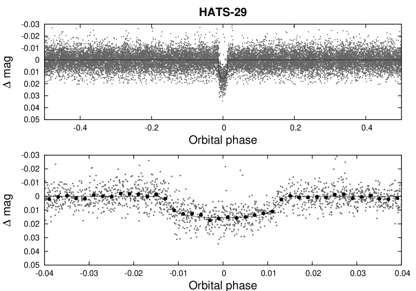
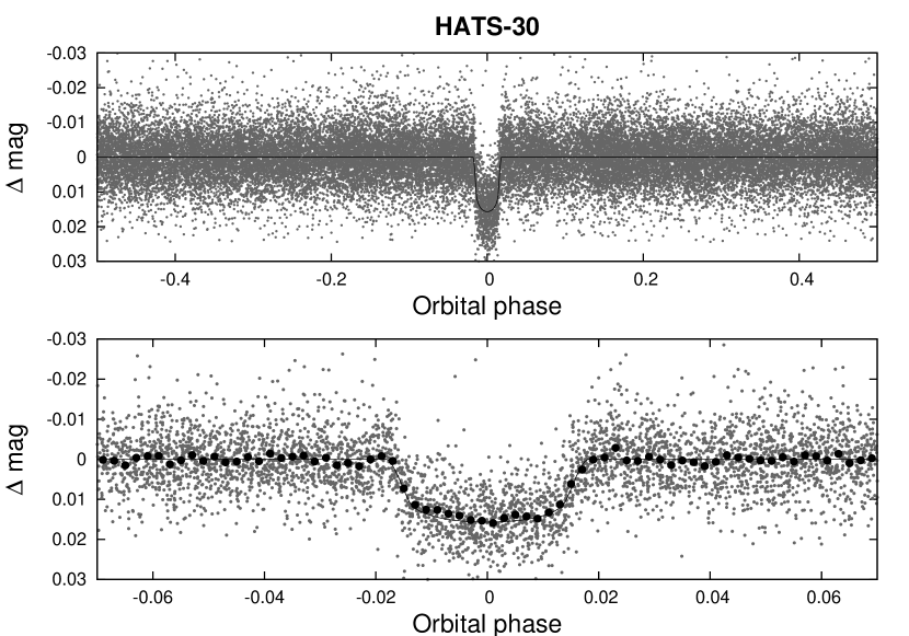
Figure 1.— Phase-folded unbinned HATSouth light curves for the six new transiting planet systems. In each case we show two panels. The top panel shows the full light curve, while the bottom panel shows the light curve zoomed-in on the transit. The solid lines show the model fits to the light curves. The dark filled circles in the bottom panels show the light curves binned in phase with a bin size of 0.002.

Table 1 Summary of photometric observations

Instrument/Field	Date(s)	# Images	Cadence	Filter	Precision
			(s)		(mmag)
HATS-25
HS-2.1/G568	2011 Mar–2011 Aug	5055	290	$r$	6.9
HS-4.1/G568	2011 Jul–2011 Aug	841	301	$r$	7.8
HS-6.1/G568	2011 May	131	289	$r$	9.3
LCOGT 1 m+CTIO/sinistro	2015 Feb 23	70	226	$i$	1.1
LCOGT 1 m+SSO/SBIG	2015 Mar 16	104	196	$i$	2.3
HATS-26
HS-2.3/G606	2012 Feb–2012 Jun	3134	291	$r$	7.0
HS-4.3/G606	2012 Feb–2012 Jun	2761	300	$r$	7.1
HS-6.3/G606	2012 Feb–2012 Jun	1170	299	$r$	6.8
LCOGT 1 m+SAAO/SBIG	2015 Mar 16	30	199	$i$	1.8
LCOGT 1 m+SAAO/SBIG	2015 Mar 26	46	137	$i$	2.0
LCOGT 1 m+CTIO/sinistro	2015 Apr 19	93	166	$i$	1.0
LCOGT 1 m+CTIO/sinistro	2015 May 21	40	165	$i$	1.7
LCOGT 1 m+SSO/SBIG	2015 Jun 04	110	73	$i$	2.9
HATS-27
HS-2.1/G700	2011 Apr–2012 Jul	4603	292	$r$	6.3
HS-4.1/G700	2011 Jul–2012 Jul	3851	301	$r$	7.5
HS-6.1/G700	2011 May–2012 Jul	1512	300	$r$	7.1
PEST 0.3 m	2015 Mar 12	141	132	$R_{C}$	4.1
LCOGT 1 m+SSO/SBIG	2015 Apr 09	282	75	$i$	2.3
HATS-28
HS-1.2/G747	2013 Mar–2013 Oct	4086	287	$r$	12.8
HS-2.2/G747	2013 Sep–2013 Oct	650	287	$r$	11.5
HS-3.2/G747	2013 Apr–2013 Nov	9051	297	$r$	12.1
HS-4.2/G747	2013 Sep–2013 Nov	1464	297	$r$	12.5
HS-5.2/G747	2013 Mar–2013 Nov	6018	297	$r$	10.7
HS-6.2/G747	2013 Sep–2013 Nov	1576	290	$r$	11.4
LCOGT 1 m+CTIO/sinistro	2015 Aug 31	38	223	$i$	1.4
LCOGT 1 m+CTIO/sinistro	2015 Sep 03	55	223	$i$	1.4
HATS-29
HS-1.1/G747	2013 Apr–2013 May	828	289	$r$	7.2
HS-2.1/G747	2013 Sep–2013 Oct	1331	287	$r$	7.5
HS-3.1/G747	2013 Apr–2013 Nov	9121	297	$r$	6.1
HS-4.1/G747	2013 Sep–2013 Nov	1505	297	$r$	8.2
HS-5.1/G747	2013 Mar–2013 Nov	6045	297	$r$	6.4
HS-6.1/G747	2013 Sep–2013 Nov	1544	290	$r$	7.2
LCOGT 1 m+CTIO/sinistro	2015 Jun 01	90	166	$i$	1.2
LCOGT 1 m+CTIO/sinistro	2015 Jun 24	36	162	$i$	1.0
HATS-30
HS-2.3/G754	2012 Sep–2012 Dec	3869	282	$r$	6.1
HS-6.3/G754	2012 Sep–2012 Dec	3000	285	$r$	6.2
HS-2.4/G754	2012 Sep–2012 Dec	3801	282	$r$	6.0
HS-4.4/G754	2012 Sep–2013 Jan	2820	292	$r$	6.6
HS-6.4/G754	2012 Sep–2012 Dec	2977	285	$r$	5.7
HS-1.1/G755	2011 Jul–2012 Oct	5180	291	$r$	9.2
HS-3.1/G755	2011 Jul–2012 Oct	4204	287	$r$	7.4
HS-5.1/G755	2011 Jul–2012 Oct	4904	296	$r$	6.5
LCOGT 1 m+SAAO/SBIG	2014 Oct 19	50	196	$i$	1.2
LCOGT 1 m+CTIO/sinistro	2014 Oct 23	56	226	$i$	1.0

2.2. Spectroscopic Observations

The spectroscopic observation of our planetary candidates is a two-step process. The first step is “reconnaissance” spectroscopy, which consists of observations used both to rule out false positive scenarios produced by certain configurations of stellar binaries that could mimic the detected transit features, and to estimate rough spectral parameters in order to estimate the physical and orbital parameters of the transiting planet candidates. The second step consists of spectroscopic observations that allow us to both confirm the planetary nature of the companion by radial velocity (RV) variations of the star due to the reflex motion produced by the planetary companion (which allows us to estimate its mass) and also to obtain precise stellar parameters from spectroscopic observables in order to derive absolute parameters of the planetary companion. The spectroscopic observations are summarized in Table 2, and are detailed below.

2.2.1 Reconnaissance spectroscopy

The reconnaissance spectroscopy of our candidates was made using the Wide Field Spectrograph (WiFeS, Dopita et al., 2007), located on the ANU $2.3$m telescope. Details of the observing strategy, reduction methods and the processing of the spectra for this instrument can be found in Bayliss et al. (2013). In summary, the observing strategy usually consists in taking data with two resolutions: $R=\lambda/\Delta\lambda=7000$ (medium) and $R=3000$ (low). The former are used to search for RV variations at the $\sim 2$ km/s level in order to rule out possible stellar companions, while the latter are used to estimate the spectroscopic parameters of the host stars. The results for each star were as follows:

• HATS-25: four medium resolution spectra and one low resolution spectrum were obtained. From these, a temperature of $5830\pm 300$ K, $\log(g)$ of $4.4\pm 0.3$, metallicity of $[\textnormal{Fe/H}]=0.0\pm 0.5$ was derived, implying that the star was a G-type star. No RV variations at the $\sim 2$ km/s level were found.

• HATS-26: two medium resolution spectra and one low resolution spectrum were obtained. No RV variation at the $\sim 2$ km/s level was found, and a temperature of $6333\pm 300$ K, $\log(g)$ of $4.1\pm 0.3$ and a metallicity of $[\textnormal{Fe/H}]=0.0\pm 0.5$ was derived, which pointed to an F-type star.

• HATS-27: three medium resolution and one low resolution spectra were obtained. We found no variation at the $\sim 2$ km/s level, and a temperature of $6683\pm 300$ K, $\log(g)$ of $4.5\pm 0.3$ and a metallicity of $[\textnormal{Fe/H}]=0.0\pm 0.5$ was derived for this star, implying it was consistent with being an F-type star.

• HATS-28: only one low resolution spectrum was obtained. With it, we derived a temperature of $5800\pm 300$ K, $\log(g)$ of $4.5\pm 0.3$ and a metallicity of $[\textnormal{Fe/H}]=0.0\pm 0.5$, hinting that this star was a G-type star.

• HATS-29: four medium resolution spectra and one low resolution spectrum were obtained. No variations at the $\sim 2$ km/s level were found, and we derived a temperature of $5658\pm 300$ K, $\log(g)$ of $4.5\pm 0.3$ and a metallicity of $[\textnormal{Fe/H}]=0.0\pm 0.5$, for this star, finding it to be a G-type star.

• HATS-30: three medium resolution spectra and one low resolution spectrum were obtained. No variations at the $\sim 2$ km/s level in the RVs were found. A temperature of $6155\pm 300$ K, $\log(g)$ of $4.6\pm 0.3$ and a metallicity of $[\textnormal{Fe/H}]=0.0\pm 0.5$ was derived, which suggested the star was either a hot G-type or a cool F-type star.

Given these results, our planet candidates were then promoted to our list requiring high-resolution spectroscopy and high precision photometric follow-up observations, which we now detail.

2.2.2 High-precision spectroscopy

High-precision spectroscopy was obtained for our targets with different instruments. Several $R=115000$ spectra were taken with the High Accuracy Radial Velocity Planet Searcher (HARPS, Mayor et al., 2003) on the ESO $3.6$m telescope at La Silla Observatory (LSO) between February 2015 and March 2016 in order to obtain high-precision RVs for HATS-25, HATS-26, HATS-27 and HATS-29. Spectra with $R=48000$ were also taken with the FEROS spectrograph (Kaufer & Pasquini, 1998) mounted on the MPG $2.2$m telescope at LSO between July 2014 and July 2015 in order to both extract precise spectroscopic parameters of the host stars (see Section 3) and obtain precise RVs for all of our targets. In addition, $R=60000$ spectra were also taken with the CORALIE (Queloz et al., 2001) spectrograph mounted on the 1.2m Euler telescope at LSO between June and November of 2014 for HATS-26, HATS-27, HATS-29 and HATS-30. The reduction of the CORALIE, FEROS and HARPS spectra followed the procedures described in Jordán et al. (2014) for CORALIE, and adapted to FEROS and HARPS. Finally, eight $R=70000$ spectra were obtained for HATS-29 on May 2015 to measure RVs, using the CYCLOPS2 fibre feed with the UCLES spectrograph on the $3.9$m Anglo-Australian Telescope (AAT); the data was reduced following the methods detailed in Addison et al. (2013).

The phased high-precision RV and bisector span (BS) measurements are shown for each system in Figure 2, while the data are listed in Table 8. It is important to note that the large observed scatter and errorbars on the RVs obtained from FEROS for HATS-27 are both due to the hot temperature of the star and due to contamination by scattered moonlight. Despite of this, it is evident that all the candidates show RV variations that are in phase with the photometric ephemeris. In addition, computed correlation coefficients between the RV and the BS measurements are all consistent with zero.

Table 2 Summary of spectroscopy observations

Instrument	UT Date(s)	# Spec.	Res.	S/N Range	$\gamma_{\rm RV}$	RV Precision
			$\Delta\lambda$/$\lambda$/1000		($\rm km\,s^{-1}$)	($\rm m\,s^{-1}$)
HATS-25
ANU 2.3 m/WiFeS	2014 Jun–Aug	4	7	26–152	30.0	4000
ANU 2.3 m/WiFeS	2014 Aug 5	1	3	88	$\cdots$	$\cdots$
ESO 3.6 m/HARPS	2015 Feb–Apr	8	115	11–23	31.663	8.8
MPG 2.2 m/FEROS	2015 Apr 9	1	48	64	31.649	20
HATS-26
ANU 2.3 m/WiFeS	2014 Jun 3–5	2	7	95–107	-14.4	4000
ANU 2.3 m/WiFeS	2014 Jun 4	1	3	121	$\cdots$	$\cdots$
Euler 1.2 m/Coralie	2014 Jun 19–21	2	60	17–19	-12.489	5.2
MPG 2.2 m/FEROS	2015 Jan–Feb	8	48	56–74	-12.516	21.0
ESO 3.6 m/HARPS	2015 Feb 14–19	4	115	19–23	-12.561	21.3
HATS-27
ANU 2.3 m/WiFeS	2014 Jun 2	1	3	50	$\cdots$	$\cdots$
ANU 2.3 m/WiFeS	2014 Jun 3–5	3	7	4.6–12	-7.6	4000
Euler 1.2 m/Coralie	2014 Jun 20–21	3	60	21–22	-3.521	66
MPG 2.2 m/FEROS	2014 Jul–2015 Apr	15	48	18–92	-3.525	78
ESO 3.6 m/HARPS	2014 Aug–2016 Mar	11	115	4–25	-3.582	35
HATS-28
ANU 2.3 m/WiFeS	2015 Jun 1	1	3	38	$\cdots$	$\cdots$
MPG 2.2 m/FEROS	2015 Jun–Jul Apr	18	48	17–52	-8.651	38
HATS-29
ANU 2.3 m/WiFeS	2014 Dec–2015 Mar	4	7	3.1–31	-17.5	4000
ANU 2.3 m/WiFeS	2015 Mar 2	1	3	45	$\cdots$	$\cdots$
ESO 3.6 m/HARPS	2015 Apr 6–8	3	115	12–23	-19.719	18
AAT 3.9 m/CYCLOPS	2015 May 6–9	9	70	16–30	-19.722	40
Euler 1.2 m/Coralie	2014 Jun 20–21	4	60	16–19	-19.698	11
MPG 2.2 m/FEROS	2015 Jun 13	3	48	48–50	-19.670	20
HATS-30
MPG 2.2 m/FEROS	2014 Oct–Dec	7	48	60–96	-0.079	8.3
ANU 2.3 m/WiFeS	2014 Oct 4	1	3	233	$\cdots$	$\cdots$
ANU 2.3 m/WiFeS	2014 Oct 4–10	3	7	87–118	1.4	4000
Euler 1.2 m/Coralie	2014 Oct–Nov	6	60	22–30	-0.112	22

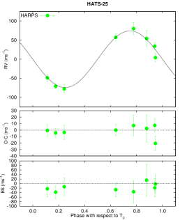
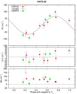
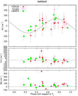
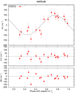
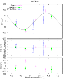
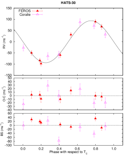
Figure 2.— Phased high-precision RV measurements for the six new transiting planet systems. The instruments used are labelled in the plots. In each case we show three panels. The top panel shows the phased measurements together with our best-fit circular-orbit model (see Table 6) for each system. Zero-phase corresponds to the time of mid-transit. The center-of-mass velocity has been subtracted. The second panel shows the velocity $O\!-\!C$ residuals from the best fit. The error bars include the jitter terms listed in Tables 6 and 7 added in quadrature to the formal errors for each instrument. The third panel shows the bisector spans (BS). Note the different vertical scales of the panels.

2.3. Photometric follow-up observations

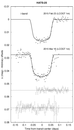
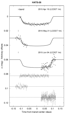
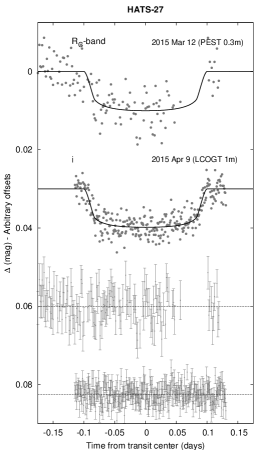
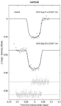
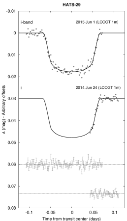
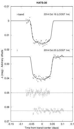
Figure 3.— Unbinned transit light curves for the six new transiting planet systems. The light curves have been corrected for quadratic trends in time fitted simultaneously with the transit model, and for correlations with up to three parameters describing the shape of the PSF. The dates of the events, filters and instruments used are indicated. Light curves following the first are displaced vertically for clarity. Our best fit from the global modeling described in Section 3.3 is shown by the solid lines. The residuals from the best-fit model are shown below in the same order as the original light curves. The error bars represent the photon and background shot noise, plus the readout noise. Note the differing vertical and horizontal scales used for each system. For HATS-25 we do not show the LCOGT 1 m light curves from UT 2015 Mar 16 and 26 which were taken entirely out of transit.

Photometric follow-up for the six systems was obtained in order to (1) rule out possible false positive scenarios not identified in our reconnaissance spectroscopy (e.g., blended eclipsing binaries, hierarchical triples) that would leave signatures in the transit events (e.g., significantly different depths between different bands), (2) refine the ephemerides and (3) refine the derived transit parameters obtained from the HATSouth discovery lightcurves. Our photometric follow-up observations are summarized in Table 1 and plotted in Figure 3.

Photometry for these six systems was obtained mainly from 1m-class telescopes at different sites of the Las Cumbres Observatory Global Telescope (LCOGT) network (Brown et al., 2013), using the $i$ filter (each of the sites used are indicated in Table 1). In particular, one partial transit and a full transit was observed for HATS-25b on February 2015 and March 2015 respectively, three partial transits were observed for HATS-26b on April, May and June of 2015, one full transit was observed for HATS-27b on April 2015, two partial transits were observed for HATS-28b on August and September of 2015, one full transit and a partial transit was observed for HATS-29b on June 2015 and 2014, respectively, and two partial transits were observed for HATS-30b on October 2014. In addition, one full transit of HATS-27b was observed using the $0.3m$ Perth Exoplanet Survey Telescope (PEST) on March of 2015. The instrument specifications, observing strategies and reduction of the data have been previously described in Bayliss et al. (2015) for the LCOGT data and in Zhou et al. (2014) for the PEST data.

2.4. Lucky imaging observations

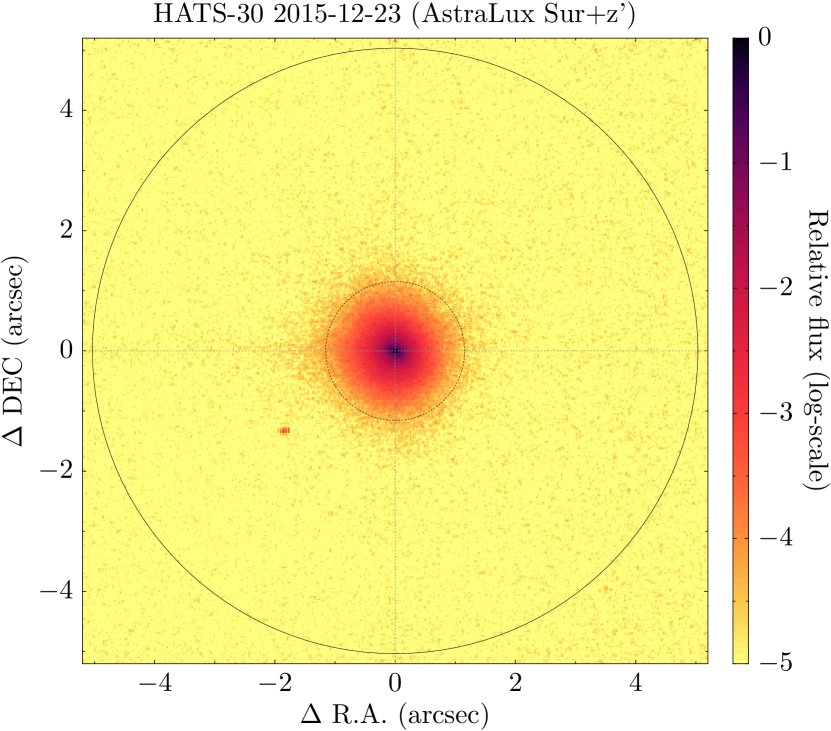
Figure 4.— (Left) AstraLux Sur $z^{\prime}$-band observations of HATS-26. Circles of $1^{\prime\prime}$ radius (approximately the mean FWHM measured for the image) and $5^{\prime\prime}$ radius are shown for reference on the images. The central lines indicate the fitted center of the star with our PSF modelling (see text). (Right) Same image but for HATS-30. Note the difference in the shape of the PSF, which is a purely instrumental effect.

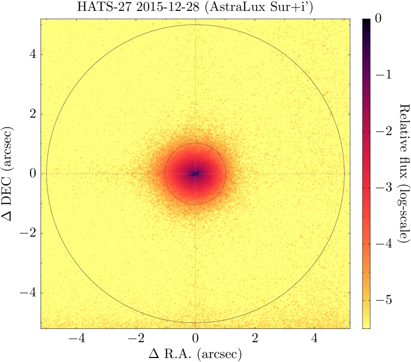
Figure 5.— AstraLux Sur $i^{\prime}$-band observations of HATS-27. The circles and lines indicate the same distances and positions as the ones described in Figure 4.

As part of a systematic program of obtaining high spatial resolution imaging for HATSouth candidates, “lucky” imaging observations were obtained for HATS-26, HATS-27 and HATS-30 using the Astralux Sur camera (Hippler et al., 2009) mounted on the New Technology Telescope (NTT) at La Silla Observatory, in Chile on December 23 and 28, 2015.

Both the HATS-26 and HATS-30 datasets, obtained on December 23, were obtained using the SDSS $z^{\prime}$ filter, while the HATS-27 dataset, obtained on December 28, was obtained using the SDSS $i^{\prime}$ filter. A drizzle algorithm (Fruchter & Hook, 2002) was used to combine the images, selecting the best of them from the set of $\sim 10^{4}$ exposures taken for each target ($10^{4}$ images with an exposure time of 40 ms each for HATS-26, $2\times 10^{4}$ images with an exposure time of 15 ms each for HATS-27 and $2\times 10^{4}$ images with an exposure time of 15 ms each for HATS-30). Figure 4 shows the resulting images for HATS-26 and HATS-30 and Figure 5 shows the resulting image for HATS-27, all of which are the combination of the best $10\%$ of the images acquired for each target. The resulting images show an asymmetric extended profile for HATS-26 (a purely instrumental effect as confirmed by taking images of other targets on different nights), whereas the profile is fairly symmetric for HATS-27 and HATS-30 (we note that the latter shows an instrumental artefact close to $(-2,-2)$ arcsecs from the target star). As can be seen from our images, no obvious companions were detected out to a $5\arcsec$ radius.

In order to extract quantitative information from these images, we generated $5\sigma$ contrast curves for each of our targets, which required us to model the Point Spread Functions (PSFs). We decided to model the PSFs of our targets as a weighted sum of a Moffat profile (which models the central part of the PSF) and an asymmetric Gaussian (to model asymmetries in the PSF wings). The full width at half maximum (FWHM) of the full model was measured numerically at 100 different angles by finding the points at which the model has half of the peak flux, and the median of these measurements (the “effective” FWHM, $\rm{FWHM}_{\rm eff}$) is taken as the resolution limit of our observations. For HATS-26, we found $\rm{FWHM}_{\rm eff}=3.27\pm 0.35$ pixels, which given the pixel scale of $23$ milli-arcseconds (mas) per pixel, gives a resolution limit of $75\pm 8$ mas. For HATS-27, we found $\rm{FWHM}_{\rm eff}=3.17\pm 0.28$ pixels, which implies a resolution limit of $72\pm 6$ mas. Finally, for HATS-30, $\rm{FWHM}_{\rm eff}=3.55\pm 0.29$ pixels, which implies a resolution limit of $81\pm 7$ mas. All the effective FWHMs are close to the diffraction limit of the instrument, which is $\sim 50$ mas (Hippler et al., 2009).

Once modelled, we subtracted the PSF of the target stars from the images and generated the contrast curves by an “injection and recovery” approach, in which we injected signals with the same fitted PSF parameters at different positions ($r$,$\theta$) in the image, where $r$ is the distance from the target star and $\theta$ is the azimuthal angle around it. We sampled $r$ in steps of $\rm{FWHM}_{\rm eff}$, while the angles are sampled at each radius covering $2\pi$ radians with independent regions of arc-length equal to $\rm{FWHM}_{\rm eff}$. The injected sources were scaled in order to simulate a wide range of contrasts, exploring from $\Delta z^{\prime}=0$ to $\Delta z^{\prime}=10$ in $0.01$ steps, where $\Delta z^{\prime}$ is the magnitude contrast with respect to the target star. We considered an injected source to be detectable if five or more pixels were $5\sigma$ above the noise level, which was estimated as the standard deviation in a box of size $\rm{FWHM}_{\rm eff}\times\rm{FWHM}_{\rm eff}$ at each position in the residual image at which the signals were injected. Finally, the contrast at each radius was obtained by averaging the azimuthal contrasts and the standard deviation of these azimuthal contrasts was taken as the error on the contrast at each radius. The resulting contrast curves for HATS-26 (blue) and HATS-30 (orange) are shown on Figure 6, where the grey bands show the uncertainty of the contrast at each radius. The corresponding contrast curve for HATS-27 is shown in Figure 7. Code to model the PSFs of images as explained here and to generate these contrast curves can be found at https://github.com/nespinoza/luckyimg-reduction.

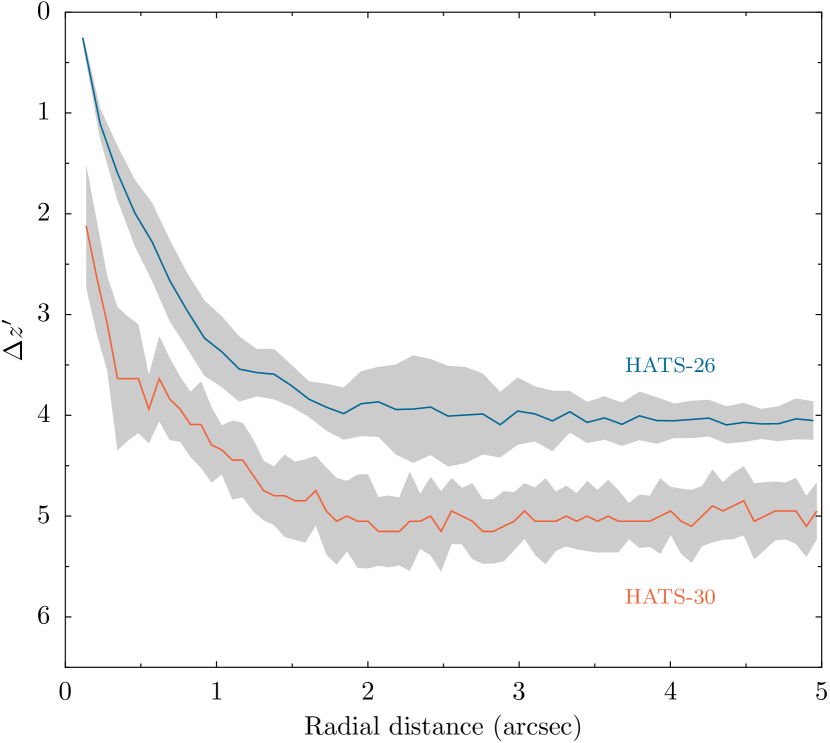
Figure 6.— Contrast curves generated for HATS-26 (blue) and HATS-30 (orange) using our AstraLux Sur $z^{\prime}$-band observations. Gray bands show the uncertainty given by the scatter in the contrast in the azimuthal direction at a given radius (see text for details).

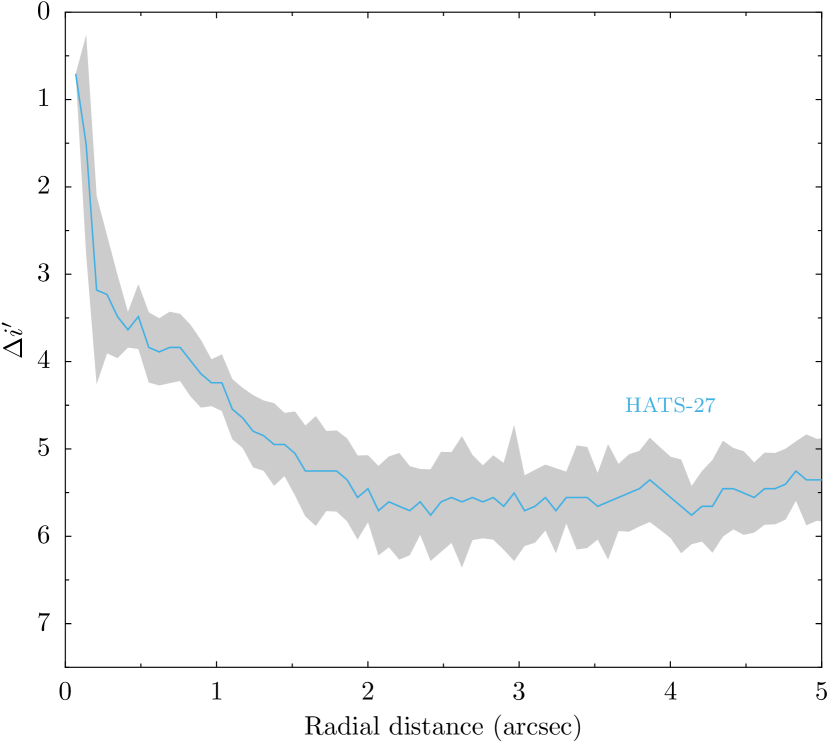
Figure 7.— Contrast curve generated for HATS-27 using our AstraLux Sur $i^{\prime}$-band observations. Gray bands show the uncertainty given by the scatter in the contrast in the azimuthal direction at a given radius (see text for details).

Table 3 Light curve data for HATS-25–HATS-30.

Object	BJD	Mag	$\sigma_{\rm Mag}$	Mag(orig)	Filter	Instrument
	(2,400,000$+$)
HATS-27	$56076.42690$	$0.00302$	$0.00469$	$\cdots$	$r$	HS
HATS-27	$56090.33807$	$0.00531$	$0.00449$	$\cdots$	$r$	HS
HATS-27	$55955.86458$	$-0.00442$	$0.00406$	$\cdots$	$r$	HS
HATS-27	$56113.52396$	$0.00956$	$0.00462$	$\cdots$	$r$	HS
HATS-27	$56016.14672$	$0.00478$	$0.00406$	$\cdots$	$r$	HS
HATS-27	$56062.51729$	$-0.00009$	$0.00864$	$\cdots$	$r$	HS
HATS-27	$56020.78399$	$0.00065$	$0.00445$	$\cdots$	$r$	HS
HATS-27	$56006.87363$	$-0.01152$	$0.00436$	$\cdots$	$r$	HS
HATS-27	$56030.05986$	$-0.00319$	$0.00425$	$\cdots$	$r$	HS
HATS-27	$56076.43037$	$0.00830$	$0.00472$	$\cdots$	$r$	HS

Note. — This table is available in a machine-readable form in the online journal. A portion is shown here for guidance regarding its form and content.

3. Analysis

3.1. Properties of the parent stars

We determine the properties of the host stars using the Zonal Atmospherical Stellar Parameter Estimator (ZASPE, Brahm et al., in preparation) on median combined FEROS spectra for all our systems except for HATS-25, where only one FEROS spectrum was used. With the effective temperature ($T_{\textnormal{eff}*}$), log-gravity ($\log{g_{\star}}$) metallicity ([Fe/H]) and the projected stellar rotational velocity of the star ($v\sin i$) calculated for each of our systems, the Yonsei-Yale (Y², Yi et al., 2001) isochrones were used to obtain the physical parameters of the host stars. However, instead of using $\log{g_{\star}}$ to search for the best-fit isochrone, we follow Sozzetti et al. (2007) in using the stellar density ($\rho_{*}$), which is well constrained parameter by our transit fits. Once this was done and physical parameters were found, a second ZASPE iteration was done for all systems except for HATS-27, for which a second iteration did not improve the results. In this second iteration, the revised value of $\log{g_{\star}}$ was used as input in order to derive the final properties of the stars. In order to calculate the distances to these stars, we compared their measured broad-band photometry to the predicted magnitudes in each filter from the isochrones, assuming an extinction law from Cardelli et al. (1989) with $R_{V}=3.1$. The resulting parameters for HATS-25, HATS-26 and HATS-27 are given in Table 4, and for HATS-28, HATS-29 and HATS-30 in Table 5. The locations of each star on an $T_{\rm eff\star}$–$\rho_{\star}$ diagram (similar to a Hertzsprung-Russell diagram) are shown in Figure 8.

It is interesting to note that while HATS-25, HATS-28, HATS-29 and HATS-30 are typical G dwarfs, HATS-26 and HATS-27 stand out as slightly evolved F stars which are just after and in the turn-off points, respectively. Consequently, they have radii of $2.04^{+0.15}_{-0.11}R_{\sun}$ and $1.74^{+0.17}_{-0.10}R_{\sun}$ which (combined with their effective temperatures of $6071\pm 81$ K and $6438\pm 64$ K, respectively) implies relatively large luminosities of $5.06^{+0.90}_{-0.64}L_{\sun}$ and $4.67^{+0.92}_{-0.58}L_{\sun}$. Because of this, their planets receive larger insolation levels than typical hot Jupiters with the same periods.

Figure 8.— Model isochrones from Yi et al. (2001) for the measured metallicities of each of the six new transiting planet host stars. We show models for ages of 0.2 Gyr and 1.0 to 14.0 Gyr in 1.0 Gyr increments (ages increasing from left to right). The adopted values of $T_{\rm eff\star}$ and $\rho_{\star}$ are shown together with their 1$\sigma$ and 2$\sigma$ confidence ellipsoids. The initial values of $T_{\rm eff\star}$ and $\rho_{\star}$ from the first ZASPE and light curve analyses are represented with a triangle.

Table 4 Stellar parameters for HATS-25, HATS-26 and HATS-27

	HATS-25	HATS-26	HATS-27
Parameter	Value	Value	Value	Source
Astrometric properties and cross-identifications
2MASS-ID	2MASS 13513786-2346522	2MASS 09394244-2835081	2MASS 12541261-4635157
GSC-ID	GSC 6716-01190	GSC 6614-01083	GSC 8245-02236
R.A. (J2000)	$13^{\mathrm{h}}51^{\mathrm{m}}37.80{\mathrm{s}}$	$09^{\mathrm{h}}39^{\mathrm{m}}42.44{\mathrm{s}}$	$12^{\mathrm{h}}54^{\mathrm{m}}12.60{\mathrm{s}}$	2MASS
Dec. (J2000)	$-23{\arcdeg}46{\arcmin}52.2{\arcsec}$	$-28{\arcdeg}35{\arcmin}08.1{\arcsec}$	$-46{\arcdeg}35{\arcmin}15.8{\arcsec}$	2MASS
$\mu_{\rm R.A.}$ ($\rm mas\,yr^{-1}$)	$-20.5\pm 1.0$	$-1.3\pm 1.4$	$-10.2\pm 1.1$	UCAC4
$\mu_{\rm Dec.}$ ($\rm mas\,yr^{-1}$)	$-11.9\pm 1.1$	$-6.1\pm 1.3$	$4.7\pm 1.1$	UCAC4
Spectroscopic properties
$T_{\rm eff\star}$ (K)	$5715\pm 73$	$6071\pm 81$	$6438\pm 64$	ZASPE
$\rm[Fe/H]$	$0.020\pm 0.050$	$-0.020\pm 0.050$	$0.090\pm 0.040$	ZASPE
$v\sin{i}$ ($\rm km\,s^{-1}$)	$3.88\pm 0.50$	$7.48\pm 0.50$	$9.32\pm 0.50$	ZASPE
$v_{\rm mac}$ ($\rm km\,s^{-1}$)	$3.90$	$4.44$	$5.01$	Assumed
$v_{\rm mic}$ ($\rm km\,s^{-1}$)	$1.04$	$1.29$	$1.67$	Assumed
$\gamma_{\rm RV}$ ($\rm m\,s^{-1}$)	$31663.2\pm 3.6$	$-12515.9\pm 6.7$	$-3582\pm 12$	FEROS or HARPS
Photometric properties
$B$ (mag)	$13.812\pm 0.030$	$13.553\pm 0.030$	$13.239\pm 0.050$	APASS
$V$ (mag)	$13.097\pm 0.030$	$12.955\pm 0.030$	$12.766\pm 0.040$	APASS
$g$ (mag)	$13.380\pm 0.020$	$13.229\pm 0.010$	$12.927\pm 0.040$	APASS
$r$ (mag)	$12.909\pm 0.040$	$12.822\pm 0.010$	$12.665\pm 0.040$	APASS
$i$ (mag)	$12.687\pm 0.050$	$12.695\pm 0.030$	$12.515\pm 0.080$	APASS
$J$ (mag)	$11.788\pm 0.022$	$11.839\pm 0.024$	$11.831\pm 0.022$	2MASS
$H$ (mag)	$11.487\pm 0.024$	$11.510\pm 0.024$	$11.651\pm 0.023$	2MASS
$K_{s}$ (mag)	$11.416\pm 0.021$	$11.435\pm 0.021$	$11.550\pm 0.023$	2MASS
Derived properties
$M_{\star}$ ($M_{\sun}$)	$0.994\pm 0.035$	$1.299_{-0.056}^{+0.113}$	$1.415\pm 0.048$	YY+$\rho_{\star}$+ZASPE
$R_{\star}$ ($R_{\sun}$)	$1.107\pm 0.069$	$2.04_{-0.11}^{+0.15}$	$1.74_{-0.10}^{+0.17}$	YY+$\rho_{\star}$+ZASPE
$\log{g_{\star}}$ (cgs)	$4.347\pm 0.053$	$3.936\pm 0.046$	$4.107\pm 0.049$	YY+$\rho_{\star}$+ZASPE
$\rho_{\star}$ ($\rm g\,cm^{-3}$)	$1.03\pm 0.20$	$0.219\pm 0.033$	$0.380\pm 0.063$	Light curves
$\rho_{\star}$ ($\rm g\,cm^{-3}$)	$1.03\pm 0.20$	$0.218\pm 0.034$	$0.379\pm 0.064$	YY+Light curves+ZASPE
$L_{\star}$ ($L_{\sun}$)	$1.17\pm 0.17$	$5.06_{-0.64}^{+0.90}$	$4.67_{-0.58}^{+0.92}$	YY+$\rho_{\star}$+ZASPE
$M_{V}$ (mag)	$4.67\pm 0.16$	$3.03\pm 0.17$	$3.06\pm 0.17$	YY+$\rho_{\star}$+ZASPE
$M_{K}$ (mag,ESO)	$3.10\pm 0.14$	$1.68\pm 0.15$	$1.98\pm 0.15$	YY+$\rho_{\star}$+ZASPE
Age (Gyr)	$7.5\pm 1.9$	$4.04_{-0.94}^{+0.62}$	$2.30\pm 0.22$	YY+$\rho_{\star}$+ZASPE
$A_{V}$ (mag)	$0.083\pm 0.061$	$0.140\pm 0.070$	$0.084\pm 0.066$	YY+$\rho_{\star}$+ZASPE
Distance (pc)	$466\pm 30$0	$907_{-49}^{+69}$	$840_{-51}^{+80}$	YY+$\rho_{\star}$+ZASPE

Note. — For HATS-25 and HATS-26 the fixed-circular-orbit model has a higher Bayesian evidence than the eccentric-orbit model (it is 10 and 8 times greater for these two systems respectively). We therefore assume a fixed circular orbit in generating the parameters listed for both of these systems. For HATS-27 the free-eccentricity model has an indistinguishable Bayesian evidence from the fixed-circular model, but in this case the eccentricity is poorly constrained with implausibly high values permitted by the low S/N RV measurements. For this system we also adopt the fixed-circular model parameters.

Table 5 Stellar parameters for HATS-28, HATS-29 and HATS-30

	HATS-28	HATS-29	HATS-30
Parameter	Value	Value	Value	Source
Astrometric properties and cross-identifications
2MASS-ID	2MASS 18573592-4908184	2MASS 19002314-5453354	2MASS 00222848-5956331
GSC-ID	GSC 8382-00661	GSC 8763-00475	GSC 8471-00231
R.A. (J2000)	$18^{\mathrm{h}}57^{\mathrm{m}}36.00{\mathrm{s}}$	$19^{\mathrm{h}}00^{\mathrm{m}}23.04{\mathrm{s}}$	$00^{\mathrm{h}}22^{\mathrm{m}}28.49{\mathrm{s}}$	2MASS
Dec. (J2000)	$-49{\arcdeg}08{\arcmin}18.5{\arcsec}$	$-54{\arcdeg}53{\arcmin}35.5{\arcsec}$	$-59{\arcdeg}56{\arcmin}33.2{\arcsec}$	2MASS
$\mu_{\rm R.A.}$ ($\rm mas\,yr^{-1}$)	$10.3\pm 1.6$	$2.8\pm 1.3$	$-25.3\pm 1.0$	UCAC4
$\mu_{\rm Dec.}$ ($\rm mas\,yr^{-1}$)	$-2.4\pm 1.4$	$-37.1\pm 3.7$	$-8.2\pm 1.0$	UCAC4
Spectroscopic properties
$T_{\rm eff\star}$ (K)	$5498\pm 84$	$5670\pm 110$	$5943\pm 70$	ZASPE
$\rm[Fe/H]$	$0.010\pm 0.060$	$0.160\pm 0.080$	$0.060\pm 0.050$	ZASPE
$v\sin{i}$ ($\rm km\,s^{-1}$)	$2.6\pm 1.0$	$2.35\pm 0.80$	$4.11\pm 0.50$	ZASPE
$v_{\rm mac}$ ($\rm km\,s^{-1}$)	$3.56$	$3.83$	$4.25$	Assumed
$v_{\rm mic}$ ($\rm km\,s^{-1}$)	$0.93$	$1.02$	$1.19$	Assumed
$\gamma_{\rm RV}$ ($\rm m\,s^{-1}$)	$-8650.5\pm 9.1$	$-19719.3\pm 6.9$	$-78.6\pm 4.2$	FEROS or HARPS
Photometric properties
$B$ (mag)	$14.697\pm 0.020$	$13.361\pm 0.010$	$12.790\pm 0.010$	APASS
$V$ (mag)	$13.934\pm 0.080$	$12.612\pm 0.010$	$12.192\pm 0.010$	APASS
$g$ (mag)	$14.274\pm 0.030$	$12.950\pm 0.010$	$12.439\pm 0.010$	APASS
$r$ (mag)	$13.717\pm 0.010$	$12.430\pm 0.010$	$12.046\pm 0.010$	APASS
$i$ (mag)	$13.615\pm 0.010$	$12.154\pm 0.010$	$11.935\pm 0.010$	APASS
$J$ (mag)	$12.522\pm 0.026$	$11.286\pm 0.026$	$11.129\pm 0.024$	2MASS
$H$ (mag)	$12.188\pm 0.025$	$10.933\pm 0.021$	$10.826\pm 0.024$	2MASS
$K_{s}$ (mag)	$12.086\pm 0.029$	$10.877\pm 0.019$	$10.793\pm 0.019$	2MASS
Derived properties
$M_{\star}$ ($M_{\sun}$)	$0.929\pm 0.036$	$1.032\pm 0.049$	$1.093\pm 0.031$	YY+$\rho_{\star}$+ZASPE
$R_{\star}$ ($R_{\sun}$)	$0.922\pm 0.040$	$1.073\pm 0.038$	$1.061\pm 0.039$	YY+$\rho_{\star}$+ZASPE
$\log{g_{\star}}$ (cgs)	$4.476\pm 0.039$	$4.389\pm 0.027$	$4.425\pm 0.030$	YY+$\rho_{\star}$+ZASPE
$\rho_{\star}$ ($\rm g\,cm^{-3}$)	$1.68\pm 0.27$	$1.17\pm 0.11$	$1.34\pm 0.19$	Light curves
$\rho_{\star}$ ($\rm g\,cm^{-3}$)	$1.67\pm 0.22$	$1.17\pm 0.11$	$1.29\pm 0.14$	YY+Light Curves+ZASPE
$L_{\star}$ ($L_{\sun}$)	$0.696\pm 0.084$	$1.07\pm 0.13$	$1.25\pm 0.12$	YY+$\rho_{\star}$+ZASPE
$M_{V}$ (mag)	$5.28\pm 0.14$	$4.77\pm 0.15$	$4.57\pm 0.12$	YY+$\rho_{\star}$+ZASPE
$M_{K}$ (mag,ESO)	$3.53\pm 0.10$	$3.166\pm 0.088$	$3.123\pm 0.088$	YY+$\rho_{\star}$+ZASPE
Age (Gyr)	$6.2\pm 2.8$	$5.5_{-1.7}^{+2.6}$	$2.3\pm 1.2$	YY+$\rho_{\star}$+ZASPE
$A_{V}$ (mag)	$0.055_{-0.055}^{+0.124}$	$0.111\pm 0.082$	$0.0000\pm 0.0066$	YY+$\rho_{\star}$+ZASPE
Distance (pc)	$521\pm 25$0	$351\pm 15$	$339\pm 16$	YY+$\rho_{\star}$+ZASPE

Note. — For all three systems the fixed-circular-orbit model has a higher Bayesian evidence than the eccentric-orbit model (it is 5, 660, and 3 times greater for HATS-28, HATS-29 and HATS-30, respectively). We therefore assume a fixed circular orbit in generating the parameters listed for these systems.

3.2. Excluding blend scenarios

In order to exclude blend scenarios we carried out an analysis following Hartman et al. (2012). We attempt to model the available photometric data (including light curves and catalog broad-band photometric measurements) for each object as a blend between an eclipsing binary star system and a third star along the line of sight. The physical properties of the stars are constrained using the Padova isochrones (Girardi et al., 2000), while we also require that the brightest of the three stars in the blend have atmospheric parameters consistent with those measured with ZASPE. We also simulate composite cross-correlation functions (CCFs) and use them to predict RVs and BSs for each blend scenario considered.

Based on this analysis we rule out blended stellar eclipsing binary scenarios for all six systems. However, in general we cannot rule out the possibility that one or more of these objects may be an unresolved binary star system with one component hosting a transiting planet, although limits can be placed on those scenarios for HATS-26, HATS-27 and HATS-30 based on our lucky imaging observations shown on Section 2.4. The results for each object are as follows:

• HATS-25: All blend models tested give higher $\chi^{2}$ than a model of single star with a planet. Those blend models which cannot be rejected with greater than $5\sigma$ confidence predict either RV or BS variations greater than 1 $\rm km\,s^{-1}$, which are excluded by the observations.

• HATS-26: All blend models tested can be rejected with greater than $5\sigma$ confidence based on the photometry alone. In particular, the blend models predict a large out-of-transit variation due to the tidal distortion of the binary star components. Such a variation is ruled out by the HATSouth photometry.

• HATS-27: Same conclusion as for HATS-25.

• HATS-28: All blend models tested can be rejected with greater than $4\sigma$ confidence based on the photometry alone.

• HATS-29: Blend models which cannot be rejected with greater than $5\sigma$ confidence based on the photometry alone generally predict large RV and BS variations exceeding 1 $\rm km\,s^{-1}$. There is a narrow region of parameter space where the blend models are rejected at $4\sigma$ confidence based on the photometry, and the simulated RVs and BSs have scatters of a few 100 $\rm m\,s^{-1}$, which is not much greater than the measured values. However, the simulated RVs do not phase with the photometric ephemeris.

• HATS-30: All blend models tested can be rejected with greater than $4\sigma$ confidence based on the photometry alone.

3.3. Global modeling of the data

We modeled the HATSouth photometry, the follow-up photometry, and the high-precision RV measurements following Pál et al. (2008); Bakos et al. (2010); Hartman et al. (2012). We fit Mandel & Agol (2002) transit models to the light curves, allowing for a dilution of the HATSouth transit depth as a result of blending from neighboring stars and over-correction by the trend-filtering method. For the follow-up light curves we include a quadratic trend in time, and linear trends with up to three parameters describing the shape of the PSF, in our model for each event to correct for systematic errors in the photometry. We fit Keplerian orbits to the RV curves allowing the zero-point for each instrument to vary independently in the fit, and allowing for RV jitter which we we also vary as a free parameter for each instrument. We used a Differential Evolution Markov Chain Monte Carlo procedure to explore the fitness landscape and to determine the posterior distributions of the parameters. Note that we tried fitting both fixed-circular-orbits and free-eccentricity models to the data, and for all six systems find that the data are consistent with a circular orbit. We estimate the Bayesian evidence for the fixed-circular and free-eccentricity models for each system, and find that in all six cases the fixed-circular model has greater evidence. In particular, for the HATS-25, HATS-26, HATS-28, HATS-29 and HATS-30 systems, the Bayesian evidence for the fixed-circular-orbit model is 10, 8, 5, 660 and 3 times greater, respectively, than the eccentric-orbit model, favouring the former in these cases. For HATS-27, both models are indistinguishable, but the eccentricity is poorly constrained by the data at hand, giving implausibly high values for it. We therefore adopt the parameters that come from the fixed-circular-orbit models for all of the systems. The resulting parameters for HATS-25b, HATS-26b and HATS-27b are listed in Table 6, while for HATS-28b, HATS-29b and HATS-30b they are listed in Table 7.

As can be observed from the tables, all the presented planets can be classified as typical hot Jupiters, with short-periods, similar masses of $\sim 0.6M_{J}$ and larger-than-Jupiter radii.

Table 6Orbital and planetary parameters for HATS-25b, HATS-26b and HATS-27b

	HATS-25b	HATS-26b	HATS-27b
Parameter	Value	Value	Value
Light curve parameters
$P$ (days)	$4.2986432\pm 0.0000045$	$3.3023881\pm 0.0000076$	$4.637038\pm 0.000014$
$T_{c}$ (${\rm BJD}$)	$2456870.36872\pm 0.00051$	$2456867.4232\pm 0.0012$	$2457029.3374\pm 0.0011$
$T_{14}$ (days)	$0.1335\pm 0.0025$	$0.2173\pm 0.0041$	$0.2013\pm 0.0033$
$T_{12}=T_{34}$ (days)	$0.0190\pm 0.0027$	$0.0196\pm 0.0035$	$0.0186\pm 0.0030$
$a/R_{\star}$	$10.03\pm 0.62$	$5.01\pm 0.27$	$7.55_{-0.59}^{+0.42}$
$\zeta/R_{\star}$	$17.39\pm 0.17$0	$10.14\pm 0.13$0	$10.98_{-0.14}^{+0.11}$0
$R_{p}/R_{\star}$	$0.1171\pm 0.0026$	$0.0879\pm 0.0055$	$0.0895\pm 0.0043$
$b^{2}$	$0.290_{-0.102}^{+0.087}$	$0.109_{-0.084}^{+0.098}$	$0.13_{-0.10}^{+0.13}$
$b\equiv a\cos i/R_{\star}$	$0.538_{-0.105}^{+0.075}$	$0.33_{-0.17}^{+0.12}$	$0.36_{-0.19}^{+0.15}$
$i$ (deg)	$86.93\pm 0.71$0	$86.2\pm 1.9$0	$87.3\pm 1.3$0
HATSouth blend factors
Blend factor	$0.959\pm 0.046$	$0.775\pm 0.077$	$0.778\pm 0.086$
Limb-darkening coefficients
$c_{1},R$	$\cdots$	$\cdots$	$0.2295$
$c_{2},R$	$\cdots$	$\cdots$	$0.3855$
$c_{1},r$	$0.3674$	$0.2947$	$0.2511$
$c_{2},r$	$0.3192$	$0.3611$	$0.3857$
$c_{1},i$	$0.2774$	$0.2145$	$0.1754$
$c_{2},i$	$0.3246$	$0.3580$	$0.3788$
RV parameters
$K$ ($\rm m\,s^{-1}$)	$76.8\pm 5.0$00	$73.3\pm 8.0$00	$51\pm 13$00
$e$	$<0.176$	$<0.245$	$<0.581$
RV jitter FEROS ($\rm m\,s^{-1}$)	$\cdots$	$<28$	$72\pm 17$
RV jitter HARPS ($\rm m\,s^{-1}$)	$<0.12$	$<9.1$	$<38.0$
RV jitter Coralie ($\rm m\,s^{-1}$)	$\cdots$	$<8.1$	$<142.2$
Planetary parameters
$M_{p}$ ($M_{\rm J}$)	$0.613\pm 0.042$	$0.650\pm 0.076$	$0.53\pm 0.13$
$R_{p}$ ($R_{\rm J}$)	$1.26\pm 0.10$	$1.75\pm 0.21$	$1.50_{-0.11}^{+0.20}$
$C(M_{p},R_{p})$	$0.01$	$0.27$	$-0.00$
$\rho_{p}$ ($\rm g\,cm^{-3}$)	$0.38\pm 0.10$	$0.153\pm 0.042$	$0.180_{-0.057}^{+0.083}$
$\log g_{p}$ (cgs)	$2.976\pm 0.075$	$2.724_{-0.103}^{+0.074}$	$2.75\pm 0.15$
$a$ (AU)	$0.05163\pm 0.00060$	$0.04735_{-0.00068}^{+0.00133}$	$0.06110\pm 0.00068$
$T_{\rm eq}$ (K)	$1277\pm 42$	$1918\pm 61$	$1659_{-46}^{+66}$
$\Theta$	$0.0500\pm 0.0054$	$0.0264\pm 0.0038$	$0.0292\pm 0.0081$
$\log_{10}\langle F\rangle$ (cgs)	$8.778\pm 0.057$	$9.485\pm 0.054$	$9.232_{-0.050}^{+0.067}$

Note. — For HATS-25 and HATS-26 the fixed-circular-orbit model has a higher Bayesian evidence than the eccentric-orbit model (it is 10 and 8 times greater for these two systems respectively). We therefore assume a fixed circular orbit in generating the parameters listed for both of these systems. For HATS-27 the free-eccentricity model has an indistinguishable Bayesian evidence from the fixed-circular model, but in this case the eccentricity is poorly constrained with implausibly high values permitted by the low S/N RV measurements. For this system we also adopt the fixed-circular model parameters.

Table 7Orbital and planetary parameters for HATS-28b, HATS-29b and HATS-30b

	HATS-28b	HATS-29b	HATS-30b
Parameter	Value	Value	Value
Light curve parameters
$P$ (days)	$3.1810781\pm 0.0000039$	$4.6058749\pm 0.0000063$	$3.1743516\pm 0.0000026$
$T_{c}$ (${\rm BJD}$)	$2457034.28300\pm 0.00046$	$2457031.95618\pm 0.00038$	$2456629.76156\pm 0.00036$
$T_{14}$ (days)	$0.0981\pm 0.0018$	$0.1338\pm 0.0014$	$0.1146\pm 0.0012$
$T_{12}=T_{34}$ (days)	$0.0185\pm 0.0020$	$0.0186\pm 0.0014$	$0.0150\pm 0.0012$
$a/R_{\star}$	$9.63\pm 0.42$	$10.96\pm 0.34$	$8.82\pm 0.31$
$\zeta/R_{\star}$	$24.84\pm 0.28$0	$17.30\pm 0.12$0	$19.99\pm 0.13$0
$R_{p}/R_{\star}$	$0.1331\pm 0.0029$	$0.1201\pm 0.0027$	$0.1137\pm 0.0017$
$b^{2}$	$0.414_{-0.059}^{+0.052}$	$0.252_{-0.040}^{+0.049}$	$0.237_{-0.056}^{+0.053}$
$b\equiv a\cos i/R_{\star}$	$0.643_{-0.047}^{+0.039}$	$0.502_{-0.041}^{+0.046}$	$0.487_{-0.061}^{+0.052}$
$i$ (deg)	$86.17\pm 0.42$0	$87.37\pm 0.34$0	$86.84\pm 0.48$0
HATSouth blend factors
Blend factor 1	$0.893\pm 0.042$	$0.859\pm 0.039$	$0.963\pm 0.027$
Blend factor 2	$\cdots$	$\cdots$	$0.823\pm 0.031$
Blend factor 3	$\cdots$	$\cdots$	$0.967\pm 0.027$
Limb-darkening coefficients
$c_{1},r$	$0.4137$	$0.3875$	$0.3275$
$c_{2},r$	$0.2900$	$0.3096$	$0.3438$
$c_{1},i$	$0.3148$	$0.2914$	$0.2450$
$c_{2},i$	$0.3030$	$0.3213$	$0.3430$
RV parameters
$K$ ($\rm m\,s^{-1}$)	$97\pm 12$00	$78.4\pm 7.1$00	$91.8\pm 4.7$00
$e$	$<0.202$	$<0.158$	$<0.096$
RV jitter FEROS ($\rm m\,s^{-1}$)	$32.9\pm 8.7$	$\cdots$	$<4.7$
RV jitter HARPS ($\rm m\,s^{-1}$)	$\cdots$	$<4.5$	$\cdots$
RV jitter Coralie ($\rm m\,s^{-1}$)	$\cdots$	$<0.68$	$<25$
RV jitter CYCLOPS ($\rm m\,s^{-1}$)	$\cdots$	$36\pm 11$	$\cdots$
Planetary parameters
$M_{p}$ ($M_{\rm J}$)	$0.672\pm 0.087$	$0.653\pm 0.063$	$0.706\pm 0.039$
$R_{p}$ ($R_{\rm J}$)	$1.194\pm 0.070$	$1.251\pm 0.061$	$1.175\pm 0.052$
$C(M_{p},R_{p})$	$0.01$	$0.31$	$0.10$
$\rho_{p}$ ($\rm g\,cm^{-3}$)	$0.48\pm 0.11$	$0.411\pm 0.060$	$0.543\pm 0.076$
$\log g_{p}$ (cgs)	$3.065\pm 0.076$	$3.010\pm 0.049$	$3.105\pm 0.044$
$a$ (AU)	$0.04131\pm 0.00053$	$0.05475\pm 0.00088$	$0.04354\pm 0.00042$
$T_{\rm eq}$ (K)	$1253\pm 35$	$1212\pm 30$	$1414\pm 32$
$\Theta$	$0.0498\pm 0.0070$	$0.0557\pm 0.0051$	$0.0478\pm 0.0033$
$\log_{10}\langle F\rangle$ (cgs)	$8.746\pm 0.048$	$8.687\pm 0.044$	$8.955\pm 0.039$

Note. — For all three systems the fixed-circular-orbit model has a higher Bayesian evidence than the eccentric-orbit model (it is 5, 660, and 3 times greater for HATS-28, HATS-29 and HATS-30, respectively). We therefore assume a fixed circular orbit in generating the parameters listed for these systems.

4. Discussion

In this paper we present six new transiting planets discovered by the HAT-South survey. Figure 9 puts the discovered exoplanets in the context of all known transiting hot Jupiters (here defined as planets with $0.1M_{J}<M<5M_{J}$ and periods $P<10d$) discovered to date with secure masses and radii (i.e., masses and radii inconsistent with zero at $3-\sigma$). We can see that the discovered exoplanets all fall in a heavily populated region of the mass distribution of hot Jupiters near $\sim 0.6M_{J}$. However, although HATS-30b, HATS-29b, HATS-28b and HATS-25b all fall in the peak of the radius distribution, with radii of $\sim 1.2R_{J}$, making them all moderately inflated planets, HATS-26b ($1.75R_{J}$) and HATS-27b ($1.50R_{J}$) fall on the high-end part of it, making them highly inflated planets. These two hot Jupiters also have the lowest densities of the group: HATS-26b has a density of only $0.153\pm 0.042$ $\rm g\,cm^{-3}$, while HATS-27b has a density of $0.180^{+0.083}_{-0.057}$ $\rm g\,cm^{-3}$. These densities are quite unusual not only in this group of planets, but also among the population of hot Jupiters in general: of the known systems, only $\sim 10$ have densities lower than $0.2$ $\rm g\,cm^{-3}$.

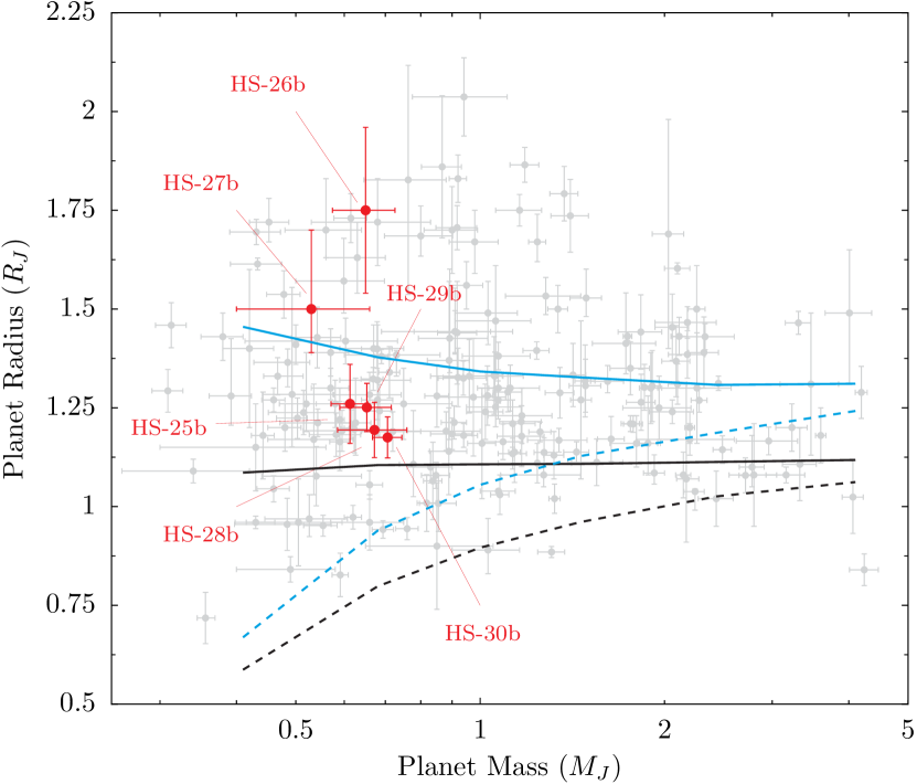
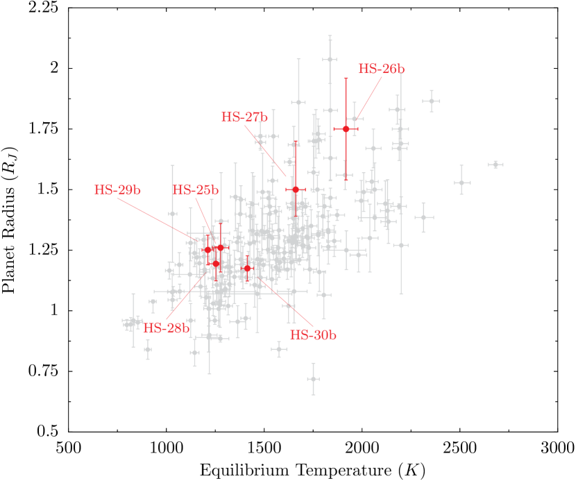
Figure 9.— (Left) Mass-radius diagram for all the transiting hot Jupiters discovered to date (grey points). Red points indicate the discovered exoplanets presented in this work. The black lines show the mass-radius relations of $4.5$ Gyr old planets at $0.045$ AU from the Sun obtained from Fortney et al. (2007) for core-free giant planets (solid line) and for planets with $100M_{\earth}$ cores (dashed line), which are appropriate for the insolation levels received by HATS-25b, HATS-28b, HATS-29b and HATS-30b. The blue lines show the same relations but for planets at $0.02$ AU, more (but not exactly) appropriate for the insolation levels received by HATS-26b and HATS-27b. We note, however, that these relations imply insolation levels around $2500$ times the solar insolation level at Earth, while the actual insolation levels for HATS-26b and HATS-27b are closer to $2250$ and $1250$ times the solar flux at Earth, respectively. (Right) Equilibrium temperature-radius diagram for all the transiting hot Jupiters discovered to date along with the discovered exoplanets presented in this work with the same colors as in the left plot.

The empirical relations in equation (9) of Enoch et al. (2012) predict the radii of these six new exoplanets to within the uncertainties. Therefore, these exoplanets appear to follow the trends followed by other close-in exoplanets, namely, that both increasing their semi-major axes and the effective temperatures leads to an increase in planetary radii. To further illustrate this, the right panel of Figure 9 shows the equilibrium temperature-radius diagram for the same exoplanets as on the left plot. We can clearly see that the correlation followed by most of the discovered transiting hot Jupiters to date is also followed by our newly discovered exoplanets.

In terms of future characterization, all the presented planets (except HATS-27b) have expected transmission signals between $\sim 700-900$ ppm and all (except HATS-28) have magnitudes between $V\sim 12-13$, making them interesting targets for future atmospheric studies. Figure 10 illustrates $V$ band magnitude versus the expected transmission signals for our newly discovered planets along with planets discovered to date, where the formula used to calculate the signal assumes an atmosphere that is five scale-heights thick, and is given by

$$\delta_{\textnormal{transpec}}=\frac{10R_{p}H}{R_{*}^{2}},$$

where $R_{p}$ is the planetary radius, $R_{*}$ is the stellar radius and $H=k_{B}T_{p}/mg_{p}$ is the planetary scale-height, calculated using Boltzmann’s constant, $k_{B}$, the planetary equilibrium temperature, $T_{p}$, the mean mass of the constituents that make up the atmosphere of the planet (assumed to be $\textnormal{H}_{2}$), $m$, and the acceleration due to gravity on the planetary surface, $g_{p}$. Systems already characterized by transmission spectroscopy are indicated in blue. As can be seen, the discovered exoplanets add to the increasing fraction of planets that have expected transmission signals on the same order as those already characterized. The most interesting systems in this respect are HATS-26b ($V=12.9$), which has an expected transmission signal of $\sim 900$ ppm and a long transit duration of $5.2$ hours, and HATS-29b ($V=12.6$), which has an expected transmission signal of $\sim 700$ ppm, a transit depth two times that of HATS-26b and a transit duration of $3.2$ hours.

Although not a good target for transmission, HATS-27b ($V=12.8$) is an attractive system if one is interested in estimating the projected spin-orbit alignment of the system: despite its modest planet-to-star ratio of ($R_{p}/R_{*}=0.0895\pm 0.0041$), the host star rotates at a moderately high rate ($v\sin(i)$ of $9.32\pm 0.5$ km/s) which, coupled with the long transit duration of $4.8$ hours, makes this inflated hot Jupiter a good target for follow-up Rossiter-McLaughlin (RM) observations. In particular, using equation (6) of Gaudi & Winn (2007), the amplitude of the RM effect, $K_{R}$, should be $\approx 75$ m/s. We obtained a precision of $\sim 30$ m/s in 10 minute exposures with HARPS for this star, making the RM effect readily detectable. In addition, given that the temperature of the host star is $6428\pm 64$ K, the system lies in a very interesting regime at which it has been claimed that planetary orbits of hot Jupiters shift from aligned to misaligned (Albrecht et al., 2012; Addison et al., 2016).

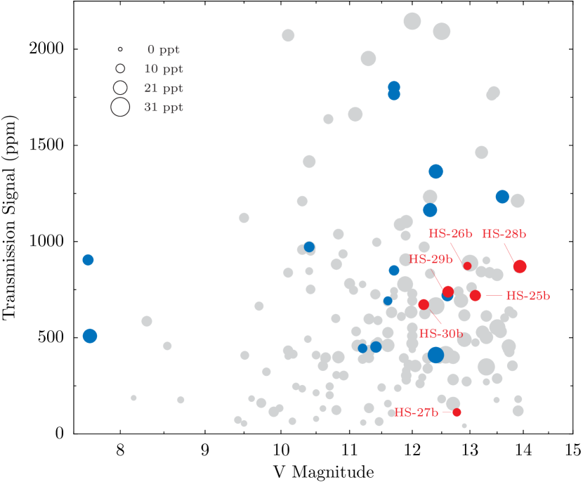
Figure 10.— Visual magnitude versus expected transmission signal for all the hot Jupiters discovered to date (grey points). Blue points indicate systems that have already been characterised via transmission spectroscopy, while red points indicate the exoplanets presented in this work. The size of the points indicate the transit depth with larger points indicating larger transit depths; the legend in the upper left corner indicates the corresponding depths in parts per thousand (ppt).

Table 8 Relative radial velocities and bisector spans for HATS-25–HATS-30.

Star	BJD	RV	$\sigma_{\rm RV}$	BS	$\sigma_{\rm BS}$	Phase	Instrument
	(2,450,000$+$)	($\rm m\,s^{-1}$)	($\rm m\,s^{-1}$)	($\rm m\,s^{-1}$)	($\rm m\,s^{-1}$)
HATS-25
HATS-25	$7067.85231$	$34.25$	$10.00$	$-19.0$	$40.0$	$0.941$	HARPS
HATS-25	$7067.87380$	$4.25$	$11.00$	$-2.0$	$40.0$	$0.946$	HARPS
HATS-25	$7068.86477$	$-70.75$	$7.00$	$-38.0$	$28.0$	$0.176$	HARPS
HATS-25	$7070.85785$	$57.25$	$9.00$	$-27.0$	$32.0$	$0.640$	HARPS
HATS-25	$7071.87936$	$54.25$	$21.00$	$15.0$	$70.0$	$0.878$	HARPS
HATS-25	$7072.88746$	$-48.75$	$9.00$	$-23.0$	$36.0$	$0.112$	HARPS
HATS-25	$7118.73269$	$80.25$	$16.00$	$-36.0$	$50.0$	$0.777$	HARPS
HATS-25	$7120.73472$	$-77.75$	$11.00$	$-14.0$	$40.0$	$0.243$	HARPS
HATS-26
HATS-26	$6828.49681$	$-65.10$	$28.00$	$150.0$	$24.0$	$0.213$	Coralie
HATS-26	$6829.52934$	$2.90$	$30.00$	$80.0$	$26.0$	$0.526$	Coralie
HATS-26	$7031.72967$	$58.90$	$15.00$	$30.0$	$12.0$	$0.754$	FEROS
HATS-26	$7035.82606$	$34.90$	$16.00$	$68.0$	$13.0$	$0.995$	FEROS
HATS-26	$7037.84686$	$22.90$	$15.00$	$34.0$	$12.0$	$0.607$	FEROS
HATS-26	$7049.79153$	$-56.10$	$16.00$	$71.0$	$12.0$	$0.224$	FEROS
HATS-26	$7050.84666$	$-1.10$	$15.00$	$64.0$	$12.0$	$0.543$	FEROS
HATS-26	$7053.88112$	$-3.10$	$17.00$	$59.0$	$13.0$	$0.462$	FEROS
HATS-26	$7054.81498$	$97.90$	$14.00$	$32.0$	$11.0$	$0.745$	FEROS
HATS-26	$7056.81639$	$-65.10$	$17.00$	$69.0$	$13.0$	$0.351$	FEROS
HATS-26	$7067.70058$	$68.91$	$18.00$	$67.0$	$38.0$	$0.647$	HARPS
HATS-26	$7069.77078$	$-92.09$	$20.00$	$8.0$	$42.0$	$0.273$	HARPS
HATS-26	$7070.73942$	$41.91$	$18.00$	$92.0$	$38.0$	$0.567$	HARPS
HATS-26	$7072.71165$	$-72.09$	$16.00$	$28.0$	$34.0$	$0.164$	HARPS
HATS-27
HATS-27	$6828.57385$	$29.59$	$40.00$	$24.0$	$29.0$	$0.704$	Coralie
HATS-27	$6828.62287$	$154.59$	$41.00$	$107.0$	$29.0$	$0.715$	Coralie
HATS-27	$6829.58090$	$16.59$	$37.00$	$79.0$	$27.0$	$0.922$	Coralie
HATS-27	$6841.56122$	$50.37$	$21.00$	$14.0$	$14.0$	$0.505$	FEROS
HATS-27	$6842.51976$	$22.37$	$17.00$	$71.0$	$12.0$	$0.712$	FEROS
HATS-27	$6845.58436$	$-47.63$	$17.00$	$48.0$	$12.0$	$0.373$	FEROS
HATS-27	$6846.47434$	$30.37$	$26.00$	$-69.0$	$15.0$	$0.565$	FEROS
HATS-27	$6847.47811$	$28.37$	$14.00$	$24.0$	$10.0$	$0.781$	FEROS
HATS-27	$6850.59743$	$54.37$	$23.00$	$8.0$	$14.0$	$0.454$	FEROS
HATS-27	$6851.54418$	$-33.63$	$18.00$	$11.0$	$12.0$	$0.658$	FEROS
HATS-27	$6852.48123$	$-16.63$	$18.00$	$74.0$	$12.0$	$0.860$	FEROS
HATS-27	$6852.58575$	$63.37$	$22.00$	$56.0$	$14.0$	$0.883$	FEROS
HATS-27	$6854.49043$	$-92.63$	$20.00$	$48.0$	$13.0$	$0.293$	FEROS
HATS-27	$6855.47772$	$-37.63$	$15.00$	$99.0$	$11.0$	$0.506$	FEROS
HATS-27	$6856.49742$	$29.37$	$13.00$	$32.0$	$10.0$	$0.726$	FEROS
HATS-27	$7067.80560$	$-38.64$	$25.00$	$73.0$	$48.0$	$0.296$	HARPS
HATS-27	$7068.84310$	$-24.64$	$15.00$	$18.0$	$30.0$	$0.520$	HARPS
HATS-27	$7069.87176$	$74.36$	$24.00$	$-6.0$	$48.0$	$0.741$	HARPS
HATS-27	$7070.83755$	$-18.64$	$20.00$	$30.0$	$38.0$	$0.950$	HARPS
HATS-27	$7071.86649$	$-100.64$	$40.00$	$58.0$	$72.0$	$0.172$	HARPS
HATS-27	$7072.87384$	$-1.64$	$25.00$	$-29.0$	$48.0$	$0.389$	HARPS
HATS-27	$7118.60461$	$-45.64$	$23.00$	$247.0$	$44.0$	$0.251$	HARPS
HATS-27	$7119.69411$	$224.37$	$26.00$	$468.0$	$16.0$	$0.486$	FEROS
HATS-27	$7119.76445$	$68.37$	$16.00$	$147.0$	$11.0$	$0.501$	FEROS
HATS-27	$7120.70644$	$105.36$	$27.00$	$55.0$	$48.0$	$0.704$	HARPS
HATS-27	$7121.56784$	$33.37$	$15.00$	$100.0$	$11.0$	$0.890$	FEROS
HATS-27	$7466.59338$	$-6.64$	$33.00$	$27.0$	$48.0$	$0.296$	HARPS
HATS-27	$7467.57122$	$25.36$	$27.00$	$37.0$	$38.0$	$0.507$	HARPS
HATS-27	$7468.57169$	$62.36$	$27.00$	$47.0$	$38.0$	$0.723$	HARPS
HATS-28
HATS-28	$7181.60951$	$-138.64$	$18.00$	$-149.0$	$25.0$	$0.313$	FEROS
HATS-28	$7182.79396$	$124.36$	$22.00$	$25.0$	$30.0$	$0.686$	FEROS
HATS-28	$7183.58139$	$54.36$	$22.00$	$-35.0$	$30.0$	$0.933$	FEROS
HATS-28	$7184.65002$	$-21.64$	$22.00$	$72.0$	$30.0$	$0.269$	FEROS
HATS-28	$7187.76095$	$-58.64$	$15.00$	$-36.0$	$20.0$	$0.247$	FEROS
HATS-28	$7188.73064$	$58.36$	$14.00$	$-94.0$	$18.0$	$0.552$	FEROS
HATS-28	$7189.88679$	$86.36$	$13.00$	$-5.0$	$18.0$	$0.915$	FEROS
HATS-28	$7191.66177$	$-53.64$	$12.00$	$-33.0$	$16.0$	$0.473$	FEROS
HATS-28	$7192.67821$	$88.36$	$19.00$	$2.0$	$25.0$	$0.793$	FEROS
HATS-28	$7193.76250$	$-67.64$	$11.00$	$1.0$	$15.0$	$0.134$	FEROS
HATS-28	$7194.62609$	$-48.64$	$12.00$	$45.0$	$16.0$	$0.405$	FEROS
HATS-28	$7196.85775$	$-96.64$	$15.00$	$-38.0$	$20.0$	$0.107$	FEROS
HATS-28	$7218.71803$	$17.36$	$25.00$	$-13.0$	$34.0$	$0.979$	FEROS
HATS-28	$7220.77528$	$55.36$	$20.00$	$4.0$	$26.0$	$0.625$	FEROS
HATS-28	$7223.54993$	$-89.64$	$24.00$	$-25.0$	$32.0$	$0.498$	FEROS
HATS-28	$7224.55108$	$73.36$	$14.00$	$-46.0$	$19.0$	$0.812$	FEROS
HATS-28	$7227.52090$	$114.36$	$10.00$	$-46.0$	$14.0$	$0.746$	FEROS
HATS-28	$7230.76298$	$79.36$	$11.00$	$-35.0$	$16.0$	$0.765$	FEROS
HATS-29
HATS-29	$7118.83135$	$44.32$	$19.00$	$-66.0$	$60.0$	$0.862$	HARPS
HATS-29	$7119.83810$	$-26.68$	$12.00$	$-42.0$	$44.0$	$0.080$	HARPS
HATS-29	$7120.82811$	$-75.68$	$7.00$	$-41.0$	$28.0$	$0.295$	HARPS
HATS-29	$7149.24168$	$-72.08$	$16.80$	$\cdots$	$\cdots$	$0.464$	CYCLOPS
HATS-29	$7149.25763$	$-22.98$	$17.70$	$\cdots$	$\cdots$	$0.468$	CYCLOPS
HATS-29	$7149.27360$	$-11.78$	$7.20$	$\cdots$	$\cdots$	$0.471$	CYCLOPS
HATS-29	$7150.27180$	$96.82$	$16.30$	$\cdots$	$\cdots$	$0.688$	CYCLOPS
HATS-29	$7150.28776$	$11.02$	$17.20$	$\cdots$	$\cdots$	$0.691$	CYCLOPS
HATS-29	$7150.30372$	$127.52$	$12.80$	$\cdots$	$\cdots$	$0.695$	CYCLOPS
HATS-29	$7152.13921$	$-1.98$	$9.70$	$\cdots$	$\cdots$	$0.093$	CYCLOPS
HATS-29	$7152.15453$	$-36.58$	$8.00$	$\cdots$	$\cdots$	$0.097$	CYCLOPS
HATS-29	$7152.16986$	$-15.58$	$11.00$	$\cdots$	$\cdots$	$0.100$	CYCLOPS
HATS-29	$7179.75812$	$-28.10$	$15.00$	$12.0$	$26.0$	$0.090$	Coralie
HATS-29	$7180.75107$	$-88.10$	$16.00$	$92.0$	$29.0$	$0.305$	Coralie
HATS-29	$7181.76069$	$13.90$	$13.00$	$-15.0$	$24.0$	$0.525$	Coralie
HATS-29	$7182.73909$	$87.90$	$14.00$	$-73.0$	$26.0$	$0.737$	Coralie
HATS-30
HATS-30	$6932.62878$	$-59.90$	$10.00$	$4.0$	$11.0$	$0.411$	FEROS
HATS-30	$6939.66985$	$86.61$	$15.00$	$-10.0$	$19.0$	$0.629$	Coralie
HATS-30	$6940.55468$	$31.61$	$14.00$	$-5.0$	$18.0$	$0.908$	Coralie
HATS-30	$6941.71844$	$-64.39$	$15.00$	$23.0$	$21.0$	$0.274$	Coralie
HATS-30	$6968.73018$	$70.61$	$12.00$	$-43.0$	$15.0$	$0.784$	Coralie
HATS-30	$6970.67182$	$-57.39$	$15.00$	$-77.0$	$19.0$	$0.395$	Coralie
HATS-30	$6972.60936$	$-27.39$	$14.00$	$-1.0$	$19.0$	$0.006$	Coralie
HATS-30	$6982.70613$	$-83.90$	$10.00$	$19.0$	$11.0$	$0.186$	FEROS
HATS-30	$6984.64881$	$89.10$	$10.00$	$34.0$	$11.0$	$0.798$	FEROS
HATS-30	$6985.58892$	$-49.90$	$10.00$	$29.0$	$11.0$	$0.095$	FEROS
HATS-30	$6997.56102$	$67.10$	$11.00$	$-12.0$	$13.0$	$0.866$	FEROS
HATS-30	$6998.61894$	$-97.90$	$10.00$	$13.0$	$10.0$	$0.199$	FEROS
HATS-30	$6999.66282$	$31.10$	$10.00$	$-8.0$	$11.0$	$0.528$	FEROS

References

- Addison et al. (2016) Addison, B. C., Tinney, C. G., Wright, D. J., & Bayliss, D. 2016, ArXiv e-prints, 1603.05754
- Addison et al. (2013) Addison, B. C., Tinney, C. G., Wright, D. J., et al. 2013, ApJ, 774, L9
- Albrecht et al. (2012) Albrecht, S., Winn, J. N., Johnson, J. A., et al. 2012, ApJ, 757, 18
- Bakos et al. (2010) Bakos, G. Á., Torres, G., Pál, A., et al. 2010, ApJ, 710, 1724
- Bakos et al. (2013) Bakos, G. Á., Csubry, Z., Penev, K., et al. 2013, PASP, 125, 154
- Baraffe et al. (2003) Baraffe, I., Chabrier, G., Barman, T. S., Allard, F., & Hauschildt, P. H. 2003, A&A, 402, 701
- Batygin & Stevenson (2010) Batygin, K., & Stevenson, D. J. 2010, ApJ, 714, L238
- Batygin et al. (2011) Batygin, K., Stevenson, D. J., & Bodenheimer, P. H. 2011, ApJ, 738, 1
- Bayliss et al. (2013) Bayliss, D., Zhou, G., Penev, K., et al. 2013, AJ, 146, 113
- Bayliss et al. (2015) Bayliss, D., Hartman, J. D., Bakos, G. Á., et al. 2015, AJ, 150, 49
- Benneke (2015) Benneke, B. 2015, ArXiv e-prints, 1504.07655
- Brown et al. (2013) Brown, T. M., Baliber, N., Bianco, F. B., et al. 2013, PASP, 125, 1031
- Burrows et al. (2007) Burrows, A., Hubeny, I., Budaj, J., & Hubbard, W. B. 2007, ApJ, 661, 502
- Cardelli et al. (1989) Cardelli, J. A., Clayton, G. C., & Mathis, J. S. 1989, ApJ, 345, 245
- Charbonneau et al. (2000) Charbonneau, D., Brown, T. M., Latham, D. W., & Mayor, M. 2000, ApJ, 529, L45
- Claret (2004) Claret, A. 2004, A&A, 428, 1001
- Crossfield (2015) Crossfield, I. J. M. 2015, PASP, 127, 941
- Dopita et al. (2007) Dopita, M., Hart, J., McGregor, P., et al. 2007, Ap&SS, 310, 255
- Enoch et al. (2012) Enoch, B., Collier Cameron, A., & Horne, K. 2012, A&A, 540, A99
- Fabrycky & Tremaine (2007) Fabrycky, D., & Tremaine, S. 2007, ApJ, 669, 1298
- Fortney et al. (2007) Fortney, J. J., Marley, M. S., & Barnes, J. W. 2007, ApJ, 659, 1661
- Fruchter & Hook (2002) Fruchter, A. S., & Hook, R. N. 2002, PASP, 114, 144
- Gaudi & Winn (2007) Gaudi, B. S., & Winn, J. N. 2007, ApJ, 655, 550
- Girardi et al. (2000) Girardi, L., Bressan, A., Bertelli, G., & Chiosi, C. 2000, A&AS, 141, 371
- Goldreich & Tremaine (1980) Goldreich, P., & Tremaine, S. 1980, ApJ, 241, 425
- Hansen & Barman (2007) Hansen, B. M. S., & Barman, T. 2007, ApJ, 671, 861
- Hartman et al. (2012) Hartman, J. D., Bakos, G. Á., Béky, B., et al. 2012, AJ, 144, 139
- Hartman et al. (2015) Hartman, J. D., Bayliss, D., Brahm, R., et al. 2015, AJ, 149, 166
- Henry et al. (2000) Henry, G. W., Marcy, G. W., Butler, R. P., & Vogt, S. S. 2000, ApJ, 529, L41
- Hippler et al. (2009) Hippler, S., Bergfors, C., Brandner Wolfgang, et al. 2009, The Messenger, 137, 14
- Huang & Cumming (2012) Huang, X., & Cumming, A. 2012, ApJ, 757, 47
- Jordán et al. (2014) Jordán, A., Brahm, R., Bakos, G. Á., et al. 2014, AJ, 148, 29
- Kataria et al. (2016) Kataria, T., Sing, D. K., Lewis, N. K., et al. 2016, ArXiv e-prints, 1602.06733
- Kaufer & Pasquini (1998) Kaufer, A., & Pasquini, L. 1998, in Society of Photo-Optical Instrumentation Engineers (SPIE) Conference Series, Vol. 3355, Optical Astronomical Instrumentation, ed. S. D’Odorico, 844–854
- Kislyakova et al. (2014) Kislyakova, K. G., Holmström, M., Lammer, H., Odert, P., & Khodachenko, M. L. 2014, Science, 346, 981
- Kovács et al. (2002) Kovács, G., Zucker, S., & Mazeh, T. 2002, A&A, 391, 369
- Lissauer & Stevenson (2007) Lissauer, J. J., & Stevenson, D. J. 2007, Protostars and Planets V, 591
- Louden & Wheatley (2015) Louden, T., & Wheatley, P. J. 2015, ApJ, 814, L24
- Madhusudhan et al. (2014) Madhusudhan, N., Amin, M. A., & Kennedy, G. M. 2014, ApJ, 794, L12
- Mandel & Agol (2002) Mandel, K., & Agol, E. 2002, ApJ, 580, L171
- Mayor et al. (2003) Mayor, M., Pepe, F., Queloz, D., et al. 2003, The Messenger, 114, 20
- Ohta et al. (2005) Ohta, Y., Taruya, A., & Suto, Y. 2005, ApJ, 622, 1118
- Pál et al. (2008) Pál, A., Bakos, G. Á., Torres, G., et al. 2008, ApJ, 680, 1450
- Perna et al. (2010) Perna, R., Menou, K., & Rauscher, E. 2010, ApJ, 724, 313
- Petrovich (2015) Petrovich, C. 2015, ApJ, 805, 75
- Queloz et al. (2000) Queloz, D., Eggenberger, A., Mayor, M., et al. 2000, A&A, 359, L13
- Queloz et al. (2001) Queloz, D., Mayor, M., Udry, S., et al. 2001, The Messenger, 105, 1
- Rasio & Ford (1996) Rasio, F. A., & Ford, E. B. 1996, Science, 274, 954
- Sing et al. (2016) Sing, D. K., Fortney, J. J., Nikolov, N., et al. 2016, Nature, 529, 59
- Sozzetti et al. (2007) Sozzetti, A., Torres, G., Charbonneau, D., et al. 2007, ApJ, 664, 1190
- Spiegel & Burrows (2013) Spiegel, D. S., & Burrows, A. 2013, ApJ, 772, 76
- Winn (2007) Winn, J. N. 2007, in Astronomical Society of the Pacific Conference Series, Vol. 366, Transiting Extrapolar Planets Workshop, ed. C. Afonso, D. Weldrake, & T. Henning, 170
- Wu & Lithwick (2011) Wu, Y., & Lithwick, Y. 2011, ApJ, 735, 109
- Wu & Lithwick (2013) —. 2013, ApJ, 763, 13
- Yi et al. (2001) Yi, S., Demarque, P., Kim, Y.-C., et al. 2001, ApJS, 136, 417
- Zacharias et al. (2012) Zacharias, N., Finch, C. T., Girard, T. M., et al. 2012, VizieR Online Data Catalog, 1322, 0
- Zechmeister & Kürster (2009) Zechmeister, M., & Kürster, M. 2009, A&A, 496, 577
- Zhou et al. (2014) Zhou, G., Bayliss, D., Penev, K., et al. 2014, ArXiv e-prints, 1401.1582