Transport in Out-of-Equilibrium XXZ Chains: Exact Profiles of Charges and Currents
Abstract
We consider the non-equilibrium time evolution of piecewise homogeneous states in the XXZ spin- chain, a paradigmatic example of an interacting integrable model. The initial state can be thought as the result of joining chains with different global properties. Through dephasing, at late times the state becomes locally equivalent to a stationary state which explicitly depends on position and time. We propose a kinetic theory of elementary excitations and derive a continuity equation which fully characterizes the thermodynamics of the model. We restrict ourselves to the gapless phase and consider cases where the chains are prepared: 1) at different temperatures; 2) in the ground state of two different models; 3) in the “domain wall” state. We find excellent agreement (any discrepancy is within the numerical error) between theoretical predictions and numerical simulations of time evolution based on tebd algorithms. As a corollary, we unveil an exact expression for the expectation values of the charge currents in a generic stationary state.
During the last decade, the study of non-equilibrium dynamics in quantum many-body systems has experienced a golden age. The experimental possibility for investigating almost purely unitary time evolution exp sparked off a diffuse theoretical excitement EF:review ; P:review ; quench ; GE15 ; dephasing ; IlievskiPRLQL . The challenge was to understand in which sense unitarily evolving systems can relax to stationary states, and, if this happens, how to determine the stationary values of the observables. The main focus has been on translationally invariant systems. There, a clear theoretical construction has been developed: while the full system can not relax, in the thermodynamic limit finite subsystems can, as the rest of the system acts as an unusual bath. It was argued that the stationary values of local observables are determined by local and quasi-local conservation laws Doyon ; P:review ; EF:review . It is then convenient to distinguish between generic models, where the Hamiltonian is the only local conserved quantity, and integrable models, where the number of local charges scales with the systems’s size. It was conjectured that in the former case stationary values of local observables are described by Gibbs ensembles (ge) thermalization while in the latter by so-called generalised Gibbs ensembles (gge) Rigol07 . Importantly, traces of the underlying integrability remain even in the presence of small integrability-breaking perturbations: at intermediate times the expectation values of local observables approach quasi-stationary plateaux retaining infinite memory of the initial state prethermalization ; prerelaxation ; LGS:review ; prethermalizationexp .
In the absence of translational invariance the situation gets more complicated. In this context a variety of different settings have been considered, which can be cast into two main classes. The first consists of dynamics governed by translationally invariant Hamiltonians on inhomogeneous states. Relevant examples are the sudden junction of two chains at different temperature thermoelectricengine ; BD:review ; VM:review ; twotemperatures ; conjTT ; Zotos ; CAD:hydro ; 2Delta , with different magnetizations Antal ; twomagnetizations , or with other different global properties otherdifferentglobalproperties ; XXlqss . In the second class we include dynamics where the Hamiltonian features a localised defect Fdefect ; BF:NESSdef ; SM:toc ; CVZ:14 . In both cases, a non-equilibrium steady state (ness) emerges: around the junction of the chains in the first class of problems Ruelle ; BD:nessCFT ; CAD:hydro and close to the defect in the second Fdefect ; BF:NESSdef . The characterization of the transport properties of the ness have attracted tremendous attention; however, the ness is just the tip of the iceberg. In the limit of large time and large distance from the inhomogeneity, the state becomes locally equivalent to a nontrivial stationary state, which, in integrable models, turns out to depend only on the “ray” Antal ; BF:NESSdef ; XXlqss . We will refer to the latter as a locally-quasi-stationary state (lqss) BF:NESSdef . We note that ray-dependent profiles of specific observables emerge naturally in hydrodynamical approaches A:hydro , which have been applied also in more generic systems profilesgenericmodels . Even though these problems have been under scrutiny for a long time, exact analytic results have been obtained only in noninteracting models and conformal field theories, the role of interaction remaining elusive until now.
In this Letter we study transport phenomena in interacting integrable models, focusing on the first class of protocols. We propose a “kinetic theory” of the elementary excitations and obtain a continuity equation whose solution gives the exact lqss characterizing the state of the system at late times. Solving the continuity equation gives us full access to the state and, in particular, to the expectation values of charge densities and related currents in the entire light cone. To illustrate our ideas, we use the paradigmatic example of the XXZ model.
The model.
We consider the XXZ spin- chain described by the Hamiltonian
| (1) |
where is the chain’s length, bold symbols indicate quantum operators, and are spins . We consider , parametrise the anisotropy as and set . The model is solved by the Bethe ansatz Bethe : every eigenstate is parametrised by a set of complex “rapidities” fulfilling the Bethe equations
| (2) |
Following the “string hypothesis” Takahashibook , as the solutions to (2) are organised in different types of “string” patterns, composed by a set of rapidities with the same real part and equidistant imaginary parts. The different string types are interpreted as different species of quasi-particles with real rapidites. In the thermodynamic limit with fixed, the thermodynamic Bethe ansatz formalism (tba) applies; a thermodynamic state is parametrised by “particles” and “holes” distributions , one for each species of quasi-particles. These distributions, usually called “root densities”, are connected to one another through the thermodynamic version of (2), reported in SM . The number of species is finite when is a rational multiple of , which is the case considered in this paper. The expectation value of the density of a conserved charge in the stationary state reads as Korepinbook
| (3) |
where is the single-particle eigenvalue of the charge and is independent of the state. If is invariant under spin-flip , it is completely characterized by the expectation values of the local and quasi-local charges obtained from the unitary representations of the transfer matrix IlievskiPRLQL ; P:review . We indicate these charges by , with , and the single-particle eigenvalues by . The charges have an increasing typical range as a function of and ; in particular, are local Korepinbook and . We refer the reader to the Supplemental Material SM and to the specific literature Takahashibook ; Korepinbook ; P:review for further details. A case without spin-flip invariance is discussed in Example 3.
Locally-quasi-stationary state.
In integrable models, the information about an inhomogeneity spreads linearly in time because of stable quasi-particle excitations bonnes14 . These contribute to the emergence of non-trivial behavior along the rays . Dephasing mechanisms dephasing are active also in the inhomogeneous case so at sufficiently late times the dynamics are expected to slow down with an emergent timescale proportional to . Thus we assume that, for given , the expectation values of observables can be eventually described by a stationary state
| (4) |
Here acts non-trivially only around . The state is the lqss introduced in BF:NESSdef ; determining it exactly is our main goal.
Kinetic Theory.
Being stationary (for given ), is characterized by a set of root densities :
| (5) |
In particular, the charges can be written as in (3).
Since the root densities are fixed by the expectation values of the charges IlievskiPRLQL , the full lqss can be obtained by determining how their expectation values vary in time. We assume that the change is induced by the motion of elementary excitations and that the late time regime is characterized by a “dynamical equilibrium”, where the thermodynamic state varies only slightly even though a macroscopic number of quasi-particles is moving. The nature of quasi-particle excitations remains well defined while moving through the system; on the other hand, the excitation energy and the momentum depend on the macro-state bonnes14 , so the “mild” inhomogeneity of the lqss modifies the propagation velocity . This leads to
| (6) |
where is the charge density carried from to by the quasi-particles in the time interval . For given and , only excitations with velocity contribute to , namely
| (7) |
Here is the charge density transported by excitations with string type and rapidity . This quantity depends on through and will be expressed in terms of the root densities before long. Plugging (7) into (6) gives
| (8) |
By virtue of (3) we then find
| (9) |
The next step is to fix the form of in terms of the root densities. To this aim, it is convenient to consider an auxiliary toy problem as follows. Let a macroscopic subsystem be described by with all the root densities equal to zero except for , with and some small parameter. Let us then release the subsystem in the vacuum (), namely in an infinite bath of spins up . After a sufficiently long time it is reasonable to expect local relaxation to the vacuum. From (3) it follows that the total charge density flowed out of the subsystem reads . Crucially, we interpret this expression as the charge density associated with the quasi-particles of species and rapidity going out of the subsystem f:dr
| (10) |
Let us go back to the expression (9) and take (10) as the transported charge density; we find
| (11) |
Since is independent of , (11) is a continuity equation for the charge density and holds for any local and quasi-local charge . Using the completeness of the set we have
| (12) |
This is our main result: the root densities , characterizing the state, obey a continuity equation with a -dependent velocity, remarkable effect of the interaction that induces a state-dependent dressing on the elementary excitations. A priori, one would expect the physical picture based on a kinetic theory of excitations to be only approximately correct. In fact, we will provide evidence that (12) exactly describes the dynamics at late times and large distances along the ray .
Charge currents.
In a spin chain the current of a charge is defined through the following continuity equation
| (13) |
Imposing , this determines up to operators with zero expectation value in any translationally invariant state. In the infinite time limit along the ray the time-evolving state becomes homogeneous, so the expectation values of the currents are independent of their particular definitions. From (11) it follows
| (14) |
where is an arbitrary stationary state and the equivalence is up to a state-independent constant.
We now provide several compelling consistency checks for the validity of (14) and, in turn, of (11).
Check 1: Conservation of the energy current. In the XXZ model the energy current is equal to the second charge, namely: , where we introduced the notation . Using some tba identities one can easily show that this relation is satisfied by (14) SM .
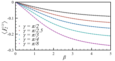
Check 2: Current(s) at equilibrium vs numerics. Fig. 1 shows the expectation value of the current in thermal states with inverse temperature and for different values of . The prediction (14) is checked against numerical data obtained using an algorithm based on the Matrix Product Density Operator (mpdo) representation of a mixed state SM . The agreement is unquestionably perfect: the discrepancies are smaller than the mpdo accuracy.
Determining the lqss.

We now turn to our main goal: the determination of the lqss evolving from an inhomogeneous state. We consider the time evolution of under the Hamiltonian (1) at sufficiently long times. The dynamics is described by (12), which, using some tba identities SM , can be recast in the form
| (15) |
where . Since , the solution is a piecewise constant function of . If, for any , has a unique solution note1 we find
| (16) |
Here is the step function which is nonzero and equal to only if . The functions and are the boundary conditions: due to the Lieb-Robinson bounds LR72 ; bravyi06 , there exists a maximal velocity such that observables on rays never receive information about the inhomogeneity; as a result, and describe the stationary states emerging independently in the two, left and right, bulk parts of the system (see also Fig. 3).
As depends on , (16) is only an implicit representation of the solution. In practice, one can solve the problem by iteration, starting from an initial , computing the excitation velocities, and iterating again until convergence is reached. The procedure is numerically very efficient and converges after few iterations.
Example 1: Two temperatures. Let us consider the transport problem par excellence: two chains prepared at different temperatures and then joined together BD:review .
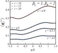
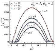
In Fig. 2 we report the rescaled profiles of a number of charges and currents for different times and interactions . The rescaled numerical data are in excellent agreement with the analytical predictions. This strongly suggests that the solution of (12) fully characterizes the state of the system at late times.
We note that at the edges of the light cone the predictions are not smooth, as the profiles are exactly flat outside the light cone. This is an infinite-time property, and indeed the numerical data are smooth at any time. Moreover, contrary to the noninteracting case, the velocities also depend on the temperatures bonnes14 , as revealed by the slight asymmetry of all the curves reported in Figs 2.
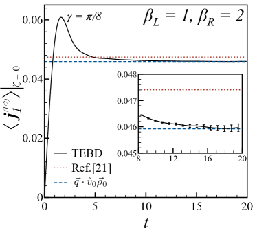
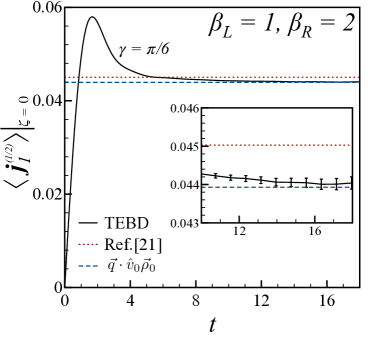
We mention that the conjecture put forward in Zotos for the energy current at is only in a fair agreement with our results SM .
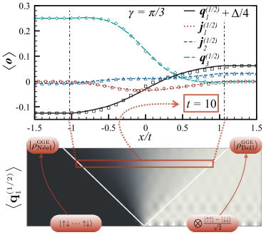
Example 2: Global quench. We now study the dynamics after joining together two globally different pure states which are not stationary. This is a genuine global quench with nontrivial time evolution also outside the light cone. As initial state we take the tensor product between the Néel state and the Bell state . As explained before, the two boundary conditions are the gge’s corresponding to the quenches and (see the down panel of Fig. 3). Relaxation is slower than in the first example and the comparison with the tebd data shown in Fig. 3 is jeopardised by the smallness of the time reached, consequence of the linear increase of the entropy both inside and outside the light cone. Nevertheless, the agreement is fairly good.
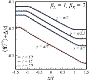
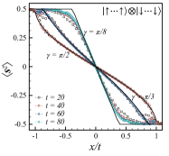
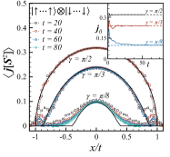
Example 3: Domain wall. If the initial state is not spin-flip invariant, the set is generally not sufficient to fix the state. First of all, one has to include the total spin along , , but also quasi-local charges coming from non-unitary representations of the transfer matrix P:review might play some role. Nonetheless, for a domain-wall initial state twomagnetizations , the comparison with numerics provides strong evidence that the expectation values of , , and the corresponding currents, can be obtained from the root densities solving the continuity equation (12). The left boundary condition is , while corresponds to the state in the limit . Fig. 4 shows the only two measured quantities exhibiting a non trivial behavior. Remarkably, the effective velocities of quasi-particles shrink to zero in the limit . A more careful analysis will be carried out in a future work.
Conclusions.
Using a “kinetic theory” of quasi-particles excitations, we derived a continuity equation (cf. (12)) describing the late time dynamics of the XXZ spin- chain after joining together two macroscopically different homogeneous states. We provided compelling evidence that equation (12) is in actual fact the exact continuity equation fulfilled by the conserved charges of the model for late times and large distances. We tested the predictions for the late-time dynamics against tebd numerical simulations and we have found excellent agreement. Our construction is sufficiently generic to be applicable to other interacting integrable models. In addition, the continuity equation can also be applied when integrability is broken by some localized inhomogeneity 2Delta : the solution of the late-time dynamics along the rays originating from the inhomogeneity is reduced to the determination of a few boundary conditions.
Acknowledgements.
We are very grateful to Lorenzo Piroli for the collaboration at an early stage of this project and for valuable comments on the manuscript. We thank Vincenzo Alba, Pasquale Calabrese, Ollala Castro-Alvaredo, Andrea De Luca, Jérôme Dubail, and Leonardo Mazza for useful discussions, Benjamin Doyon and Xenophon Zotos, also, for stimulating correspondence. This work was supported by the European Research Council under Starting Grant No. 279391 EDEQS (all authors), by the European Union’s Horizon 2020 research and innovation programme under the Marie Sklodowska-Curie Grant Agreement No. 701221 (M.C.), and by Laboratory of Excellence ENS-ICFP:ANR- 10-LABX-0010/ANR-10-IDEX-0001-02 PSL* (M.F., J.D.N.). J.D.N. and M.F. kindly acknowledge SISSA for the hospitality during the earlier stage of this work. Once this paper was being concluded, the preprint CAD:hydro appeared, where the same problem is independently studied for quantum field theories with diagonal scattering and a generalised hydrodynamical description is developed. In this framework, the authors derive an equation analogous to (12).References
- (1) M. Greiner et al, Nature 419, 51-54 (2002); T. Kinoshita, T. Wenger, and D. S. Weiss, Nature 440, 900 (2006); S. Hofferberth, I. Lesanovsky et al, Nature 449, 324-327 (2007); L. Hackermuller, U. Schneider et al, Science 327, 1621 (2010); S. Trotzky, Y.-A. Chen et al, Nature Phys. 8, 325 (2012); M. Gring, M. Kuhnert et al, Science 337, 1318 (2012): U. Schneider, L. Hackermüller et al, Nature Phys. 8, 213 (2012); M. Cheneau, P. Barmettler et al, Nature 481, 484 (2012); T. Langen, R. Geiger et al, Nature Physics 9, 640 (2013); F. Meinert, M.J. Mark et al, Phys. Rev. Lett. 111, 053003 (2013); T. Fukuhara, A. Kantian et al, Nature Physics 9, 235 (2013); T. Fukuhara, P. Schauß et al, Nature 502, 76 (2013); J.P. Ronzheimer, M. Schreiber et al, Phys. Rev. Lett. 110, 205301 (2013); P. Jurcevic, B. P. Lanyon et al, Nature 511, 202 (2014).
- (2) F.H.L. Essler and M. Fagotti, J. Stat. Mech. (2016) 064002.
- (3) C. Gogolin and J. Eisert, Rep. Prog. Phys. 79, 056001 (2016).
- (4) E. Ilievski, M. Medenjak et al, J. Stat. Mech. (2016) 064008; E. Ilievski, M. Medenjak, and T. Prosen, Phys. Rev. Lett. 115, 120601 (2015).
- (5) T. Barthel and U. Schollwöck, Phys. Rev. Lett. 100, 100601 (2008).
- (6) M. Rigol, A. Muramatsu, and M. Olshanii, Phys. Rev. A 74, 053616 (2006); M. A. Cazalilla, Phys. Rev. Lett. 97, 156403 (2006); P. Calabrese and J. Cardy, J. Stat. Mech. (2007) P06008; M. Cramer, C. M. Dawson, J. Eisert, and T. J. Osborne, Phys. Rev. Lett. 100, 030602 (2008); A. Silva, Phys. Rev. Lett. 101, 120603 (2008); P. Calabrese, F. H. L. Essler and M. Fagotti, Phys. Rev. Lett. 106, 227203 (2011); M. Fagotti and F.H.L. Essler, Phys. Rev. B 87, 245107 (2013); J.-S. Caux and R. M. Konik, Phys. Rev. Lett. 109, 175301 (2012); F. H. L. Essler, S. Evangelisti, and M. Fagotti, Phys. Rev. Lett. 109, 247206 (2012); M. Collura, S. Sotiriadis, and P. Calabrese, Phys. Rev. Lett. 110, 245301 (2013); J.-S. Caux and F.H.L. Essler, Phys. Rev. Lett. 110, 257203 (2013); G. Mussardo, Phys. Rev. Lett. 111, 100401 (2013); B. Pozsgay, J. Stat. Mech. (2013) P07003; M. Fagotti and F. H. L. Essler, J. Stat. Mech. (2013) P07012; W. Liu and N. Andrei, Phys. Rev. Lett. 112, 257204 (2014); J. De Nardis, B. Wouters, M. Brockmann, and J.-S. Caux, Phys. Rev. A 89, 033601 (2014); M. Fagotti, M. Collura et al, Phys. Rev. B 89, 125101 (2014); B. Wouters, J. De Nardis et al, Phys. Rev. Lett. 113, 117202 (2014); B. Pozsgay, M. Mestyán et al, Phys. Rev. Lett. 113, 117203 (2014); S. Sotiriadis and P. Calabrese, J. Stat. Mech. (2014) P07024; G. Goldstein and N. Andrei, Phys. Rev. A 90, 043625 (2014); F. H. L. Essler, G. Mussardo, and M. Panfil, Phys. Rev. A 91, 051602(R); L. Piroli, P. Calabrese, F.H.L. Essler, Phys. Rev. Lett. 116, 070408 (2016); B. Bertini, L. Piroli, P. Calabrese, J. Stat. Mech. (2016) 063102.
- (7) E. Ilievski, J. De Nardis, B. Wouters, J-S Caux, F. H. L. Essler, T. Prosen Phys. Rev. Lett. 115, 157201 (2015); E. Ilievski, E. Quinn, J. De Nardis, M. Brockmann arXiv:1512.04454 (2015).
- (8) B. Doyon, arXiv:1512.03713 (2015).
- (9) J. M. Deutsch, Phys. Rev. A 43, 2046 (1991); M. Srednicki, Phys. Rev. E 50, 888 (1994); M. Rigol, V. Dunjko, and M. Olshanii, Nature 452, 854 (2008); M. Rigol and M. Srednicki, Phys. Rev. Lett. 108, 110601 (2012).
- (10) M. Rigol, V. Dunjko, V. Yurovsky, and M. Olshanii, Phys. Rev. Lett. 98, 050405 (2007).
- (11) C. Kollath, A. M. Läuchli, and E. Altman, Phys. Rev. Lett. 98, 180601 (2007); M. Moeckel and S. Kehrein, Phys. Rev. Lett. 100, 175702 (2008); Ann. of Phys. 324, 2146 (2009); M. Kollar, F.A. Wolf, and M. Eckstein, Phys. Rev. B 84, 054304 (2011); M. Stark and M. Kollar, arXiv:1308.1610 (2013); M. Marcuzzi, J. Marino et al, Phys. Rev. Lett. 111, 197203 (2013); A. Mitra, Phys. Rev. B 87, 205109 (2013); F.H.L. Essler, S. Kehrein et al, Phys. Rev. B 89, 165104 (2014); A. Chiocchetta, M. Tavora et al, Phys. Rev. B 91, 220302(R) (2015); Erratum Phys. Rev. B 92, 219901(E) (2015); B. Bertini, F.H.L. Essler et al, Phys. Rev. Lett. 115, 180601 (2015); G.P. Brandino, J.-S. Caux, and R.M. Konik, Phys. Rev. X 5, 041043 (2015); M. Babadi, E. Demler, and M. Knap, Phys. Rev. X 5, 041005 (2015); N. Nessi and A. Iucci, arXiv:1503.02507 (2015).
- (12) M. Fagotti, J. Stat. Mech. (2014) P03016; B. Bertini and M. Fagotti, J. Stat. Mech. (2015) P07012; M. Fagotti and M. Collura, arXiv:1507.02678 (2015).
- (13) T. Langen, T. Gasenzer, and J. Schmiedmayer, J. Stat. Mech. (2016) 064009.
- (14) M. Gring, M. Kuhnert, et al, Science 14, 337 (2012); T. Langen, S. Erne et al, Science 348, 207 (2015).
- (15) J.-P. Brantut, C. Grenier, et al, Science 342, 713 (2013).
- (16) D. Bernard, B. Doyon, J. Stat. Mech. (2016) 064005.
- (17) R. Vasseur, J. E. Moore, J. Stat. Mech. (2016) 064010.
- (18) H. Spohn, J. L. Lebowitz, Comm. Math. Phys., 54, 97 (1977); T. Platini and D. Karevski, J. Phys. A: Math. Theor. 40 1711 (2007); W.H. Aschbacher and C.-A. Pillet, J. Stat. Phys. 112, 1153 (2003); W.H. Aschbacher and J.-M. Barbaroux, Lett. Math. Phys. 77, 11 (2006); D. Bernard and B. Doyon, J. Phys. A: Math. Theor. 45, 362001 (2012); M. Mintchev, J. Phys. A: Math. Theor. 44 415201 (2011). A. De Luca, J. Viti et al, Phys. Rev. B 88, 134301 (2013); C. Karrasch, R. Ilan, and J. E. Moore, Phys. Rev. B 88, 195129 (2013); M. Mintchev and P. Sorba, J. Phys. A: Math. Theor. 46, 095006 (2013); B. Doyon, M. Hoogeveen, and D. Bernard, J. Stat. Mech. (2014) P03002; V. Eisler, Z. Zimboras, New J. Phys. 16, 123020 (2014); M. Collura and D. Karevski, Phys. Rev. B 89 214308 (2014); M. Collura and G. Martelloni, J. Stat. Mech. (2014) P08006; A. De Luca, G. Martelloni, and J. Viti, Phys. Rev. A 91, 021603(R) (2015); B. Doyon, A. Lucas et al, J. Phys. A: Math. Theor. 48 095002 (2015); B. Doyon, Nucl. Phys. B 892, 190 (2015).
- (19) A. Biella, A. De Luca et al, Phys. Rev. B 93, 205121 (2016).
- (20) O. Castro-Alvaredo, Y. Chen et al, J. Stat. Mech. (2014) P03011; A. De Luca, J. Viti et al, Phys. Rev. B 90, 161101(R) (2014).
- (21) X. Zotos, arXiv:1604.08434 (2016).
- (22) O. A. Castro-Alvaredo, B. Doyon, and T. Yoshimura, arXiv:1605.07331 (2016).
- (23) T. Antal, Z. Racz et al, Phys. Rev. E 59, 4912 (1999).
- (24) T. Sabetta and G. Misguich, Phys. Rev. B 88, 245114 (2013); G. Goldstein and N. Andrei, arXiv:1309.3471 (2013); V. Alba and F. Heidrich-Meisner, Phys. Rev. B 90, 075144 (2014); E. Langmann, J. L. Lebowitz et al., Commun. Math. Phys. (2016), 1-32; L. Vidmar, D. Iyer, and M. Rigol, arXiv:1512.05373 (2015).
- (25) S. Sotiriadis and J. Cardy, J. Stat. Mech. P11003 (2008); P. Calabrese, C. Hagendorf, and P. Le Doussal, J. Stat. Mech. P07013 (2008); J. Lancaster and A. Mitra, Phys. Rev. E 81, 061134 (2010); V. Eisler and Z. Racz, Phys. Rev. Lett. 110, 060602 (2013).
- (26) J. Viti, J.-M. Stéphan et al, EPL 115 (2016) 40011; N. Allegra, J. Dubail et al., J. Stat. Mech. (2016) 053108.
- (27) M. Fagotti, arXiv:1508.04401 (2015).
- (28) M. Schirò and A. Mitra, Phys. Rev. Lett. 112, 246401 (2014).
- (29) C.-C. Chien, M. Di Ventra, M. Zwolak, Phys. Rev. A 90, 023624 (2014).
- (30) B. Bertini and M. Fagotti, Phys. Rev. Lett. 117, 130402 (2016).
- (31) D. Ruelle, J. Stat. Phys. 98, 57 (2000).
- (32) D. Bernard and B. Doyon, Ann. H. Poincaré 16, 113 (2015).
- (33) A. G. Abanov, in Applications of Random Matrices in Physics, Vol. 221 NATO Science Series II: Mathematics, Physics and Chemistry; A. G. Abanov and P. B. Wiegmann, Phys. Rev. Lett. 95, 076402 (2005).
- (34) M. J. Bhaseen, B. Doyon, et al., Nature Physics 11, 509 (2015); R. Pourhasan, High Energ. Phys. (2016) 2016: 5; A. Lucas, K. Schalm, et. al., Phys. Rev. D 94, 025004 (2016); M. Spillane, C. P. Herzog, arXiv:1512.09071 (2015).
- (35) H. Bethe, Z. Phys. 71, 205 (1931); R. Orbach, Phys. Rev. 112, 309 (1958).
- (36) M. Takahashi, Thermodynamics of One-dimensional Solvable Models (Cambridge University Press, 2005).
- (37) See the Supplemental Material.
- (38) V.E. Korepin, A.G. Izergin, and N.M. Bogoliubov, Quantum Inverse Scattering Method, Correlation Functions and Algebraic Bethe Ansatz (Cambridge University Press, 1993).
- (39) L. Bonnes, F.H.L. Essler and A. M. Läuchli, Phys. Rev. Lett. 113, 187203 (2014).
- (40) The reader familiar with the tba could wonder why this expression is not written in terms of dressed quantities. Essentially, this is because a macroscopic number of excitations is moving.
- (41) Note that has always an odd number of zeros, indeed the velocity is bounded and hence .
- (42) E. H. Lieb and D. W. Robinson, Commun. Math. Phys. 28, 251 (1972).
- (43) S. Bravyi, M. B. Hastings, and F. Verstraete, Phys. Rev. Lett. 97, 050401 (2006).
- (44) F. Verstraete, J. J. García-Ripoll, and J. I. Cirac, Phys. Rev. Lett. 93, 207204 (2004); M. Zwolak and G. Vidal, Phys. Rev. Lett. 93, 207205 (2004); A. H. Werner, D. Jaschke et al, Phys. Rev. Lett. 116, 237201 (2016).
- (45) G. Vidal, Phys. Rev. Lett. 93, 040502 (2004).
Supplemental Material for
“Transport in Out-of-Equilibrium XXZ Chains: Exact Profiles of Charges and Currents”
We collect here the technical tools used in the manuscript.
-
-
Section I presents the numerical method used to simulate the XXZ spin chain after a quantum quench from an inhomogeneous state.
-
-
Section II is a concise introduction to the thermodynamic Bethe Ansatz (tba) formalism, which is the one we adopted to work out our results. It does not aim at being a complete review of the tba and, for a more systematic description, we refer the reader to Takahashibook . Importantly, subsection II.1 explains the meaning of quasi-particle excitation on a thermodynamic Bethe state, which constitutes the key element of the kinetic theory introduced in the paper.
-
-
Section III derives the tba identities used in the main text.
-
-
Section IV reports additional examples where the initial state consists of two chains prepared at different temperatures and then joined together.
- -
I On the numerical simulations
Static and dynamical properties of the open XXZ spin- chain can be efficiently investigated using mps-based algorithms. The starting point is the matrix-product state representation of the initial state
| (17) |
Here is the length of the chain; the physical index runs over the local Hilbert space spanned by ; are matrices associated with the lattice site; are diagonal matrices with as entries the singular values corresponding to the bipartition of the system at the bond (namely between site and site ).
The representation (17) holds for pure states, but can be straightforwardly generalized to a mixed state MPDO . It reads as
| (18) |
Since the density matrix is positive semidefinite, the matrices in (18) can be decomposed as follows
| (19) |
where the index runs on a local auxiliary space with dimension . For a pure state, .
As a consequence of (18) and (19), any operation on mixed states can be reformulated using the standard mps language, as an operation on a locally purified state. In practice, an auxiliary system (ancilla) with local Hilbert space of dimension is associated with each local spin, allowing to write the locally purified mps state as
| (20) |
The original mixed state is obtained by tracing out the ancillas, namely . We note that for thermal states, which are the only mixed states we consider here, the local ancilla can be chosen to be a spin-, namely .
Using the representations (17) and (20), we implemented both real and imaginary time-evolution using the Time Evolving Block Decimation (tebd) procedure TEBD . Specifically, the (imaginary) time is discretized and we use the -order Suzuki-Trotter decomposition of the time-step evolution operator, with real time discretization , and imaginary time discretization (inverse-temperature step) .
For initial states that can be represented in terms of pure mps states (e.g. ), we only need the real-time evolution operator, which is given by
| (21) |
Here is the local XXZ Hamiltonian density.
For thermal states we implemented both real-time and imaginary-time evolution operators
| (22) | ||||
| (23) |
Here we defined and , where the operators on the left of the tensor product act on the physical spins and the ones on the right on the ancillas.
The imaginary-time evolution is used to construct thermal states at generic inverse temperature as follows. The infinite temperature state admits an exact mpdo representation with auxiliary dimension and . A mpdo representation of the finite temperature state at inverse temperature is then constructed by evolving in imaginary time up to inverse temperature : During the imaginary time evolution, remains fixed while the auxiliary dimension is dynamically updated by retaining all singular values larger than zero. This can be easily accomplished since the temperature introduces a finite correlation length and, in the range of temperatures considered, the mpdo description of the state is free from truncation errors. The only unavoidable source of error is the Suzuki-Trotter approximation, giving an error of the order .
We followed an analogous procedure also for the real-time evolution, updating the auxiliary dimension dynamically. However, we set a maximum auxiliary dimension depending on the post-quench value of . With this choice, in the time window explored (), the total error remains .
In the numerical implementation, we partially fixed the gauge freedom of the mps by imposing both the left and right canonical form; namely the tensors satisfy the following relations
| (24) |
with the identity matrix. As a consequence, the expectation value of any local quantity with support in the lattice interval (with ), is given by
| (25) |
where implicit summation over the repeated indices is understood.
I.1 Charges and currents
We implemented the charge densities:
| (26) |
| (27) |
| (28) |
| (29) |
and charge currents:
| (30) |
| (31) |
| (32) |
II Thermodynamic Bethe-ansatz for the XXZ spin- chain
The XXZ Hamiltonian can be diagonalized by Bethe Ansatz. We take the ferromagnetic state with all spins up as a reference state and build interacting spin waves as excitations over this state. A state with down spins has total magnetization given by and is characterized by a set of complex rapidities . It can be written as follows
| (33a) | |||
| where denotes the position of the -th down spin, and we ordered the sequence so that for . The wave function in coordinate space takes the Bethe Ansatz form | |||
| (33b) | |||
The sum runs over the set of all permutations of integers , denoted by , and is the parity of the permutation . The single particle momentum is given by
| (34) |
The parameter is such that . The scattering phase shift reads as
| (35) |
If the rapidities satisfy the Bethe equations,
| (36) |
the state (33) is an eigenstate of the Hamiltonian and is called a “Bethe state”. The solutions to the equations (36) are complex numbers which can be arranged in “strings”, i.e., they can be parametrized as follows Takahashibook :
| (37) |
Here denotes the number of the species of excitations, labels the species, is the length of the corresponding string, indexes the strings of a given species, and runs over the rapidities in the same string. The index is called “parity” and are the real string centers, which are representative of the real parts of the rapidities in the same string. For a given state, in most of the strings the deviations vanish exponentially with the system size . This is in accordance with the string hypothesis: for large enough , all the solutions of the Bethe equations are arranged in perfect strings (rapidities disposed as in (37) with zero deviations ); a state is then solely characterized by the real string centers . The logarithmic form of the Bethe Eqs (36) can be recast into the Bethe-Gaudin-Takahashi equations for string centers Takahashibook
| (38) |
where is integer, if the number of string centers of the -th species is odd, and half-integer, if is even. Note the numbers of string centers are such that
| (39) |
The dispersion kernels and scattering phases appearing here are
| (40) |
At the so-called “roots of unity” points the number of string types is
| (41) |
In the thermodynamic limit, for each string type the rapidities become dense on the real axis . Let us introduce the counting functions
| (42) |
These are monotonic functions such that
| (43) |
where are the solutions to (38). These relations can be used to establish a one to one correspondence between rapidities and integers
| (44) |
In particular, for a given solution of (38), (44) produces a corresponding set of integers, which we say to be occupied. The other integers corresponding through (44) to rapidities which do not appear in are said empty. Rapidities corresponding to occupied and empty integers are called particles and holes respectively. Since particles and holes become dense in the thermodynamic limit, one can recast the problem of finding their actual values into the determination of their “macroscopic” distributions and , defined as
| (45) |
These functions are called root densities and are related to the counting functions as follows
| (46) |
where
| (47) |
and is an auxiliary integer variable which will be defined later for the cases investigated.
For later reference, it is useful to introduce the following notation
| (48) |
In the thermodynamic limit, equations (38) involve both counting functions and root densities. The dependence on counting functions can be removed by differentiating and making use of (46); this leads to the so called tba equations
| (49) |
Here the sum over runs over all the string types and we introduced
| (50) | ||||
| (51) |
The distributions are normalized by the total number of particles, which is in a simple relation to the magnetization density
| (52) |
The energy density is instead given by
| (53) |
where is the energy of a string of type with rapidity , obtained by summing over all the contributions of the single particles inside the string
| (54) |
Equivalently, any other charge density of a thermodynamic state can be expressed in terms of the distribution of particles
| (55) |
where is the single particle eigenvalue and
| (56) |
II.1 Excitations over a generic thermodynamic state
A thermodynamic state can be defined as the thermodynamic limit of a single representative state specified by a set of quantum numbers which corresponds to a set of rapidities . At fixed string type , we can define excitations on top of this state, as displacements of some quantum numbers . We may then split the set of rapidities in “non-excited ones” , with , a set of particle excitations , and a set of hole excitations . The latter contains fictitious rapidities which represent the empty slots left by the particle excitations. The total number of excitations is assumed to be even. The rapidities in the first set are related to the ones of the representative state as follows
| (57) |
where is equal to () for particle (hole) excitations, is the number of excitations for given species , and is the so-called shift function satisfying the following integral equation
| (58) |
Given equation (57) we can then write down the corrections to the the energy of the state due to the presence of the particle-hole excitations
| (59) | ||||
| (60) |
The same computation can be carried out for the difference of momenta
| (61) | ||||
| (62) |
We can then define the energy and momenta for a single particle excitation with rapidity and string type as
| (63) |
| (64) |
These are the so-called dressed energy and momentum.
This analysis can be easily extended to all the other conserved charges of the model. It turns out that an excitation with rapidity and string type “carries” a dressed charge given by
| (65) |
Here is the single particle eigenvalue of .
II.2 Thermal states
A special class of thermodynamic Bethe states is given by the thermal states, which are equivalent to the following density matrix
| (66) |
Here is the inverse temperature and we introduced an external magnetic field along the direction.
The thermal states are defined by the following integral equations for the functions
| (67) |
Remarkably, for these states (and these states only) the dressed energy is related to the functions as
| (68) |
II.2.1 String content at
At the simple roots of unity points there are strings with the following lengths and parities
| (69) | ||||
| (70) |
In this case, the auxiliary integers (cf. (47)) read as
| (71) | ||||
| (72) |
II.2.2 String content at
The more involved case of has string types. Here we have:
| (73) | |||
| (74) | |||
| (75) |
III Proof of some identities
In this section we prove some useful identities. In doing that, it is convenient to introduce the following compact notations. Any function of the rapidities with a string index is represented by a vector
| (76) |
Any function of two rapidities with two string indices is instead represented by an operator acting as follows
| (77) |
The inverse of is the operator satisfying
| (78) |
Thus, the distribution corresponds to the identity . It is also convenient to define diagonal operators associated with a function of a single rapidity
| (79) |
Finally, the scalar product is defined as
| (80) |
III.1 Root density
In compact notations, the tba equations (49) read as
| (81) |
By definition, the root density is in a simple relation with :
| (82) |
We can therefore invert (81) to get
| (83) |
and, in turn, the root density
| (84) |
III.1.1 Expectation values of charge densities
Using (84), we can easily express the expectation value of a charge density (Eq. (3) in the main text) in terms of
| (85) |
III.2 Expectation values of charge currents
Let us rewrite (65) in compact notations
| (86) |
Here is the transpose of and is the shift function (cf. Eq.(58)). Inverting (58) we find
| (87) |
where . Plugging this into (86) gives
| (88) |
Considering the equation in “components” , differentiating with respect to and rewriting everything in compact notations, we get
| (89) |
By definition, the velocity of the elementary excitations is the derivative of the energy with respect to the momentum
| (90) |
Using (89) we have
| (91) |
in components it reads as
| (92) |
From this relation and (90) it follows
| (93) |
Applying (89) to the derivative of the excitation energy gives
| (94) |
and hence
| (95) |
Up to a constant, the current written in Eq. (14) of the main text is therefore given by
| (96) |
In particular, using and we have
| (97) |
where in the last step we used the symmetry of . Eq. (97) proves , as claimed in the main text.
III.2.1 Comparison with Ref. CAD:hydro
As mentioned in the main text, in Ref. CAD:hydro an exact expression for the expectation values of current densities was independently obtained for integrable quantum field theories with diagonal scattering. In our notations it reads as
| (98) |
where the subscript iqft stands for integrable quantum field theory and , , , and have meanings analogous to the corresponding quantities in XXZ. This expression is the integrable quantum field theory equivalent of (96) and, in fact, can be recast as in Eq. (14) of the main text.
III.3 Continuity equation
We are now in a position to prove Eq. (15) of the main text. Since , Eq. (12) can be rewritten as
| (99) |
Using the explicit expressions (84) and (95) for and we find
| (100) |
Since only depends on , the derivative of with respect to is readily obtained
| (101) |
Plugging this into (99) gives
| (102) |
This can be rewritten as
| (103) |
Since is invertible, this equation is equivalent to
| (104) |
which is exactly Eq. (15) of the main text.
An interesting corollary of (104) is that the continuity equation can be alternatively expressed in terms of the density of holes as follows
| (105) |
This is because the transformation mapping particles into holes maps into and the velocity in itself; the statement then follows from the invariance of (104) under such transformation.
IV Two temperatures quench: additional example
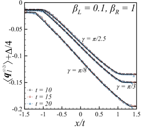
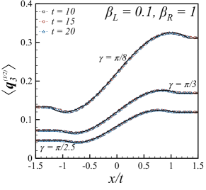
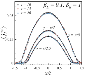
Here we consider an other example of time evolution after joining two chains at different temperature. In Fig. 5 we report the rescaled profiles of a number of charges and currents ( is the energy current) for different times and interactions in the case of and .
As shown in the figure, the rescaled numerical data are in excellent agreement with the analytical predictions. We note that the maximal velocities are smaller than in the case reported in Fig. 2 of the main text.

.
V Comparison with Ref. Zotos
In this section we compare our results with the conjecture of Ref. Zotos for the energy current at . In compact notations (cf. (76)–(80)), Ref. Zotos proposed
| (106) |
Here is the step function and where are thermal root densities (cf. (67)) at inverse temperature and respectively. In Table 1 we report a comparison between this conjecture and our result for the same observable, namely . We consider , the value of the anisotropy for which Ref. Zotos showed the best agreement with the numerical simulations. The differences found are appreciable but smaller than the accuracy of our tebd simulations, see Tab. 1. In order to distinguish between our prediction and the conjecture of Ref. Zotos , we considered larger values of . The discrepancy between the two results increases with and the numerical simulations corroborate the exactness of our prediction; see Fig. 6 for two representative examples.
| Ref. Zotos | ||
|---|---|---|
| 1 | 0.0191 | 0.0193 |
| 2 | 0.0318 | 0.0319 |
| 3 | 0.0335 | 0.0333 |
| 4 | 0.0294 | 0.0290 |
| 5 | 0.0241 | 0.0235 |
| 6 | 0.0192 | 0.0186 |
| 7 | 0.0153 | 0.0147 |
| 8 | 0.0123 | 0.0118 |
