Fast approximate furthest neighbors with data-dependent hashing

Abstract

We present a novel hashing strategy for approximate furthest neighbor search that selects projection bases using the data distribution. This strategy leads to an algorithm, which we call DrusillaHash, that is able to outperform existing approximate furthest neighbor strategies. Our strategy is motivated by an empirical study of the behavior of the furthest neighbor search problem, which lends intuition for where our algorithm is most useful. We also present a variant of the algorithm that gives an absolute approximation guarantee; to our knowledge, this is the first such approximate furthest neighbor hashing approach to give such a guarantee. Performance studies indicate that DrusillaHash can achieve comparable levels of approximation to other algorithms while giving up to an order of magnitude speedup. An implementation is available in the mlpack machine learning library (found at http://www.mlpack.org).

1 Introduction

We concern ourselves with the problem of furthest neighbor search, which is the logical opposite of the well-known problem of nearest neighbor search. Instead of finding the nearest neighbor of a query point, our goal is to find the furthest neighbor. This problem has applications in recommender systems, where furthest neighbors can increase the diversity of recommendations [1, 2]. Furthest neighbor search is also a component in some nonlinear dimensionality reduction algorithms [3], complete linkage clustering [4, 5] and other clustering applications [6]. Thus, being able to quickly return furthest neighbors is a significant practical concern for many applications.

However, it is in general not feasible to return exact furthest neighbors from large sets of points. Although this is possible with Voronoi diagrams in 2 or 3 dimensions [7], and with single-tree or dual-tree algorithms in higher dimensions [8], these algorithms tend to have long running times in practice. Therefore, approximate algorithms are often considered acceptable in most applications.

For approximate neighbor search algorithms, hashing strategies are a popular option [9, 10, 11]. Typically hashing has been applied to the problem of nearest neighbor search, but recently there has been interest in applying hashing techniques to furthest neighbor search [12, 13]. In general, these techniques are based on random projections, where random unit vectors are chosen as projection bases. This allows probabilistic error guarantees, but the entirely random approach does not use the structure of the dataset.

In this paper, we first consider the structure of the furthest neighbors problem and then conclude that a data-dependent approach can be used to select the projection bases for a hashing algorithm. This allows us to develop:

• DrusillaHash, a hashing algorithm that uses data-dependent projection bases and outperforms other approximate furthest neighbors approaches in practice.

• A modified version of DrusillaHash which satisfies rigorous approximation guarantees, though it is not likely to be useful in practice.

Our empirical results in Section 7 show that the DrusillaHash algorithm demonstrably outperforms existing solutions for approximate $k$-furthest-neighbor search.

2 Notation and formal problem description

The problem of furthest neighbor search is easily formalized. Given a set of reference points $S_{r}\in\mathcal{R}^{n\times d}$, a set of query points $S_{q}\in\mathcal{R}^{m\times d}$, and a distance metric $d(\cdot,\cdot)$, the problem is to find, for each query point $p_{q}\in S_{q}$,

$$\operatorname{argmax}_{p_{r}\in S_{r}}d(p_{q},p_{r}).$$ (1)

A trivial way to solve this algorithm is by brute-force: for each query point, loop over all reference points and find the furthest one. But this algorithm takes $O(nm)$ time, and does not scale well to large $S_{r}$ or $S_{q}$. In this paper, we will consider the $\epsilon$-approximate form of the furthest neighbor search problem.

Given a set of reference points $S_{r}\in\mathcal{R}^{n\times d}$, a set of query points $S_{q}\in\mathcal{R}^{m\times d}$, an approximation parameter $\epsilon\geq 0$, and a distance metric $d(\cdot,\cdot)$, the $\epsilon$-approximate furthest neighbor problem is to find a furthest neighbor candidate $\hat{p}_{fn}$ for each query point $p_{q}\in S_{q}$ such that

$$\frac{d(p_{q},p_{fn})}{d(p_{q},\hat{p}_{fn})}<1+\epsilon$$ (2)

where $p_{fn}$ is the true furthest neighbor of $p_{q}$ in $S_{r}$. When $\epsilon=0$, this reduces to the exact furthest neighbor search problem. This form of approximation is also known as relative-value approximation.

3 Related work

There have been a number of improvements over the naive brute-force search algorithm suggested above. Exact techniques based on Voronoi diagrams can solve the furthest neighbor problem. In 1981, Toussaint and Bhattacharya proposed building a furthest-point Voronoi diagram to solve the furthest neighbors problem in $O(m\log n)$ time [14]. But in high dimensions, Voronoi diagrams are not useful because of their exponential memory dependence on the dimension.

Another approach to exact furthest neighbor search uses space trees, as described by Curtin et al. [8]. A tree is built on the reference points $S_{r}$, and nodes that cannot contain the furthest neighbor of a given query point are pruned. This is essentially equivalent to many algorithms for nearest neighbor search, such as the algorithm for nearest neighbor search with cover trees [15], but with inequalities reversed (i.e., we prune nearby nodes instead of faraway nodes). It is also possible to do this in a dual-tree setting, by also building a tree on the query points $S_{q}$. Dual-tree nearest neighbor search has been proven to scale linearly in the size of the reference set under some conditions [16]; however, no similar bound has been shown for dual-tree furthest neighbor search. It would be reasonable to expect similar empirical scaling. Unfortunately, tree-based approaches tend to perform poorly in high dimensions, and the construction time of the trees can cause the algorithm to be slower than desirable in practice.

Further runtime acceleration can be achieved if approximation is allowed. It is easy to modify the single-tree and dual-tree algorithms to support this, in the manner suggested by Curtin for nearest neighbor search [17]. Although this is shown to accelerate nearest neighbor search runtime by a significant amount (depending on the allowed approximation), the setup time of building the trees can still dominate. A similar approach to this strategy is the fair split tree, designed by Bespamyatnikh [18]. But this approach suffers from the same issues.

The fastest known algorithms for approximate nearest neighbor search are hashing algorithms. Indyk [13] proposed a hashing algorithm based on random projections that is able to solve a slightly different problem: this algorithm is able to determine (approximately) whether or not there exists a point in $S_{r}$ farther away than a given distance. This can be reduced to the approximate furthest neighbor problem we are interested in, but this is complex to implement.

Pagh et al. [12] refine this approach in order to directly solve the approximate furthest neighbor problem; this improves on the runtime of Indyk’s algorithm and is easy to implement. This algorithm, called QDAFN (‘query-dependent approximate furthest neighbor’), has a guaranteed success probability. The algorithm is parameterized by the number of projections used and the number of points stored for each projection; usually, this number is relatively low. But in extremely high-dimensional settings, the randomly-chosen projections can fail to capture important outlying points. This motivates us to investigate the point distribution in order to choose projection bases.

4 Furthest neighbor point distribution

The furthest neighbor problem is significantly different from the nearest neighbor problem, which has received significantly more attention [19, 20, 21, 22, 9, 8, 17]. This difference is perhaps somewhat counterintuitive, given that the furthest neighbor problem is simply an $\operatorname{argmax}$ over all reference points instead of an $\operatorname{argmin}$. But this small change causes the problem to have surprisingly different structure with respect to the results.

As a first observation of the differences between the two problems, consider that for any set $S_{r}$, the furthest neighbor of every point can be made to be a single point simply by adding a single point sufficiently far from every other point in $S_{r}$. There is no analog to this in the nearest neighbor search problem. Indeed, it is often true that for a furthest neighbor query with many query points, the results may contain the same reference point. This is easily demonstrated.

Define the rank of a reference point $p_{r}$ for some query point $p_{q}$ as the position of $p_{r}$ in the ordered list of distances from $p_{q}$. That is, if the rank of $p_{r}$ for some query point $p_{q}$ is $k$, then $p_{r}$ is the $k$-furthest neighbor from $p_{q}$.

We can obtain insight into the behavior of furthest neighbor queries by observing the average rank of points on some example datasets from the UCI dataset repository [23]. Figure 1 contains scatterplots displaying the average rank of a reference point versus the mean-centered norm of the reference point for the all-furthest-neighbors problem (that is, each point in the reference set is used as a query point).

(a) cloud dataset (10x2047).

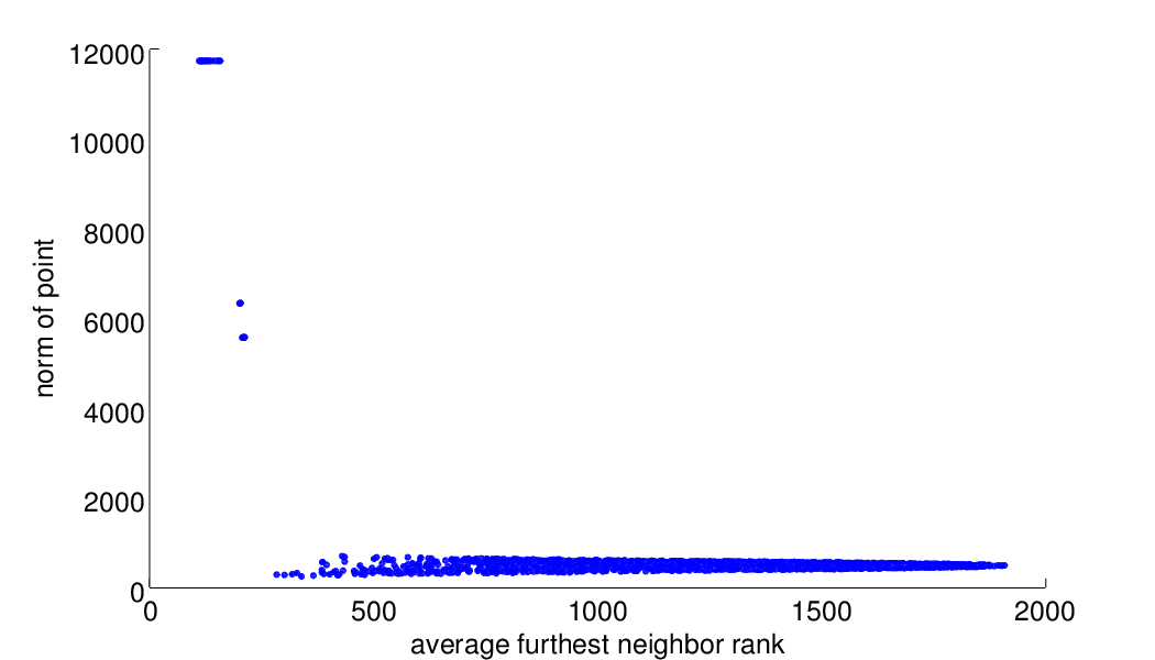
(b) ozone dataset (10x2047).

(c) phy dataset (78x150000).

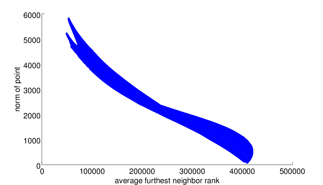
(d) covertype dataset (55x581012).

Figure 1: Average rank vs. norm for a handful of datasets. Observe that a large norm is correlated with a low rank.

Figure 1 shows that there is a clear and unmistakable correlation between the norm of a point and its average rank for the all-$k$-furthest-neighbor problem. For the ozone dataset, we can see that there are only a few points with high norm, and all of these have much lower average rank than the rest of the points.

These observations suggest that a reasonable approximate furthest neighbor algorithm might be obtained simply by searching over the top few points in the reference set with highest norm. Unfortunately, an algorithm that simple will fail in many cases in practice. Still, an effective furthest neighbors algorithm should take this structure into account: high-norm points are more important than low-norm points.

5 The algorithm: DrusillaHash

Figure 2: Distortion and offset for $p_{j}$ with base vector $v_{i}$.

Our collective observations motivate a hashing algorithm for approximate furthest neighbor search, which we introduce as DrusillaHash in Algorithm 1. The algorithm constructs hash tables by repeatedly choosing points currently not in any hash table with largest norm. After the hash tables are built, each query point is simply compared with all points in each hash table in order to determine a good furthest neighbor candidate.

1:  Input: reference set $S_{r}$, query set $S_{q}$, number of neighbors $k$, number of tables $l$, table size $m$

2:  Output: array of furthest neighbors $N[]$

3:  {Pre-processing: mean-center data.}

4:  $m\leftarrow\frac{1}{n}\sum_{p_{r}\in S_{r}}p_{r}$

5:  $S_{r}\leftarrow S_{r}-m$; $S_{q}\leftarrow S_{q}-m$

6:  {Pre-processing: build DrusillaHash tables.}

7:  $V\leftarrow\{\}$

8:  for all $p_{r}\in S_{r}$ do $n[p_{r}]\leftarrow\|p_{r}\|$ {Initialize norms of points.}

9:  for all $i\in\{0,1,\ldots,l\}$ do

10:     $p_{i}\leftarrow\operatorname{argmax}_{p_{r}\in S_{r}}n[p_{r}]$ {Take next point with largest norm.}

11:     $v_{i}\leftarrow p_{i}/\|p_{i}\|$

12:     $V\leftarrow V\cup\{v_{i}\}$

13:     {Calculate distortions and offsets.}

14:     for all $p_{r}\in S_{r}$ such that $n[p_{r}]\neq 0$ do

15:        $O[p_{r}]\leftarrow p_{r}^{T}v_{i}$

16:        $D[p_{r}]\leftarrow\|p_{r}-O[p_{r}]v_{i}\|$

17:        $s[p_{r}]\leftarrow|O[p_{r}]|-D[p_{r}]$

18:     {Collect points that are well-represented by $p_{i}$.}

19:     $R_{i}\leftarrow$ points corresponding to largest $m$ elements of $s[\cdot]$

20:     for all $p_{r}\in R_{i}$ do $n[p_{r}]=0$ {Mark point as used.}

21:     for all $p_{r}\in S_{r}$ such that $\operatorname{atan}(D[p_{r}]/O[p_{r}])\geq\pi/8$ do

22:        $n[p_{r}]=0$ {Mark point as used.}

23:  {Search for furthest neighbors.}

24:  for all $p_{q}\in S_{q}$ do

25:     for all $R_{i}\in R$ do

26:        for all $p_{r}\in R_{i}$ do

27:           if $d(p_{q},p_{r})>N_{k}[p_{q}]$ then

28:              update results $N[p_{q}]$ for $p_{q}$ with $p_{r}$

Algorithm 1 DrusillaHash: fast approximate $k$-furthest neighbor search.

DrusillaHash depends on two parameters: $l$, the number of tables, and $m$, the number of points taken for each table. Empirically we observe that values in the range of $l\in[2,15]$ and $m\in[1,5]$ produce acceptably good approximations for most datasets, with approximation levels between $\epsilon=0.01$ and $\epsilon=1.1$.

The primary intuition of the algorithm is that we want to collect points in the hash tables $R_{i}$ that are likely to be furthest neighbors of any query point. We know from our earlier experiments that points with high mean-centered norms are likely to be good furthest neighbor candidates. Thus, we start by selecting the highest-norm mean-centered point $p_{i}$ as the primary point of the table $R_{i}$, and collect $m$ points that are not too distorted by a projection onto the unit vector $v_{i}$ which points in the direction of $p_{i}$. Any points that are not too distorted by this projection but not collected are ignored for future tables (line 22).

The words “not too distorted” deserve some elaboration: we wish to find high-norm points that are well-represented by $p_{i}$, but we do not wish to find high-norm points that are not well-represented by $p_{i}$. Ideally, those points will be selected as the primary point of another table $R_{j}$. Therefore, for each point $p_{j}$, we calculate the offset $O[p_{j}]$; this is the norm of the projection of $p_{j}$ onto $v_{i}$. Similarly, we calculate the distortion $D[p_{j}]$. Figure 2 displays a simple example of offset and distortion.

Our goal is to balance two objectives in selecting points for $R_{i}$:

• Select high-norm points.

• Select points that are well-represented by $v_{i}$.

The solution we have used here is to construct a score $s[p_{j}]$ which is just the distortion subtracted from the offset (see line 17). Figure 3 displays an example $v_{i}$ with 20 points; each point is indexed by its position in the ordered score set $s[\cdot]$. In the context of DrusillaHash, if we took $m=6$ (so, 6 points were selected for each $v_{i}$), then $v_{i}$ and the five red points $p_{1}$ through $p_{5}$ would be selected to make up the table $R_{i}$. Then, $p_{7}$ would be chosen as $v_{i+1}$ because it is the point with largest norm that has not been selected to be in a hash table (line 10).

Figure 3: Example scores for a set of points; red: highest scores, blue: lowest scores.

Once we have constructed the tables $R_{i}$, then our actual search is a simple brute-force search over every point contained in each table $R_{i}$. Because the total number of points in $R$ is only $lm$, brute-force scan is sufficient. In our experiments, attempting to prune points in $R$ involved too much overhead.

DrusillaHash has a similar structure to the query-dependent approximate furthest neighbor algorithm of Pagh et al. [12] (“QDAFN”); except for three important differences: (i) the vectors $v_{i}$ corresponding to each table are drawn using properties of the reference set, (ii) there is no priority queue structure when scanning the tables, and (iii) the projection bases chosen cannot be too similar. Although DrusillaHash can involve more setup time, our empirical simulations show it is able to provide better results with fewer hash tables and points in each hash table, resulting in better overall performance for a given level of approximation.

Algorithm	Setup time	Search time
DrusillaHash	$O(ld|S_{r}|\log|S_{r}|)$	$O(|S_{q}|dlm)$
QDAFN [12]	$O(ld|S_{r}|\log|S_{r}|)$	$O(|S_{q}|d(l\log l+m\log l))$
Indyk [13]	$O(ld|S_{r}|\log|S_{r}|)$	$O(l|S_{q}|(d+\log|S_{r}|)\log d\log\log d$
Brute-force	none	$O(|S_{q}||S_{r}|)$

Table 1: Runtimes of approximate furthest neighbor algorithms.

Table 1 gives a comparison of the runtimes of different approximate furthest neighbor algorithms. Note that DrusillaHash and QDAFN have the same asymptotic setup time for the same $l$ and $m$; but in practice, the overhead of DrusillaHash setup time is higher than QDAFN for equivalent $l$ and $m$. But again it must be noted that to provide the same results accuracy, $l$ and $m$ may generally be set smaller with DrusillaHash than QDAFN.

6 Guaranteed approximation

Next, we wish to consider the problem of an absolute approximation guarantee: in what situations can we ensure that the furthest neighbor returned is an $\epsilon$-approximate furthest neighbor?

It turns out that this is possible with a modification of DrusillaHash, given in Algorithm 2 as GuaranteedDrusillaHash. This algorithm, instead of taking a number of tables $l$, takes an acceptable approximation level $\epsilon$. The parameter $m$ does not affect the theoretical results, and would only be interesting as an implementation detail.

1:  Input: reference set $S_{r}$, query set $S_{q}$, number of neighbors $k$, acceptable approximation level $\epsilon$, table size $m$

2:  Output: array of furthest neighbors $N[]$

3:  {Pre-processing: mean-center data.}

4:  $m\leftarrow\frac{1}{n}\sum_{p_{r}\in S_{r}}p_{r}$

5:  $S_{r}\leftarrow S_{r}-m$; $S_{q}\leftarrow S_{q}-m$

6:  {Pre-processing: build GuaranteedDrusillaHash tables.}

7:  $V\leftarrow\{\}$

8:  for all $p_{r}\in S_{r}$ do

9:     $n[p_{r}]\leftarrow\|p_{r}\|$ {Initialize norms of points.}

10:  $\delta\leftarrow\frac{\epsilon}{15}$

11:  while $\max_{p_{r}\in S_{r}}n[p_{r}]>\delta\max_{p_{r}\in S_{r}}\|p_{r}\|$ do

12:     $p_{i}\leftarrow\operatorname{argmax}_{p_{r}\in S_{r}}n[p_{r}]$ {Take next point with largest norm.}

13:     $v_{i}\leftarrow p_{i}/\|p_{i}\|$

14:     $V\leftarrow V\cup\{v_{i}\}$

15:     {Calculate distortions and offsets.}

16:     for all $p_{r}\in S_{r}$ such that $n[p_{r}]\neq 0$ do

17:        $O[p_{r}]\leftarrow p_{r}^{T}v_{i}$

18:        $D[p_{r}]\leftarrow\|p_{r}-O[p_{r}]v_{i}\|$

19:        $s[p_{r}]\leftarrow|O[p_{r}]|-D[p_{r}]$

20:     {Collect points that are well-represented by $p_{i}$.}

21:     $R_{i}\leftarrow\$ points corresponding to largest $m$ elements of $s[\cdot]$

22:     for all $p_{r}\in R_{i}$ do

23:        $n[p_{r}]=0$ {Mark point as used.}

24:  {Set shrug point (if we can).}

25:  if there is any point such that $n[p_{r}]\neq 0$ then

26:     $p_{sh}\leftarrow$ some point such that $n[p_{r}]\neq 0$

27:  else

28:     $p_{sh}\leftarrow\emptyset$

29:  {Search for furthest neighbors.}

30:  for all $p_{q}\in S_{q}$ do

31:     for all $R_{i}\in R$ do

32:        for all $p_{r}\in R_{i}$ do

33:           if $d(p_{q},p_{r})>N_{k}[p_{q}]$ then

34:              update results $N[p_{q}]$ for $p_{q}$ with $p_{r}$

35:     if $p_{sh}\neq\emptyset$ and $d(p_{q},p_{sh})>N_{k}[p_{q}]$ then

36:        update results $N[p_{q}]$ for $p_{q}$ with $p_{sh}$

Algorithm 2 GuaranteedDrusillaHash: guaranteed approximate $k$-furthest neighbor search.

The algorithm is roughly the same as DrusillaHash, except for that more tables are added until all points with norm greater than $\delta\max_{p_{r}\in S_{r}}\|p_{r}\|$ are contained in some hash table, and an extra point called the shrug point is held. The shrug point is set to be any point within the small zero-centered ball of radius $\delta\max_{p_{r}\in S_{r}}\|p_{r}\|$. This is needed to catch situations where $p_{q}$ is close to every point in $R_{i}$, and serves to provide a “good enough” result to satisfy the approximation guarantee.

Because GuaranteedDrusillaHash collects potentially huge numbers of hash tables that may contain most of the points in $S_{r}$, the algorithm is primarily of theoretical interest. Although the algorithm will outperform brute-force search as long as the hash tables do not contain nearly all of the points in $S_{r}$, it is not likely to be practical for large $S_{r}$; thus, our interest in GuaranteedDrusillaHash is primarily theory-oriented.

With the algorithm introduced, we may present our theoretical result. First, we introduce a utility lemma.

Lemma 1

Given a mean-centered set $S_{r}$ and a query point $p_{q}$ with true furthest neighbor $p_{fn}$, if $\|p_{q}\|<\frac{1}{3}\max_{p_{r}\in S_{r}}\|p_{r}\|$, then $\|p_{fn}\|>\frac{1}{3}\max_{p_{r}\in S_{r}}\|p_{r}\|$.

Proof

This is a simple proof by contradiction: suppose $\|p_{fn}\|\leq\frac{1}{3}\max_{p_{r}\in S_{r}}\|p_{r}\|$. Then, the maximum possible distance between $p_{q}$ and $p_{fn}$ is bounded above as $d(p_{q},p_{fn})<\frac{2}{3}\max_{p_{r}\in S_{r}}\|p_{r}\|$. But the minimum possible distance between $p_{q}$ and the largest point in $S_{r}$ is bounded below as

$$d(p_{q},\underset{p_{r}\in S_{r}}{\operatorname{argmax}}\|p_{r}\|)\geq\max_{p_{r}\in S_{r}}\|p_{r}\|-\frac{1}{3}\max_{p_{r}\in S_{r}}\|p_{r}\|=\frac{2}{3}\max_{p_{r}\in S_{r}}\|p_{r}\|.$$ (3)

This means that the largest point in $S_{r}$ is a further neighbor than $p_{fn}$, which is a contradiction. ∎

We may now prove the main result.

Theorem 1

Given a set $S_{r}$ and an approximation parameter $\epsilon<1$ and any table size $m>0$, GuaranteedDrusillaHash will return, for each query point $p_{q}$, a furthest neighbor $\hat{p}_{fn}$ such that

$$\frac{d(p_{q},p_{fn})}{d(p_{q},\hat{p}_{fn})}<1+\epsilon$$ (4)

where $p_{fn}$ is the true furthest neighbor of $p_{q}$ in $S_{r}$. That is, $\hat{p}_{fn}$ is an $\epsilon$-approximate furthest neighbor of $p_{q}$.

Proof

We know from Lemma 1 that if the norm of $p_{q}$ is less than 1/3 of the maximum norm of any point in $S_{r}$, then the true furthest neighbor must have norm greater than 1/3 of the maximum norm of any point in $S_{r}$. Since $\delta$ is always less than 1/3 in Algorithm 2, we know that any such point will be contained in some hash table $R_{i}$, and thus the algorithm will return the exact furthest neighbor in this case.

The only other case to consider, then, is when the norm of the query point is large: $\|p_{q}\|\geq\frac{1}{3}\max_{p_{r}\in S_{r}}\|p_{r}\|$. But we already know due to the way the algorithm works, that if $\|p_{fn}\|\geq\delta\max_{p_{r}\in S_{r}}\|p_{r}\|$, then $p_{fn}$ will be contained in some hash table $R_{i}$ and the algorithm will return $p_{fn}$, satisfying the approximation guarantee.

But what about when $\|p_{fn}\|$ is smaller? We must consider the case where $\|p_{fn}\|<\delta\max_{p_{r}\in S_{r}}\|p_{r}\|$. Here we may place an upper bound on the distance between the query point and its furthest neighbor:

$$d(p_{q},p_{fn})\leq\|p_{q}\|+\|p_{fn}\|<\|p_{q}\|+\delta\max_{p_{r}\in S_{r}}\|p_{r}\|.$$ (5)

We may also place a lower bound on the distance between the query point and its returned furthest neighbor using the shrug point $p_{sh}$. The distance between $p_{q}$ and $p_{sh}$ is easily lower bounded: $d(p_{q},p_{sh})\geq\|p_{q}\|-\delta\max_{p_{r}\in S_{r}}\|p_{r}\|$. This is also a lower bound on $d(p_{q},\hat{p}_{fn})$. We may combine these bounds:

$$\frac{d(p_{q},p_{fn})}{d(p_{q},\hat{p}_{fn})}<\frac{\|p_{q}\|+\delta\max_{p_{r}\in S_{r}}\|p_{r}\|}{\|p_{q}\|-\delta\max_{p_{r}\in S_{r}}\|S_{r}\|}.$$ (6)

Now, define the convenience quantity $\alpha$ as

$$\alpha=\frac{\max_{p_{r}\in S_{r}}\|p_{r}\|}{\|p_{q}\|}.$$ (7)

Because of our assumptions on $p_{q}$, we know that $\alpha\leq 3$. This also means that $\alpha^{2}\leq 3\alpha$. Similarly, we know that $\delta<1$, which means that $\delta^{2}<\delta$. Using these inequalities, we may further simplify Equation 6.

$$\frac{d(p_{q},p_{fn})}{d(p_{q},\hat{p}_{fn})} < \frac{1+\delta\alpha}{1-\delta\alpha}$$ (8)

$$= \frac{1+2\delta\alpha+\delta^{2}\alpha^{2}}{1+\delta^{2}\alpha^{2}}$$ (9)

$$< 1+2\delta\alpha+\delta^{2}\alpha^{2}$$ (10)

$$< 1+5\delta\alpha$$ (11)

and since $\alpha\leq 3$ and $\delta=\epsilon/15$, then it is true that

$$\frac{d(p_{q},p_{fn})}{d(p_{q},\hat{p}_{fn})}<1+\epsilon$$ (12)

and therefore the theorem holds. ∎

Although GuaranteedDrusillaHash does not guarantee better search time than brute force under all conditions, it does in most conditions. As one example, consider a large dataset where the norms of points in the centered dataset are uniformly distributed. Some of these points will have norm less than $(\epsilon/15)\max_{p_{r}\in S_{r}}\|p_{r}\|$. These points (except the shrug point $p_{sh}$) will not be considered by the GuaranteedDrusillaHash algorithm, and this means that the GuaranteedDrusillaHash algorithm will inspect fewer points at search time than the brute-force algorithm.

Next, consider the extreme case, where there exists one outlier $p_{o}$ with extremely large norm, such that the next largest point has norm smaller than $(\epsilon/15)\|p_{o}\|$. Here, GuaranteedDrusillaHash with $m=1$ will only need to inspect two points: the extreme outlier, and the shrug point $p_{sh}$.

On the other hand, there do exist cases where GuaranteedDrusillaHash gives no improvement over brute-force search, and every point must be inspected. If the dataset is such that all points have norm greater than $(\epsilon/15)\max_{p_{r}\in S_{r}}\|p_{r}\|$, then the tables $R_{i}$ will contain every single point in the dataset.

These theoretical results show that it is possible to give a guaranteed $\epsilon$-approximate furthest neighbor in less time than brute-force search, if the distribution of norms of $S_{r}$ are not worst-case. But due to the algorithm’s storage requirement, it is not likely to perform well in practice and so we do not investigate its empirical performance.

7 Experiments

Next, we investigate the empirical performance of the DrusillaHash algorithm, comparing with brute-force search, query-dependent approximate furthest neighbor [12], and dual-tree exact furthest neighbor search as described by Curtin et al. [8] and implemented in mlpack [24]. Note that both brute-force search and the dual-tree algorithm return exact furthest neighbors; DrusillaHash and QDAFN return approximations.

We test the algorithms on a variety of datasets from the UCI dataset repository and randu, which is uniformly randomly distributed points. These datasets and their properties are listed in Table 2. In addition, hand-tuned parameters that produce $\epsilon=0.05$-approximate furthest neighbors (on average) are given for QDAFN and DrusillaHash.

			QDAFN params		DrusillaHash params
Dataset	$n$	$d$	$l$	$m$	$l$	$m$
cloud	2048	10	30	60	2	1
isolet	7797	617	40	40	2	1
corel	37749	32	5	5	2	1
randu	100000	10	15	15	5	2
miniboone	130064	50	125	200	2	1
phy	150000	78	12	12	4	1
covertype	581012	55	15	20	6	2
pokerhand	1000000	10	15	50	50	8
susy	5000000	18	18	18	2	2
higgs	11000000	28	32	32	2	2

Table 2: Datasets and parameters.

The first experiment is to compare runtimes across all four algorithms. The approximate algorithms are tuned to return $\epsilon=0.05$-approximate furthest neighbors (using the parameters from Table 2). Table 3 shows the average runtimes of each of the four algorithms on each dataset across ten trials with the dataset randomly split into 30% query set, 70% reference set. I/O times are not included; the runtime only includes the time for the furthest neighbor search itself, including preprocessing time (building hash tables or building trees).

Dataset	brute-force	dual-tree	QDAFN	DrusillaHash
cloud	0.0397s	0.0404s	0.010662s	0.0013302s
isolet	6.7535s	7.7057s	0.16485s	0.040634s
corel	10.292s	1.030s	0.021361s	0.021122s
randu	42.392s	28.004s	0.31600s	0.061855s
miniboone	187.26s	4.1047s	2.1648s	0.10362s
phy	370.06s	58.720s	0.20293s	0.18858s
covertype	4077.9s	144.99s	1.2439s	0.20293s
pokerhand	–	852.00s	11.749s	8.0353s
susy	–	88.295s	21.678s	2.4467s
higgs	–	425.05s	56.094s	12.694s

Table 3: Runtimes for $\epsilon=0.05$-approximate furthest neighbor search.

The DrusillaHash algorithm not only provides $\epsilon=0.05$-approximate furthest neighbors up to an order of magnitude faster than any other competing algorithm, but it also needs to inspect fewer points to return an accurate approximate furthest neighbor (with the exception of the pokerhand dataset). In many cases, DrusillaHash only needs to inspect fewer than 10 points to find good furthest neighbor approximations, whereas QDAFN must inspect 50 or more.

Our datasets have two extreme examples: the miniboone dataset, which is high-dimensional but the data lies on a low-dimensional manifold, and the randu dataset, where points are uniformly distributed in the 10-dimensional unit ball.

For the miniboone dataset, DrusillaHash is able to easily recover only four points that provide average 1.05-approximate furthest neighbors. But because QDAFN chooses random projection bases, it takes very many to have a high probability of recovering good furthest neighbors. In our experiments, we were not able to achieve good approximation reliably until using as many as 125 projection bases. This effect was also observed with the covertype dataset.

DrusillaHash also outperforms other approaches on the randu dataset, despite there being no structure for DrusillaHash to exploit. But the algorithm is still able to outperform others; this is because the algorithm specifically ensures that projection bases are not too similar (see line 22).

Another important property of DrusillaHash is that it gives a small maximum error compared to QDAFN. Figure 4 shows the maximum error of each approach as the number of points scanned increase on the covertype dataset. For QDAFN, we have swept with $l=m$ from $l=20$ to $l=250$, and for DrusillaHash, we have set $m=l/3$ and swept $l$ from $6$ to $60$.

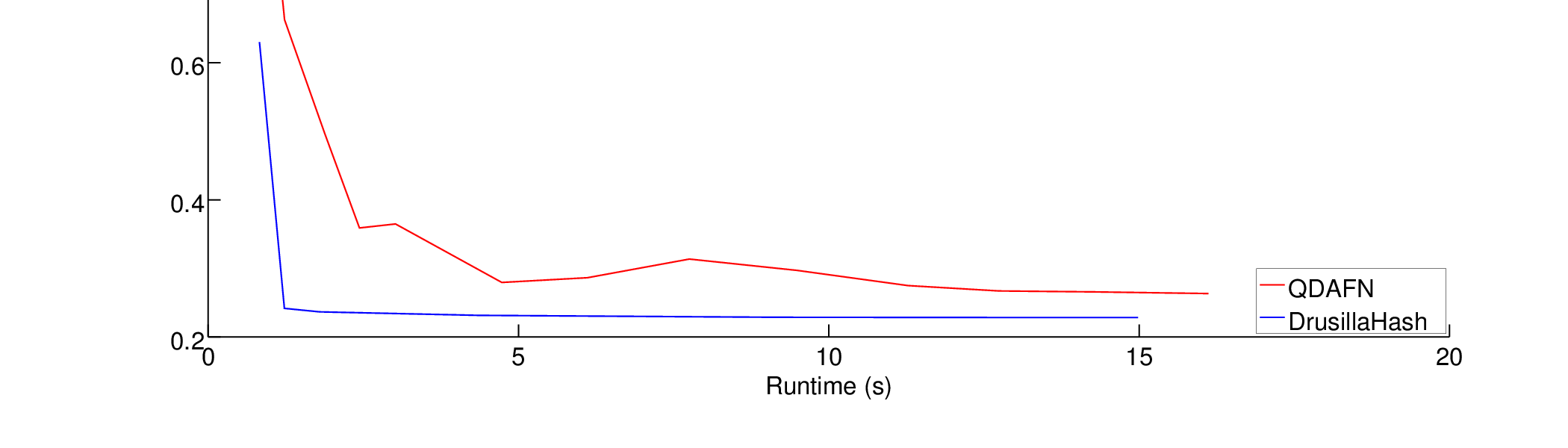
Figure 4: Maximum error for covertype dataset as a function of runtime.

Our experimental results have shown that DrusillaHash gives excellent approximation while only needing to scan few points. Whereas QDAFN seems to perform poorly in high-dimensional settings where the data lie on a low-dimensional manifold (because projection bases are random), DrusillaHash effectively captures the low-dimensional structure with few projection bases.

8 Conclusion

We have proposed an algorithm, DrusillaHash, that builds hash tables for approximate furthest neighbor search using the properties of the dataset to choose the projection bases. This algorithm design is motivated by our empirical analysis of the structure of the approximate furthest neighbor search problem, and the algorithm performs quite compellingly in practice. It scales better with dataset size than other techniques.

We have also proposed a variant, GuaranteedDrusillaHash, which is able to give an absolute approximation guarantee. This is a benefit that no other furthest neighbor hashing scheme is able to provide. However, this variant is not likely to be useful in practice.

Interesting future directions for this line of research may include combining a random projection approach with the approach outlined here. It would also be possible to generalize our approach to arbitrary distance metrics, including those where the points lie in an unrepresentable space. This could be done using techniques similar to some that have been used for max-kernel search [25, 26].

References

- [1] A. Said, B. Kille, B.J. Jain, and S. Albayrak. Increasing diversity through furthest neighbor-based recommendation. Proceedings of the Fifth International Conference on Web Search and Data Mining (WSDM 2012), 12, 2012.
- [2] A. Said, B. Fields, B.J. Jain, and S. Albayrak. User-centric evaluation of a k-furthest neighbor collaborative filtering recommender algorithm. In Proceedings of the 2013 conference on Computer Supported Cooperative Work, pages 1399–1408. ACM, 2013.
- [3] N. Vasiloglou, A.G. Gray, and D.V. Anderson. Scalable semidefinite manifold learning. In Proceedings of the 2008 IEEE Workshop on Machine Learning for Signal Processing, 2008 (MLSP 2008), pages 368–373. IEEE, 2008.
- [4] D. Defays. An efficient algorithm for a complete link method. The Computer Journal, 20(4):364–366, 1977.
- [5] P.D. Schloss, S.L. Westcott, T. Ryabin, J.R. Hall, M. Hartmann, E.B. Hollister, R.A. Lesniewski, B.B. Oakley, D.H. Parks, C.J. Robinson, J.W. Sahl, B. Stres, G.G. Thallinger, D.J. Van Horn, and C.F. Weber. Introducing mothur: open-source, platform-independent, community-supported software for describing and comparing microbial communities. Applied and Environmental Microbiology, 75(23):7537–7541, 2009.
- [6] C.J. Veenman, M.J.T. Reinders, and E. Backer. A maximum variance cluster algorithm. IEEE Transactions on Pattern Analysis and Machine Intelligence, 24(9):1273–1280, 2002.
- [7] O. Cheong, C.-S. Shin, and A. Vigneron. Computing farthest neighbors on a convex polytope. Theoretical Computer Science, 296(1):47–58, 2003.
- [8] R.R. Curtin, W.B. March, P. Ram, D.V. Anderson, A.G. Gray, and C.L. Isbell Jr. Tree-independent dual-tree algorithms. In Proceedings of the 30th International Conference on Machine Learning (ICML ’13), 2013.
- [9] M. Datar, N. Immorlica, P. Indyk, and V.S. Mirrokni. Locality-sensitive hashing scheme based on -stable distributions. In Proceedings of the Twentieth Annual Symposium on Computational Geometry (SoCG ’04), pages 253–262. ACM, 2004.
- [10] P. Indyk and R. Motwani. Approximate nearest neighbors: towards removing the curse of dimensionality. In Proceedings of the Thirtieth Annual ACM Symposium on Theory of Computing (STOC ’98), pages 604–613. ACM, 1998.
- [11] A. Andoni and P. Indyk. Near-optimal hashing algorithms for approximate nearest neighbor in high dimensions. In 47th Annual IEEE Symposium on Foundations of Computer Science (FOCS ’06), pages 459–468. IEEE, 2006.
- [12] R. Pagh, F. Silvestri, J. Sivertsen, and M. Skala. Approximate furthest neighbor in high dimensions. In Similarity Search and Applications, pages 3–14. Springer, 2015.
- [13] P. Indyk. Better algorithms for high-dimensional proximity problems via asymmetric embeddings. In Proceedings of the Fourteenth Annual ACM-SIAM Symposium on Discrete Algorithms (SODA 2003), pages 539–545. Society for Industrial and Applied Mathematics, 2003.
- [14] G.T. Toussaint and B.K. Bhattacharya. On geometric algorithms that use the furthest-point voronoi diagram. School of Computer Science, McGill University, Tech. Rept. No. 81.3, 1981.
- [15] A. Beygelzimer, S. Kakade, and J. Langford. Cover trees for nearest neighbor. In Proceedings of the 23rd International Conference on Machine Learning (ICML ’06), pages 97–104. ACM, 2006.
- [16] R.R. Curtin, D. Lee, W.B. March, and P. Ram. Plug-and-play dual-tree algorithm runtime analysis. Journal of Machine Learning Research, 16:3269–3297, 2015.
- [17] R.R. Curtin. Faster dual-tree traversal for nearest neighbor search. In Similarity Search and Applications, pages 77–89. Springer, 2015.
- [18] S. Bespamyatnikh. Dynamic algorithms for approximate neighbor searching. In Proceedings of the 8th Canadian Conference on Computational Geometry (CCCG’96), pages 252–257, 1996.
- [19] J.L. Bentley. Multidimensional binary search trees used for associative searching. Communications of the ACM, 18(9):509–517, 1975.
- [20] S. Arya, D.M. Mount, N.S. Netanyahu, R. Silverman, and A.Y. Wu. An optimal algorithm for approximate nearest neighbor searching in fixed dimensions. Journal of the ACM (JACM), 45(6):891–923, 1998.
- [21] A. Gionis, P. Indyk, R. Motwani, et al. Similarity search in high dimensions via hashing. In Proceedings of the Twenty-Fifth International Conference on Very Large Data Bases (VLDB ’99), volume 99, pages 518–529, 1999.
- [22] A.G. Gray and A.W. Moore. ‘N-Body’ problems in statistical learning. In Advances in Neural Information Processing Systems 14 (NIPS 2001), volume 4, pages 521–527, 2001.
- [23] M. Lichman. UCI Machine Learning Repository, http://archive.ics.uci.edu/ml, University of California Irvine, School of Information and Computer Sciences, 2013.
- [24] R.R. Curtin, J.R. Cline, N.P. Slagle, W.B. March, P. Ram, N.A. Mehta, and A.G. Gray. mlpack: A scalable C++ machine learning library. The Journal of Machine Learning Research, 14(1):801–805, 2013.
- [25] R.R. Curtin, P. Ram, and A.G. Gray. Fast exact max-kernel search. In Proceedings of the 2013 SIAM International Conference on Data Mining (SDM ’13), pages 1–9. SIAM, 2013.
- [26] R.R. Curtin and P. Ram. Dual-tree fast exact max-kernel search. Statistical Analysis and Data Mining, 7(4):229–253, 2014.