Magnetic Excitations and Electronic Interactions in Sr₂CuTeO₆:
A Spin-1/2 Square Lattice Heisenberg Antiferromagnet

Abstract

Sr₂CuTeO₆ presents an opportunity for exploring low-dimensional magnetism on a square lattice of $S=1/2$ Cu²⁺ ions. We employ ab initio multi-reference configuration interaction calculations to unravel the Cu²⁺ electronic structure and to evaluate exchange interactions in Sr₂CuTeO₆. The latter results are validated by inelastic neutron scattering using linear spin-wave theory and series-expansion corrections for quantum effects to extract true coupling parameters. Using this methodology, which is quite general, we demonstrate that Sr₂CuTeO₆ is an almost ideal realization of a nearest-neighbor Heisenberg antiferromagnet but with relatively weak coupling of 7.18(5) meV.

Mott insulators are a subject of intense interest due to the observation of many different quantum phenomena Khomskii (2014); Witczak-Krempa et al. (2014). In low-dimensional systems, frustration and quantum fluctuations can destroy long-range magnetic order giving rise to quantum paramagnetic phases such as valence-bond solids with broken lattice symmetry or spin liquids, where symmetry is conserved but with possible new collective behaviors involving emergent gauge fields and fractional excitations Anderson (1973, 1987); Balents (2010). The spin-1/2 frustrated square-lattice with nearest-neighbor (NN) $J_{1}$ and next-nearest neighbor $J_{2}$ exchange interactions is one of the simplest models for valence-bond solids and spin liquids Anderson (1987); Shirane et al. (1987). Yet, despite the many theoretical efforts, experimental realizations of the $J_{1}$-$J_{2}$ model have been rather scarce. The double perovskite oxides are particularly interesting as magnetic interactions can be tuned by changing structure, stoichiometry and cation order King and Woodward (2010); Vasala and Karppinen (2015). In the search for a quantum magnet with weak exchange energies, Sr₂CuTeO₆ has been proposed Iwanaga et al. (1999); Koga et al. (2014).

The tetragonal crystal structure of the double perovskite Sr₂CuTeO₆ Reinen and Weitzel (1976) consists of corner sharing CuO₆ and TeO₆ octahedra that are rotated in a staggered fashion about the $c$-axis; see Figs. 1(a) and 1(b). The CuO₆ octahedra are elongated along the $c$-axis, effectively resulting in the ground state of a Cu²⁺ ($3d^{9}$) ion having a hole in the in-plane $d_{x^{2}-y^{2}}$ orbital, where $z$ is along the $c$-axis. This could eventually result in quasi-2D magnetism in Sr₂CuTeO₆  with dominant intra-plane exchange interactions. In the basal $ab$-plane, the exchange that couples the Cu²⁺ ions is the super-superexchange interaction mediated through the bridging TeO₆ octahedra as shown in Fig. 1(b), which is expected to reduce the coupling strength in Sr₂CuTeO₆.

Magnetic susceptibility and heat capacity measurements on Sr₂CuTeO₆  indicate a quasi-2D magnetic behavior, suggesting that it is a realization of the square-lattice $J_{1}$-$J_{2}$ model Koga et al. (2014). More recently, neutron diffraction measurements on Sr₂CuTeO₆ have shown it to order in a Néel antiferromagnetic (AFM) structure below $T_{\rm N}\simeq 29$ K with moments in the $ab$-plane Koga et al. (2016); see Fig. 1(a). The ordered moment at 1.5 K was found to be reduced to 0.69(6) $\mu_{\rm B}$, from the classical value of 1 $\mu_{\rm B}$ Koga et al. (2016), indicating a renormalization by quantum fluctuations Reger and Young (1988); Singh (1989). These observations demand further investigation into the magnetic ground state and excitations that elucidate the role of quantum effects in Sr₂CuTeO₆.

In this Letter, we show that Sr₂CuTeO₆ is an almost ideal realization of a two-dimensional square lattice Heisenberg antiferromagnet. This is achieved by a novel ab initio configuration interaction calculation of relevant exchange interactions, which are reaffirmed by modeling the inelastic magnetic spectrum using spin-wave theory and correcting the exchange interactions by series expansion.

Let us first consider the electronic interactions in Sr₂CuTeO₆. For a Cu²⁺ ($3d^{9}$) ion in O₆ octahedral ligand cage, the degenerate $3d$ levels are split into low-energy $t_{2g}$ and high-energy $e_{g}$ manifolds with a hole in the latter. In the tetragonally elongated CuO₆ octahedra in Sr₂CuTeO₆, the degeneracy of $t_{2g}$ and $e_{g}$ is further reduced into states with $e^{\prime}_{g}$, $b_{2g}$ ($t_{2g}$), and $b_{1g}$, $a_{1g}$ ($e_{g}$) symmetry as shown in Fig 1(c). The ground state wavefunction composition of Cu²⁺ in Sr₂CuTeO₆  and the $d$-level excited state energies and corresponding wavefunctions are summarized in Table 1. These are obtained from calculations at complete-active-space self-consistent-field (CASSCF) and multireference configuration-interaction (MRCI) levels of the many-body wavefunction theory Helgaker et al. (2000),

Table 1: Relative energies of the Cu²⁺ ion $d$-level excitations in Sr₂CuTeO₆(in hole representation). The composition of wavefunctions at the CASSCF level is also provided. Only the five $3d$ orbitals of the Cu²⁺ ion were included in the CASSCF active space. At MRCI level, the wavefunction would also contain contributions from the other correlated orbitals (see text).

Symmetry	Relative E (eV)	CASSCF
of $d^{9}$ states	CASSCF/MRCI	wavefunction
$a_{1g}$	0.00/0.00	$0.97\,|d_{x^{2}-y^{2}}\rangle+0.24\,|d_{xy}\rangle$
$b_{2g}$	0.778/0.856	$-0.24\,|d_{x^{2}-y^{2}}\rangle+0.97\,|d_{xy}\rangle$
$b_{1g}$	0.796/0.863	$1.0\,|d_{z^{2}}\rangle$
$e^{\prime}_{g}$	1.013/1.098	$0.94\,|d_{yz}\rangle-0.34\,|d_{zx}\rangle$
	1.013/1.098	$0.34\,|d_{yz}\rangle+0.94\,|d_{zx}\rangle$

on embedded clusters of atoms containing a single reference CuO₆ octahedron and the surrounding six TeO₆ octahedra; see Supplemental Material for computational details. In contrast to correlated calculations based on density functional theory in conjunction with dynamical mean field theory (DFT+DMFT), our calculations are parameter free and accurately describe correlations within the cluster of atoms in a systematic manner. An active space of nine electrons in five $3d$ orbitals of the Cu²⁺ ion was considered at the CASSCF level to capture the correlations among the $3d$ electrons. In the subsequent correlated calculation, on top of the CASSCF wavefunction all single and double (MR-SDCI) excitations were allowed from the Cu $3s,3p,3d$ and O $2p$ orbitals of the reference CuO₆ octahedron into virtual orbital space to account for correlations involving those electrons Hozoi et al. (2011); Huang et al. (2011). All calculations were done using the molpro quantum chemistry package Werner et al. (2012).

From Table 1 it is evident that, at the CASSCF level, the ground state hole orbital predominantly has $d_{x^{2}-y^{2}}$ character with a small $d_{xy}$ component. This admixture is due to the staggered rotation of CuO₆ and TeO₆ octahedra. Note that the wavefunction obtained in the MR-SDCI calculation also contains non-zero weights from those configurations involving single and double excitations into O $2p$ orbitals. The MR-SDCI calculations predict the lowest crystal field excitation ($a_{1g}$–$b_{1g}$ and $a_{1g}$–$b_{2g}$) to be nearly degenerate at 0.86 eV, an accidental degeneracy very specific to Sr₂CuTeO₆. The highest $d$-level excitation is at 1.01 eV; see Fig. 1(c). It is interesting to note that the on-site $d$-$d$ excitations in Sr₂CuTeO₆  occur at rather low energies in comparison with 1D or 2D layered cuprates Sala et al. (2011); Hozoi et al. (2011); Huang et al. (2011). The presence of highly charged Te⁶⁺ ions around the CuO₆ octahedron effectively decrease the effect of the ligand field on the Cu $d$-orbitals Note (1), a phenomenon observed in layered perovskite compound Sr₂IrO₄ Bogdanov et al. (2015).

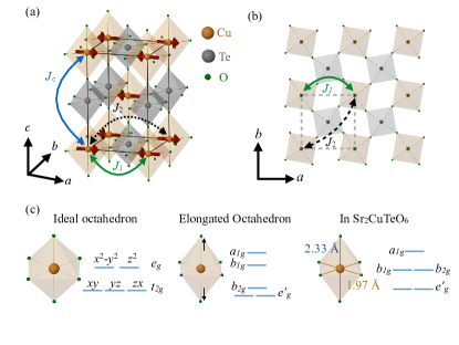
Figure 1: (a) and (b) Crystallographic and magnetic structure of Sr₂CuTeO₆. The Cu²⁺ ions order magnetically into an arrangement indicated by the red arrows. The different exchange couplings are shown by arrows connecting two Cu²⁺ ions. (c) Energy level diagram of $d$-states in octahedral ($O_{h}$) symmetry, for a tetragonally elongated octahedron and for the Cu²⁺ ion in Sr₂CuTeO₆ whose Cu-O bond lengths are labeled.

Having established the ground state hole orbital character and Cu²⁺ on-site $d$-$d$ excitations in Sr₂CuTeO₆ , we evaluate the exchange interactions shown in Fig. 1(a). The exchange couplings were derived from a set of three different MRCI calculations on three different embedded clusters. To estimate $J_{1}$ a cluster consisting of two active CuO₆ octahedral units and two bridging TeO₆ octahedra was considered, for $J_{2}$ and $J_{c}$ only one bridging TeO₆ octahedron was included in the active region Note (1).

The coupling constants were obtained by mapping the energies of the magnetic configurations of the two unpaired electrons in two Cu²⁺ ions onto that of a two-spin Heisenberg Hamiltonian ${\mathcal{H}}_{ij}=J_{ij}\mathbf{S}_{i}\cdot\mathbf{S}_{j}$. A CASSCF reference wavefunction with two electrons in the two Cu²⁺ ground state $d_{x^{2}-y^{2}}$-type orbitals was first constructed for the singlet and triplet spin multiplicities de Graaf and Broer (2015), state averaged. In the MRCI calculations the electrons in the doubly occupied Cu $3d$ orbitals and the Te $4d$ and O $2p$ orbitals of the bridging TeO₆ octahedron were correlated. We adopted a difference dedicated configuration interaction (MR-DDCI) scheme Miralles et al. (1992, 1993) recently implemented within molpro, where a subset of the MR-SDCI determinant space that excludes all the double excitations from the inactive orbitals to the virtuals, is used to construct the many-body wavefunction. This approach has resulted in exchange couplings for several quasi-2D and quasi-1D cuprates that are in excellent agreement with experimental estimates, e.g. see Ref. Muñoz et al., 2000; *cuo2_j_illas_04; *cuo2_dm_pradipto_2012; *j_licu2o2_pradipto_2012.

In Table 2 the Heisenberg couplings derived at the CASSCF and MR-DDCI level with Davidson corrections for size-consistency errors Cave and Davidson (1988) are listed. We see that all the interactions are AFM. At the fully correlated MR-DDCI level of calculation we obtain the in-plane exchange coupling $J_{1}$ to be the largest at 7.39 meV. At the CASSCF level where the Anderson type of exchange is accounted for, i.e, related to intersite $d$-$d$ excitations of the $d_{x^{2}-y^{2}}^{0}$–$d_{x^{2}-y^{2}}^{2}$ type Anderson (1950, 1959), only 30% of the $J_{1}$ exchange is obtained. The MR-DDCI treatment, which now includes excitations of the kind $t_{2g}^{5}e_{g}^{1}$ – $t_{2g}^{6}e_{g}^{2}$, etc., and O $2p$ to Cu 3$d$ charge-transfer virtual states as well, enhances $J_{1}$. Our calculations estimate a second neighbor in-plane coupling $J_{2}=0.007J_{1}$ and the coupling along the $c$-axis to be practically zero; see Table 2.

Although it may perhaps be expected that the dominant superexchange comes from bridging Te $4d$-orbitals – the path Cu²⁺-O^2--Te⁶⁺-O^2--Cu²⁺, we find that the Te outer most occupied $4d$ orbitals are core-like at $\approx 50$ eV below the valence Cu $3d$ and the oxygen $2p$ orbitals, and, hence, a negligible contribution to the magnetic exchange. A MR-DDCI calculation that does not take into account the virtual hopping through the Te $d$ states results in $J_{1}=7.79$ meV. Thus we conclude that the dominant superexchange path is Cu²⁺-O^2--O^2--Cu²⁺ along the two bridging TeO₆ octahedra; see  Note (1). Interestingly, we find that the superexchange involving virtual hoppings from the doubly occupied Cu $3d$ orbitals of $t_{2g}$ symmetry and the $d_{z^{2}}$ of $e_{g}$ symmetry,   0.86-1.1 eV lower than the $d_{x^{2}-y^{2}}$ orbitals (see Table 1), contribute almost half to the exchange coupling – a calculation without the doubly occupied Cu $d$ orbitals in the inactive space result in a $J_{1}$ of 4.51 meV.

Table 2: Heisenberg exchange couplings derived from ab initio CASSCF/MR-DDCI data and experimentally for Sr₂CuTeO₆. The experimental in-plane couplings were obtained from fits to INS using SWT and corrected by SE; see text. Values are given in meV.

$J$	CASSCF	MR-DDCI	Experimental
$J_{1}$	2.320	7.386	7.18(5)
$J_{2}$	0.006	0.051	0.21(6)
$J_{c}$	0.000	0.003	0.04

Next, we turn to inelastic powder neutron scattering (INS) measurements to determine experimentally the nature of magnetic interactions. The experiments were performed at Paul Scherrer Institute, using the spectrometer FOCUS (not shown), and Institut Laue-Langevin on the thermal time-of-flight spectrometer IN4 Cicognani et al. (2000).

The data were collected on a sealed Al envelope containing 24.1 g of Sr₂CuTeO₆ powder at temperatures of 2, 60, and 120 K with incident neutron energy of 25.2 meV and Fermi chopper at 250 Hz. The raw data were corrected for detector efficiency, time-independent background, attenuation, and normalized to a vanadium calibration following standard procedures using LAMP and Mslice software packages LAMP, the Large Array Manipulation Program ; *mslice.

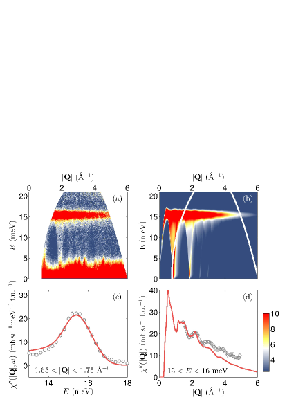
Figure 2: (a) Dynamic susceptibility $\chi^{\prime\prime}(|\mathbf{Q}|,E)$ map obtained by subtraction of 120 K from 2 K data. (b) Calculated powder average inelastic spectrum using $\tilde{J}_{1}=7.60(3)$ and $\tilde{J}_{2}=0.60(3)$ meV. The solid white lines show the detector edges. The SWT intensity is scaled to match the measured pattern in units of mb sr^-1 meV^-1f.u.^-1. (c) A constant wavevector cut for $|\mathbf{Q}|\approx 1.7$ Å^-1 through the dynamic susceptibility with a solid red line showing the calculated cut from SWT. (d) $|\mathbf{Q}|$-dependence of the magnetic band around 15.4 meV and a comparison to SWT calculations.

The spin-spin correlations between Cu ions can be probed using INS as a function of momentum and energy transfer $(|\mathbf{Q}|,\hbar\omega)$, where the former is defined as $|\mathbf{Q}|=|h\mathbf{a}^{\ast}+k\mathbf{b}^{\ast}+l\mathbf{c}^{\ast}|$ in terms of reciprocal lattice vectors. The magnetic neutron scattering cross-section is directly related to the imaginary part of the dynamical susceptibility $\chi^{\prime\prime}(|\mathbf{Q}|,\omega)$. At sufficiently high temperatures above $T_{\rm N}$, the magnetic excitations are generally heavily damped and uncorrelated Rønnow et al. (2001). In the case of Sr₂CuTeO₆, some magnetic correlations persist even at 60 K ($\approx 2T_{\rm N}$), indicative of the low-dimensionality of the system, see Ref. Note (1). On warming to 120 K, the magnetic signal can no longer be observed and we subtract this data from the 2 K measurements to reveal a purely magnetic contribution to the signal.

In Fig. 2 we present the measured and calculated magnetic spectra. Figure 2(a) shows the inelastic powder $\chi^{\prime\prime}(|\mathbf{Q}|,\omega)$ spectrum mapped over momentum and energy transfer. We observe dispersive modes originating from the magnetic Bragg peak positions around $|\mathbf{Q}|=0.9$ and 1.87 Å^-1, which correspond to $(0.5,0.5,0)$ and $(1.5,0.5,0)$. The dispersion is linear, which is consistent with AFM spin waves and remains gapless within the energy resolution of our measurements of 1.4 meV at the elastic line (FWHM).

The dominant feature in our spectrum is a strong, flat band around 15.4 meV, shown in Fig. 2(c). The intensity decreases with increasing $|\mathbf{Q}|$ as expected for magnetic scattering; see Fig. 2(d). For low-dimensional systems, powder averaging produces a van Hove-like maximum at the zone boundary. Therefore, we interpret the flat band as due to the zone boundaries and not to a dispersionless excitation. We observe that the signal at 15.4 meV has a FWHM of 1.7 meV, which is significantly larger than the 1.2 meV instrumental resolution at this energy transfer. This implies that there is dispersion along the zone boundary.

There are two potential sources of zone boundary dispersion. First, a finite $J_{2}$ leads to dispersion along the zone boundary. This effect can be captured by spin wave theory (SWT). Second, it has been well established that even the purely nearest neighbor ($J_{2}=0$) spin-$1/2$ Heisenberg antiferromagnet on a square lattice exhibits a quantum effect with two results: (i) at $(\pi,0)$ the sharp spin-wave peak develops a lineshape extending towards higher energies – a quantum effect that has often been explained in terms of spinon deconfinement Dalla Piazza et al. (2015); ii) a 6%-8% zone boundary dispersion where $E(\pi,0)$ is lower than $E(\pi/2,\pi/2)$. The latter effect cannot be captured by SWT but by several other theoretical approaches – series expansion (SE) Singh and Gelfand (1995); Zheng et al. (2005), exact diagonalization Chen et al. (1992), quantum Monte-Carlo (QMC) Syljuåsen and Rønnow (2000); Sandvik and Singh (2001), variational wave-function (VA) Dalla Piazza et al. (2015), etc. In the presence of an AFM $J_{2}$ coupling, the quantum dispersion and the $J_{2}$ dispersion reenforce each other.

For calculating the powder-averaged neutron spectra, the classical (large-$S$) linear spin-wave (SWT) works best, owing to significantly faster computation time. Therefore, our approach is to fit the magnetic spectrum using SWT to extract effective $\tilde{J}_{1}$ and $\tilde{J}_{2}$ parameters and then to use SE to correct these values to obtain true $J_{1}$ and $J_{2}$ parameters. In doing so, we consider a Heisenberg Hamiltonian, $\mathcal{H}=\tilde{J}_{1}\sum_{\langle ij\rangle}\mathbf{S}_{i}\cdot\mathbf{S}_{j}+\tilde{J}_{2}\sum_{\langle ij\rangle}\mathbf{S}_{i}\cdot\mathbf{S}_{j}$. We neglect the very small $c$-axis coupling as obtained in our calculations, see Table 2. The magnetic dispersion can be described as $\hbar\omega=Z_{c}\sqrt{A^{2}-B^{2}}$, where $A=2\tilde{J}_{1}+\tilde{J}_{2}[\cos(2\pi h-2\pi k)+\cos(2\pi h+2\pi k)-2]$ and $B=\tilde{J}_{1}(\cos 2\pi h+\cos 2\pi k)$ . To fit the data we calculate the imaginary part of the dynamic susceptibility including an anisotropic Cu²⁺ magnetic form factor Brown (2006); Zhu (2005). The resulting spectrum is shown in Fig. 2(b) which has been calculated using $\tilde{J}_{1}=7.60(3)$ and $\tilde{J}_{2}=0.60(3)$ meV. Comparing the spectra in Figs. 2(a) and 2(b), we find good agreement across the entire wavevector and energy transfer range. The SWT simulation is able to reproduce the strong flat mode around 15.4 meV and spin-waves emerging from the AFM positions. At larger $|\mathbf{Q}|$, we find that the intensity is predicted to decrease more rapidly than observed; see Fig. 2(d). This could be an artifact of imperfect subtraction of the phonon spectrum, a small mixing of the $d_{xy}$ orbitals influencing the magnetic form factor or multiple scattering.

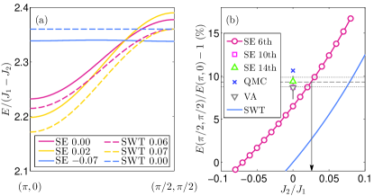
Figure 3: (a) Dispersion between $(\pi,0)$ and $(\pi/2,\pi/2)$ calculated using SE and SWT methods for $J_{1}=1$ and $J_{2}/J_{1}$ values given in the legend. (b) Calculated change of zone boundary energies at $(\pi,0)$ and $(\pi/2,\pi/2)$ obtained from SE and SWT. The dashed horizontal line denotes the dispersion expected for the calculated ratio of $\tilde{J}_{2}/\tilde{J}_{1}=0.078$ and the horizontal lines either side show the corresponding uncertainty of $\pm 0.005$ in $\tilde{J}_{2}/\tilde{J}_{1}$.

We now turn to the series-expansion method up to 6th order for $J_{1}$-$J_{2}$ to correct the exchange coupling parameters derived from SWT for the quantum effects Singh and Gelfand (1995); Tsyrulin et al. (2009). Figure 3(a) shows the calculated single-magnon energies for the SE and SWT calculations for different relative strengths $J_{2}/J_{1}$ and $\tilde{J}_{2}/\tilde{J}_{1}$. We employ the convention where $(\pi/2,\pi/2)$ and $(\pi,0)$ correspond to points $(h,k)=(1/2,0)$ and $(1/4,1/4)$ (and equivalent) in reciprocal space, respectively. The SE calculations show a zone-boundary dispersion of around 7% when second neighbor exchange is absent. Comparing this to SWT calculations, see Fig. 3(a), it is clear that a non-zero AFM $\tilde{J}_{2}$ parameter modifies this part of the dispersion in a similar manner.

From SWT fits, we find that $\tilde{J}_{2}/\tilde{J}_{1}=0.079(3)$ which leads to a 9.3(5)% dispersion between $(\pi/2,\pi/2)$ and $(\pi,0)$. However, in SE, the same dispersion is explained largely by quantum fluctuations, see Fig. 3(b), such that $J_{2}/J_{1}=0.025(5)$, or $J_{2}=0.21(6)$ meV. By correcting the SWT results by SE, we obtain a more realistic value of the ratio of the exchange coupling parameters. The zone boundary dispersion can be estimated by other theoretical approaches for $J_{2}=0$ Dalla Piazza et al. (2015); Chen et al. (1992); Syljuåsen and Rønnow (2000); Sandvik and Singh (2001); Zheng et al. (2005). In Fig. 3(a) we show that the same amount of dispersion as we observe can also be explained in the absence of $J_{2}$ interaction. Nonetheless, our experimental results place an upper limit on the size of $J_{2}$. We note that reducing $J_{2}$ must increase $J_{1}$ accordingly $J_{1}\approx\tilde{J}_{1}(1-\tilde{J}_{2}/\tilde{J}_{1})/(1-J_{2}/J_{1})$, which results in $J_{1}\approx 7.18(5)$ meV. For a quasi-2D system, $T_{\rm N}$ can be used to estimate the coupling $J_{c}$ between layers using $T_{\rm N}\approx J_{c}[\xi(T_{\rm N})/a]^{2}$. We find the correlation length is $\xi(T_{\rm N})/a\approx 10$ from three-loop order given in Ref. Hasenfratz and Niedermayer (1991). This gives an out-of-plane coupling on the order of 0.04 meV. Comparing experimentally obtained exchange parameters with ab initio calculations in Table 2, we find remarkably good agreement. Indeed, this demonstrates the power of our approach in obtaining a complete description of the magnetic interactions which has rather rarely been applied to strongly correlated electron systems.

We note that neutron scattering measurements have recently been performed on the related Sr₂CuWO₆ compound where the $J_{2}\gg J_{1}$ leads to columnar antiferromagnetic order Walker et al. (2016); Burrows et al. . Exchange parameters have been estimated using calculations based on density functional theory corrected for Hubbard type interactions and are in reasonable agreement with experiments without corrections for quantum fluctuations Walker et al. (2016); Burrows et al. . It would be interesting to validate the proposed exchange interaction mechanisms in Sr₂CuWO₆ using more accurate many-body calculations similar to those adopted in this work.

In summary, we have characterized magnetic interactions in a new layered antiferromagnet Sr₂CuTeO₆ using detailed ab initio configuration interaction calculations and inelastic neutron scattering measurements. The calculations accurately predict the exchange interactions, and further determine the dominant exchange path i.e via Cu²⁺-O^2--O^2--Cu²⁺ and not via Te 4$d$ orbitals, as previously suggested. By simulating the magnetic excitations using classical SWT corrected by SE, we show that NN exchange coupling is around 7.18(5) meV with very weak next-nearest interactions on the order of $<3$% of $J_{1}$. The low-energy scale of interactions in Sr₂CuTeO₆ should make it an appealing system to study theoretically and experimentally as an almost ideal realization of a nearest-neighbor Heisenberg antiferromagnet. Moreover, our work brings to the fore a novel strategy for exploring Heisenberg antiferromagnets from ab initio calculations to simulations of magnetic spectra taking into account quantum effects.

Appendix A Supplemental Material

Appendix B Multi-reference configuration interaction calculations

B.1 Ground state of Cu²⁺ ion and $d$-level excitations

A cluster consisting of a single CuO₆ octahedron surrounded with six TeO₆ octahedra and the eight Sr ions was considered for calculating the Cu²⁺ ground state and on-site $d-d$ excitations. The surrounding solid-state matrix was modeled as a finite array of point charges fitted to reproduce the crystal Madelung field in the cluster region Klintenberg et al. (2000). We employed all electron atomic natural orbital (ANO) basis sets of quadruple-zeta quality for the central Cu²⁺ ion Pou-Amerigo et al. (1995) and triple-zeta functions for the oxygens Widmark et al. (1990) of the central CuO₆ unit. Additionally three polarization $f$-functions for the Cu ion and two $d$-functions for the oxygens were used. The Te ions were represented by energy-consistent pseudopotentials and triple-zeta basis sets for the valence shells Bergner et al. (1993) and oxygens connected to the Te ions were represented with ANO [$2s1p$] functions K. Pierloot and Roos (1995). For the Sr²⁺ ions we used total-ion effective potentials and a single $s$ valence basis function Fuentealba et al. (1985).

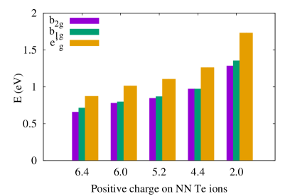
Figure 4: (Color online) Excited state energies of $d$-manifold of the Cu²⁺ ion for varying charges on the NN Te ions.

As mentioned in the main text, the on-site $d$-$d$ excitations in Sr₂CuTeO₆ occur at rather low energies in comparison with other cuprate compounds. To verify that this is due to the highly charged Te⁶⁺ ions surrounding the CuO₆ octahedron, we calculated the $d$-level energies for several scenarios with different charges on the neighboring Te ions. As shown in Fig. 4, as the charge on the NN Te ions decreases, the $d-d$ excitation energies increase. For 2+ charge on the NN Te ions, the excitation energies are very similar to other perovskite cuprates, e.g. La₂CuO₄ Hozoi et al. (2011).

B.2 Magnetic couplings between two Cu²⁺ ions.

Three different clusters were adopted to evaluate $J_{1}$, $J_{2}$ and $J_{c}$, see Fig. 1 in the main text. For $J_{1}$ the cluster consists of two CuO₆ and two TeO₆ octahedra constituting the reference unit and eight surrounding TeO₆ octahedra (buffer region) to describe the charge distribution in the reference region accurately. The cluster for $J_{2}$ consists of a reference unit with two CuO₆ and one bridging TeO₆ octahedra, and the buffer region has ten TeO₆ octahedra and four Cu²⁺ ions surrounding the bridging TeO₆ octahedron. These Cu²⁺ ions were described by closed shell total ion potentials to avoid spin-couplings with the Cu²⁺ ions in the reference region. Such procedure is often used in quantum chemistry calculations for solids, see Ref. Broer et al., 2003; Maurice et al., 2012b; Katukuri et al., 2012. The cluster used for calculating $J_{3}$ is similar to that of the one used for $J_{2}$ calculation. All the Sr²⁺ ions surrounding the reference unit are also considered in all the three clusters. As for the single site calculations, the solid-state matrix was modeled as a finite array of point charges fitted to reproduce the crystal Madelung field in the cluster region.

ANO quadruple-zeta quality basis sets with three polarization $f$-functions were used for the Cu²⁺ ions Pou-Amerigo et al. (1995) of the reference unit and the bridging oxygens were described with quintuple-zeta basis sets and four polarization $d$-functions Widmark et al. (1990). Triple-zeta quality basis functions Widmark et al. (1990) were used for the rest of the O^2- ions in the reference unit. The 28 core electrons of bridging Te ions were represented with effective core potential and the occupied 4$s$, 4$p$, 4$d$ and unoccupied 5$s$, 5$p$ manifolds were represented with [$6s5p4d$] basis functions with two additional polarization $f$-functions Peterson et al. (2003). All the 48 electrons of the Te⁶⁺ ions in the buffer region were modelled with effective core potential and valence 5$s$ and 5$p$ are described with triple-zeta quality basis sets Bergner et al. (1993). For the oxygen ions in the buffer region we used ANO type two $s$ and one $p$ function K. Pierloot and Roos (1995).

To evaluate the accuracy of our embedding scheme, we have calculated the Ising-like coupling, $J_{1}^{I}$, for the Cu-Cu link corresponding to $J_{1}$ using periodic unrestricted Hartree-Fock (UHF) calculations. crystal Dovesi et al. (2014) program package was employed for these periodic UHF calculations. We used triple zeta basis sets for Cu and oxygen from crystal library. Te and Sr ions were treated with effective core potentials with [2s2p] basis functions for the valence electrons Bergner et al. (1993); Fuentealba et al. (1985).

Table 3 summarizes the results of such calculations. The $J_{1}^{I}$ calculated from periodic calculation should be exactly the same as that obtained from our cluster calculation at UHF level of calculation and with the same basis sets if the embedding was exact representation of the solid environment. One can see that there is a difference of 0.8 meV between the periodic and embedded cluster calculations.

Table 3: Ising coupling, $J_{1}^{I}$, calculated using unrestricted Hartree-Fock method with perioding and embedded cluster approaches.

UHF	Relative energies (meV)
	Periodic	Emb. cluster
$J_{1}^{I}$	-0.56	0.25

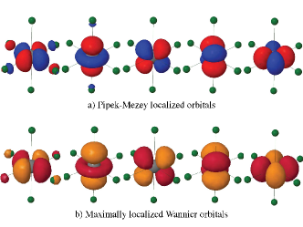
Figure 5: (Color online) Localized Cu $3d$ orbitals, labels from left to right: $d_{x^{2}-y^{2}}$, $d_{z^{2}}$, $d_{xz}$, $d_{yz}$ and $d_{xy}$. a) Orbitals used in our calculations. b) Maximally localized Wannier functions obtained from periodic density functional theory calculations using VASPKresse and Furthmüller (1996) package. Jmol jmo plotting package was used to plots the orbitals.

In the correlated calculations, multiconfiguration reference wave functions were first generated by CASSCF calculations. For two NN CuO₆ octahedra, the finite set of Slater determinants was defined in the CASSCF treatment in terms of two electrons and two Cu $d_{x^{2}-y^{2}}$ type of orbitals. The SCF optimization was carried out for an average of the singlet and triplet states associated with this manifold. On top of the CASSCF reference, the MR-DDCI expansion additionally includes single and double excitations into the virtual orbitals from the reference CAS space and single excitations from the Cu $d$ orbitals not included in the CAS space and the 2$p$ orbitals of the bridging ligands. A similar strategy of explicitly dealing only with selected groups of ligand orbitals was earlier adopted in quantum chemistry studies on both 3$d$ Fink et al. (1994); Calzado et al. (2003); van Oosten et al. (1996) and 5$d$ Katukuri et al. (2014a); Bogdanov et al. (2012); Katukuri et al. (2012, 2014b) compounds, with results in good agreement with the experiment. To separate the Cu 3$d$ and O 2$p$ valence orbitals into different groups, we used the Pipek-Mezey Pipek and Mezey (1989) orbital localization module available in molpro Werner et al. (2012).

In Fig. 5 the Cu $3d$ orbitals obtained by Pipek-Mezey localization and the Cu 3$d$ maximally localized Wannier functions obtained from a periodic density functional theory calculation are shown. The latter were obtained from calculations performed using VASP Kresse and Furthmüller (1996) package with PAW pseudopotentials Kresse and Joubert (1999) and the Wannier90 Mostofi et al. (2014) code. One can see that the ones used in the cluster calculations are very similar to the maximally localized Wannier functions.

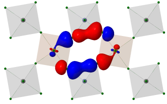
Figure 6: (Color online) The sigma overlapping bridging oxygen 2$p$ orbitals that contribute primarily to the exchange coupling $J_{1}$. The Cu, O and Te atoms are shown in brown, green and grey colors respectively. Jmol jmo plotting package was used to produce the molecular orbitals.

As mentioned in the main text, we find that the super-superexchange path Cu²⁺-O^2--O^2--Cu²⁺ along the two bridging TeO₆ octahedra contributes to the exchange interaction $J_{1}$. In Fig. 6 the bridging O $2p$ orbitals that primarily contribute to the exchange coupling are shown. Table 4 lists the exchange coupling $J_{1}$ obtained when particular O $2p$ orbitals are correlated. The $p_{x}$ type of orbitals have a sigma-type overlap with the Cu $d_{x^{2}-y^{2}}$ orbitals where as the $p_{y}$ are nearly orthogonal and the $p_{z}$ are orthogonal. It can be clearly seen that the sigma overlapping orbitals contribute to the exchange significantly.

Table 4: Exchange coupling $J_{1}$ obtained when selected oxygen bridging $2p$ orbitals are correlated, see text. The values are in meV.

	Correlated orbitals
CASSCF	$p_{x}$	$p_{y}$	$p_{z}$
2.32	6.64	3.71	3.53

Appendix C Magnetic susceptibility

Magnetization measurements were performed using a Quantum Design SQUID magnetometer over a temperature range of 2-800 K using an applied magnetic field of 1000 Oe. This was done in two separate measurements for low-temperature (2-340 K) and high-temperature (300-800 K) regimes. In the latter case, the powder sample was sealed inside an evacuated quartz tube.

In Fig. 7 we show our magnetization measurements as a function of temperature performed on a Sr₂CuTeO₆ sample. We observe a broad peak around 74 K which is characteristic of low-dimensional Heisenberg antiferromagnets and is consistent with previous reports Iwanaga et al. (1999); Koga et al. (2014). Previous estimates of the exchange parameters were based on modelling magnetic susceptibility measurements using quantum Monte Carlo simulations with $J_{1}=6.4$ meV Koga et al. (2014).

Using thermodynamic perturbation expansions for the $J_{1}$-$J_{2}$ system, it is possible to calculate the high-temperature expansion (HTE) of the magnetic susceptibility. Using the exchange parameters obtained from fitting inelastic neutron measurements by spin-wave theory with a correction for quantum effects using series-expansion, we have performed such a calculation using algorithms developed in Ref. Schmidt et al. (2011). Figure 7 shows that the HTE susceptibility obtained using [4,4] Padé approximant describes our data very well across a wide range of temperatures. Furthermore, we can estimate the Weiss temperature in the mean-field approximation from $\theta=-S(S+1)/(3k_{\rm B})\sum z_{i}J_{i}$ to be $-$83.6(6) K, which agrees reasonably well with the independently reported value of $-$97 K for Sr₂CuTeO₆ Iwanaga et al. (1999).

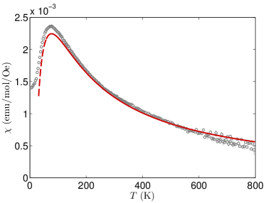
Figure 7: (Color online) (a) Magnetization measurements of Sr₂CuTeO₆ in a 1000 Oe applied field. The red line shows HTE calculations for $J_{1}=7.18$ meV, $J_{2}=0.025$ meV, and $g$-factor of 2.3. Dashed line indicates a 10% difference between the Pade approximation and 8th order series expansion.

Appendix D Temperature dependence of excitations

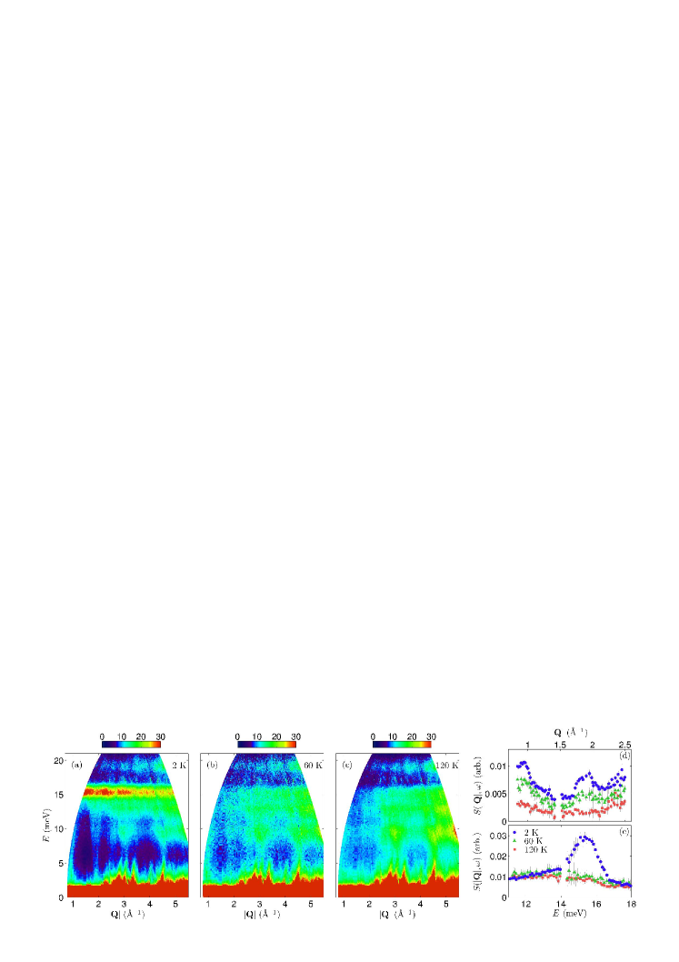
Figure 8: (Color online) Inelastic powder spectra of $S(|\mathbf{Q}|,\omega)$ maps collected at 2, 60 and 120 K (a–c). Representative cuts at constant energy and wavevector are shown in panels (d) $E=5$ meV and (e) $|\mathbf{Q}|=1.7$ Å^-1, respectively. In panel (d), we have displaced the data vertically for clearer presentation.

In the main article we have shown our analysis of the $\chi^{\prime\prime}(|\mathbf{Q}|,\omega)$ which has been calculated through a subtraction of 120 K measurements from 2 K data. In Fig. 8 we instead show the $S(|\mathbf{Q}|,\omega)$ measurements at 2, 60 and 120 K. The base temperature measurements in Fig. 8(a) show that scattering from the phonons is noticeable at larger $|\mathbf{Q}|$. A flat band is observed around 19 meV which we ascribe to be originating from the lattice as its intensity increases with $|\mathbf{Q}|$. At 60 K, see Fig. 8(b), we observe that the intensity of the strong magnetic scattering band at 15.4 meV is greatly suppressed. However, we still find steeply rising excitations around 1 and 1.8 meV emanating from the magnetic Bragg positions. In Fig. 7(d) we plot cuts through this dispersion at 5 meV. This temperature corresponds to approximately 2$T_{\rm N}$. In Fig. 8(c), we observe that phonon scattering has increased and is more prominent at larger $|\mathbf{Q}|$. The magnetic fluctuations are largely gone (smeared out), which is also evident from the $|\mathbf{Q}|$- and energy-cuts in Figs. 8(d) and 8(e). The observation of magnetic fluctuations well above $T_{\rm N}$ which is characteristic of low-dimensional magnets, such as for example CFTD Rønnow et al. (2001). With increasing temperature, we still have magnetic scattering but these become increasingly uncorrelated and by the sum-rule are smeared out over all reciprocal space.