Dynamic index and LZ factorization in compressed space

Abstract

In this paper, we propose a new dynamic compressed index of $O(w)$ space for a dynamic text $T$, where $w=O(\min(z\log N\log^{*}M,N))$ is the size of the signature encoding of $T$, $z$ is the size of the Lempel-Ziv77 (LZ77) factorization of $T$, $N$ is the length of $T$, and $M\geq 4N$ is an integer that can be handled in constant time under word RAM model. Our index supports searching for a pattern $P$ in $T$ in $O(|P|f_{\mathcal{A}}+\log w\log|P|\log^{*}M(\log N+\log|P|\log^{*}M)+\mathit{occ}\log N)$ time and insertion/deletion of a substring of length $y$ in $O((y+\log N\log^{*}M)\log w\log N\log^{*}M)$ time, where $f_{\mathcal{A}}=O(\min\{\frac{\log\log M\log\log w}{\log\log\log M},\sqrt{\frac{\log w}{\log\log w}}\})$. Also, we propose a new space-efficient LZ77 factorization algorithm for a given text of length $N$, which runs in $O(Nf_{\mathcal{A}}+z\log w\log^{3}N(\log^{*}N)^{2})$ time with $O(w)$ working space.

1 Introduction

1.1 Dynamic compressed index

Given a text $T$, the string indexing problem is to construct a data structure, called an index, so that querying occurrences of a given pattern in $T$ can be answered efficiently. As the size of data is growing rapidly in the last decade, many recent studies have focused on indexes working in compressed text space (see e.g. [11, 12, 7, 6]). However most of them are static, i.e., they have to be reconstructed from scratch when the text is modified, which makes difficult to apply them to a dynamic text. Hence, in this paper, we consider the dynamic compressed text indexing problem of maintaining a compressed index for a text string that can be modified. Although there exists several dynamic non-compressed text indexes (see e.g. [24, 3, 9] for recent work), there has been little work for the compressed variants. Hon et al. [15] proposed the first dynamic compressed index of $O(\frac{1}{\epsilon}(NH_{0}+N))$ bits of space which supports searching of $P$ in $O(|P|\log^{2}N(\log^{\epsilon}N+\log|\Sigma|)+\mathit{occ}\log^{1+\epsilon}N)$ time and insertion/deletion of a substring of length $y$ in $O((y+\sqrt{N})\log^{2+\epsilon}N)$ amortized time, where $0<\epsilon\leq 1$ and $H_{0}\leq\log|\Sigma|$ denotes the zeroth order empirical entropy of the text of length $N$ [15]. Salson et al. [26] also proposed a dynamic compressed index, called dynamic FM-Index. Although their approach works well in practice, updates require $O(N\log N)$ time in the worst case. To our knowledge, these are the only existing dynamic compressed indexes to date.

In this paper, we propose a new dynamic compressed index, as follows:

Theorem 1.

Let $M$ be the maximum length of the dynamic text to index, $N$ the length of the current text $T$, $w=O(\min(z\log N\log^{*}M,N))$ the size of the signature encoding of $T$, and $z$ the number of factors in the Lempel-Ziv 77 factorization of $T$ without self-references. Then, there exists a dynamic index of $O(w)$ space which supports searching of a pattern $P$ in $O(|P|f_{\mathcal{A}}+\log w\log|P|\log^{*}M(\log N+\log|P|\log^{*}M)+\mathit{occ}\log N)$ time, where $f_{\mathcal{A}}=O(\min\{\frac{\log\log M\log\log w}{\log\log\log M},\sqrt{\frac{\log w}{\log\log w}}\})$, and insertion/deletion of a (sub)string $Y$ into/from an arbitrary position of $T$ in amortized $O((|Y|+\log N\log^{*}M)\log w\log N\log^{*}M)$ time. Moreover, if $Y$ is given as a substring of $T$, we can support insertion in amortized $O(\log w(\log N\log^{*}M)^{2})$ time.

Since $z\geq\log N$, $\log w=\max\{\log z,\log(\log^{*}M)\}$. Hence, our index is able to find pattern occurrences faster than the index of Hon et al. when the $|P|$ term is dominating in the pattern search times. Also, our index allows faster substring insertion/deletion on the text when the $\sqrt{N}$ term is dominating.

1.1.1 Related work.

To achieve the above result, technically speaking, we use the signature encoding $\mathcal{G}$ of $T$, which is based on the locally consistent parsing technique. The signature encoding was proposed by Mehlhorn et al. for equality testing on a dynamic set of strings [17]. Since then, the signature encoding and the related ideas have been used in many applications. In particular, Alstrup et al.’s proposed dynamic index (not compressed) which is based on the signature encoding of strings, while improving the update time of signature encodings [3] and the locally consistent parsing algorithm (details can be found in the technical report [2]).

Our data structure uses Alstrup et al.’s fast string concatenation/split algorithms (update algorithm) and linear-time computation of locally consistent parsing, but has little else in common than those. Especially, Alstrup et al.’s dynamic pattern matching algorithm [3, 2] requires to maintain specific locations called anchors over the parse trees of the signature encodings, but our index does not use anchors. Our index has close relationship to the ESP-indices [27, 28], but there are two significant differences between ours and ESP-indices: The first difference is that the ESP-index [27] is static and its online variant [28] allows only for appending new characters to the end of the text, while our index is fully dynamic allowing for insertion and deletion of arbitrary substrings at arbitrary positions. The second difference is that the pattern search time of the ESP-index is proportional to the number $\mathit{occ}_{c}$ of occurrences of the so-called “core” of a query pattern $P$, which corresponds to a maximal subtree of the ESP derivation tree of a query pattern $P$. If $\mathit{occ}$ is the number of occurrences of $P$ in the text, then it always holds that $\mathit{occ}_{c}\geq\mathit{occ}$, and in general $\mathit{occ}_{c}$ cannot be upper bounded by any function of $\mathit{occ}$. In contrast, as can be seen in Theorem 1, the pattern search time of our index is proportional to the number $\mathit{occ}$ of occurrences of a query pattern $P$. This became possible due to our discovery of a new property of the signature encoding [2] (stated in Lemma 16).

As another application of signature encodings, Nishimoto et al. showed that signature encodings for a dynamic string $T$ can support Longest Common Extension (LCE) queries on $T$ efficiently in compressed space [20] (Lemma 10). They also showed signature encodings can be updated in compressed space (Lemma 12). Our algorithm uses properties of signature encodings shown in [20], more precisely, Lemmas 5-10 and 12, but Lemma 16 is a new property of signature encodings not described in [20].

In relation to our problem, there exists the library management problem of maintaining a text collection (a set of text strings) allowing for insertion/deletion of texts (see [18] for recent work). While in our problem a single text is edited by insertion/deletion of substrings, in the library management problem a text can be inserted to or deleted from the collection. Hence, algorithms for the library management problem cannot be directly applied to our problem.

1.2 Computing LZ77 factorization in compressed space.

As an application of our dynamic compressed index, we present a new LZ77 factorization algorithm working in compressed space.

The Lempel-Ziv77 (LZ77) factorization is defined as follows.

Definition 2 (Lempel-Ziv77 factorization [29]).

The Lempel-Ziv77 (LZ77) factorization of a string $s$ without self-references is a sequence $f_{1},\ldots,f_{z}$ of non-empty substrings of $s$ such that $s=f_{1}\cdots f_{z}$, $f_{1}=s[1]$, and for $1<i\leq z$, if the character $s[|f_{1}..f_{i-1}|+1]$ does not occur in $s[|f_{1}..f_{i-1}|]$, then $f_{i}=s[|f_{1}..f_{i-1}|+1]$, otherwise $f_{i}$ is the longest prefix of $f_{i}\cdots f_{z}$ which occurs in $f_{1}\cdots f_{i-1}$. The size of the LZ77 factorization $f_{1},\ldots,f_{z}$ of string $s$ is the number $z$ of factors in the factorization.

Although the primary use of LZ77 factorization is data compression, it has been shown that it is a powerful tool for many string processing problems [13, 12]. Hence the importance of algorithms to compute LZ77 factorization is growing. Particularly, in order to apply algorithms to large scale data, reducing the working space is an important matter. In this paper, we focus on LZ77 factorization algorithms working in compressed space.

The following is our main result.

Theorem 3.

Given the signature encoding $\mathcal{G}$ of size $w$ for a string $T$ of length $N$, we can compute the LZ77 factorization of $T$ in $O(z\log w\log^{3}N(\log^{*}M)^{2})$ time and $O(w)$ working space where $z$ is the size of the LZ77 factorization of $T$.

In [20], it was shown that the signature encoding $\mathcal{G}$ can be constructed efficiently from various types of inputs, in particular, in $O(Nf_{\mathcal{A}})$ time and $O(w)$ working space from uncompressed string $T$. Therefore we can compute LZ77 factorization of a given $T$ of length $N$ in $O(Nf_{\mathcal{A}}+z\log w\log^{3}N(\log^{*}M)^{2})$ time and $O(w)$ working space.

1.2.1 Related work.

Goto et al. [14] showed how, given the grammar-like representation for string $T$ generated by the LCA algorithm [25], to compute the LZ77 factorization of $T$ in $O(z\log^{2}m\log^{3}N+m\log m\log^{3}N)$ time and $O(m\log^{2}m)$ space, where $m$ is the size of the given representation. Sakamoto et al. [25] claimed that $m=O(z\log N\log^{*}N)$, however, it seems that in this bound they do not consider the production rules to represent maximal runs of non-terminals in the derivation tree. The bound we were able to obtain with the best of our knowledge and understanding is $m=O(z\log^{2}N\log^{*}N)$, and hence our algorithm seems to use less space than the algorithm of Goto et al. [14]. Recently, Fischer et al. [10] showed a Monte-Carlo randomized algorithms to compute an approximation of the LZ77 factorization with at most $2z$ factors in $O(N\log N)$ time, and another approximation with at most $(i+\epsilon)z$ factors in $O(N\log^{2}N)$ time for any constant $\epsilon>0$, using $O(z)$ space each.

Another line of research is LZ77 factorization working in compressed space in terms of Burrows-Wheeler transform (BWT) based methods. Policriti and Prezza recently proposed algorithms running in $NH_{0}+o(N\log|\Sigma|)+O(|\Sigma|\log N)$ bits of space and $O(N\log N)$ time [21], or $O(R\log N)$ bits of space and $O(N\log R)$ time [22], where $R$ is the number of runs in the BWT of the reversed string of $T$. Because their and our algorithms are established on different measures of compression, they cannot be easily compared. For example, our algorithm is more space efficient than the algorithm in [22] when $w=o(R)$, but it is not clear when it happens.

2 Preliminaries

2.1 Strings

Let $\Sigma$ be an ordered alphabet. An element of $\Sigma^{*}$ is called a string. For string $w=xyz$, $x$, $y$ and $z$ are called a prefix, substring, and suffix of $w$, respectively. The length of string $w$ is denoted by $|w|$. The empty string $\varepsilon$ is a string of length $0$. Let $\Sigma^{+}=\Sigma^{*}-\{\varepsilon\}$. For any $1\leq i\leq|w|$, $w[i]$ denotes the $i$-th character of $w$. For any $1\leq i\leq j\leq|w|$, $w[i..j]$ denotes the substring of $w$ that begins at position $i$ and ends at position $j$. Let $w[i..]=w[i..|w|]$ and $w[..i]=w[1..i]$ for any $1\leq i\leq|w|$. For any string $w$, let $w^{R}$ denote the reversed string of $w$, that is, $w^{R}=w[|w|]\cdots w[2]w[1]$. For any strings $w$ and $u$, let $\mathsf{LCP}(w,u)$ (resp. $\mathsf{LCS}(w,u)$) denote the length of the longest common prefix (resp. suffix) of $w$ and $u$. Given two strings $s_{1},s_{2}$ and two integers $i,j$, let $\mathsf{LCE}(s_{1},s_{2},i,j)$ denote a query which returns $\mathsf{LCP}(s_{1}[i..|s_{1}|],s_{2}[j..|s_{2}|])$. For any strings $p$ and $s$, let $\mathit{Occ}(p,s)$ denote all occurrence positions of $p$ in $s$, namely, $\mathit{Occ}(p,s)=\{i\mid p=s[i..i+|p|-1],1\leq i\leq|s|-|p|+1\}$. Our model of computation is the unit-cost word RAM with machine word size of $\Omega(\log_{2}M)$ bits, and space complexities will be evaluated by the number of machine words. Bit-oriented evaluation of space complexities can be obtained with a $\log_{2}M$ multiplicative factor.

2.2 Context free grammars as compressed representation of strings

Straight-line programs. A straight-line program (SLP) is a context free grammar in the Chomsky normal form that generates a single string. Formally, an SLP that generates $T$ is a quadruple $\mathcal{G}=(\Sigma,\mathcal{V},\mathcal{D},S)$, such that $\Sigma$ is an ordered alphabet of terminal characters; $\mathcal{V}=\{X_{1},\ldots,X_{n}\}$ is a set of positive integers, called variables; $\mathcal{D}=\{X_{i}\rightarrow\mathit{expr}_{i}\}_{i=1}^{n}$ is a set of deterministic productions (or assignments) with each $\mathit{expr}_{i}$ being either of form $X_{\ell}X_{r}~{}(1\leq\ell,r<i)$, or a single character $a\in\Sigma$; and $S:=X_{n}\in\mathcal{V}$ is the start symbol which derives the string $T$. We also assume that the grammar neither contains redundant variables (i.e., there is at most one assignment whose righthand side is $\mathit{expr}$) nor useless variables (i.e., every variable appears at least once in the derivation tree of $\mathcal{G}$). The size of the SLP $\mathcal{G}$ is the number $n$ of productions in $\mathcal{D}$. In the extreme cases the length $N$ of the string $T$ can be as large as $2^{n-1}$, however, it is always the case that $n\geq\log_{2}N$. See also Example 24.

Let $\mathit{val}:\mathcal{V}\rightarrow\Sigma^{+}$ be the function which returns the string derived by an input variable. If $s=\mathit{val}(X)$ for $X\in\mathcal{V}$, then we say that the variable $X$ represents string $s$. For any variable sequence $y\in\mathcal{V}^{+}$, let $\mathit{val}^{+}(y)=\mathit{val}(y[1])\cdots\mathit{val}(y[|y|])$. For any variable $X_{i}$ with $X_{i}\rightarrow X_{\ell}X_{r}\in\mathcal{D}$, let $X_{i}.{\rm left}=\mathit{val}(X_{\ell})$ and $X_{i}.{\rm right}=\mathit{val}(X_{r})$, which are called the left string and the right string of $X_{i}$, respectively. For two variables $X_{i},X_{j}\in\mathcal{V}$, we say that $X_{i}$ occurs at position $c$ in $X_{j}$ if there is a node labeled with $X_{i}$ in the derivation tree of $X_{j}$ and the leftmost leaf of the subtree rooted at that node labeled with $X_{i}$ is the $c$-th leaf in the derivation tree of $X_{j}$. We define the function $\mathit{vOcc}(X_{i},X_{j})$ which returns all positions of $X_{i}$ in the derivation tree of $X_{j}$.

Run-length straight-line programs. We define run-length SLPs, (RLSLPs) as an extension to SLPs, which allow run-length encodings in the righthand sides of productions, i.e., $\mathcal{D}$ might contain a production $X\rightarrow\hat{X}^{k}\in\mathcal{V}\times\mathcal{N}$. The size of the RLSLP is still the number of productions in $\mathcal{D}$ as each production can be encoded in constant space. Let $\mathit{Assgn}_{\mathcal{G}}$ be the function such that $\mathit{Assgn}_{\mathcal{G}}(X_{i})=\mathit{expr_{i}}$ iff $X_{i}\rightarrow\mathit{expr_{i}}\in\mathcal{D}$. Also, let $\mathit{Assgn}^{-1}_{\mathcal{G}}$ denote the reverse function of $\mathit{Assgn}_{\mathcal{G}}$. When clear from the context, we write $\mathit{Assgn}_{\mathcal{G}}$ and $\mathit{Assgn}^{-1}_{\mathcal{G}}$ as $\mathit{Assgn}$ and $\mathit{Assgn}^{-1}$, respectively.

We define the left and right strings for any variable $X_{i}\rightarrow X_{\ell}X_{r}\in\mathcal{D}$ in a similar way to SLPs. Furthermore, for any $X\rightarrow\hat{X}^{k}\in\mathcal{D}$, let $X.{\rm left}=\mathit{val}(\hat{X})$ and $X.{\rm right}=\mathit{val}(\hat{X})^{k-1}$.

Representation of RLSLPs. For an RLSLP $\mathcal{G}$ of size $w$, we can consider a DAG of size $w$ as a compact representation of the derivation trees of variables in $\mathcal{G}$. Each node represents a variable $X$ in $\mathcal{V}$ and stores $|\mathit{val}(X)|$ and out-going edges represent the assignments in $\mathcal{D}$: For an assignment $X_{i}\rightarrow X_{\ell}X_{r}\in\mathcal{D}$, there exist two out-going edges from $X_{i}$ to its ordered children $X_{\ell}$ and $X_{r}$; and for $X\rightarrow\hat{X}^{k}\in\mathcal{D}$, there is a single edge from $X$ to $\hat{X}$ with the multiplicative factor $k$. For $X\in\mathcal{V}$, let $\mathit{parents}(X)$ be the set of variables which have out-going edge to $X$ in the DAG of $\mathcal{G}$. To compute $\mathit{parents}(X)$ for $X\in\mathcal{V}$ in linear time, we let $X$ have a doubly-linked list of length $|\mathit{parents}(X)|$ to represent $\mathit{parents}(X)$: Each element is a pointer to a node for $X^{\prime}\in\mathit{parents}(X)$ (the order of elements is arbitrary). Conversely, we let every parent $X^{\prime}$ of $X$ have the pointer to the corresponding element in the list. See also Example 25.

3 Signature encoding

Here, we recall the signature encoding first proposed by Mehlhorn et al. [17]. Its core technique is locally consistent parsing defined as follows:

Lemma 4 (Locally consistent parsing [17, 2]).

Let $W$ be a positive integer. There exists a function $f:[0..W]^{\log^{*}W+11}\rightarrow\{0,1\}$ such that, for any $p\in[1..W]^{n}$ with $n\geq 2$ and $p[i]\neq p[i+1]$ for any $1\leq i<n$, the bit sequence $d$ defined by $d[i]=f(\tilde{p}[i-\Delta_{L}],\ldots,\tilde{p}[i+\Delta_{R}])$ for $1\leq i\leq n$, satisfies: $d[1]=1$; $d[n]=0$; $d[i]+d[i+1]\leq 1$ for $1\leq i<n$; and $d[i]+d[i+1]+d[i+2]+d[i+3]\geq 1$ for any $1\leq i<n-3$; where $\Delta_{L}=\log^{*}W+6$, $\Delta_{R}=4$, and $\tilde{p}[j]=p[j]$ for all $1\leq j\leq n$, $\tilde{p}[j]=0$ otherwise. Furthermore, we can compute $d$ in $O(n)$ time using a precomputed table of size $o(\log W)$, which can be computed in $o(\log W)$ time.

For the bit sequence $d$ of Lemma 4, we define the function $\mathit{Eblock}_{d}(p)$ that decomposes an integer sequence $p$ according to $d$: $\mathit{Eblock}_{d}(p)$ decomposes $p$ into a sequence $q_{1},\ldots,q_{j}$ of substrings called blocks of $p$, such that $p=q_{1}\cdots q_{j}$ and $q_{i}$ is in the decomposition iff $d[|q_{1}\cdots q_{i-1}|+1]=1$ for any $1\leq i\leq j$. Note that each block is of length from two to four by the property of $d$, i.e., $2\leq|q_{i}|\leq 4$ for any $1\leq i\leq j$. Let $|\mathit{Eblock}_{d}(p)|=j$ and let $\mathit{Eblock}_{d}(s)[i]=q_{i}$. We omit $d$ and write $\mathit{Eblock}(p)$ when it is clear from the context, and we use implicitly the bit sequence created by Lemma 4 as $d$.

We complementarily use run-length encoding to get a sequence to which $\mathit{Eblock}$ can be applied. Formally, for a string $s$, let $\mathit{Epow}(s)$ be the function which groups each maximal run of same characters $a$ as $a^{k}$, where $k$ is the length of the run. $\mathit{Epow}(s)$ can be computed in $O(|s|)$ time. Let $|\mathit{Epow}(s)|$ denote the number of maximal runs of same characters in $s$ and let $\mathit{Epow}(s)[i]$ denote $i$-th maximal run in $s$. See also Example 23.

The signature encoding is the RLSLP $\mathcal{G}=(\Sigma,\mathcal{V},\mathcal{D},S)$, where the assignments in $\mathcal{D}$ are determined by recursively applying $\mathit{Eblock}$ and $\mathit{Epow}$ to $T$ until a single integer $S$ is obtained. We call each variable of the signature encoding a signature, and use $e$ (for example, $e_{i}\rightarrow e_{\ell}e_{r}\in\mathcal{D}$) instead of $X$ to distinguish from general RLSLPs.

For a formal description, let $E:=\Sigma\cup\mathcal{V}^{2}\cup\mathcal{V}^{3}\cup\mathcal{V}^{4}\cup(\mathcal{V}\times\mathcal{N})$ and let $\mathit{Sig}:E\rightarrow\mathcal{V}$ be the function such that: $\mathit{Sig}(\mathit{x})=e$ if $(e\rightarrow\mathit{x})\in\mathcal{D}$; $\mathit{Sig}(\mathit{x})=\mathit{Sig}(\mathit{Sig}(\mathit{x}[1..|\mathit{x}|-1])\mathit{x}[|\mathit{x}|])$ if $\mathit{x}\in\mathcal{V}^{3}\cup\mathcal{V}^{4}$; or otherwise undefined. Namely, the function $\mathit{Sig}$ returns, if any, the lefthand side of the corresponding production of $\mathit{x}$ by recursively applying the $\mathit{Assgn}^{-1}$ function from left to right. For any $p\in E^{*}$, let $\mathit{Sig}^{+}(p)=\mathit{Sig}(p[1])\cdots\mathit{Sig}(p[|p|])$.

The signature encoding of string $T$ is defined by the following $\mathit{Shrink}$ and $\mathit{Pow}$ functions: $\mathit{Shrink}_{t}^{T}=\mathit{Sig}^{+}(T)$ for $t=0$, and $\mathit{Shrink}_{t}^{T}=\mathit{Sig}^{+}(\mathit{Eblock}(\mathit{Pow}_{t-1}^{T}))$ for $0<t\leq h$; and $\mathit{Pow}_{t}^{T}=\mathit{Sig}^{+}(\mathit{Epow}(\mathit{Shrink}_{t}^{T}))$ for $0\leq t\leq h$; where $h$ is the minimum integer satisfying $|\mathit{Pow}_{h}^{T}|=1$. Then, the start symbol of the signature encoding is $S=\mathit{Pow}_{h}^{T}$. We say that a node is in level $t$ in the derivation tree of $S$ if the node is produced by $\mathit{Shrink}_{t}^{T}$ or $\mathit{Pow}_{t}^{T}$. The height of the derivation tree of the signature encoding of $T$ is $O(h)=O(\log|T|)$. For any $T\in\Sigma^{+}$, let $\mathit{id}(T)=\mathit{Pow}_{h}^{T}=S$, i.e., the integer $S$ is the signature of $T$. We let $N\leq M/4$. More specifically, $M=4N$ if $T$ is static, and $M/4$ is the upper bound of the length of $T$ if we consider updating $T$ dynamically. Since all signatures are in $[1..M-1]$, we set $W=M$ in Lemma 4 used by the signature encoding. In this paper, we implement signature encodings by the DAG of RLSLP introduced in Section 2. See also Example 26 and Figure 1.

3.1 Commmon sequences

Here, we recall the most important property of the signature encoding, which ensures the existence of common signatures to all occurrences of same substrings by the following lemma.

Lemma 5 (common sequences [23, 20]).

Let $\mathcal{G}=(\Sigma,\mathcal{V},\mathcal{D},S)$ be a signature encoding for a string $T$. Every substring $P$ in $T$ is represented by a signature sequence $\mathit{Uniq}(P)$ in $\mathcal{G}$ for a string $P$, where $|\mathit{Epow}(\mathit{Uniq}(P))|=O(\log|P|\log^{*}M)$.

$\mathit{Uniq}(P)$, which we call the common sequence of $P$, is defined by the following.

Definition 6.

For a string $P$, let

$$\mathit{XShrink}_{t}^{P} = \begin{cases}\mathit{Sig}^{+}(P)&\mbox{ for }t=0,\\ \mathit{Sig}^{+}(\mathit{Eblock}_{d}(\mathit{XPow}_{t-1}^{P})[|L_{t}^{P}|..|\mathit{XPow}_{t-1}^{P}|-|R_{t}^{P}|])&\mbox{ for }0<t\leq h^{P},\\ \end{cases}$$

$$\mathit{XPow}_{t}^{P} = \mathit{Sig}^{+}(\mathit{Epow}(\mathit{XShrink}_{t}^{P}[|\hat{L}_{t}^{P}|+1..|\mathit{XShrink}_{t}^{P}|-|\hat{R}_{t}^{P}])|)\ \mbox{ for }0\leq t<h^{P},\mbox{ where}$$

• $L_{t}^{P}$ is the shortest prefix of $\mathit{XPow}_{t-1}^{P}$ of length at least $\Delta_{L}$ such that $d[|L_{t}^{P}|+1]=1$,

• $R_{t}^{P}$ is the shortest suffix of $\mathit{XPow}_{t-1}^{P}$ of length at least $\Delta_{R}+1$ such that $d[|d|-|R_{t}^{P}|+1]=1$,

• $\hat{L}_{t}^{P}$ is the longest prefix of $\mathit{XShrink}_{t}^{P}$ such that $|\mathit{Epow}(\hat{L}_{t}^{P})|=1$,

• $\hat{R}_{t}^{P}$ is the longest suffix of $\mathit{XShrink}_{t}^{P}$ such that $|\mathit{Epow}(\hat{R}_{t}^{P})|=1$, and

• $h^{P}$ is the minimum integer such that $|\mathit{Epow}(\mathit{XShrink}_{h^{P}}^{P})|\leq\Delta_{L}+\Delta_{R}+9$.

Note that $\Delta_{L}\leq|L_{t}^{P}|\leq\Delta_{L}+3$ and $\Delta_{R}+1\leq|R_{t}^{P}|\leq\Delta_{R}+4$ hold by the definition. Hence $|\mathit{XShrink}_{t+1}^{P}|>0$ holds if $|\mathit{Epow}(\mathit{XShrink}_{t}^{P})|>\Delta_{L}+\Delta_{R}+9$. Then,

$$\mathit{Uniq}(P)=\hat{L}_{0}^{P}L_{0}^{P}\cdots\hat{L}_{h^{P}-1}^{P}L_{h^{P}-1}^{P}\mathit{XShrink}_{h^{P}}^{P}R_{h^{P}-1}^{P}\hat{R}_{h^{P}-1}^{P}\cdots R_{0}^{P}\hat{R}_{0}^{P}.$$

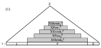
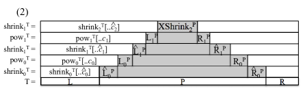
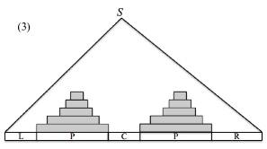
Figure 2: Abstract images of consistent signatures of substring $P$ of text $T$, on the derivation trees of the signature encoding of $T$. Gray rectangles in Figures (1)-(3) represent common signatures for occurrences of $P$. (1) Each $\mathit{XShrink}_{t}^{P}$ and $\mathit{XPow}_{t}^{P}$ occur on substring $P$ in $\mathit{shrink}_{t}^{T}$ and $\mathit{Pow}_{t}^{T}$, respectively, where $T=LPR$. (2) The substring $P$ can be represented by $\hat{L}_{0}^{P}L_{0}^{P}\hat{L}_{1}^{P}L_{1}^{P}\mathit{XShrink}_{2}^{P}R_{1}^{P}\hat{R}_{1}^{P}R_{0}^{P}\hat{R}_{0}^{P}$. (3) There exist common signatures on every substring $P$ in the derivation tree.

We give an intuitive description of Lemma 5. Recall that the locally consistent parsing of Lemma 4. Each $i$-th bit of bit sequence $d$ of Lemma 4 for a given string $s$ is determined by $s[i-\Delta_{L}..i+\Delta_{R}]$. Hence, for two positions $i,j$ such that $P=s[i..i+k-1]=s[j..j+k-1]$ for some $k$, $d[i+\Delta_{L}..i+k-1-\Delta_{R}]=d[j+\Delta_{L}..j+k-1-\Delta_{R}]$ holds, namely, “internal” bit sequences of the same substring of $s$ are equal. Since each level of the signature encoding uses the bit sequence, all occurrences of same substrings in a string share same internal signature sequences, and this goes up level by level. $\mathit{XShrink}_{t}^{P}$ and $\mathit{XPow}_{t}^{P}$ represent signature sequences which are obtained from only internal signature sequences of $\mathit{XPow}_{t-1}^{T}$ and $\mathit{XShrink}_{t}^{T}$, respectively. This means that $\mathit{XShrink}_{t}^{P}$ and $\mathit{XPow}_{t}^{P}$ are always created over $P$. From such common signatures we take as short signature sequence as possible for $\mathit{Uniq}(P)$: Since $\mathit{val}^{+}(\mathit{Pow}_{t-1}^{P})=\mathit{val}^{+}(L_{t-1}^{P}\mathit{XShrink}_{t}^{P}R_{t-1}^{P})$ and $\mathit{val}^{+}(\mathit{Shrink}_{t}^{P})=\mathit{val}^{+}(\hat{L}_{t}^{P}\mathit{XPow}_{t}^{P}\hat{R}_{t}^{P})$ hold, $|\mathit{Epow}(\mathit{Uniq}(P))|=O(\log|P|\log^{*}M)$ and $\mathit{val}^{+}(\mathit{Uniq}(P))=P$ hold. Hence Lemma 5 holds (see also Figure 2) .

From the common sequences we can derive many useful properties of signature encodings like listed below (see the references for proofs).

The number of ancestors of nodes corresponding to $\mathit{Uniq}(P)$ is upper bounded by:

Lemma 7 ([20]).

Let $\mathcal{G}$ be a signature encoding for a string $T$, $P$ be a string, and let $\mathcal{T}$ be the derivation tree of a signature $e\in\mathcal{V}$. Consider an occurrence of $P$ in $s$, and the induced subtree $X$ of $\mathcal{T}$ whose root is the root of $\mathcal{T}$ and whose leaves are the parents of the nodes representing $\mathit{Uniq}(P)$, where $s=\mathit{val}(e)$. Then $X$ contains $O(\log^{*}M)$ nodes for every level and $O(\log|s|+\log|P|\log^{*}M)$ nodes in total.

We can efficiently compute $\mathit{Uniq}(P)$ for a substring $P$ of $T$.

Lemma 8 ([20]).

Using a signature encoding $\mathcal{G}$ of size $w$, given a signature $e\in\mathcal{V}$ (and its corresponding node in the DAG) and two integers $j$ and $y$, we can compute $\mathit{Epow}(\mathit{Uniq}(s[j..j+y-1]))$ in $O(\log|s|+\log y\log^{*}M)$ time, where $s=\mathit{val}(e)$.

The next lemma shows that $\mathcal{G}$ requires only compressed space:

Lemma 9 ([23, 20]).

The size $w$ of the signature encoding of $T$ of length $N$ is $O(\min(z\log N\log^{*}M,N))$, where $z$ is the number of factors in the LZ77 factorization without self-reference of $T$.

The next lemma shows that the signature encoding supports (both forward and backward) LCE queries on a given arbitrary pair of signatures.

Lemma 10 ([20]).

Using a signature encoding $\mathcal{G}$ for a string $T$, we can support queries $\mathsf{LCE}(s_{1},s_{2},i,j)$ and $\mathsf{LCE}(s_{1}^{R},s_{2}^{R},i,j)$ in $O(\log|s_{1}|+\log|s_{2}|+\log\ell\log^{*}M)$ time for given two signatures $e_{1},e_{2}\in\mathcal{V}$ and two integers $1\leq i\leq|s_{1}|$, $1\leq j\leq|s_{2}|$, where $s_{1}=\mathit{val}(e_{1})$, $s_{2}=\mathit{val}(e_{2})$ and $\ell$ is the answer to the $\mathsf{LCE}$ query.

3.2 Dynamic signature encoding

We consider a dynamic signature encoding $\mathcal{G}$ of $T$, which allows for efficient updates of $\mathcal{G}$ in compressed space according to the following operations: $\mathit{INSERT}(Y,i)$ inserts a string $Y$ into $T$ at position $i$, i.e., $T\leftarrow T[..i-1]YT[i..]$; $\mathit{INSERT^{\prime}}(j,y,i)$ inserts $T[j..j+y-1]$ into $T$ at position $i$, i.e., $T\leftarrow T[..i-1]T[j..j+y-1]T[i..]$; and $\mathit{DELETE}(j,y)$ deletes a substring of length $y$ starting at $j$, i.e., $T\leftarrow T[..j-1]T[j+y..]$.

During updates we recompute $\mathit{Shrink}_{t}^{T}$ and $\mathit{Pow}_{t}^{T}$ for some part of new $T$ (note that the most part is unchanged thanks to the virtue of signature encodings, Lemma 7). When we need a signature for $\mathit{expr}$, we look up the signature assigned to $\mathit{expr}$ (i.e., compute $\mathit{Assign}^{-1}(\mathit{expr})$) and use it if such exists. If $\mathit{Assign}^{-1}(\mathit{expr})$ is undefined we create a new signature $e_{\mathit{new}}$, which is an integer that is currently not used as signatures, and add $e_{\mathit{new}}\rightarrow\mathit{expr}$ to $\mathcal{D}$. Also, updates may produce a useless signature whose parents in the DAG are all removed. We remove such useless signatures from $\mathcal{G}$ during updates.

We can upper bound the number of signatures added to or removed from $\mathcal{G}$ after a single update operation by the following lemma.

Lemma 11.

After $\mathit{INSERT}(Y,i)$ or $\mathit{DELETE}(j,y)$ operation, $O(y+\log N\log^{*}M)$ signatures are added to or removed from $\mathcal{G}$, where $|Y|=y$. After $\mathit{INSERT^{\prime}}(j,y,i)$ operation, $O(\log N\log^{*}M)$ signatures are added to or removed from $\mathcal{G}$.

Proof.

Consider $\mathit{INSERT^{\prime}}(j,y,i)$ operation. Let $T^{\prime}=T[..i-1]T[j..j+y-1]T[i..]$ be the new text. Note that by Lemma 5 the signature encoding of $T^{\prime}$ is created over $\mathit{Uniq}(T[..i-1])\mathit{Uniq}(T[j..j+y-1])\mathit{Uniq}(T[i..])$, and hence, $O(\log N\log^{*}M)$ signatures can be added by Lemma 7. Also, $O(\log N\log^{*}M)$ signatures, which were created over $\mathit{Uniq}(T[..i-1])\mathit{Uniq}(T[i..])$, may be removed.

For $\mathit{INSERT}(Y,i)$ operation, we additionally think about the possibility that $O(y)$ signatures are added to create $\mathit{Uniq}(Y)$. Similarly, for $\mathit{DELETE}(j,y)$ operation, $O(y)$ signatures, which are used in and under $\mathit{Uniq}(T[j..j+y-1])$, can be removed. ∎∎

In [20], it was shown how to augment the DAG representation of $\mathcal{G}$ to add/remove an assignment to/from $\mathcal{G}$ in $O(f_{\mathcal{A}})$ time, where $f_{\mathcal{A}}=O\left(\min\left\{\frac{\log\log M\log\log w}{\log\log\log M},\sqrt{\frac{\log w}{\log\log w}}\right\}\right)$ is the time complexity of Beame and Fich’s data structure [4] to support predecessor/successor queries on a set of $w$ integers from an $M$-element universe. Note that there is a small difference in our DAG representation from the one in [20]; our DAG has a doubly-linked list representing the parents of a node. We can check if a signature is useless or not by checking if the list is empty or not, and the lists can be maintained in constant time after adding/removing an assignment. Hence, the next lemma still holds for our DAG representation.

Lemma 12 (Dynamic signature encoding [20]).

After processing $\mathcal{G}$ in $O(wf_{\mathcal{A}})$ time, we can insert/delete any (sub)string $Y$ of length $y$ into/from an arbitrary position of $T$ in $O((y+\log N\log^{*}M)f_{\mathcal{A}})$ time. Moreover, if $Y$ is given as a substring of $T$, we can support insertion in $O(f_{\mathcal{A}}\log N\log^{*}M)$ time.

4 Dynamic Compressed Index

In this section, we present our dynamic compressed index based on signature encoding. As already mentioned in the introduction, our strategy for pattern matching is different from that of Alstrup et al. [2]. It is rather similar to the one taken in the static index for SLPs of Claude and Navarro [6]. Besides applying their idea to RLSLPs, we show how to speed up pattern matching by utilizing the properties of signature encodings. Index for SLPs. Here we review how the index in [6] for SLP $\mathcal{S}$ generating a string $T$ computes $\mathit{Occ}(P,T)$ for a given string $P$. The key observation is that, any occurrence of $P$ in $T$ can be uniquely associated with the lowest node that covers the occurrence of $P$ in the derivation tree. As the derivation tree is binary, if $|P|>1$, then the node is labeled with some variable $X\in\mathcal{V}$ such that $P_{1}$ is a suffix of $X.{\rm left}$ and $P_{2}$ is a prefix of $X.{\rm right}$, where $P=P_{1}P_{2}$ with $1\leq|P_{1}|<|P|$. Here we call the pair $(X,|X.{\rm left}|-|P_{1}|+1)$ a primary occurrence of $P$, and let $\mathit{pOcc}_{\mathcal{S}}(P,j)$ denote the set of such primary occurrences with $|P_{1}|=j$. The set of all primary occurrences is denoted by $\mathit{pOcc}_{\mathcal{S}}(P)=\bigcup_{1\leq j<|P|}\mathit{pOcc}_{\mathcal{S}}(P,j)$. Then, we can compute $\mathit{Occ}(P,T)$ by first computing primary occurrences and enumerating the occurrences of $X$ in the derivation tree.

The set $\mathit{Occ}(P,T)$ of occurrences of $P$ in $T$ is represented by $\mathit{pOcc}_{\mathcal{S}}(P)$ as follows: $\mathit{Occ}(P,T)=\{j+k-1\mid(X,j)\in\mathit{pOcc}_{\mathcal{S}}(P),k\in\mathit{vOcc}(X,S)\}$ if $|P|>1$; $\mathit{Occ}(P,T)=\mathit{vOcc}(X,S)((X\rightarrow P)\in\mathcal{D})$ if $|P|=1$. See also Example 27.

Hence the task is to compute $\mathit{pOcc}_{\mathcal{S}}(P)$ and $\mathit{vOcc}(X,S)$ efficiently. Note that $\mathit{vOcc}(X,S)$ can be computed in $O(|\mathit{vOcc}(X,S)|h)$ time by traversing the DAG in a reversed direction from $X$ to the source, where $h$ is the height of the derivation tree of $S$. Hence, in what follows, we explain how to compute $\mathit{pOcc}_{\mathcal{S}}(P)$ for a string $P$ with $|P|>1$. We consider the following problem:

Problem 13 (Two-Dimensional Orthogonal Range Reporting Problem).

Let $\mathcal{X}$ and $\mathcal{Y}$ denote subsets of two ordered sets, and let $\mathcal{R}\subseteq\mathcal{X}\times\mathcal{Y}$ be a set of points on the two-dimensional plane, where $|\mathcal{X}|,|\mathcal{Y}|\in O(|\mathcal{R}|)$. A data structure for this problem supports a query $\mathit{report}_{\mathcal{R}}(x_{1},x_{2},y_{1},y_{2})$; given a rectangle $(x_{1},x_{2},y_{1},y_{2})$ with $x_{1},x_{2}\in\mathcal{X}$ and $y_{1},y_{2}\in\mathcal{Y}$, returns $\{(x,y)\in\mathcal{R}\mid x_{1}\leq x\leq x_{2},y_{1}\leq y\leq y_{2}\}$.

Data structures for Problem 13 are widely studied in computational geometry. There is even a dynamic variant, which we finally use for our dynamic index. Until then, we just use any data structure that occupies $O(|\mathcal{R}|)$ space and supports queries in $O(\hat{q}_{|\mathcal{R}|}+q_{|\mathcal{R}|}\mathit{qocc})$ time with $\hat{q}_{|\mathcal{R}|}=O(\log|\mathcal{R}|)$, where $\mathit{qocc}$ is the number of points to report.

Now, given an SLP $\mathcal{S}$, we consider a two-dimensional plane defined by $\mathcal{X}=\{X.{\rm left}^{R}\mid X\in\mathcal{V}\}$ and $\mathcal{Y}=\{X.{\rm right}\mid X\in\mathcal{V}\}$, where elements in $\mathcal{X}$ and $\mathcal{Y}$ are sorted by lexicographic order. Then consider a set of points $\mathcal{R}=\{(X.{\rm left}^{R},X.{\rm right})\mid X\in\mathcal{V}\}$. For a string $P$ and an integer $1\leq j<|P|$, let $y_{1}^{(P,j)}$ (resp. $y_{2}^{(P,j)}$) denote the lexicographically smallest (resp. largest) element in $\mathcal{Y}$ that has $P[j+1..]$ as a prefix. If there is no such element, it just returns NIL and we can immediately know that $\mathit{pOcc}_{\mathcal{S}}(P,j)=\emptyset$. We define $x_{1}^{(P,j)}$ and $x_{2}^{(P,j)}$ in a similar way over $\mathcal{X}$. Then, $\mathit{pOcc}_{\mathcal{S}}(P,j)$ can be computed by a query $\mathit{report}_{\mathcal{R}}(x_{1}^{(P,j)},x_{2}^{(P,j)},y_{1}^{(P,j)},y_{2}^{(P,j)})$ (see also Example 28).

Using this idea, we can get the next result:

Lemma 14.

For an SLP $\mathcal{S}$ of size $n$, there exists a data structure of size $O(n)$ that computes, given a string $P$, $\mathit{pOcc}_{\mathcal{S}}(P)$ in $O(|P|(h+|P|)\log n+q_{n}|\mathit{pOcc}_{\mathcal{S}}(P)|)$ time.

Proof.

For every $1\leq j<|P|$, we compute $\mathit{pOcc}_{\mathcal{S}}(P,j)$ by $\mathit{report}_{\mathcal{R}}(x_{1}^{(P,j)},x_{2}^{(P,j)},y_{1}^{(P,j)},y_{2}^{(P,j)})$. We can compute $y_{1}^{(P,j)}$ and $y_{2}^{(P,j)}$ in $O((h+|P|)\log n)$ time by binary search on $\mathcal{Y}$, where each comparison takes $O(h+|P|)$ time for expanding the first $O(|P|)$ characters of variables subjected to comparison. In a similar way, $x_{1}^{(P,j)}$ and $x_{2}^{(P,j)}$ can be computed in $O((h+|P|)\log n)$ time. Thus, the total time complexity is $O(|P|((h+|P|)\log n+\hat{q}_{n})+q_{n}|\mathit{pOcc}_{\mathcal{S}}(P)|)=O(|P|(h+|P|)\log n+q_{n}|\mathit{pOcc}_{\mathcal{S}}(P)|)$. ∎∎

Index for RLSLPs. We extend the idea for the SLP index described above to RLSLPs. The difference from SLPs is that we have to deal with occurrences of $P$ that are covered by a node labeled with $X\rightarrow\hat{X}^{k}$ but not covered by any single child of the node in the derivation tree. In such a case, there must exist $P=P_{1}P_{2}$ with $1\leq|P_{1}|<|P|$ such that $P_{1}$ is a suffix of $X.{\rm left}=\mathit{val}^{+}(\hat{X})$ and $P_{2}$ is a prefix of $X.{\rm right}=\mathit{val}^{+}(\hat{X}^{k-1})$. Let $j=|\mathit{val}(\hat{X})|-|P_{1}|+1$ be a position in $\mathit{val}^{+}(\hat{X}^{d})$ where $P$ occurs, then $P$ also occurs at $j+c|\mathit{val}(\hat{X})|$ in $\mathit{val}^{+}(\hat{X}^{k})$ for every positive integer $c$ with $j+c|\mathit{val}(\hat{X})|+|P|-1\leq|\mathit{val}^{+}(\hat{X}^{k})|$. Using this observation, the index for SLPs can be modified for RLSLPs to achieve the same bounds as in Lemma 14. Index for signature encodings. Since signature encodings are RLSLPs, we can compute $\mathit{Occ}(P,T)$ by querying $\mathit{report}_{\mathcal{R}}(x_{1}^{(P,j)},x_{2}^{(P,j)},y_{1}^{(P,j)},y_{2}^{(P,j)})$ for “every” $1\leq j<|P|$. However, the properties of signature encodings allow us to speed up pattern matching as summarized in the following two ideas: (1) We can efficiently compute $x_{1}^{(P,j)},x_{2}^{(P,j)},y_{1}^{(P,j)}$ and $y_{2}^{(P,j)}$ using LCE queries in compressed space (Lemma 15). (2) We can reduce the number of $\mathit{report}_{\mathcal{R}}$ queries from $O(|P|)$ to $O(\log|P|\log^{*}M)$ by using the property of the common sequence of $P$ (Lemma 16).

Lemma 15.

Assume that we have the signature encoding $\mathcal{G}$ of size $w$ for a string $T$ of length $N$, $\mathcal{X}$ and $\mathcal{Y}$ of $\mathcal{G}$. Given a signature $\mathit{id}(P)\in\mathcal{V}$ for a string $P$ and an integer $j$, we can compute $x_{1}^{(P,j)},x_{2}^{(P,j)},y_{1}^{(P,j)}$ and $y_{2}^{(P,j)}$ in $O(\log w(\log N+\log|P|\log^{*}M))$ time.

Proof.

By Lemma 10 we can compute $x_{1}^{(P,j)}$ and $x_{2}^{(P,j)}$ on $\mathcal{X}$ by binary search in $O(\log w(\log N+\log|P|\log^{*}M))$ time. Similarly, we can compute $y_{1}^{(P,j)}$ and $y_{2}^{(P,j)}$ in the same time. ∎∎

Lemma 16.

Let $P$ be a string with $|P|>1$. If $|\mathit{Pow}_{0}^{P}|=1$, then $\mathit{pOcc}_{\mathcal{G}}(P)=\mathit{pOcc}_{\mathcal{G}}(P,1)$. If $|\mathit{Pow}_{0}^{P}|>1$, then $\mathit{pOcc}_{\mathcal{G}}(P)=\bigcup_{j\in\mathcal{P}}\mathit{pOcc}_{\mathcal{G}}(P,j)$, where $\mathcal{P}=\{|\mathit{val}^{+}(u[1..i])|\mid 1\leq i<|u|,u[i]\neq u[i+1]\}$ with $u=\mathit{Uniq}(P)$.

Proof.

If $|\mathit{Pow}_{0}^{P}|=1$, then $P=a^{|P|}$ for some character $a\in\Sigma$. In this case, $P$ must be contained in a node labeled with a signature $e\rightarrow\hat{e}^{d}$ such that $\hat{e}\rightarrow a$ and $d\geq|P|$. Hence, all primary occurrences of $P$ can be found by $\mathit{pOcc}_{\mathcal{G}}(P,1)$.

If $|\mathit{Pow}_{0}^{P}|>1$, we consider the common sequence $u$ of $P$. Recall that substring $P$ occurring at $j$ in $\mathit{val}(e)$ is represented by $u$ for any $(e,j)\in\mathit{pOcc}(P)$ by Lemma 5 Hence at least $\mathit{pOcc}_{\mathcal{G}}(P)=\bigcup_{i\in\mathcal{P^{\prime}}}\mathit{pOcc}_{\mathcal{G}}(P,i)$ holds, where $\mathcal{P^{\prime}}=\{|\mathit{val}^{+}(u[1])|,\ldots,|\mathit{val}^{+}(u[..|u|-1])|\}$. Moreover, we show that $\mathit{pOcc}_{\mathcal{G}}(P,i)=\emptyset$ for any $i\in\mathcal{P^{\prime}}$ with $u[i]=u[i+1]$. Note that $u[i]$ and $u[i+1]$ are encoded into the same signature in the derivation tree of $e$, and that the parent of two nodes corresponding to $u[i]$ and $u[i+1]$ has a signature $e^{\prime}$ in the form $e^{\prime}\rightarrow u[i]^{d}$. Now assume for the sake of contradiction that $e=e^{\prime}$. By the definition of the primary occurrences, $i=1$ must hold, and hence, $\mathit{Shrink}_{0}^{P}[1]=u[1]\in\Sigma$. This means that $P=u[1]^{|P|}$, which contradicts $|\mathit{Pow}_{0}^{P}|>1$. Therefore the statement holds. ∎∎

Using Lemmas 5, 15 and 16, we get a static index for signature encodings:

Lemma 17.

For a signature encoding $\mathcal{G}$ of size $w$ which generates a text $T$ of length $N$, there exists a data structure of size $O(w)$ that computes, given a string $P$, $\mathit{pOcc}_{\mathcal{G}}(P)$ in $O(|P|f_{\mathcal{A}}+\log w\log|P|\log^{*}M(\log N+\log|P|\log^{*}M)+q_{w}|\mathit{pOcc}_{\mathcal{S}}(P)|)$ time.

Proof.

We focus on the case $|\mathit{Pow}_{0}^{P}|>1$ as the other case is easier to be solved. We first compute the common sequence of $P$ in $O(|P|f_{\mathcal{A}})$ time. Taking $\mathcal{P}$ in Lemma 16, we recall that $|\mathcal{P}|=O(\log|P|\log^{*}M)$ by Lemma 5. Then, in light of Lemma 16, $\mathit{pOcc}_{\mathcal{G}}(P)$ can be obtained by $|\mathcal{P}|=O(\log|P|\log^{*}M)$ range reporting queries. For each query, we spend $O(\log w(\log N+\log|P|\log^{*}M))$ time to compute $x_{1}^{(P,j)},x_{2}^{(P,j)},y_{1}^{(P,j)}$ and $y_{2}^{(P,j)}$ by Lemma 15. Hence, the total time complexity is

$$O(|P|f_{\mathcal{A}}+\log|P|\log^{*}M(\log w(\log N+\log|P|\log^{*}M)+\hat{q}_{w})+q_{w}|\mathit{pOcc}_{\mathcal{S}}(P)|)$$

$$=O(|P|f_{\mathcal{A}}+\log w\log|P|\log^{*}M(\log N+\log|P|\log^{*}M)+q_{w}|\mathit{pOcc}_{\mathcal{S}}(P)|).$$

∎∎

In order to dynamize our index of Lemma 17, we consider a data structure for “dynamic” two-dimensional orthogonal range reporting that can support the following update operations:

• $\mathit{insert}_{\mathcal{R}}(p,x_{\mathit{pred}},y_{\mathit{pred}})$: given a point $p=(x,y)$, $x_{\mathit{pred}}=\max\{x^{\prime}\in\mathcal{X}\mid x^{\prime}\leq x\}$ and $y_{\mathit{pred}}=\max\{y^{\prime}\in\mathcal{Y}\mid y^{\prime}\leq y\}$, insert $p$ to $\mathcal{R}$ and update $\mathcal{X}$ and $\mathcal{Y}$ accordingly.

• $\mathit{delete}_{\mathcal{R}}(p)$: given a point $p=(x,y)\in\mathcal{R}$, delete $p$ from $\mathcal{R}$ and update $\mathcal{X}$ and $\mathcal{Y}$ accordingly.

We use the following data structure for the dynamic two-dimensional orthogonal range reporting.

Lemma 18 ([5]).

There exists a data structure that supports $\mathit{report}_{\mathcal{R}}(x_{1},x_{2},y_{1},y_{2})$ in $O(\log|\mathcal{R}|+\mathit{occ}(\log|\mathcal{R}|/\log\log|\mathcal{R}|))$ time, and $\mathit{insert}_{\mathcal{R}}(p,i,j)$, $\mathit{delete}_{\mathcal{R}}(p)$ in amortized $O(\log|\mathcal{R}|)$ time, where $\mathit{occ}$ is the number of the elements to output. This structure uses $O(|\mathcal{R}|)$ space. 

Proof of Theorem 1.

Our index consists of a dynamic signature encoding $\mathcal{G}$ and a dynamic range reporting data structure of Lemma 18 whose $\mathcal{R}$ is maintained as they are defined in the static version. We maintain $\mathcal{X}$ and $\mathcal{Y}$ in two ways; self-balancing binary search trees for binary search, and Dietz and Sleator’s data structures for order maintenance. Then, primary occurrences of $P$ can be computed as described in Lemma 17. Adding the $O(\mathit{occ}\log N)$ term for computing all pattern occurrences from primary occurrences, we get the time complexity for pattern matching in the statement.

Concerning the update of our index, we described how to update $\mathcal{G}$ after $\mathit{INSERT}$, $\mathit{INSERT^{\prime}}$ and $\mathit{DELETE}$ in Lemma 12. What remains is to show how to update the dynamic range reporting data structure when a signature is added to or deleted from $\mathcal{V}$. When a signature $e$ is deleted from $\mathcal{V}$, we first locate $e.{\rm left}^{R}$ on $\mathcal{X}$ and $e.{\rm right}$ on $\mathcal{Y}$, and then execute $\mathit{delete}_{\mathcal{R}}(e.{\rm left}^{R},e.{\rm right})$. When a signature $e$ is added to $\mathcal{V}$, we first locate $x_{\mathit{pred}}=\max\{x^{\prime}\in\mathcal{X}\mid x^{\prime}\leq e.{\rm left}^{R}\}$ on $\mathcal{X}$ and $y_{\mathit{pred}}=\max\{y^{\prime}\in\mathcal{Y}\mid y^{\prime}\leq e.{\rm right}\}$ on $\mathcal{Y}$, and then execute $\mathit{insert}_{\mathcal{R}}((e.{\rm left}^{R},e.{\rm right}),x_{\mathit{pred}},y_{\mathit{pred}})$. The locating can be done by binary search on $\mathcal{X}$ and $\mathcal{Y}$ in $O(\log w\log N\log^{*}M)$ time as Lemma 15.

Since the number of signatures added to or removed from $\mathcal{G}$ during a single update operation is upper bounded by Lemma 11, we can get the desired time bounds of Theorem 1. ∎∎

5 LZ77 factorization in compressed space

In this section, we show Theorem 3. Note that since each $f_{i}$ can be represented by the pair $(x_{i},|f_{i}|)$, we compute incrementally $(x_{i},|f_{i}|)$ in our algorithm, where $x_{i}$ is an occurrence position of $f_{i}$ in $f_{1}\cdots f_{i-1}$.

For integers $j,k$ with $1\leq j\leq j+k-1\leq N$, let $\mathit{Fst}(j,k)$ be the function which returns the minimum integer $i$ such that $i<j$ and $T[i..i+k-1]=T[j..j+k-1]$, if it exists. Our algorithm is based on the following fact:

Fact 19.

Let $f_{1},\ldots,f_{z}$ be the LZ77-factorization of a string $T$. Given $f_{1},\ldots,f_{i-1}$, we can compute $f_{i}$ with $O(\log|f_{i}|)$ calls of $\mathit{Fst}(j,k)$ (by doubling the value of $k$, followed by a binary search), where $j=|f_{1}\cdots f_{i-1}|+1$.

We explain how to support queries $\mathit{Fst}(j,k)$ using the signature encoding. We define $e.{\rm min}=\min\mathit{vOcc}(e,S)+|e.{\rm left}|$ for a signature $e\in\mathcal{V}$ with $e\rightarrow e_{\ell}e_{r}$ or $e\rightarrow\hat{e}^{k}$. We also define $\mathit{FstOcc}(P,i)$ for a string $P$ and an integer $i$ as follows:

$$\mathit{FstOcc}(P,i)=\min\{e.{\rm min}\mid(e,i)\in\mathit{pOcc}_{\mathcal{G}}(P,i)\}$$

Then $\mathit{Fst}(j,k)$ can be represented by $\mathit{FstOcc}(P,i)$ as follows:

$$\mathit{Fst}(j,k) = \min\{\mathit{FstOcc}(T[j..j+k-1],i)-i\mid i\in\{1,\ldots,k-1\}$$

$$= \min\{\mathit{FstOcc}(T[j..j+k-1],i)-i\mid i\in\mathcal{P}\},$$

where $\mathcal{P}$ is the set of integers in Lemma 16 with $P=T[j..j+k-1]$.

Recall that in Section 4 we considered the two-dimensional orthogonal range reporting problem to enumerate $\mathit{pOcc}_{\mathcal{G}}(P,i)$. Note that $\mathit{FstOcc}(P,i)$ can be obtained by taking $(e,i)\in\mathit{pOcc}_{\mathcal{G}}(P,i)$ with $e.{\rm min}$ minimum. In order to compute $\mathit{FstOcc}(P,i)$ efficiently instead of enumerating all elements in $\mathit{pOcc}_{\mathcal{G}}(P,i)$, we give every point corresponding to $e$ the weight $e.{\rm min}$ and use the next data structure to compute a point with the minimum weight in a given rectangle.

Lemma 20 ([1]).

Consider $n$ weighted points on a two-dimensional plane. There exists a data structure which supports the query to return a point with the minimum weight in a given rectangle in $O(\log^{2}n)$ time, occupies $O(n)$ space, and requires $O(n\log n)$ time to construct.

Using Lemma 20, we get the following lemma.

Lemma 21.

Given a signature encoding $\mathcal{G}$ of size $w$ which generates $T$, we can construct a data structure of $O(w)$ space in $O(w\log w\log N\log^{*}M)$ time to support queries $\mathit{Fst}(j,k)$ in $O(\log w\log k\log^{*}M(\log N+\log k\log^{*}M))$ time.

Proof.

For construction, we first compute $e.{\rm min}$ in $O(w)$ time using the DAG of $\mathcal{G}$. Next, we prepare the plane defined by the two ordered sets $\mathcal{X}$ and $\mathcal{Y}$ in Section 4. This can be done in $O(w\log w\log N\log^{*}M)$ time by sorting elements in $\mathcal{X}$ (and $\mathcal{Y}$) by $\mathsf{LCE}$ algorithm (Lemma 10) and a standard comparison-based sorting. Finally we build the data structure of Lemma 20 in $O(w\log w)$ time.

To support a query $\mathit{Fst}(j,k)$, we first compute $\mathit{Epow}(\mathit{Uniq}(P))$ with $P=T[j..j+k-1]$ in $O(\log N+\log k\log^{*}M)$ time by Lemma 8, and then get $\mathcal{P}$ in Lemma 16. Since $|\mathcal{P}|=O(\log k\log^{*}M)$ by Lemma 5, $\mathit{Fst}(j,k)=\min\{\mathit{FstOcc}(P,i)-i\mid i\in\mathcal{P}\}$ can be computed by answering $\mathit{FstOcc}$ $O(\log k\log^{*}M)$ times. For each computation of $\mathit{FstOcc}(P,i)$, we spend $O(\log w(\log N+\log k\log^{*}M))$ time to compute $x_{1}^{(P,j)},x_{2}^{(P,j)},y_{1}^{(P,j)}$ and $y_{2}^{(P,j)}$ by Lemma 15, and $O(\log^{2}w)$ time to compute a point with the minimum weight in the rectangle $(x_{1}^{(P,j)},x_{2}^{(P,j)},y_{1}^{(P,j)},y_{2}^{(P,j)})$. Hence it takes $O(\log k\log^{*}M(\log w(\log N+\log k\log^{*}M)+\log^{2}w))=O(\log w\log k\log^{*}M(\log N+\log k\log^{*}M))$ time in total. ∎∎

We are ready to prove Theorem 3 holds.

Proof of Theorem 3.

We compute the $z$ factors of the LZ77-factorization of $T$ incrementally by using Fact 19 and Lemma 21 in $O(z\log w\log^{3}N(\log^{*}M)^{2})$ time. Therefore the statement holds. ∎∎

We remark that we can similarly compute the Lempel-Ziv77 factorization with self-reference of a text (defined below) in the same time and same working space.

Definition 22 (Lempel-Ziv77 factorization with self-reference [29]).

The Lempel-Ziv77 (LZ77) factorization of a string $s$ with self-references is a sequence $f_{1},\ldots,f_{k}$ of non-empty substrings of $s$ such that $s=f_{1}\cdots f_{k}$, $f_{1}=s[1]$, and for $1<i\leq k$, if the character $s[|f_{1}..f_{i-1}|+1]$ does not occur in $s[|f_{1}..f_{i-1}|]$, then $f_{i}=s[|f_{1}..f_{i-1}|+1]$, otherwise $f_{i}$ is the longest prefix of $f_{i}\cdots f_{k}$ which occurs at some position $p$, where $1\leq p\leq|f_{1}\cdots f_{i-1}|$.

Acknowledgments. We would like to thank Paweł Gawrychowski for drawing our attention to the work by Alstrup et al. [2, 3] and for fruitful discussions.

Appendix A Appendix: Supplementary Examples and Figures

Example 23 ($\mathit{Eblock}_{d}(p)$ and $\mathit{Epow}(s)$).

Let $\log^{*}W=2$, and then $\Delta_{L}=8,\Delta_{R}=4$.
If $p=1,2,3,2,5,7,6,4,3,4,3,4,1,2,3,4,5$ and $d=1,0,0,1,0,1,0,0,1,0,0,0,1,0,1,0,0$, then $\mathit{Eblock}_{d}(p)=(1,2,3),(2,5),(7,6,4),(3,4,3,4),(1,2),(3,4,5)$, $|\mathit{Eblock}_{d}(p)|=6$ and $\mathit{Eblock}_{d}(p)[2]=(2,5)$. For string $s=aaaabbbbbabbaa$, $\mathit{Epow}(s)=a^{4}b^{5}a^{1}b^{2}a^{2}$ and $|\mathit{Epow}(s)|=5$ and $\mathit{Epow}(s)[2]=b^{5}$.

Example 24 (SLP).

Let $\mathcal{S}=(\Sigma,\mathcal{V},\mathcal{D},S)$ be the SLP s.t. $\Sigma=\{A,B,C\}$, $\mathcal{V}=\{X_{1},\cdots,X_{11}\}$, $\mathcal{D}=\{X_{1}\rightarrow A,X_{2}\rightarrow B,X_{3}\rightarrow C,X_{4}\rightarrow X_{3}X_{1},X_{5}\rightarrow X_{4}X_{2},X_{6}\rightarrow X_{5}X_{5},X_{7}\rightarrow X_{2}X_{3},X_{8}\rightarrow X_{1}X_{2},X_{9}\rightarrow X_{7}X_{8},X_{10}\rightarrow X_{6}X_{9},X_{11}\rightarrow X_{10}X_{6}\}$, $S=X_{11}$, the derivation tree of $S$ represents $CABCABBCABCABCAB$.

Example 25 (RLSLP).

Let $\mathcal{G}=(\Sigma,\mathcal{V},\mathcal{D},S)$ be an RLSLP, where $\Sigma=\{A,B\}$, $\mathcal{V}=\{1,\ldots,24\}$, $\mathcal{D}=\{1\rightarrow A,2\rightarrow B,3\rightarrow 1^{1},4\rightarrow 2^{1},5\rightarrow 2^{2},6\rightarrow 1^{2},7\rightarrow(3,4),8\rightarrow(3,5),9\rightarrow(8,3),10\rightarrow(4,3),11\rightarrow(10,4),12\rightarrow(11,6),13\rightarrow 7^{3},14\rightarrow 9^{1},15\rightarrow 10^{1},16\rightarrow 12^{1},17\rightarrow 10^{3},18\rightarrow(13,14),19\rightarrow(18,15),20\rightarrow(16,17),21\rightarrow 19^{1},22\rightarrow 20^{1},23\rightarrow(21,22),24\rightarrow 23^{1}\}$, and $S=24$. The derivation tree of the start symbol $S$ represents a single string $T=ABABABABBABABABAABABABA$.

Example 26 (Signature encoding).

Let $\mathcal{G}=(\Sigma,\mathcal{V},\mathcal{D},S)$ be an RLSLP of Example 25. Assuming $\mathit{Eblock}(\mathit{Pow}_{0}^{T})=(3,4)^{3},(3,5,3),(4,3),(4,3,4,6),(4,3)^{3}$, $\mathit{Eblock}(\mathit{Pow}_{2}^{T})=(13,14,15),(16,17)$ and $\mathit{Eblock}(\mathit{Pow}_{3}^{T})=(21,22)$ hold, $\mathcal{G}$ is the signature encoding of $T$ and $\mathit{id}(T)=24$. Here, $\mathit{Sig}((13,14))=18$, $\mathit{Sig}((4,3,4,6))=12$, $\mathit{Sig}((4,5))=\rm{undefined}$. See Fig. 1 for an illustration of the derivation tree of $\mathcal{G}$ and the corresponding DAG.

Example 27 (Primary occurrences).

Let $\mathcal{S}$ be the SLP of Example 24. Given a pattern $P=BCAB$, then $P$ occurs at $3$, $7$, $10$ and $13$ in the string $T$ represented by SLP $\mathcal{S}$. Hence $\mathit{Occ}(P,T)=\{3,7,10,13\}$. On the other hand, $P$ occurs at $3$ in $\mathit{val}(X_{6})$ and $P$ is divided by $X_{5}$ and $X_{5}$, where $X_{6}\rightarrow X_{5}X_{5}$. Similarly, divided $P$ occurs at $1$ in $\mathit{val}(X_{9})$, at $10$ in $\mathit{val}(X_{11})$. Hence $\mathit{pOcc}_{\mathcal{S}}(P)=\{(X_{6},3),(X_{11},10),(X_{9},1)\}$. Specifically $\mathit{pOcc}_{\mathcal{S}}(P,1)=\{(X_{6},3),(X_{11},10)\}$, $\mathit{pOcc}_{\mathcal{S}}(P,2)=\{(X_{9},1)\}$ and $\mathit{pOcc}_{\mathcal{S}}(P,3)=\phi$. Hence we can also compute $\mathit{Occ}(P,T)=\{3,7,10,13\}$ by $\mathit{vOcc}(X_{6},S)=\{1,11\}$, $\mathit{vOcc}(X_{9},S)=\{7\}$, and $\mathit{vOcc}(X_{11},S)=\{1\}$. See also Fig. 3.

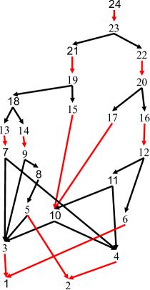
Figure 1: The derivation tree of $S$ (left) and the DAG for $\mathcal{G}$ (right) of Example 25. In the DAG, the black and red arrows represent $e\rightarrow e_{\ell}e_{r}$ and $e\rightarrow\hat{e}^{k}$ respectively. In Example 26, $T$ is encoded by signature encoding.

Example 28 (SLP).

Let $\mathcal{S}$ be the SLP of Example 24. Then,

$$\mathcal{X} = \{x_{1},x_{4},x_{2},x_{8},x_{5},x_{9},x_{6},x_{10},x_{11},x_{3},x_{7}\},$$

$$\mathcal{Y} = \{y_{1},y_{8},y_{2},y_{7},y_{9},y_{3},y_{4},y_{5},y_{6},y_{10},y_{11}\},$$

$x_{i}=\mathit{val}(X_{i})^{R}$, $y_{i}=\mathit{val}(X_{i})$ for any $X_{i}\in\mathcal{V}$. See also Fig. 3.

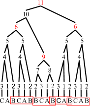
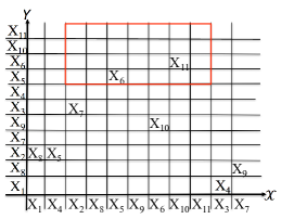
Figure 3: The left figure is the derivation tree of SLP $\mathcal{S}$ of Example 24, which derives the string $T$. The red rectangles on $T$ represent all occurrences of $P=BCAB$ in $T$. The right grid represents the relation between $\mathcal{X}$, $\mathcal{Y}$ and $\mathcal{R}$ of Example 28. The red rectangle on the grid is a query rectangle $(x^{(P,1)}_{1},x^{(P,1)}_{2},y^{(P,1)}_{1},y^{(P,1)}_{2})$, where $x^{(P,1)}_{1}=x_{2}$, $x^{(P,1)}_{2}=x_{11}$, $y^{(P,1)}_{1}=y_{5}$ and $y^{(P,1)}_{2}=y_{11}$. Therefore, $\mathit{report}_{\mathcal{R}}(x^{(P,1)}_{1},x^{(P,1)}_{2},y^{(P,1)}_{1},y^{(P,1)}_{2})=\{X_{6},X_{11}\}$.

References

- [1] P. K. Agarwal, L. Arge, S. Govindarajan, J. Yang, and K. Yi, Efficient external memory structures for range-aggregate queries, Comput. Geom., 46 (2013), pp. 358–370.
- [2] S. Alstrup, G. S. Brodal, and T. Rauhe, Dynamic pattern matching, tech. rep., Department of Computer Science, University of Copenhagen, 1998.
- [3] , Pattern matching in dynamic texts, in Proc. SODA 2000, 2000, pp. 819–828.
- [4] P. Beame and F. E. Fich, Optimal bounds for the predecessor problem and related problems, J. Comput. Syst. Sci., 65 (2002), pp. 38–72.
- [5] G. E. Blelloch, Space-efficient dynamic orthogonal point location, segment intersection, and range reporting, in SODA, S.-H. Teng, ed., SIAM, 2008, pp. 894–903.
- [6] F. Claude and G. Navarro, Self-indexed grammar-based compression, Fundamenta Informaticae, 111 (2011), pp. 313–337.
- [7] , Improved grammar-based compressed indexes, in SPIRE’12, 2012, pp. 180–192.
- [8] P. F. Dietz and D. D. Sleator, Two algorithms for maintaining order in a list, in Proceedings of the 19th Annual ACM Symposium on Theory of Computing, 1987, New York, New York, USA, A. V. Aho, ed., ACM, 1987, pp. 365–372.
- [9] A. Ehrenfeucht, R. M. McConnell, N. Osheim, and S. Woo, Position heaps: A simple and dynamic text indexing data structure, J. Discrete Algorithms, 9 (2011), pp. 100–121.
- [10] J. Fischer, T. Gagie, P. Gawrychowski, and T. Kociumaka, Approximating LZ77 via small-space multiple-pattern matching, in ESA 2015, 2015, pp. 533–544.
- [11] T. Gagie, P. Gawrychowski, J. Kärkkäinen, Y. Nekrich, and S. J. Puglisi, A faster grammar-based self-index, in LATA’12, 2012, pp. 240–251.
- [12] T. Gagie, P. Gawrychowski, J. Kärkkäinen, Y. Nekrich, and S. J. Puglisi, LZ77-based self-indexing with faster pattern matching, in Proc. LATIN 2014, 2014, pp. 731–742.
- [13] T. Gagie, P. Gawrychowski, and S. J. Puglisi, Approximate pattern matching in lz77-compressed texts, J. Discrete Algorithms, 32 (2015), pp. 64–68.
- [14] K. Goto, S. Maruyama, S. Inenaga, H. Bannai, H. Sakamoto, and M. Takeda, Restructuring compressed texts without explicit decompression, CoRR, abs/1107.2729 (2011).
- [15] W. Hon, T. W. Lam, K. Sadakane, W. Sung, and S. Yiu, Compressed index for dynamic text, in DCC 2004, 2004, pp. 102–111.
- [16] S. Maruyama, M. Nakahara, N. Kishiue, and H. Sakamoto, ESP-index: A compressed index based on edit-sensitive parsing, J. Discrete Algorithms, 18 (2013), pp. 100–112.
- [17] K. Mehlhorn, R. Sundar, and C. Uhrig, Maintaining dynamic sequences under equality tests in polylogarithmic time, Algorithmica, 17 (1997), pp. 183–198.
- [18] J. I. Munro, Y. Nekrich, and J. S. Vitter, Dynamic data structures for document collections and graphs, CoRR, abs/1503.05977 (2015).
- [19] T. Nishimoto, T. I, S. Inenaga, H. Bannai, and M. Takeda, Dynamic index and LZ factorization in compressed space, CoRR, abs/1605.09558 (2016).
- [20] , Fully dynamic data structure for LCE queries in compressed space, CoRR, abs/1605.01488 (2016).
- [21] A. Policriti and N. Prezza, Fast online lempel-ziv factorization in compressed space, in String Processing and Information Retrieval - 22nd International Symposium, SPIRE 2015, London, UK, September 1-4, 2015, Proceedings, C. S. Iliopoulos, S. J. Puglisi, and E. Yilmaz, eds., vol. 9309 of Lecture Notes in Computer Science, Springer, 2015, pp. 13–20.
- [22] , Computing LZ77 in run-compressed space, in 2016 Data Compression Conference (DCC 2016), 2016, pp. 23–32. to appear.
- [23] S. C. Sahinalp and U. Vishkin, Data compression using locally consistent parsing, TechnicM report, University of Maryland Department of Computer Science, (1995).
- [24] S. C. Sahinalp and U. Vishkin, Efficient approximate and dynamic matching of patterns using a labeling paradigm (extended abstract), in FOCS, IEEE Computer Society, 1996, pp. 320–328.
- [25] H. Sakamoto, S. Maruyama, T. Kida, and S. Shimozono, A space-saving approximation algorithm for grammar-based compression, IEICE Transactions, 92-D (2009), pp. 158–165.
- [26] M. Salson, T. Lecroq, M. Léonard, and L. Mouchard, Dynamic extended suffix arrays, J. Discrete Algorithms, 8 (2010), pp. 241–257.
- [27] Y. Takabatake, Y. Tabei, and H. Sakamoto, Improved esp-index: A practical self-index for highly repetitive texts, in Proc. SEA 2014, 2014, pp. 338–350.
- [28] , Online self-indexed grammar compression, in SPIRE 2015, 2015, pp. 258–269.
- [29] J. Ziv and A. Lempel, A universal algorithm for sequential data compression, IEEE Transactions on Information Theory, IT-23 (1977), pp. 337–349.