Potential of enhancing a natural convection loop with a thermomagnetically pumped ferrofluid

Abstract

The feasibility of using a thermomagnetically pumped ferrofluid to enhance the performance of a natural convection cooling loop is investigated. First, a simplified analytical estimate for the thermomagnetic pumping action is derived, and then design rules for optimal solenoid and ferrofluid are presented. The design rules are used to set up a medium-scale ($1\text{\,}\mathrm{m}\text{/}$, 10-$1000\text{\,}\mathrm{W}\text{/}$) case study, which is modeled using a previously published and validated model (Aursand et al. [1]). The results show that the thermomagnetic driving force is significant compared to the natural convection driving force, and may in some cases greatly surpass it. The results also indicate that cooling performance can be increased by factors up to 4 and 2 in the single-phase and two-phase regimes, respectively, even when taking into the account the added heat from the solenoid. The performance increases can alternatively be used to obtain a reduction in heat-sink size by up to $75\text{\,}\mathrm{\char 37\relax}\text{/}$.

1 Introduction

Nanofluids are composed of a base fluid, such as water, oil or glycol, with suspended nanoparticles. Surfactants are often added to improve the stability of the particle suspension and prevent settling and clumping. Nanofluids have been heavily researched for the last two decades, and a number of potential applications have been proposed [2]. In 1995, Choi and Eastman [3] showed that nanofluids may have improved conductive and convective heat transfer properties compared to the corresponding base fluid. That is, nanoparticles increase the thermal conductivity and Nusselt number of the nanofluid. This increase has been confirmed by a number of authors [4, 5, 6].

If the nanoparticles are magnetizable, the fluid is known as a ferrofluid [7]. Such magnetic nanofluids have a number of interesting applications, one of which is its ability to be thermomagnetically pumped using only a static, inhomogeneous magnetic field and a temperature gradient. This is sometimes also called magnetocaloric pumping [8]. A static magnetic field cannot do any net work by itself. However, if a thermal gradient is present, a net pumping force can be achieved due to the temperature-dependence of the ferrofluid magnetization.

A cooling device using such a pump would require no moving parts, something which could provide enhanced reliability, simplicity and compactness. Additionally, the thermomagnetic pumping action may increase overall heat transfer performance in a given geometry, compared to conventional passive solutions such as natural convection. This may also be used to obtain more compact solutions with similar performance.

The improved reliability and compactness from replacing a mechanical pump with a thermomagnetic one may be useful for providing cooling in remote and hazardous environments, where deployment and maintenance is expensive and difficult. Examples include cooling of subsea, space and offshore equipment. Thermomagnetic pumping is particularly advantageous for space applications, since natural convection cooling systems are not possible in weightless environments.

Since the thermomagnetic pumping force increases with larger temperature differences, the pump will in some sense be self-regulating. If the magnetic field is set up by a solenoid or an electro-magnet, the pumping force may also be externally regulated by adjusting the wire current. Thus a thermomagnetically pumped cooling system can be externally controlled while also regulating itself, if necessary.

The concept of using magnetically pumped ferrofluids for heat transfer has been demonstrated by a number of authors, see e.g. Lian et al. [9] and Xuan and Lian [10]. In particular, Iwamoto et al. [11] built an apparatus for measuring the net driving force of a thermomagnetic pump for different heat transfer rates and pipe inclinations. Yamaguchi and Iwamoto [12] studied a magnetically driven system for cooling of microelectromechanical systems (MEMS). The same group has also studied the effect of magnetic field and heat flux on the flow rate and pumping power of thermomagnetically pumped devices [13]. They used a linearized magnetization model and account for the presence of vapor through a bubble generation rate. Karimi-Moghaddam et al. [14] considered a thermomagnetic loop with single-phase ferrofluid. They used a linearized model for ferrofluid magnetization and developed a Nusselt-number correlation for the heat transfer. Lian et al. [15] studied a similar system, and they too used a linearized model for ferrofluid magnetization and analyzed the effects of different factors, such as heat load, heat sink temperature and magnetic field distribution along the loop on the heat transfer performance.

While the thermomagnetic pumping effect is confirmed as real, it is an open question whether the effect is significant and useful in practice on macroscopic scales compared to conventional passive solutions such as natural convection. The purpose of this work is to investigate this with a simulated case-study.

We make use of a recently presented and validated model for thermomagnetic pumping and heat transfer [1]. This model treats phase change in the base fluid and the resulting multiphase flow in a rigorous manner. It uses thermodynamic equations of state and includes an advanced ferrofluid magnetization sub-model that is valid in the whole range from linear Curie regime to the saturation regime. The model is thus valid for a large range of parameters, e.g. a large range of applied external magnetic field strengths and a large range of ferrofluid temperatures. Having a general model enables systematic parameter studies of the thermomagnetic heat transfer performance, as well as optimization of a system design over a large range of parameters.

In this paper, we suggest a procedure for designing an optimal solenoid and optimal ferrofluid for a particular application, and we derive a simple approximation for the expected thermomagnetic pumping action. Then we apply the suggested optimization procedures to set up a case study using the full model from [1]. We consider a $1\text{\,}\mathrm{m}\text{/}$ long natural convection cooling circuit and show how thermomagnetic pumping can be used to improve its performance. The natural convection case will serve as a reference case to which any improvements obtained by using ferrofluids and/or thermomagnetic pumping will be compared.

In [1], it was found that the predicted effect of thermomagnetic pumping was sensitive to heat transfer coefficients, which have high uncertainties. In the present paper, we eliminate much of this uncertainty by comparing thermomagnetic performance with natural convection, an effect which is also driven by heat transfer. Any error in heat transfer should then have little effect on the relative performance enhancements.

In Sec. 2, we briefly present the flow model equations that were introduced in [1]. We describe how these equations are solved numerically with periodic boundary conditions for a convection loop. Sec. 3 derives some analytical estimates of the optimal geometric dimensions of a solenoid and the optimal properties of a ferrofluid for thermomagnetic pumping. A simplified analytical estimate for the thermomagnetic pumping action is also presented here. In Sec. 4, we describe the application case that we consider in this paper, with the dimensions of the rig, solenoid, heater and cooler, as well as the properties of the base fluid and particles. The results from the model with and without thermomagnetic pumping are presented in Sec. 5. These are further discussed in Sec. 6. The focus of the discussion is on how the driving forces vary with temperature, and how nanoparticles and thermomagnetic pumping may improve heat transfer or compactness compared to natural convection of a conventional fluid. Finally, Sec. 7 summarizes to what extent thermomagnetic pumping can improve a natural convection circuit and outlines further work.

2 Flow model

In [1], we presented a steady-state model for ferrofluid flow in a pipe section. The model includes gravity, magnetic and friction forces and a thermodynamic equation of state. Here we make use of that model to study a heat transfer loop.

2.1 Flow model

The one-dimensional steady-state flow of a ferrofluid may be described by

$$\frac{\mathop{\mathrm{\mathstrut d}}\nolimits\!missing}{\mathop{\mathrm{\mathstrut d}}\nolimits\!x}\left(\alpha_{\mathrm{p}}\rho_{\mathrm{p}}v\right)=0,$$ (1)

$$\frac{\mathop{\mathrm{\mathstrut d}}\nolimits\!missing}{\mathop{\mathrm{\mathstrut d}}\nolimits\!x}\left(\alpha_{\mathrm{bf}}\rho_{\mathrm{bf}}v\right)=0,$$ (2)

$$\frac{\mathop{\mathrm{\mathstrut d}}\nolimits\!missing}{\mathop{\mathrm{\mathstrut d}}\nolimits\!x}\left(p\right)=f^{\text{mag}}+f^{\text{fric}}+f^{\text{grav}},$$ (3)

$$\frac{\mathop{\mathrm{\mathstrut d}}\nolimits\!missing}{\mathop{\mathrm{\mathstrut d}}\nolimits\!x}\left(\rho vh\right)=vf^{\text{grav}}+\dot{q},$$ (4)

where $\alpha_{k}$ (–) and $\rho_{k}$ ($\mathrm{kg}\text{/}{\mathrm{m}}^{3}$) are the volume fractions and densities of the indicated phases, respectively. The subscript $\mathrm{p}$ describes the particle phase, while the subscript ${\mathrm{bf}}$ describes the base fluid phase. Without a subscript, quantities are total for the phase mixture, such as the flow velocity $v$ ($\mathrm{m}\text{/}\mathrm{s}$), mixture density $\rho$ ($\mathrm{kg}\text{/}{\mathrm{m}}^{3}$), and the mixture specific enthalpy $h$ ($\mathrm{J}\text{/}\mathrm{kg}$).

The terms on the right–hand sides of (1)–(4) are called the source terms. They are described in detail in [1]. The most novel and important one, the magnetic force term, is given by

$$f^{\text{mag}}=\mu_{0}M\frac{\partial H}{\partial x}.$$ (5)

Here $\mu_{0}$ ($\mathrm{N}\text{/}{\mathrm{A}}^{2}$) is the vacuum permeability, $H$ ($\mathrm{A}\text{/}\mathrm{m}$) is the magnetic field, and $M$ ($\mathrm{A}\text{/}\mathrm{m}$) is the magnetization of the ferrofluid,

$$M=\chi(H,T)H.$$ (6)

The factor $\chi$ (–) is the susceptibility of the ferrofluid, and it generally depends both on the magnetic field and the temperature $T$ ($\mathrm{K}\text{/}$).

Eqs. 1 and 2 state the conservation of particle and base fluid mass, respectively. Eqs. 3 and 4 describe momentum and energy conservation expressed as ordinary differential equations (ODEs) in pressure and enthalpy flux.

These equations allow us to integrate along a pipe from an inlet position (subscript “in”) to an outlet position (subscript “out”). In other words, they allow the mapping of an inlet condition $\boldsymbol{u}_{\mathrm{in}}=[p_{\mathrm{in}},(\rho vh)_{\mathrm{in}}]$ to an outlet condition $\boldsymbol{u}_{\mathrm{out}}$. The integration is performed along a pipe which may have a variety of components and orientations. The components and orientations affect the right hand side of the ODEs. The mass fluxes $\dot{m}_{\mathrm{p}}=\alpha_{\mathrm{p}}\rho_{\mathrm{p}}v$ and $\dot{m}_{\mathrm{bf}}=\alpha_{\mathrm{bf}}\rho_{\mathrm{bf}}v$ of particles and base fluid are constant along the pipe and need to be supplied as parameters to the integration procedure.

2.2 Finding periodic solutions

In order to describe a loop, we need to add the requirement that the solution is periodic, i.e. $\boldsymbol{u}_{\mathrm{in}}=\boldsymbol{u}_{\mathrm{out}}$. While searching for such solutions, the constants are chosen to be the pressure and particle volume fraction at the inlet ($p_{\mathrm{in}},\alpha_{\mathrm{p},{\mathrm{out}}}$), along with the pipe configuration.

To help find a periodic solution given the above constants, we define the combined quantity $\boldsymbol{w}\equiv[v_{\mathrm{in}},h_{{\mathrm{bf}},{\mathrm{in}}}]$, where $h_{\mathrm{bf}}$ ($\mathrm{J}\text{/}\mathrm{kg}$) is the base fluid enthalpy. This $\boldsymbol{w}$ is the variable of the search, with the goal being to find the point which leads to satisfying $\boldsymbol{u}_{\mathrm{in}}=\boldsymbol{u}_{\mathrm{out}}$.

We define an objective function

$$\boldsymbol{F}(\boldsymbol{w};p_{\mathrm{in}},\alpha_{\mathrm{p},\mathrm{in}})=\boldsymbol{u}_{\mathrm{in}}-\boldsymbol{u}_{\mathrm{out}},$$ (7)

which is calculated as follows:

1. Based on $\boldsymbol{w}$ and $p_{\mathrm{in}}$ we perform a thermodynamic pressure-enthalpy equilibrium calculation [16] on the base fluid at the inlet. This yields the temperature $T$ and base fluid density $\rho_{\mathrm{bf}}$. Since the density of the particle material $\rho_{\mathrm{p}}$ is assumed constant, knowing the temperature and pressure also allows for the calculation of the particle enthalpy $h_{\mathrm{p}}$.

2. The mass fluxes of particles and base fluid can now be calculated at the inlet as $\dot{m}_{\mathrm{p}}=\alpha_{\mathrm{p}}\rho_{\mathrm{p}}v$ and $\dot{m}_{\mathrm{bf}}=(1-\alpha_{\mathrm{p}})\rho_{\mathrm{bf}}v$, which will both be constant along the pipe.

3. The enthalpy flux $\rho vh=\dot{m}_{\mathrm{p}}h_{\mathrm{p}}+\dot{m}_{\mathrm{bf}}h_{\mathrm{bf}}$ can now be calculated for the inlet.

4. The values of $\boldsymbol{u}_{\mathrm{in}}$, $\dot{m}_{\mathrm{p}}$ and $\dot{m}_{\mathrm{bf}}$ corresponding to the current $\boldsymbol{w}$ is now known. This is the starting point for integrating the flow model along the pipe until the outlet.

5. The flow equations are integrated around the loop according to [1]. This is the dominating contribution to the calculation time of $\boldsymbol{F}$.

6. After the integration, $\boldsymbol{u}_{\mathrm{out}}$ is known, which allows the calculation of the periodicity errors $\boldsymbol{u}_{\mathrm{in}}-\boldsymbol{u}_{\mathrm{out}}$.

The task is then to solve for the $\boldsymbol{w}$ which gives periodicity, e.g. $\boldsymbol{F}(\boldsymbol{w})=0$. This is a non-linear system of equations which must be solved numerically. While the equation system is solved for $\boldsymbol{w}$ iteratively, every single evaluation of $\boldsymbol{F}$ involves integrating the ODEs from initial conditions through a pipe at varying orientations with respect to gravity and with various components such as heaters/coolers and magnetic field sources. Thus the Jacobian $\mathop{\mathrm{\mathstrut d}}\nolimits\!{\boldsymbol{F}}/\mathop{\mathrm{\mathstrut d}}\nolimits\!{\boldsymbol{w}}$ cannot in general be known analytically, and must be numerically estimated by additional evaluations of $\boldsymbol{F}$.

In the present work, we solve $\boldsymbol{F}(\boldsymbol{w})=0$ using SciPy’s [17] wrappers of MINPACK’s [18] hybrd and hybrj algorithms for solving non-linear equation systems.

Once a solution for $\boldsymbol{w}$ is found, it completely specifies the inlet/outlet state when combined with the given $p_{\mathrm{in}}$ and $\alpha_{\mathrm{p},{\mathrm{in}}}$. A final integration of the ODEs from this state then gives the desired properties along the entire loop.

3 Analysis and estimates

In this section we provide an analysis of the solenoid geometry, and we present an estimate for the optimal geometry provided a given set of restrictions. Further, we derive approximations for the thermomagnetic pump performance in terms of the pressure increase achieved due to the magnetic force term. This is used to estimate the optimal particle size distribution for a given ferrofluid.

3.1 Solenoid

The solenoid geometry and position is defined by an inner radius $R_{1}$ ($\mathrm{m}\text{/}$), an outer radius $R_{2}$ ($\mathrm{m}\text{/}$), a left end position $x_{1}$ ($\mathrm{m}\text{/}$) and a right end position $x_{2}$ ($\mathrm{m}\text{/}$). This gives a length $L=x_{2}-x_{1}$ and a solenoid thickness $\delta=R_{2}-R_{1}$. For the following analysis, it is practical to define two aspect ratios:

$$\alpha \equiv\frac{R_{2}}{R_{1}},$$ (8)

$$\beta \equiv\frac{L}{2R_{1}}.$$ (9)

As the solenoid is placed over a given pipe section, it is clear that the inner radius $R_{1}$ must be larger than the radius of the contained pipe.

The solenoid consists of a wire of resistivity $\varrho$ ($\mathrm{\SIUnitSymbolOhm}\text{\,}\mathrm{m}\text{/}$). The number of turns per length of the solenoid, i.e. the turn density, is $n$ ($\text{/}\mathrm{m}$). The turns are packed in layers, where for circular wire cross-sections the optimum packing factor is $\lambda=\pi/(2\sqrt{3})\approx 0.91$.

3.1.1 Power consumption

In order to decide the feasibility of the thermomagnetic pumping with a solenoid magnet, the power consumption of the solenoid must the approximated. The power consumption in a solenoid of constant current is mainly the ohmic loss in the wire. If we approximate each wire loop as a circle, the total wire length $l_{\text{wire}}$ ($\mathrm{m}\text{/}$) is

$$l_{\text{wire}} =\frac{Ln}{\delta}\int_{R_{1}}^{R_{2}}2\pi r\mathop{\mathrm{\mathstrut d}}\nolimits\!r$$

$$=\pi nL(2R_{1}+\delta).$$ (10)

The wire cross-section area $A_{\text{wire}}$ (${\mathrm{m}}^{2}\text{/}$) is

$$A_{\text{wire}}=\frac{\lambda\delta}{n},$$ (11)

which combined with Eq. 10 gives a total wire resistance $\mathcal{R}$ ($\mathrm{\SIUnitSymbolOhm}\text{/}$) of

$$\mathcal{R}\equiv\frac{\varrho l_{\text{wire}}}{A_{\text{wire}}}=\frac{\pi\varrho L}{\lambda}\left(\frac{\alpha+1}{\alpha-1}\right)n^{2}.$$ (12)

This means that the power consumption $P$ ($\mathrm{W}\text{/}$) is

$$P \equiv\mathcal{R}I^{2}=\varrho\frac{\pi L}{\lambda}\frac{\alpha+1}{\alpha-1}(nI)^{2}.$$ (13)

Note that the wire current density $J$ ($\mathrm{A}\text{/}{\mathrm{m}}^{2}$) is

$$J\equiv\frac{I}{A_{\text{wire}}}=\frac{nI}{\lambda\delta},$$ (14)

which should not be above approximately $5\text{\,}\mathrm{A}\text{/}{\mathrm{mm}}^{2}$ in normal wiring.

3.1.2 Maximum field strength

The magnetic field $H$ along the axis of an empty solenoid of finite length and width is [19]

$$H =\frac{nI}{2(R_{2}-R_{1})}\left[(x-x_{1})\xi_{1}-(x-x_{2})\xi_{2}\right],$$ (15)

with the spatial derivative

$$\frac{\mathop{\mathrm{\mathstrut d}}\nolimits\!H}{\mathop{\mathrm{\mathstrut d}}\nolimits\!x}=\frac{nI}{2(R_{2}-R_{1})}\Bigg{[}\xi_{1}-\xi_{2}\\ +\left(\frac{(x-x_{1})^{2}}{(R_{2}+\xi_{21})\xi_{21}}-\frac{(x-x_{1})^{2}}{(R_{1}+\xi_{11})\xi_{11}}\right)\\ -\left(\frac{(x-x_{2})^{2}}{(R_{2}+\xi_{22})\xi_{22}}-\frac{(x-x_{2})^{2}}{(R_{1}+\xi_{12})\xi_{12}}\right)\Bigg{]},$$ (16)

where

$$\xi_{ij} =\sqrt{R_{i}^{2}+(x-x_{j})^{2}},$$ (17)

$$\xi_{j} =\ln\left(\frac{R_{2}+\xi_{2j}}{R_{1}+\xi_{1j}}\right).$$ (18)

The $x$-axis is taken to be along the central axis of the solenoid, directed such that the current runs clockwise when looking in the positive direction.

The maximum field strength, which occurs at the center of the solenoid, is

$$H_{\text{max}} =nI\frac{\beta}{\alpha-1}\ln\left(\frac{\alpha+\sqrt{\alpha^{2}+\beta^{2}}}{1+\sqrt{1+\beta^{2}}}\right),$$ (19)

where $\alpha$ and $\beta$ are the aspect ratios defined in Eqs. 8 and 9. $H_{\text{max}}$ may be given in terms of the power consumption (13),

$$H_{\text{max}} =\sqrt{\frac{\lambda P}{R_{1}\varrho}}G,$$ (20)

where $G$ is the geometry factor,

$$G(\alpha,\beta)\equiv\sqrt{\frac{\beta}{2\pi(\alpha^{2}-1)}}\\ \ln\left(\frac{\alpha+\sqrt{\alpha^{2}+\beta^{2}}}{1+\sqrt{1+\beta^{2}}}\right).$$ (21)

Since $G$ has a global maximum,

$$G_{\text{max}}=G(3.0951,1.8618)=0.14262,$$ (22)

$H_{\text{max}}$ reaches its maximum when the inner radius $R_{1}$ reaches its allowed minimum. For a specified $R_{1}$, there is a unique optimum for $\alpha$ and $\beta$, and thus for $R_{2}$ and $L$.

However, one does not always have the luxury of choosing the length of the solenoid. For instance, in order to achieve maximal temperature change across the solenoid, it should be a bit longer than the heated part of the pipe. Thus $L$ is specified by the application. As $R_{1}$ is already set as small as possible, $\beta$ is also specified by the application, and so $G$ will generally not reach its global maximum. However, for a specified value of $\beta$, $G$ may yet be optimized for the remaining free geometry parameter $\alpha$. The result will then be the optimal value of $R_{2}$ given specified values of $R_{1}$ and $L$.

Fig. 1 shows the value of $G(\alpha,\beta)$ relative to its global optimum. It also shows the line of optimal values for a given $\beta$, which turns out to be approximately linear. The linear fit is

$$\alpha\approx 0.50\beta+2.3,$$ (23)

which will be used here as a design rule for obtaining the most field strength per power consumption, when $L$ and a minimum possible $R_{1}$ are given.

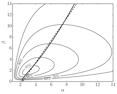
Figure 1: Map of geometry factor $G(\alpha,\beta)$, relative to its maximum value. The optimal value of $\alpha$ given a value of $\beta$ is shown by the diagonal solid line, and a linear fit of that line is shown by the dashed line.

Another important consideration is the maximum field a solenoid of given geometry is able to generate before surpassing the maximum allowable wire current density. Combining Eqs. 14 and 19 leads to an expression for the field strength given a wire current density $J$,

$$H_{\text{max}} =JR_{1}\beta\lambda\ln\left(\frac{\alpha+\sqrt{\alpha^{2}+\beta^{2}}}{1+\sqrt{1+\beta^{2}}}\right).$$ (24)

One should note that finding the optimal geometry for maximum field-per-power does not ensure that it is possible to reach a desired field strength without overstepping the maximum allowable wire current density. A departure from the optimal geometry may be necessary to reach the desired field strength with an acceptable current density. In other words, at the cost of more power per field strength, one may reach any desired field strength.

3.2 Thermomagnetic pumping

The performance of the thermomagnetic pump, in terms of the pressure increase achieved due to the magnetic force term (5), may be expressed as

$$\Delta p^{\text{mag}} =\int_{-\infty}^{\infty}f^{\text{mag}}\mathop{\mathrm{\mathstrut d}}\nolimits\!{x}$$

$$=\mu_{0}\int_{-\infty}^{\infty}M\frac{\partial H}{\partial x}\mathop{\mathrm{\mathstrut d}}\nolimits\!{x}.$$ (25)

In the following, it will be useful to note that the integral (25) is given by the area inside the parametric curve $(M(x),H(x))$.

A first approximation of the pump performance may be found by assuming that most of the temperature change from the left (upstream) $T_{\text{L}}$ to the right (downstream) $T_{\text{R}}$ happens within the centre of a solenoid, where the field is approximately constant and equal to $H_{\text{max}}$. In this case, Eq. 25 reduces to

$$\Delta p^{\text{mag}}=\mu_{0}\int_{0}^{H_{\text{max}}}\big{[}M(H,T_{\text{L}})\\ -M(H,T_{\text{R}})\big{]}\mathop{\mathrm{\mathstrut d}}\nolimits\!{H},$$ (26)

which is simply the area between the magnetization curves $M(H)$ at $T_{\text{L}}$ and $T_{\text{R}}$ up to $H_{\text{max}}$. This fact will be used in the discussion of the next section.

A second approximation may be found in the linear magnetization regime, where the magnetic field is weak and/or the temperature is high. Here one may assume that the susceptibility only depends on the temperature, that is, $\chi\equiv\chi(T)$. Thus, from Eqs. 26 and 6, we get

$$\Delta p^{\text{mag}} =\mu_{0}\int_{0}^{H_{\text{max}}}\left[\chi(T_{\text{L}})-\chi(T_{\text{R}})\right]H\mathop{\mathrm{\mathstrut d}}\nolimits\!{H}$$

$$=\frac{\mu_{0}}{2}\Delta\chi H_{\text{max}}^{2},$$ (27)

where $\Delta\chi\equiv\chi(T_{\text{L}})-\chi(T_{\text{R}})$, i.e. the change in magnetic susceptibility across the solenoid from left (upstream) to right (downstream). Again we remark that the integral is given by the area inside the $H$–$M$ curve, in this case as a triangle with vertices $(0,0)$, $(H_{\text{max}},M_{\text{L}})$ and $(H_{\text{max}},M_{\text{R}})$.

If we combine Eqs. 20 and 27, we can express the pumping performance only in terms of power consumption, solenoid properties, and change in ferrofluid susceptibility,

$$\Delta p^{\text{mag}}=\frac{\mu_{0}}{2}\Delta\chi\frac{\lambda G^{2}}{R_{1}\varrho}P.$$ (28)

3.3 Ferrofluid design

In the following, we will estimate a particle size distribution that gives an optimal thermomagnetic pumping effect for a given particle material, magnetic field and temperature range. We also provide some general design remarks and give an estimate for the pumping effect for a given case.

First, we note that the susceptibility of a ferrofluid with a particle volume fraction $\alpha_{\mathrm{p}}$ is given by

$$\chi=\alpha_{\mathrm{p}}\chi_{\mathrm{p}}=\alpha_{\mathrm{p}}\frac{M_{\mathrm{p}}(H,T)}{H},$$ (29)

where $M_{\mathrm{p}}$ is the average particle magnetization.

In [1], we present two different models for $M_{\mathrm{p}}$: The first assumes a uniform particle distribution (monodisperse), whereas the second uses a Gaussian particle distribution. The monodisperse model is used here, as it requires less computational work at the expense of accuracy. The model may be summarized as

$$M_{\mathrm{p}}(V_{\mathrm{p}},H,T)\\ =M_{\text{sat}}(T)\mathcal{L}\left(\frac{\mu_{0}V_{\mathrm{p}}M_{\text{sat}}(T)H}{k_{B}T}\right),$$ (30)

where $V_{\mathrm{p}}$ (${\mathrm{m}}^{3}\text{/}$) is the volume of a single particle, $\mathcal{L}$ is the Langevin function, and the saturation magnetization $M_{\text{sat}}(T)$ is modeled linearly to reach zero beyond a given Curie temperature, see [1]. Note that the Langevin function is approximately linear for small values of its argument. In this limit, the monodisperse model (30) reduces to what is called the Curie regime or Curie law.

Given a particle material, represented by the function $M_{\text{sat}}(T)$, a maximum field $H_{\text{max}}$ and a temperature range $T_{\text{L}}$ to $T_{\text{R}}$, we may use the particle magnetization model (30) to optimize the thermomagnetic pumping performance $\Delta p^{\text{mag}}$ as a function of particle size through Eq. 26. Here the particle concentration is only a factor between $M_{\mathrm{p}}$ and $M$, and so it does not affect the optimal particle size. It may thus be adjusted as desired after optimization.

From the optimization through Eq. 26, we find that the optimal particle size decreases with increasing $H_{\text{max}}$ and increases with increasing $T_{\text{R}}-T_{\text{L}}$. Further, we find that the magnetisation curves given an optimal particle size are such that $H_{\text{max}}$ is well beyond the Curie regime, with a magnetisation about $90\text{\,}\mathrm{\char 37\relax}\text{/}$ of saturation. This means that, for $T_{\text{L}}<T<T_{\text{R}}$,

$$M_{\mathrm{p}}(V_{p}^{\text{optim}},H_{\text{max}},T)\simeq 0.9M_{\text{sat}}(T).$$ (31)

An example of such an optimization may be seen in Fig. 2. Notice how $\Delta p^{\text{mag}}$ varies little for particle sizes that are close to the optimum. This means that there is considerable leeway for deviating from the optimum, for practical reasons such as stability. In particular, we find that increasing the particle size will not decrease performance much. However, decreasing the particle size will eventually lead to a rapid decrease in $\Delta p^{\text{mag}}$.

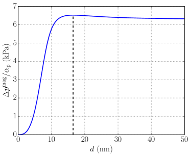
Figure 2: The estimated thermomagnetic pumping performance as a function of particle size, as given by Eq. 26. The particle volume fraction $\alpha_{\mathrm{p}}$ does not affect the optimization, and one may thus multiply with any chosed value to obtain the final $\Delta p^{\text{mag}}$. The particle material is the same as the one chosen in the main case study, and the optimization was performed for $H_{\text{max}}=$100\text{\,}\mathrm{kA}\text{/}\mathrm{m}$$, $T_{\text{L}}=$10\text{\,}\mathrm{\SIUnitSymbolCelsius}\text{/}$$ and $T_{\text{R}}=$50\text{\,}\mathrm{\SIUnitSymbolCelsius}\text{/}$$. The dashed line marks the identified optimum.

Provided that this optimization is performed, obtaining a large $\Delta p^{\text{mag}}$ then depends on:

• Having particles with a large saturation magnetization and a low Curie temperature.

• Having a large $\alpha_{\mathrm{p}}$, which may be limited by stability or viscosity concerns.

Aside from ferrofluid properties, the mechanisms giving efficient thermomagnetic pumping are then

• Increasing temperature from left to right, which will decrease both $1/T$ and $M_{\text{sat}}$ from left to right.

• Decreasing $\alpha_{\mathrm{p}}$ from left to right. This may be achieved by a decrease in the base fluid density, which through the conservation of base fluid mass flow will cause an increase in the velocity. An increase in the velocity will cause a decrease in $\alpha_{\mathrm{p}}$, through the conservation of particle mass flow. In single-phase flow, this may be caused by the slight thermal expansion of the liquid, but this effect mainly becomes significant when boiling occurs, which will drastically reduce the base fluid density.

Finally, it is of interest to estimate the magnitude of the thermomagnetic pumping force under optimal conditions. We use the approximation from Eq. 27. The largest possible value is obtained when the susceptibility $\chi$ on the downstream side of the solenoid vanishes, in which case $\Delta\chi$ is simply equal to $\chi$ on the upstream side. As noted above, the magnetization is about $90\text{\,}\mathrm{\char 37\relax}\text{/}$ of saturation at $H_{\text{max}}$. Thus, given some realistic values, $H_{\text{max}}=$100\text{\,}\mathrm{kA}\text{/}\mathrm{m}$$, $M_{\text{sat}}(T_{\text{L}})=$200\text{\,}\mathrm{kA}\text{/}\mathrm{m}$$ and $\alpha_{\mathrm{p}}=0.1$, we get an estimate for the pumping force, $\Delta p^{\text{mag}}\sim$1\text{\,}\mathrm{kPa}\text{/}$$.

4 Case specification

This section describes the setup of the case-study. The case is chosen such as to demonstrate the feasibility of enhancing a simple natural-convection based passive cooling concept by adding magnetic nanoparticles and a static magnetic field.

The case consists of a flow loop that connects a heat source to a heat sink, where a solenoid is placed over the heat source, see Fig. 3. At the lower left corner, we specify an initial pressure $p_{\mathrm{in}}=$1.0\text{\,}\mathrm{a}\mathrm{t}\mathrm{m}$$. The case may be thought of as the cooling of a hot device inside a larger object, with some cold reservoir, e.g. ocean water, available on the outside. We call these elements the heater and the cooler, respectively.

Note that the case is symmetric, and so will the natural convection and magnetic forces be if the fluid state is uniform around the loop. However, this equilibrium is unstable, and any beginning flow in one direction will induce stronger flow in the same direction. Exactly how to initiate this symmetry break is not the focus of this study, thus a counterclockwise flow is assumed.

Figure 3: A schematic of the simulated flow loop, showing the heat source at the bottom part and the heat sink at the top part. The solenoid cross-section is shown as hatched boxes. Gravity points downward in-plane. All dimensions are to scale. Arrows show chosen flow direction.

In the following, we describe in detail how the different parts of the case are modeled and defined. First, in Sec. 4.1 we describe the flow loop and the friction models. Next, in Sec. 4.2, we describe how the heater and cooler are modeled. In Sec. 4.3, we explain how the solenoid is designed by use of the previously discussed design rules. And finally, in Sec. 4.4 we describe the ferrofluid. In particular, we use the earlier results to get optimal nanoparticle sizes for the current case.

4.1 Flow loop

The flow loop is modeled as a simple pipe with diameter $D=$0.5\text{\,}\mathrm{c}\mathrm{m}$$, except at the heater and cooler where it is modeled as a bundle of ten smaller pipes of the same total flow cross section. The intruduction of tube bundles increases the fluid-to-wall heat transfer area, resulting in more heat transferred to the fluid and larger thermomagnetic and natural convection driving forces, at the expense of increased friction. The bundles are set to cover a cross section two times as large as the flow cross section, to make room for any (not currently modeled) heat exchanger cross flow. This increases the total pipe radius at the bundles by a factor of $\sqrt{2}$, which becomes the restriction on the inner radius of the solenoid.

The flow throughout the loop is mostly laminar, although some regions may have turbulent flow. We therefore use a friction factor model that depends on the local Reynolds number. For low Reynolds numbers, below 2100, we use a simple laminar model as described in [1]. For large Reynolds numbers, above 4000, we use the correlation by Haaland [20]. In the transition regime, that is for Reynolds numbers in the range 2100–4000, we use a smooth interpolation between the laminar and the turbulent friction models.

We remark that the Reynolds number will be approximately a constant multiplied with the local tube diameter along the flow loop, thus lower inside the heater/cooler than through the main loop. This follows because the total flow cross-section is constant throughout the rig, and so the mass flux is constant. Further, the ferrofluid viscosity is mostly constant, since the base fluid viscosity is constant.

4.2 Heater and cooler

For simplicity, the inner wall temperatures at the heater and cooler are kept constant. Herein lies an implicit assumption of no thermal resistance between the walls and external constant-temperature reservoirs.

The local heat transfer coefficients (HTCs) are calculated from the difference between the wall temperature and the local average fluid temperature. The particular HTC model or correlation that we use depends locally on the fluid, its state, and the temperature difference.

If there is no boiling or condensation, either at the heater or the cooler, the choice of HTC model depends on whether there are particles in the fluid or not. In the former case, the laminar Nusselt number correlation developed by Xuan and Li [21], shown in [4, Eq. 6], is used. In the latter case, the perfectly laminar Nusselt number of 3.66 is used. If there is boiling in the heater, sub-cooled or saturated, the correlation of Chen [22] is used. Sub-cooled boiling is initiated once the heater temperature is above the bubble temperature at the local pressure. For condensation at the cooler, the correlation by Boyko and Kruzhilin [23] is used. For boiling and condensation, the same correlations are used whether there are particles present or not. However, in the latter case, the ferroliquid properties are used instead of the pure liquid properties as input to the correlations.

4.3 Solenoid

In order to achieve an optimal thermomagnetic pumping force, we need as high a temperature difference between the peaks of $\mathop{\mathrm{\mathstrut d}}\nolimits\!{H}/\mathop{\mathrm{\mathstrut d}}\nolimits\!{x}$ as possible. Due to the fact that the thermomagnetic pump drives flow from a cold inlet to a hot outlet, it will only work if the field is at the heater, not the cooler. The solenoid must thus be placed around the heater. We use a solenoid length of $7.5\text{\,}\mathrm{cm}\text{/}$ so that it fully covers the heater.

As explained in Sec. 3.1, given a length, the optimal field per power is achieved when the inner radius is as small as possible. This means wrapping it around the heater bundle of a diameter which is $\sqrt{2}$ times the main pipe diameter, i.e. $0.71\text{\,}\mathrm{cm}\text{/}$. Using Eq. 23, the outer diameter should then be $5.38\text{\,}\mathrm{cm}\text{/}$. This corresponds to $\alpha=7.60$ and $\beta=10.6$, which as seen in Fig. 1 gives about $70\text{\,}\mathrm{\char 37\relax}\text{/}$ efficiency with respect to the field strength that would have been obtained if the the solenoid length were a free parameter. The resulting solenoid geometry is illustrated to scale in Fig. 3.

According to Eq. 24, this solenoid may reach fields of approximately $100\text{\,}\mathrm{kA}\text{/}\mathrm{m}$ before surpassing the allowed wire current density, and therefore the cases will be run with fields only up to this value.

4.4 Ferrofluid

The ferrofluid that we consider here is a mixture of a commercial ferrofluid (“TS50K”) and $n$-Hexane. This is similar to the ferrofluid that was used in the experiments by Iwamoto et al. [11], as well as in the validation of our model [1].

In Secs. 4.4.1 and 4.4.2, respectively, we describe in detail how the base fluid and particle properties are set. The properties are listed and summarized in Tab. 1.

Table 1: List of ferrofluid properties divided into model parameters and derived properties. (*): Standard ambient temperature and pressure ($300\text{\,}\mathrm{K}\text{/}$, $1\text{\,}\mathrm{a}\mathrm{t}\mathrm{m}$), where no vapor is present.

Description		Value
Model parameters
Base fluid
Mol. frac. decane	$z_{1}$	0.5
Mol. frac. hexane	$z_{2}$	0.5
Liquid viscosity	$\eta_{\mathrm{\ell}}$	$5.31\text{\times}{10}^{-4}\text{\,}\mathrm{Pa}\text{\,}\mathrm{s}\text{/}$
Vapor viscosity	$\eta_{\mathrm{v}}$	$7.65\text{\times}{10}^{-6}\text{\,}\mathrm{Pa}\text{\,}\mathrm{s}\text{/}$
Liquid conductivity	$\lambda_{\mathrm{\ell}}$	$0.130\text{\,}\mathrm{W}\text{/}\text{(}\mathrm{m}\text{\,}\mathrm{K}\text{)}$
Vapor conductivity	$\lambda_{\mathrm{v}}$	$0.0202\text{\,}\mathrm{W}\text{/}\text{(}\mathrm{m}\text{\,}\mathrm{K}\text{)}$
Surface tension	$\sigma_{\mathrm{bf}}$	$0.0120\text{\,}\mathrm{N}\text{/}\mathrm{m}$
Nanoparticles
Density	$\rho_{\mathrm{p}}$	$5000\text{\,}\mathrm{kg}\text{/}{\mathrm{m}}^{3}$
Specific heat capacity	$c_{\mathrm{p}}^{p}$	$750\text{\,}\mathrm{J}\text{/}\text{(}\mathrm{kg}\text{\,}\mathrm{K}\text{)}$
Sat. mag. at $300\text{\,}\mathrm{\SIUnitSymbolCelsius}\text{/}$	$M_{\text{sat}}^{\circ}$	$250.0\text{\,}\mathrm{kA}\text{/}\mathrm{m}$
Curie temperature	$T_{\text{C}}$	$500\text{\,}\mathrm{K}\text{/}$
Conductivity	$\lambda_{\mathrm{p}}$	$29.0\text{\,}\mathrm{W}\text{/}\text{(}\mathrm{m}\text{\,}\mathrm{K}\text{)}$
Particle diameter	$d_{\mathrm{p}}$	$10.0\text{\,}\mathrm{nm}\text{/}$
Inlet volume fraction	$\alpha_{\mathrm{p},{\mathrm{in}}}$	$10\text{\,}\mathrm{\char 37\relax}\text{/}$
Derived properties
Base fluid
Density (*)		$700.2\text{\,}\mathrm{kg}\text{/}{\mathrm{m}}^{3}$
Heat. cap. (*)		$2252\text{\,}\mathrm{J}\text{/}\text{(}\mathrm{kg}\text{\,}\mathrm{K}\text{)}$
Vol. heat. cap. (*)		$1576\text{\,}\mathrm{kJ}\text{/}\text{(}{\mathrm{m}}^{3}\text{\,}\mathrm{K}\text{)}$
Bubble point ($1\text{\,}\mathrm{a}\mathrm{t}\mathrm{m}$)		$91.6\text{\,}\mathrm{\SIUnitSymbolCelsius}\text{/}$
Latent heat ($1\text{\,}\mathrm{a}\mathrm{t}\mathrm{m}$)		$320.4\text{\,}\mathrm{kJ}\text{/}\mathrm{kg}$
Ferroliquid ($\alpha_{\mathrm{p}}=0.1$)
Density (*)		$1130\text{\,}\mathrm{kg}\text{/}{\mathrm{m}}^{3}$
Heat. cap. (*)		$1626\text{\,}\mathrm{J}\text{/}\text{(}\mathrm{kg}\text{\,}\mathrm{K}\text{)}$
Vol. heat. cap. (*)		$1837\text{\,}\mathrm{kJ}\text{/}\text{(}{\mathrm{m}}^{3}\text{\,}\mathrm{K}\text{)}$
Viscosity		$6.91\text{\times}{10}^{-4}\text{\,}\mathrm{Pa}\text{\,}\mathrm{s}\text{/}$
Conductivity		$0.173\text{\,}\mathrm{W}\text{/}\text{(}\mathrm{m}\text{\,}\mathrm{K}\text{)}$

4.4.1 Base fluid

The base fluid of TS50K is kerosene, which is a mixture of more than 20 components. As in [1], we use undecane to represent the kerosene so that the base fluid of the ferrofluid is a binary hydrocarbon mixture of hexane and decane. The hexane and decane were mixed in equal molar amounts, which corresponds to $62\text{\,}\mathrm{\char 37\relax}\text{/}$ decane and $38\text{\,}\mathrm{\char 37\relax}\text{/}$ hexane on a mass basis. We note that the hexane is more volatile than the decane.

For a given temperature and pressure, the thermodynamic properties of the mixture, such as density, heat capacity, enthalpy, latent heat and liquid–vapor equilibrium, are predicted from the thermodynamic equation of state based on these components and their relative amounts. This process is described in [1].

We used data from [24] for the transport properties of the components. The liquid properties were taken at $1\text{\,}\mathrm{a}\mathrm{t}\mathrm{m}$ and $20\text{\,}\mathrm{\SIUnitSymbolCelsius}\text{/}$, while the vapor properties were taken at the component boiling point at $1\text{\,}\mathrm{a}\mathrm{t}\mathrm{m}$. The transport properties of the components were combined into base fluid mixture properties for each phase based on the overall composition fractions. For the mixture viscosity, we used the Grunberg and Nissan equation [25], and for the mixture conductivity, we used the Filippov equation [26]. The mixture surface tension was calculated as a simple molar fraction weighted average of the two components.

The viscosity and conductivity of the ferroliquid phase (liquid phase and particles) is a modification of the base liquid properties according to correlations stated in [1]. The surface tension is assumed unmodified by the presence of nanoparticles.

4.4.2 Particles

The ferrofluid is made of MnZn-Ferrite particles. Exact values for the density and heat capacity are difficult to know precisely, as they will depend on the relative amounts of Mn and Zn. The values will also be different in nanoparticle form compared to bulk values. Reasonable values close to the ones used in [1] were chosen. The value for thermal conductivity was taken from [27].

The material magnetization properties $M_{\text{sat}}^{\circ}$ and $T_{\text{C}}$ were set in the reasonable region found when fitting to experimental MnZn-Ferrite ferrofluid magnetization data [1].

The remaining particle property is the diameter. An optimization as described in Sec. 3.3 was performed, and an optimum was found at about $16\text{\,}\mathrm{nm}\text{/}$, as seen in Fig. 2. However, all sizes above $10\text{\,}\mathrm{nm}\text{/}$ showed $\Delta p^{\text{mag}}$ values above about $90\text{\,}\mathrm{\char 37\relax}\text{/}$ of the optimum, and were thus considered good candidates. To avoid stability concerns, and because it is a common particle size for ferrofluids, a size of $10\text{\,}\mathrm{nm}\text{/}$ was chosen for this study. The magnetization curves resulting from these parameters may be seen in Fig. 4.

The achievable $\Delta\chi$, and thus also the potential performance of the thermomagnetic pump, is expected to scale with the particle volume fraction. However, to ensure the practical relevance of the results obtained, the inlet volume fraction $\alpha_{\mathrm{p},{\mathrm{in}}}$ is kept at a moderate $10\text{\,}\mathrm{\char 37\relax}\text{/}$, which is in the range of common commercial ferrofluids.

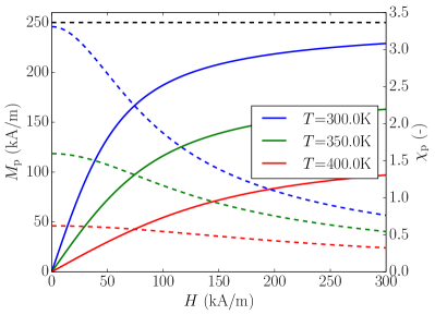
Figure 4: The magnetization curves (solid lines, left axis) and susceptibilities (dashed lines, right axis) of the particle ensemble, given the parameters in Tab. 1, at different temperatures. The horizontal dashed line marks the saturation magnetization at $300\text{\,}\mathrm{K}\text{/}$.

5 Results

We use the procedure and model equations described in Sec. 2 to obtain steady periodic solutions for the case described in the previous section. The results from the simulations are presented here and will be further discussed in the next section.

Two variables were varied:

• $\Delta T$: The temperature difference between the heater and cooler, which is changed by changing the heater temperature. The cooler was kept at $T_{\text{cold}}=$10\text{\,}\mathrm{\SIUnitSymbolCelsius}\text{/}$$, to simulate heat exchange against seawater.

• $H_{\text{max}}$: The maximum field strength provided by the solenoid, which relates to the solenoid power dissipation according to Eq. 20.

Since the flow loop is vertical, a driving force from natural convection will always be present. This effect alone serves as a reference for the following results. The reference case was run across the range of $\Delta T$, with no particles and no field, giving conventional natural convection with a conventional fluid.

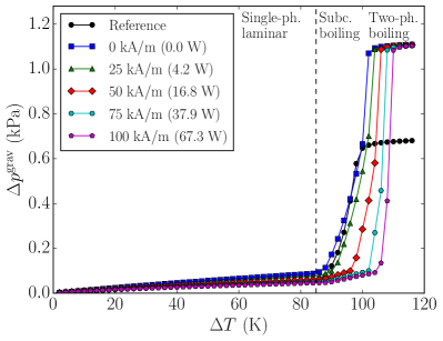
Figure 5: The pressure contribution from natural convection calculated from simulation results through Eq. 32, for varying $\Delta T$ and $H_{\text{max}}$.

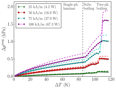
Figure 6: The pressure contribution from the thermomagnetic pump calculated from simulation results through Eq. 33, for varying $\Delta T$ and $H_{\text{max}}$. Above each line is a dashed line showing the approximation found by using Eq. 27, where only $\Delta\chi$ is taken from the simulation results.

Generally, there are two driving forces for the flow: the thermomagnetic pump and the natural convection. Each may be quantified by their net contribution to the pressure-change around the loop. We may define the pressure contributions as

$$\Delta p^{\text{grav}}=\oint f^{\text{grav}}\mathop{\mathrm{\mathstrut d}}\nolimits\!{x},$$ (32)

and

$$\Delta p^{\text{mag}}=\oint f^{\text{mag}}\mathop{\mathrm{\mathstrut d}}\nolimits\!{x},$$ (33)

where the gravitational and magnetic force terms are described in [1] and Eq. 5, respectively.

The integration is performed around the whole loop in the counterclockwise flow direction. Of course, the solution demands that the total $\Delta p$ around the whole loop is zero. The cancelling contribution is the friction force.

The validity of the estimate (27) may be tested by comparing it to Eq. 33 as calculated from a simulation. The $\Delta\chi$ to insert in (27) is then calculated by evaluating Eq. 29 at the left and right end of the solenoid from the simulation results.

The calculated values for $\Delta p^{\text{grav}}$ and $\Delta p^{\text{mag}}$ for varying $\Delta T$ and $H_{\text{max}}$ are presented in Figs. 5 and 6, respectively. The estimates from Eq. 27 are included in Fig. 6 for comparison.

The total rate of heat transported from the heater to the cooler, denoted as $Q$ ($\mathrm{W}\text{/}$), may be used as a performance metric for the whole case. The calculated values of $Q$ are shown in Fig. 7 for varying $\Delta T$ and $H_{\text{max}}$.

However, for a fair comparison with natural convection, the performance metric should take into account the power consumption of the solenoid $P$. The power consumption is dissipated as heat and adds to the total amount of heat to be transported away by the fluid. The effective heat that is transported from the heat source is therefore $Q_{\text{eff}}$ ($\mathrm{W}\text{/}$),

$$Q_{\text{eff}}\equiv Q-P.$$ (34)

For the comparison, we calculate the relative improvement or the enhancement factor, that is $Q_{\text{eff}}/Q_{\text{ref}}$, where $Q_{\text{ref}}$ is the reference result with no particles, that is, pure natural convection. The effective enhancement is presented in Fig. 8.

Fig. 9 shows the pressure and temperature along the rig at the point of maximum enhancement, i.e. at about $\Delta T=$80\text{\,}\mathrm{K}\text{/}$$. At this same point, we also investigated the sensitivity in the nanofluid heat transfer correlation (HTC). Tab. 2 shows the results where the HTC is adjusted with $\pm$20\text{\,}\mathrm{\char 37\relax}\text{/}$$.

Finally, Fig. 10 shows the Reynolds number in front of the heater and at the center of the heater as a function of temperature differences, and for varying magnetic fields.

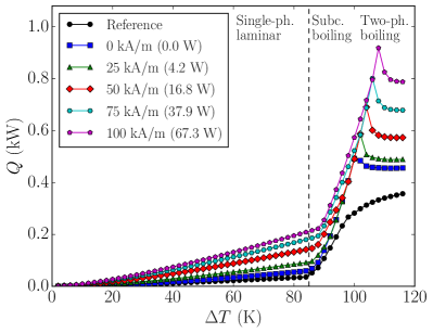
Figure 7: Total rate of heat transfer between heater and cooler, for varying $\Delta T$ and $H_{\text{max}}$, and for the reference case with no particles and no field.

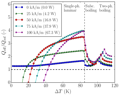
Figure 8: The effective enhancement of cooling power, relative to the reference case with no particles and no field, for varying $\Delta T$ and $H_{\text{max}}$. The horizontal dashed line shows the limit where the increased heat transfer rate is just enough to remove the additional heat added by the solenoid.

Table 2: Effects on total heat transfer $Q$ ($\mathrm{W}\text{/}$) by $\pm$20\text{\,}\mathrm{\char 37\relax}\text{/}$$ in the nanofluid heat transfer correlation for the $\Delta T=$80\text{\,}\mathrm{K}\text{/}$$ case. Percentages are relative to the first row.

	$H=$0\text{\,}\mathrm{kA}\text{/}\mathrm{m}$$		$H=$100\text{\,}\mathrm{kA}\text{/}\mathrm{m}$$
Orig.	54.7		195.1
$+$20\text{\,}\mathrm{\char 37\relax}\text{/}$$	60.7	($+$11\text{\,}\mathrm{\char 37\relax}\text{/}$$)	235.5	($+$21\text{\,}\mathrm{\char 37\relax}\text{/}$$)
$-$20\text{\,}\mathrm{\char 37\relax}\text{/}$$	47.2	($-$14\text{\,}\mathrm{\char 37\relax}\text{/}$$)	153.4	($-$21\text{\,}\mathrm{\char 37\relax}\text{/}$$)

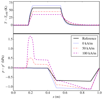
Figure 9: The pressure (bottom), relative to pressure at $x=0$, and temperature (top), relative to cooler temperature, plotted against position $x$ along the rig for a set of cases with $\Delta T=$80\text{\,}\mathrm{K}\text{/}$$. The magnetization symmetry breaking can be seen as the pressure jump between $x=0.1$ and $x=0.3$, which is approximately equal to $\Delta p_{\text{mag}}$. If there was no symmetry breaking, then there would be no pressure difference here.

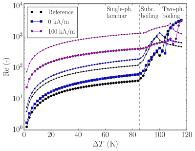
Figure 10: The Reynolds number as a function of temperature difference, as measured before the heater (small markers) and at the center of the heater (large markers).

6 Discussion

6.1 Driving forces

The two driving forces for flow, in terms of their contribution to pressure increase around the loop, were shown in Figs. 5 and 6. This section will explain and discuss their features as the two main variables are changed.

The natural convection is driven by a difference in fluid density at the right and left ends of the loop. The density difference is caused by thermal expansion of the liquid due to temperature differences, as well as the presence of vapor on the right side in the boiling cases.

On both ends of the solenoid, the magnetic force points in towards the solenoid center. The key to the thermomagnetic pumping effect is the magnetization symmetry breaking, which is to reduce the downstream magnetic force compared to the upstream one, and thus achieve a positive $\Delta p^{\text{mag}}$, as seen in Fig. 9. The thermomagnetic pumping is therefore driven by a decrease of susceptibility $\chi$ across the heater (see Eq. 27), and as mentioned in Sec. 3.3, there are two mechanisms for this. First, an increase in fluid temperature decreases the susceptibility of the particle phase, as shown in Fig. 4. Second, a decrease in base fluid density increases the flow velocity, and thus decreases the concentration of particles $\alpha_{\mathrm{p}}$ by “stretching” the particle distribution. The effect of the thermomagnetic pump may also be seen in Fig. 10, which shows that the Reynolds number increases when the magnetic field is increased.

The results, presented in Figs. 5 and 6, reveal three distinct regimes: A single-phase regime, a transition regime with sub-cooled boiling, and a two-phase regime. Below approximately $\Delta T=$85\text{\,}\mathrm{K}\text{/}$$, the heater temperature is below the local bubble temperatures. Here there is no vapor, nor or any kind of boiling heat transfer. Still, increasing $\Delta T$ increases the fluid temperature differences, and thus both driving forces increase. Note that in this regime, $\Delta p^{\text{mag}}$ dominates over $\Delta p^{\text{grav}}$ at the higher field strengths, and thus the thermomagnetic pumping is the major driving force.

At higher $\Delta T$, in the transition regime, sub-cooled boiling is active at the heater. This means that the heater temperature is above the bubble temperature, but the average base fluid state is still in the liquid region. In this regime, local boiling at the walls increase the heat transfer coefficient at the heater. This increase leads to a rapid enhancement of both driving forces.

In the two-phase regime where the fluid temperature after the heater has passed the bubble temperature, we enter the saturated boiling heat transfer regime. While the vapor fraction on the right vertical section increases due to boiling, $\Delta p^{\text{grav}}$ increases rapidly with $\Delta T$, as seen in Fig. 5. The driving force eventually reaches a final plateau where most of the hexane is vaporized, in which case there is no more density difference to be gained. The height of this plateau is independent of the magnetic field, since it does not affect the liquid-vapor density difference. However, it does depend on the presence of particles, as they affect the mass of the ferroliquid phase.

As seen in Fig. 6, the thermomagnetic pumping force also sees a rapid increase as two-phase flow starts to occur. This is due to the sudden decrease in $\alpha_{\mathrm{p}}$ compared to the heater inlet, which decreases $\chi_{\text{R}}$, and thus increases $\Delta\chi$. This driving force also reaches an optimal plateau as the vapor fraction reaches its plateau. On this plateau, the symmetry breaking of the magnetization response is near its optimum, as $\chi_{\text{R}}\ll\chi_{\text{L}}$. The pressure jump $\Delta p^{\text{mag}}$ is then approximately given by Eq. 27 with $\chi_{\text{L}}$ substituted in place of $\Delta\chi$. We also remark here that the simple calculation of the pumping force given at the end of Sec. 3, that is, $\Delta p^{\text{mag}}\sim$1\text{\,}\mathrm{kPa}\text{/}$$ for $H_{\text{max}}=$100\text{\,}\mathrm{kA}\text{/}\mathrm{m}$$, gives a coarse but reasonable estimate.

As opposed to the plateau of $\Delta p^{\text{grav}}$, the plateau of $\Delta p^{\text{mag}}$ depends on $H_{\text{max}}$. From Eq. 27 we see that it increases as the square of $H_{\text{max}}$, or by considering Eq. 20, linearly with solenoid power consumption. Note that the plateau of $\Delta p^{\text{mag}}$ at the highest field strength is about $50\text{\,}\mathrm{\char 37\relax}\text{/}$ greater than the plateau of $\Delta p^{\text{grav}}$. This shows that the thermomagnetic force can be the major driving force also in the boiling regime.

From Fig. 6, we see that Eq. 27 gives a reasonable but slightly high estimate for $\Delta p^{\text{mag}}$. Given a magnetization model and a field strength, Eq. 27 provides $\Delta p^{\text{mag}}$ as an explicit function of $T$ and $\alpha_{\mathrm{p}}$ at the heater inlet and outlet, which could prove very useful for more high-level engineering of complex systems. If one wants an even simpler relation, one can assume that $\chi_{\text{R}}\ll\chi_{\text{L}}$ and thus $\Delta\chi=\chi_{\text{L}}$. This gives a best-case estimate, which only depends on $\chi=\alpha_{\mathrm{p}}\chi_{\mathrm{p}}$ at the inlet. This corresponds to the final plateaus in Fig. 6.

From Fig. 5, we see that $\Delta p^{\text{grav}}$ is reduced with increasing magnetic field in the single-phase regime, and the appearance of vapor is pushed to higher $\Delta T$. This is due to the added $\Delta p^{\text{mag}}$ increasing the flow velocity, which suppresses temperature change when passing the heater and cooler. However, the added $\Delta p^{\text{mag}}$ ensures a net increase in total driving force.

6.2 Cooling performance enhancements

The three regimes discussed in the previous section can also be identified in the total heat transfer rate $Q$, as seen in Fig. 7. Before the onset of boiling, it increases smoothly with $\Delta T$. It also increases when particles are added, and further with the magnetic field. As boiling initiates, an abrupt increase is seen in a transition phase, before it stabilizes on plateaus in the saturated boiling regime.

As mentioned, it is important to account for the heat added by the solenoid. A more fair performance measure is therefore $Q_{\text{eff}}$, which may be interpreted as the maximum power the cooled device may be run at while still keeping it at the target temperature. The enhancements of this, relative to the reference case, are seen in Fig. 8.

When entering the boiling regime at the heater, $Q$ increases rapidly for all cases. However, we see a sudden drop in $Q_{\text{eff}}$, which is due to the fact that the reference case increases more rapidly. Simply put, entering boiling heat transfer is a much greater leap from conventional laminar heat transfer than from nanofluid-enhanced laminar heat transfer. When entering saturated boiling and two-phase flow, there is a transition to turbulent friction in some regions, leading to a decrease in $Q$ in some cases, but eventually we see a stabilization.

The performance enhancement in a given case can come from two different effects. First, there is the nanofluid effect, which is the effect of the fluid having different intrinsic properties compared to if no particles were present. Second, there is the thermomagnetic pumping effect, which is the effect of adding the magnetic field, which introduces the $\Delta p^{\text{mag}}$ driving force that was discussed in the previous section.

The most likely $\Delta T$-areas of operation are either the laminar pure single-phase (no boiling) regime or well into the saturated boiling regime. Tab. 3 lists the best possible enhancements in cooling performance in these regimes, with the particle amount and field strengths considered here.

Table 3: The best performance enhancement factors found compared to the reference case, in the single-phase (ferroliquid) and two-phase/boiling (ferroliquid+vapor) regimes, from the nanofluid effect and the thermomagnetic pumping effect. The first column shows the enhancement seen from the addition of nanoparticles alone, while the second column shows the additional enhancement seen from thermomagnetic pumping. The third column shows the total enhancement with thermomagnetic pumping compared to the reference.

	Nanofluid	Thermomagnetic	Total
1-phase	1.7	2.4	4.0
2-phase	1.3	1.5	2.0

Note that these results depend on the quite conservatively chosen particle volume fraction of $10\text{\,}\mathrm{\char 37\relax}\text{/}$. Higher amounts are possible, and since both enhancement effects scale with $\alpha_{\mathrm{p}}$, higher enhancements could also be possible. This would be a trade-off between performance and stability/viscosity concerns.

6.2.1 Nanofluid effect

As seen in Fig. 8 and Tab. 3, performance enhancements in the area of $50\text{\,}\mathrm{\char 37\relax}\text{/}$ are within reach, simply by adding nanoparticles to the base fluid.

We studied which effects in the model that contributed to these performance enhancements by turning them off one by one, and observed how $Q$ in the new solution differs from the original. We found that the nanofluid enhancement comes from increases in Nusselt number, conductivity, and volumetric heat capacity (see Tab. 1). The relative amounts of each depend on the heat transfer regime.

6.2.2 Thermomagnetic pumping effect

As seen in Fig. 7, $Q$ always increases when the magnetic field strength increases. However, when subtracting the solenoid power dissipation, Fig. 8 reveals that different $H_{\text{max}}$ are optimal depending on $\Delta T$. As seen in Fig. 8 and Tab. 3, the thermomagnetic pumping effect can provide significant enhancements on top of the nanofluid effect, in both the single-phase and two-phase boiling regimes. The most significant enhancements are seen in the single-phase regime, even though one sees from Fig. 9 that the symmetry breaking is far from complete, and much less than in the two-phase boiling cases. However, in these cases, there are only weak laminar friction forces, and therefore there is much flow velocity to be gained from $\Delta p^{\text{mag}}$.

At very low $\Delta T$, the magnetic symmetry breaking, i.e. $\Delta\chi$, is so small that the net thermomagnetic pumping cannot compensate for the heat dissipated from the solenoid. When a curve is below the dashed line in Fig. 8, it is better to turn the solenoid off. The magnetic forces may still be large, but on each side of the solenoid they point inwards with almost equal strength, giving very little net force.

6.2.3 Permanent magnets

Although the thermomagnetic concept described here is passive with respect to the lack of moving parts, it may still be argued that the thermomagnetic solution is not truly passive, since the solenoid requires power input. However, it is worth noting that the magnetic field strengths used in this study are well within the range of what is possible with permanent magnets. Using permanent magnets instead of a solenoid will eliminate the solenoid power consumption and heat dissipation. This would reduce power consumption to zero, give higher effective enhancements, and make it a truly passive concept like natural convection.

As there are no longer any free currents involved, Maxwell’s equations demand that

$$\int_{-\infty}^{\infty}H(x)\mathop{\mathrm{\mathstrut d}}\nolimits\!{x}=0,$$ (35)

along the central axis, which prohibits the simple $H(x)\geq 0$ field-profile possible with a solenoid. However, even though the $H(x)$ profile from a configuration of permanent magnets must have a higher number of extrema, both positive and negative, there is no reason why one cannot obtain a similar symmetry breaking and net pumping effect.

6.3 Compactness

The benefits may also be viewed in terms of compactness of the cooling system, instead of increased performance given the same size.

One dimension of compactness is the rig height (originally $10\text{\,}\mathrm{cm}\text{/}$), which is a required component of the natural convection effect. Adding the nanofluid- and thermomagnetic effect may allow for the reduction of height while retaining a performance no less than the reference case. In the $H_{\text{max}}=$100\text{\,}\mathrm{kA}\text{/}\mathrm{m}$$ case, we see from Figs. 5 and 6 that $\Delta p^{\text{mag}}$ is larger than $\Delta p^{\text{grav}}$ in both regimes, which indicates that one could make the rig completely flat while still retaining some enhancement compared to the reference. Additional simulations with no gravity were run to investigate this. In the single-phase regime, almost all the enhancement remained, since $\Delta p^{\text{mag}}$ is so dominant. In the two-phase boiling regime, an enhancement of 1.5X remained.

Another dimension of compactness is the length of the heat sink (originally $30\text{\,}\mathrm{cm}\text{/}$), which may be reduced when adding the nanofluid- and thermomagnetic effect. It turns out that in both regimes, the heat sink length may be reduced to about $25\text{\,}\mathrm{\char 37\relax}\text{/}$ of its original size, while retaining the original performance.

6.4 Concept limitations

While the enhancements found seem promising, it is worth noting that the nature of the concept puts some restrictions on where it can be used:

• Since the pumping force will be from the cold side to the hot side of the field source, the field source must be placed at the heat source of the loop, not the heat sink. Otherwise, the flow will be damped instead of enhanced.

• The magnetic field source should stretch across the heat source from end to end, to achieve as high a fluid temperature difference as possible between the ends. The aspect ratio of the heat source must then allow for a solenoid with a reasonable field-per-power efficiency, as shown in Fig. 1. However, designs using permanent magnets will make the field-per-power concern irrelevant.

• While we have accounted for the heat dissipation of the solenoid through the need for additional heat removal, that does not mean that the additional needed electrical energy input is desired. However, permanent magnets may also alleviate this, as discussed in Sec. 6.2.3.

Note that the above limitations are for the thermomagnetic pumping effect, and that the nanofluid effect should be more widely applicable.

6.5 Comments on model limitations

As in any model, some simplifications are made which could affect the results. In this section, we will discuss the most relevant of these, and how they may or may not add uncertainty to the conclusions.

First, regarding the heat transfer coefficients, one could argue that assuming $\text{Nu}=3.66$ when the reference fluid is single-phase is a low estimate, as the flow would not immediately become well developed. This is quantified by the Graetz number, $\text{Gz}(x^{\prime})=D\text{Re}\text{Pr}/x^{\prime}$, where $D$ ($\mathrm{m}\text{/}$) is the tube diameter and $x^{\prime}$ ($\mathrm{m}\text{/}$) is the distance from the heater/cooler inlet. It is commonly cited that the flow is well developed from the point where Gr drops below $20$. We will here consider the single-phase cases with the highest Re, $\Delta T=$80\text{\,}\mathrm{K}\text{/}$$. In the reference case, we see $\text{Re}\approx 40$ in the bundles (cf. Fig. 10), and $\text{Gz}<20$ is satisfied about $40\text{\,}\mathrm{\char 37\relax}\text{/}$ into the heater. This means it is mostly well developed, but we underestime the average Nu to some degree. In the $H=$100\text{\,}\mathrm{kA}\text{/}\mathrm{m}$$ ferrofluid case, we see $\text{Re}\approx 400$ in the bundles and $\text{Gr}\approx 80$ at the heater outlet. This means that the flow does not have time to fully develop. As the Xuan–Li correlation is presumably also for developed laminar flow, we will here also underestimate the actual Nu. However, we will underestimate the nanofluid Nu to a greater degree, and we therefore argue that the found enhancements from the nanofluid effect, Tab. 3, are conservative.

Second, there is some evidence that the classical model may underpredict the nanofluid viscosity enhancement [28]. If this is so, the actual enhancement from the nanofluid effect would be lower than the one reported here.

However, neither of the above points can disturb the additional enhancements predicted from the thermomagnetic pumping effect. The introduction of thermomagnetic pumping may however introduce an additional viscosity increase, called the magnetoviscous effect [29]. This effect is not present in the model, but we argue that it will be negligible under the conditions of the cases studied here. First, even in the noninteracting dipole regime, there may be rotational magnetoviscosity. However, the flow in the heater bundle is in the regime where it is negligible, according to [30]. Second, interactions between particles may give additional effects, but it turns out that these particles at these temperatures are in the weakly interacting regime, as defined in [29], where thermal energy prevents magnetic chaining/clustering. Here the viscosity increase appear to be around $10\text{\,}\mathrm{\char 37\relax}\text{/}$ at worst, and less in the linear magnetization regime. In any case, magnetoviscosity is only present at the solenoid, which is a small part of the loop as a whole, and thus contributes relatively little to the total friction.

As concluded in the experimental validation of this model [1], the thermomagnetic pumping is very sensitive to the temperature change across the solenoid, and thus to the HTC model used. Tab. 2 shows the sensitivity of the total heat transfer to variations in the HTC at $\Delta T=$80\text{\,}\mathrm{K}$$ for the reference case $H=$0\text{\,}\mathrm{k}\mathrm{A}\mathrm{/}\mathrm{m}$$ and for $H=$100\text{\,}\mathrm{k}\mathrm{A}\mathrm{/}\mathrm{m}$$. The table shows that the relative uncertainty in total heat transfer is of the same order of magnitude as the relative uncertainty in HTC.

7 Conclusions and further work

For the simplified cooling system studied here, we may conclude that:

• The thermomagnetic driving force is significant compared to natural convection, and in the single-phase case it can be several times larger.

• Using a ferrofluid can provide significant performance enhancements for the cooling system:

  • The nanofluid effect alone can improve performance by a factor 1.7 in the single-phase laminar cases, and 1.3 in the two-phase boiling cases.

  • Adding the thermomagnetic effect with a solenoid can give an additional performance enhancement of 2.4 (4.0 total) in the single-phase laminar cases, and 1.5 (2.0 total) in the two-phase boiling cases, even when taking into account the additional heat from ohmic losses in the solenoid.

• Using a ferrofluid can provide significant compactness while retaining original (or better) cooling performance:

  • The thermomagnetic effect can completely replace the natural convection driving force, while still retaining a cooling performance enhancement of $50\text{\,}\mathrm{\char 37\relax}\text{/}$ or more. This eliminates the required rig height, enabling more compact solutions.

  • Using a ferrofluid can allow reductions of heat sink size to about $25\text{\,}\mathrm{\char 37\relax}\text{/}$ of original size while retaining original performance.

Additionally, we have:

• Derived design rules for optimal field-per-power solenoid, as shown in Sec. 3.1.2.

• Derived design rules for optimal ferrofluid for thermomagnetic pumping, as shown in Sec. 3.3.

• Derived and validated a reasonably accurate approximation for the thermomagnetic pumping performance, shown in Eq. 27 and Eq. 28, which may be useful for higher level engineering considerations.

Note that the performance enhancements found are specific to this case study, and may vary with size scales and variations in rig design. However, this study does demonstrate a great practical potential for using thermomagnetically pumped ferrofluids to enhance heat transfer systems. Further studies should explore the range of applicability.

The possibility of using permanent magnets in place of solenoids, as mentioned in Sec. 6.2.3, is very interesting for applications where additional power consumption is inconvenient. Similar studies could explore this using the same model, only using a $H(x)$ calculated from a configuration of permanent magnets.

References

- Aursand et al. [2016] E. Aursand, M. Aa. Gjennestad, K. Y. Lervåg, H. Lund, A multi-phase ferrofluid flow model with equation of state for thermomagnetic pumping and heat transfer, Journal of Magnetism and Magnetic Materials 402 (2016) 8–19, doi:10.1016/j.jmmm.2015.11.042.
- Taylor et al. [2013] R. Taylor, S. Coulombe, T. Otanicar, P. Phelan, A. Gunawan, W. Lv, G. Rosengarten, R. Prasher, H. Tyagi, Small particles, big impacts: A review of the diverse applications of nanofluids, Journal of Applied Physics 113 (2013) 011301, doi:10.1063/1.4754271.
- Choi and Eastman [1995] S. Choi, J. Eastman, Enhancing thermal conductivity of fluids with nanoparticles, URL http://www.osti.gov/scitech/servlets/purl/196525, 1995.
- Kakaç and Pramuanjaroenkij [2009] S. Kakaç, A. Pramuanjaroenkij, Review of convective heat transfer enhancement with nanofluids, International Journal of Heat and Mass Transfer 52 (13) (2009) 3187–3196, doi:10.1016/j.ijheatmasstransfer.2009.02.006.
- Xuan and Li [2000] Y. Xuan, Q. Li, Heat transfer enhancement of nanofluids, International Journal of Heat and Fluid Flow 21 (1) (2000) 58–64, doi:10.1016/S0142-727X(99)00067-3.
- Maiga et al. [2005] S. E. B. Maiga, S. J. Palm, C. T. Nguyen, G. Roy, N. Galanis, Heat transfer enhancement by using nanofluids in forced convection flows, International Journal of Heat and Fluid Flow 26 (4) (2005) 530–546, doi:10.1016/j.ijheatfluidflow.2005.02.004.
- Odenbach [2003] S. Odenbach, Ferrofluids—magnetically controlled suspensions, Colloids and Surfaces A: Physicochemical and Engineering Aspects 217 (2003) 171–178, doi:10.1016/S0927-7757(02)00573-3.
- Rosensweig [1985] R. E. Rosensweig, Ferrohydrodynamics, Cambridge University Press, Cambridge, ISBN 0486678342, 1985.
- Lian et al. [2009a] W. Lian, Y. Xuan, Q. Li, Characterization of miniature automatic energy transport devices based on the thermomagnetic effect, Energy Conversion and Management 50 (1) (2009a) 35–42, doi:10.1016/j.enconman.2008.09.005.
- Xuan and Lian [2011] Y. Xuan, W. Lian, Electronic cooling using an automatic energy transport device based on the thermomagnetic effect, Applied Thermal Engineering 31 (2011) 1487–1494, doi:10.1016/j.applthermaleng.2011.01.033.
- Iwamoto et al. [2011] Y. Iwamoto, H. Yamaguchi, X.-D. Niu, Magnetically-driven heat transport device using a binary temperature-sensitive magnetic fluid, Journal of Magnetism and Magnetic Materials 323 (2011) 1378–1383, doi:10.1016/j.jmmm.2010.11.050.
- Yamaguchi and Iwamoto [2013] H. Yamaguchi, H. Iwamoto, Heat transport with temperature-sensitive magnetic fluid for application to micro-cooling device, Magnetohydrodynamics 49 (3–4) (2013) 448–453.
- Iwamoto et al. [2012] Y. Iwamoto, X.-D. Niu, H. Yamaguchi, H. Yamasaki, T. Kuwahara, Magnetically-Driven Heat Transport Device using Ferrofluid, Journal of JSEM 12 (Special Issue) (2012) 99–104, doi:10.11395/jjsem.12.s99.
- Karimi-Moghaddam et al. [2014] G. Karimi-Moghaddam, R. D. Gould, S. Bhattacharya, A non-dimensional analysis to characterize thermomagnetic convection of a temperature sensitive magnetic fluid in a flow loop, Journal of Heat Transfer 136 (9) (2014) 091702, doi:10.1115/1.4027863.
- Lian et al. [2009b] W. Lian, Y. Xuan, Q. Li, Design method of automatic energy transport devices based on thermodynamic effect of magnetic fluids, International Journal of Heat and Mass Transfer 52 (2009b) 5451–5458, doi:10.1016/j.ijheatmasstransfer.2009.06.031.
- Michelsen and Mollerup [2007] M. L. Michelsen, J. M. Mollerup, Thermodynamic Models: Fundamentals & computational aspects, Tie-Line Publications, Holte, Denmark, second edn., ISBN 8798996134, 2007.
- Jones et al. [01 ] E. Jones, T. Oliphant, P. Peterson, et al., SciPy: Open source scientific tools for Python, URL http://www.scipy.org/, 2001–.
- Moré et al. [1980] J. J. Moré, B. S. Garbow, K. E. Hillstrom, User Guide for MINPACK-1, Tech. Rep. ANL-80-74, Argonne National Laboratory, Argonne, IL, USA, 1980.
- Jiles [1998] D. Jiles, Introduction to Magnetism and Magnetic Materials, Second Edition, Taylor & Francis, Boca Raton, ISBN 9780412798603, 1998.
- Haaland [1983] S. E. Haaland, Simple and explicit formulas for the friction factor in turbulent pipe flow, J. Fluids Eng. 105 (1983) 89–90, doi:10.1115/1.3240948.
- Xuan and Li [2003] Y. Xuan, Q. Li, Investigation on convective heat transfer and flow features of nanofluids, Journal of Heat transfer 125 (1) (2003) 151–155, doi:10.1115/1.1532008.
- Chen [1966] J. C. Chen, Correlation for boiling heat transfer to saturated fluids in convective flow, Industrial & Engineering Chemistry Process Design and Development 5 (3) (1966) 322–329, doi:10.1021/i260019a023.
- Boyko and Kruzhilin [1967] L. D. Boyko, G. N. Kruzhilin, Heat transfer and hydraulic resistance during condensation of steam in a horizontal tube and in a bundle of tubes, International Journal of Heat and Mass Transfer 10 (3) (1967) 361–373, doi:10.1016/0017-9310(67)90152-4.
- NIS [2014] NIST Chemistry WebBook, NIST Standard Reference Database Number 69, http://webbook.nist.gov, (retrieved November 4, 2014).
- Grunberg and Nissan [1949] L. Grunberg, A. H. Nissan, Mixture law for viscosity, Nature 164 (1949) 799–800, doi:10.1038/164799b0.
- Filippov [1968] L. P. Filippov, Liquid thermal conductivity research at Moscow University, International Journal of Heat and Mass Transfer 11 (2) (1968) 331–345, doi:10.1016/0017-9310(68)90161-0.
- Lee [2000] E.-S. Lee, Surface characteristics in the precision grinding of Mn-Zn ferrite with in-process electro-discharge dressing, Journal of Materials Processing Technology 104 (3) (2000) 215 – 225, doi:10.1016/S0924-0136(00)00562-8.
- Rudyak [2013] V. Y. Rudyak, Viscosity of nanofluids. Why it is not described by the classical theories, Advances in Nanoparticles 2 (03) (2013) 266, doi:10.4236/anp.2013.23037.
- Ilg and Odenbach [2009] P. Ilg, S. Odenbach, Ferrofluid structure and rheology, in: Colloidal Magnetic Fluids, vol. 763 of Lecture Notes in Physics, Springer, 249–325, doi:10.1007/978-3-540-85387-9_4, 2009.
- Rosensweig et al. [1969] R. E. Rosensweig, R. Kaiser, G. Miskolczy, Viscosity of magnetic fluid in a magnetic field, Journal of Colloid and Interface Science 29 (4) (1969) 680–686, doi:10.1016/0021-9797(69)90220-3.