An algebraic description of screw dislocations in SC and BCC crystal lattices

Abstract.

We give an algebraic description of screw dislocations in a crystal, especially simple cubic (SC) and body centered cubic (BCC) crystals, using free abelian groups and fibering structures. We also show that the strain energy of a screw dislocation based on the spring model is expressed by the Epstein-Hurwitz zeta function approximately.

1. Introduction

Mathematical descriptions of dislocations in crystal lattices have been studied extensively in the framework of differential geometry or continuum geometry [A1, A2, KE, Kon, N]. However, crystal structures are usually given as discrete geometry. In fact, a crystal lattice is governed by a discrete group such as free abelian group [CS, Koh, S]. An abelian group and its group ring provide fruitful mathematical tools, e.g., abelian varieties, theta functions, and so on. On the other hand, the continuum geometric nature of dislocations in the euclidean space cannot be represented well as long as we use the ordinary algebraic expressions.

In this article, we give algebraic descriptions of screw dislocations in the simple cubic (SC) and the body centered cubic (BCC) crystals in terms of certain “fibrations” involving group rings. Using such fibering structures, we describe the continuum geometric property embedded in the euclidean space, whereas the algebraic structures involving group rings enable us to describe the discrete nature of the crystal lattices. More precisely, we first describe the screw dislocations in continuum picture and then we use algebraic structures of lattices to embed their “discrete dislocations” in the continuum description. Our key idea is to use certain sections of $S^{1}$-bundles to control the behavior of dislocations.

We also show that the strain energy of a screw dislocation based on the spring model is expressed by the Epstein-Hurwitz zeta function [Ep, El] approximately. This will be shown by using our algebraic description of a screw dislocation.

It should be noted that the results presented in this article arose in our attempt to solve the following problems proposed in the Study Group Workshop at Kyushu University and the University of Tokyo, held during July 29–Aug 4, 2015 [O].

1. To find a proper mathematical description of a screw dislocation in the BCC lattice.

2. To find a proper mathematical description of the strain energy of a screw dislocation in the BCC lattice.

The present article is organized as follows. In Section 2, we first introduce certain fibering structures over the plane involving the celebrated exact sequence

$$0\to{\mathbb{Z}}\to{\mathbb{R}}\to{\mathrm{U}}(1)\to 1,$$

which will be essential in this article. Then, we will describe screw dislocations in continuum picture, in which certain covering spaces of a punctured complex plane will play important roles. By using certain path spaces, we clarify the covering structures of screw dislocations in Remark 2.4 and Proposition 2.6. In Section 3, we first explain the algebraic structure of the SC lattice as a free abelian group. Then, we consider the fibering structure of the SC lattice in terms of the associated group ring and its quotient. Using these descriptions, we will describe the screw dislocations in the SC lattice in Propositions 3.6 and 3.8 so that they are embedded in the continuum picture given in Section 2. In Section 4, we first explain the fibering structure of the SC lattice in a diagonal direction, using group ring structures. Then, we explain similar structures for the BCC lattice. Finally, screw dislocations in the BCC lattice will be described using all these algebraic materials in Propositions 4.14 and 4.15. Section 5 is devoted to the computation of the strain or elastic energy of a single screw dislocation in the SC lattice. In Theorem 5.3, the elastic energy of the dislocation corresponding to a bounded annular region is expressed in terms of the truncated Epstein-Hurwitz zeta function [Ep, El] approximately. In Section 6, we give some remarks on our results from mathematical viewpoints. In Section 7, we explain and interpret our results in details from physical points of view so that even the readers who may not be familiar with mathematical tools can understand the novelty of our results. Finally, in the appendix, we show that the total elastic energy for a pair of parallel screw dislocations with opposite directions does not diverge for unbounded regions in the continuum picture, and we also show the convergence in the discrete picture for the principal part of the energy.

1.1. Notations and Conventions

Throughout the article, we distinguish the euclidean space ${\mathbb{E}}$ from the real vector space ${\mathbb{R}}$: in particular, ${\mathbb{R}}$ is endowed with an algebraic structure, while ${\mathbb{E}}$ is not. We often identify the $2$-dimensional euclidean space ${\mathbb{E}}^{2}$ with the complex plane ${\mathbb{C}}$. The group $U(1)$ acts on the set $S^{1}$ simply transitively. Given a fiber bundle ${\mathcal{F}}\rightarrow{\mathcal{M}}$ over a base space ${\mathcal{M}}$, we denote the set of all continuous sections $f:{\mathcal{M}}\to{\mathcal{F}}$ by $\Gamma({\mathcal{M}},{\mathcal{F}})$.

2. Screw Dislocations in Continuum Picture

Let us consider the exact sequence of groups (see [B])

(2.1)

where ${\mathbb{Z}}$ and ${\mathbb{R}}$ are additive groups, ${\mathrm{U}}(1)$ is a multiplicative group, $\iota(n)=n$ for $n\in{\mathbb{Z}}$, and $(\exp 2\pi{\sqrt{-1}})(x)=\exp(2\pi{\sqrt{-1}}x)$ for $x\in{\mathbb{R}}$. Throughout this section, we fix $d>0$. For $\delta\in{\mathbb{R}}$, we have the “shifts”

$$\widetilde{\iota}_{\delta}:{\mathbb{R}}\to{\mathbb{E}}\mbox{ defined by }x\mapsto d\cdot x+\delta,\,x\in{\mathbb{R}},\mbox{ and}$$

$$\iota_{\delta}:{\mathrm{U}}(1)\to S^{1}\mbox{ defined by }\exp({{\sqrt{-1}}\theta})\mapsto\exp{{\sqrt{-1}}(\theta+2\pi\delta/d)},\,\theta\in{\mathbb{R}},$$

such that the following diagram is commutative:

where $\psi(y)=\exp(2\pi{\sqrt{-1}}y/d)$, $y\in{\mathbb{R}}$, and $\varphi_{\delta}=\widetilde{\iota}_{\delta}\circ\iota$. Note that for the sequence of maps

we have

(2.2) $$\varphi_{\delta}({\mathbb{Z}})=\psi^{-1}(\exp(2\pi{\sqrt{-1}}\delta/d)),$$

which is a consequence of the exactness of (2.1).

2.1. Fibering Structures of Crystals in Continuum Picture

Let us consider the $2$-dimensional euclidean space ${\mathbb{E}}^{2}$ and some trivial bundles over ${\mathbb{E}}^{2}$; ${\mathbb{Z}}$-bundle $\pi_{{\mathbb{Z}}}:{\mathbb{Z}}_{{\mathbb{E}}^{2}}\to{\mathbb{E}}^{2}$, ${\mathbb{E}}$-bundle $\pi_{{\mathbb{E}}}:{\mathbb{E}}_{{\mathbb{E}}^{2}}\to{\mathbb{E}}^{2}$ and $S^{1}$-bundle $\pi_{S^{1}}:S^{1}_{{\mathbb{E}}^{2}}\to{\mathbb{E}}^{2}$. We consider the bundle maps $\widehat{\varphi}_{\delta}$ and $\widehat{\psi}$,

(2.3) $$\lx@xy@svg{\hbox{\raise 0.0pt\hbox{\kern 8.76111pt\hbox{\ignorespaces\ignorespaces\ignorespaces\hbox{\vtop{\kern 0.0pt\offinterlineskip\halign{\entry@#!@&&\entry@@#!@\cr&&\crcr}}}\ignorespaces{\hbox{\kern-8.76111pt\raise 0.0pt\hbox{\hbox{\kern 0.0pt\raise 0.0pt\hbox{\hbox{\kern 3.0pt\raise 0.0pt\hbox{$\textstyle{{\mathbb{Z}}_{{\mathbb{E}}^{2}}\ignorespaces\ignorespaces\ignorespaces\ignorespaces}$}}}}}}}\ignorespaces\ignorespaces\ignorespaces\ignorespaces{}{\hbox{\lx@xy@droprule}}\ignorespaces\ignorespaces\ignorespaces{\hbox{\kern 14.09444pt\raise 7.30556pt\hbox{{}\hbox{\kern 0.0pt\raise 0.0pt\hbox{\hbox{\kern 3.0pt\hbox{\hbox{\kern 0.0pt\raise-2.91667pt\hbox{$\scriptstyle{\widehat{\varphi}_{\delta}}$}}}\kern 3.0pt}}}}}}\ignorespaces{\hbox{\kern 32.76111pt\raise 0.0pt\hbox{\hbox{\kern 0.0pt\raise 0.0pt\hbox{\lx@xy@tip{1}\lx@xy@tip{-1}}}}}}{\hbox{\lx@xy@droprule}}{\hbox{\lx@xy@droprule}}{\hbox{\kern 32.76111pt\raise 0.0pt\hbox{\hbox{\kern 0.0pt\raise 0.0pt\hbox{\hbox{\kern 3.0pt\raise 0.0pt\hbox{$\textstyle{{\mathbb{E}}_{{\mathbb{E}}^{2}}\ignorespaces\ignorespaces\ignorespaces\ignorespaces}$}}}}}}}\ignorespaces\ignorespaces\ignorespaces\ignorespaces{}{\hbox{\lx@xy@droprule}}\ignorespaces\ignorespaces\ignorespaces{\hbox{\kern 57.2pt\raise 6.61111pt\hbox{{}\hbox{\kern 0.0pt\raise 0.0pt\hbox{\hbox{\kern 3.0pt\hbox{\hbox{\kern 0.0pt\raise-3.61111pt\hbox{$\scriptstyle{\widehat{\psi}}$}}}\kern 3.0pt}}}}}}\ignorespaces{\hbox{\kern 74.97778pt\raise 0.0pt\hbox{\hbox{\kern 0.0pt\raise 0.0pt\hbox{\lx@xy@tip{1}\lx@xy@tip{-1}}}}}}{\hbox{\lx@xy@droprule}}{\hbox{\lx@xy@droprule}}{\hbox{\kern 74.97778pt\raise 0.0pt\hbox{\hbox{\kern 0.0pt\raise 0.0pt\hbox{\hbox{\kern 3.0pt\raise 0.0pt\hbox{$\textstyle{S^{1}_{{\mathbb{E}}^{2}}}$}}}}}}}\ignorespaces}}}}\ignorespaces, \textstyle{{\mathbb{Z}}_{{\mathbb{E}}^{2}}\ignorespaces\ignorespaces\ignorespaces\ignorespaces} \scriptstyle{\widehat{\varphi}_{\delta}} \textstyle{{\mathbb{E}}_{{\mathbb{E}}^{2}}\ignorespaces\ignorespaces\ignorespaces\ignorespaces} \scriptstyle{\widehat{\psi}} \textstyle{S^{1}_{{\mathbb{E}}^{2}}} \textstyle{{\mathbb{Z}}_{{\mathbb{E}}^{2}}\ignorespaces\ignorespaces\ignorespaces\ignorespaces} \scriptstyle{\widehat{\varphi}_{\delta}} \textstyle{{\mathbb{E}}_{{\mathbb{E}}^{2}}\ignorespaces\ignorespaces\ignorespaces\ignorespaces} \scriptstyle{\widehat{\psi}} \textstyle{S^{1}_{{\mathbb{E}}^{2}}}$$

naturally induced by $\varphi_{\delta}$ and $\psi$, respectively.

Note that ${\mathbb{Z}}_{{\mathbb{E}}^{2}}={\mathbb{Z}}\times{\mathbb{E}}^{2}$ is a covering space of ${\mathbb{E}}^{2}$ and that ${\mathbb{E}}_{{\mathbb{E}}^{2}}$ is identified with ${\mathbb{E}}^{3}={\mathbb{E}}\times{\mathbb{E}}^{2}$. We sometimes use such identifications.

In the following, we often identify ${\mathbb{E}}^{2}$ with the complex plane ${\mathbb{C}}$. For $\gamma\in S^{1}$, let us consider the global constant section $\sigma_{\gamma}\in\Gamma({\mathbb{E}}^{2},S^{1}_{{\mathbb{E}}^{2}})$ of $S^{1}_{{\mathbb{E}}^{2}}$ defined by

$$\sigma_{\gamma}(z)=(\gamma,z)\in S^{1}_{{\mathbb{E}}^{2}}=S^{1}\times{\mathbb{E}}^{2}$$

for $z\in{\mathbb{E}}^{2}={\mathbb{C}}$. The following lemma is straightforward by virtue of (2.2).

Lemma 2.1.

For $\gamma=\exp(2\pi{\sqrt{-1}}\delta/d)$, we have

$${\mathbb{Z}}_{{\mathbb{E}}^{2},\gamma}=\widehat{\varphi}_{\delta}({\mathbb{Z}}_{{\mathbb{E}}^{2}}),$$

where

$${\mathbb{Z}}_{{\mathbb{E}}^{2},\gamma}:={\widehat{\psi}^{-1}}\left(\sigma_{\gamma}({\mathbb{E}}^{2})\right)\subset{\mathbb{E}}^{3}.$$

2.2. Single Screw Dislocation in Continuum Picture

For $z_{0}\in{\mathbb{E}}^{2}={\mathbb{C}}$, let us consider the trivial bundles ${\mathbb{E}}_{{\mathbb{E}}^{2}\setminus\{z_{0}\}}$ and $S^{1}_{{\mathbb{E}}^{2}\setminus\{z_{0}\}}$ over ${\mathbb{E}}^{2}\setminus\{z_{0}\}$ as in the previous subsection. For $\gamma\in S^{1}$, let us consider the section $\sigma_{z_{0},\gamma}\in\Gamma({\mathbb{E}}^{2}\setminus\{z_{0}\},S^{1}_{{\mathbb{E}}^{2}\setminus\{z_{0}\}})$ defined by

$$\sigma_{z_{0},\gamma}(z)=\left(\gamma\frac{z-z_{0}}{|z-z_{0}|},z\right)\mbox{ for }z\in{\mathbb{E}}^{2}\setminus\{z_{0}\}={\mathbb{C}}\setminus\{z_{0}\}.$$

We set

$${\mathbb{Z}}_{{\mathbb{E}}^{2}\setminus\{z_{0}\},\gamma}:={\widehat{\psi}^{-1}}\left(\sigma_{z_{0},\gamma}({\mathbb{E}}^{2}\setminus\{z_{0}\})\right)\subset{\mathbb{E}}_{{\mathbb{E}}^{2}\setminus\{z_{0}\}}\subset{\mathbb{E}}^{3}$$

and let $\pi_{z_{0},\gamma}:{\mathbb{Z}}_{{\mathbb{E}}^{2}\setminus\{z_{0}\},\gamma}\to{\mathbb{E}}^{2}\setminus\{z_{0}\}$ be defined by $\pi_{z_{0},\gamma}=\pi_{{\mathbb{E}}}|{{\mathbb{Z}}_{{\mathbb{E}}^{2}\setminus\{z_{0}\},\gamma}}$.

Lemma 2.2.

The map $\pi_{z_{0},\gamma}:{\mathbb{Z}}_{{\mathbb{E}}^{2}\setminus\{z_{0}\},\gamma}\to{\mathbb{E}}^{2}\setminus\{z_{0}\}$ defines a universal covering of ${\mathbb{E}}^{2}\setminus\{z_{0}\}$.

Proof.

Over each point of ${\mathbb{E}}^{2}$, $\widehat{\psi}$ is a covering map and it is trivial as a family of covering maps. Therefore, we see that $\pi_{z_{0},\gamma}$ defines a covering map.

Furthermore, ${\mathbb{Z}}_{{\mathbb{E}}^{2}\setminus\{z_{0}\},\gamma}$ is path-wise connected. This is seen as follows. Let us take arbitrary two points $x_{1}$ and $x_{2}$. Then $\pi_{z_{0},\gamma}(x_{1})$ and $\pi_{z_{0},\gamma}(x_{2})$ are connected by a path in ${\mathbb{E}}^{2}\setminus\{z_{0}\}$. By lifting such a path, we see that $x_{1}$ is connected in ${\mathbb{Z}}_{{\mathbb{E}}^{2}\setminus\{z_{0}\},\gamma}$ to a point $x_{1}^{\prime}$ such that $\pi_{z_{0},\gamma}(x_{1}^{\prime})=\pi_{z_{0},\gamma}(x_{2})$, which we denote by $\bar{x}$. Then, by lifting a loop based at $\bar{x}$ which turns around $z_{0}$ for an appropriate number of times, we see that $x_{1}^{\prime}$ is connected to $x_{2}$ in ${\mathbb{Z}}_{{\mathbb{E}}^{2}\setminus\{z_{0}\},\gamma}$. Therefore, ${\mathbb{Z}}_{{\mathbb{E}}^{2}\setminus\{z_{0}\},\gamma}$ is path-wise connected.

Moreover, the lift of a loop $\ell$ in ${\mathbb{E}}^{2}\setminus\{z_{0}\}$ by $\pi_{z_{0},\gamma}$ is a loop if and only if its winding number around $z_{0}$ vanishes. This is because the section $\sigma_{z_{0},\gamma}$ over $\ell$ winds around $S^{1}$ by the same number of times as it winds around $z_{0}$. This implies that the action of $\pi_{1}({\mathbb{E}}^{2}\setminus\{z_{0}\})$ on ${\mathbb{Z}}_{{\mathbb{E}}^{2}\setminus\{z_{0}\},\gamma}$ is effective. Therefore, $\pi_{z_{0},\gamma}$ is a universal covering. This completes the proof. ∎

Remark 2.3.

It should be noted that ${\mathbb{Z}}_{{\mathbb{E}}^{2}\setminus\{z_{0}\},\gamma}$ is embedded in ${\mathbb{E}}_{{\mathbb{E}}^{2}\setminus\{z_{0}\}}\subset{\mathbb{E}}^{3}$. This represents a screw dislocation in a crystal in continuum picture. The point $z_{0}$ corresponds to the position of the dislocation line.

Remark 2.4.

A standard universal covering space ${\mathbb{Z}}_{{\mathbb{E}}^{2}\setminus\{z_{0}\}}$ of ${\mathbb{E}}^{2}\setminus\{z_{0}\}$ is constructed as follows. Fixing a point $x_{0}\in{\mathbb{E}}^{2}\setminus\{z_{0}\}$, we consider the path space (see [BT])

$${\mathrm{Path}}({\mathbb{E}}^{2}\setminus\{z_{0}\}):=\{\mbox{continuous maps }\mu:[0,1]\to{\mathbb{E}}^{2}\setminus\{z_{0}\}\,|\,\mu(0)=x_{0}\}/\sim,$$

where two paths $\mu$ and $\nu$ are equivalent, written as $\mu\sim\nu$, if $\mu(1)=\nu(1)$ and $\mu$ is homotopic to $\nu$ relative to end points in ${\mathbb{E}}^{2}\setminus\{z_{0}\}$. The path space is the quotient space with respect to the equivalence, where it is endowed with the natural topology induced from that of the locally simply connected space ${\mathbb{E}}^{2}\setminus\{z_{0}\}$. Then the map $\pi_{\mathrm{Path}}:{\mathrm{Path}}({\mathbb{E}}^{2}\setminus\{z_{0}\})\ni\mu\mapsto\mu(1)\in{\mathbb{E}}^{2}\setminus\{z_{0}\}$ defines a universal covering. Note that $\pi_{\mathrm{Path}}^{-1}(z)$, $z\in{\mathbb{E}}^{2}\setminus\{z_{0}\}$, is regarded as the set of winding numbers around $z_{0}$, i.e. $\pi_{\mathrm{Path}}^{-1}(z)={\mathbb{Z}}$ up to a shift. Then, we define

$${\mathbb{Z}}_{{\mathbb{E}}^{2}\setminus\{z_{0}\}}:={\mathrm{Path}}({\mathbb{E}}^{2}\setminus\{z_{0}\}).$$

It should be noted that the space obtained does not depend on the choice of the point $x_{0}$, up to a covering equivalence.

By virtue of Lemma 2.2 together with the uniqueness of the universal covering, we can construct an embedding $\widehat{\varphi}_{z_{0},\delta}:{\mathbb{Z}}_{{\mathbb{E}}^{2}\setminus\{z_{0}\}}\to{\mathbb{E}}_{{\mathbb{E}}^{2}\setminus\{z_{0}\}}$ such that the diagram

commutes and

$$\widehat{\varphi}_{z_{0},\delta}({\mathbb{Z}}_{{\mathbb{E}}^{2}\setminus\{z_{0}\}})={\mathbb{Z}}_{{\mathbb{E}}^{2}\setminus\{z_{0}\},\gamma}\subset{\mathbb{E}}^{3}$$

holds for $\gamma=\exp(2\pi{\sqrt{-1}}\delta/d)$. In other words, we have the sequence

(2.4)

as a non-trivial analogue of (2.3) in such a way that $\widehat{\psi}\circ\widehat{\varphi}_{z_{0},\delta}({\mathbb{Z}}_{{\mathbb{E}}^{2}\setminus\{z_{0}\}})=\sigma_{z_{0},\gamma}({\mathbb{E}}^{2}\setminus\{z_{0}\})$ and that $\widehat{\varphi}_{z_{0},\delta}({\mathbb{Z}}_{{\mathbb{E}}^{2}\setminus\{z_{0}\}})$ represents a single screw dislocation in a crystal.

2.3. Multi-Screw Dislocation in Continuum Picture

Let us now consider multiple screw dislocations that are parallel to each other. They are described as follows.

Let ${\mathcal{S}}={\mathcal{S}}_{+}\coprod{\mathcal{S}}_{-}$ be a finite subset of ${\mathbb{E}}^{2}$, which is divided into disjoint subsets ${\mathcal{S}}_{+}$ and ${\mathcal{S}}_{-}$. Let us consider the trivial bundles ${\mathbb{E}}_{{\mathbb{E}}^{2}\setminus{\mathcal{S}}}$ and $S^{1}_{{\mathbb{E}}^{2}\setminus{\mathcal{S}}}$ over ${\mathbb{E}}^{2}\setminus{\mathcal{S}}$ as in the previous subsections. Then, we consider the section $\sigma_{{\mathcal{S}},\gamma}\in\Gamma({\mathbb{E}}^{2}\setminus{\mathcal{S}},S^{1}_{{\mathbb{E}}^{2}\setminus{\mathcal{S}}})$ defined by

(2.5) $$\sigma_{{\mathcal{S}},\gamma}(z)=\left(\gamma\prod_{z_{i}\in{\mathcal{S}}_{+}}\frac{z-z_{i}}{|z-z_{i}|}\cdot\prod_{z_{j}\in{\mathcal{S}}_{-}}\frac{\overline{z-z_{j}}}{|z-z_{j}|},z\right)\mbox{ \rm for }z\in{\mathbb{E}}^{2}\setminus{\mathcal{S}}={\mathbb{C}}\setminus{\mathcal{S}},$$

where $\overline{z-z_{j}}$ is the complex conjugate of $z-z_{j}$. We enumerate the points in ${\mathcal{S}}$ in such a way that

$${\mathcal{S}}_{+}=\{z_{1},z_{2},\ldots,z_{s}\},\quad{\mathcal{S}}_{-}=\{z_{s+1},z_{s+2},\ldots,z_{s+t}\},$$

where $n=s+t$ is the cardinality of ${\mathcal{S}}$.

Definition 2.5.

Set

$${\mathbb{Z}}_{{\mathbb{E}}^{2}\setminus{\mathcal{S}},\gamma}:={\widehat{\psi}^{-1}}\left(\sigma_{{\mathcal{S}},\gamma}({\mathbb{E}}^{2}\setminus{\mathcal{S}})\right)\subset{\mathbb{E}}^{3}\setminus\pi_{{\mathbb{E}}}^{-1}({\mathcal{S}})\subset{\mathbb{E}}^{3}$$

and define $\pi_{{\mathcal{S}},\gamma}:{\mathbb{Z}}_{{\mathbb{E}}^{2}\setminus{\mathcal{S}},\gamma}\to{\mathbb{E}}^{2}\setminus{\mathcal{S}}$ by $\pi_{{\mathcal{S}},\gamma}=\pi_{{\mathbb{E}}}|{{\mathbb{Z}}_{{\mathbb{E}}^{2}\setminus{\mathcal{S}},\gamma}}$.

As in Lemma 2.2, we see that $\pi_{{\mathcal{S}},\gamma}$ defines a covering map. Note also that the covering space ${\mathbb{Z}}_{{\mathbb{E}}^{2}\setminus{\mathcal{S}},\gamma}$ of ${\mathbb{E}}^{2}\setminus{\mathcal{S}}$ is realized in ${\mathbb{E}}^{3}$. This represents multiple parallel screw dislocations in a crystal in continuum picture. The set ${\mathcal{S}}$ corresponds to the positions of the dislocation lines.

Now, let us clarify the nature of the covering $\pi_{{\mathcal{S}},\gamma}:{\mathbb{Z}}_{{\mathbb{E}}^{2}\setminus{\mathcal{S}},\gamma}\to{\mathbb{E}}^{2}\setminus{\mathcal{S}}$. As in Remark 2.4, we can define the path space

$${\mathrm{Path}}({\mathbb{E}}^{2}\setminus{\mathcal{S}}):=\{\mbox{continuous maps }\mu:[0,1]\to{\mathbb{E}}^{2}\setminus{\mathcal{S}}\,|\,\mu(0)=x_{0}\}/\sim,$$

using the same equivalence relation, where we fix a point $x_{0}\in{\mathbb{E}}^{2}\setminus{\mathcal{S}}$. This is the universal covering space of ${\mathbb{E}}^{2}\setminus{\mathcal{S}}$. However, for our purpose, this space is too big, and we need to take certain quotients.

Note that the fundamental group $G=\pi_{1}({\mathbb{E}}^{2}\setminus{\mathcal{S}},x_{0})$ is a free group of rank $n$ generated by $m_{1},m_{2},\ldots,m_{n}$, where $m_{i}$ is the element of $G$ represented by a loop based at $x_{0}$ which turns around $z_{i}$ once in the counterclockwise direction and which does not turn around $z_{j}$, $j\neq i$. Let $G^{\prime}=[G,G]$ be the commutator subgroup of $G$. By taking the orbit space under the natural action of $G^{\prime}$, we get the universal abelian covering space of ${\mathbb{E}}\setminus{\mathcal{S}}$, denoted by ${\mathrm{Path}}^{a}({\mathbb{E}}^{2}\setminus{\mathcal{S}})$. In other words, we have

$${\mathrm{Path}}^{a}({\mathbb{E}}^{2}\setminus{\mathcal{S}}):=\{\mbox{continuous maps }\mu:[0,1]\to{\mathbb{E}}^{2}\setminus{\mathcal{S}}\,|\,\mu(0)=x_{0}\}/\sim_{a},$$

where for two paths $\mu$ and $\nu$, we have $\mu\sim_{a}\nu$ if $\mu(1)=\nu(1)$ and the loop $\mu\ast\overline{\nu}$ based at $x_{0}$ represents an element of $G^{\prime}$, where $\mu\ast\overline{\nu}$ denotes the product path of $\mu$ and the inverse path of $\nu$.

Note that the homology group $H_{1}({\mathbb{E}}^{2}\setminus{\mathcal{S}};{\mathbb{Z}})$ is isomorphic to ${\mathbb{Z}}^{n}$, which is freely generated by the homology classes $[m_{1}],[m_{2}],\ldots,[m_{n}]$ represented by $m_{1},m_{2},\ldots,m_{n}$, respectively. Note also that $H_{1}({\mathbb{E}}^{2}\setminus{\mathcal{S}};{\mathbb{Z}})$ is isomorphic to the quotient group $G/G^{\prime}$. An arbitrary element $\kappa$ of $H_{1}({\mathbb{E}}^{2}\setminus{\mathcal{S}};{\mathbb{Z}})$ is represented as $\sum_{i}w_{i}[m_{i}]$, where $w_{i}\in{\mathbb{Z}}$ is the winding number of $\kappa$ around $z_{i}$ in the direction of $m_{i}$. Therefore, for a loop $\ell$ in ${\mathbb{E}}^{2}\setminus{\mathcal{S}}$, its lift in ${\mathrm{Path}}^{a}({\mathbb{E}}^{2}\setminus{\mathcal{S}})$ is a loop if and only if the winding number of $\ell$ around each point of ${\mathcal{S}}$ vanishes.

Let us now define

$${\mathbb{Z}}^{n}_{{\mathbb{E}}^{2}\setminus{\mathcal{S}}}:={\mathrm{Path}}^{a}({\mathbb{E}}^{2}\setminus{\mathcal{S}}),\quad\pi_{{\mathrm{Path}}^{a}}:{\mathbb{Z}}^{n}_{{\mathbb{E}}^{2}\setminus{\mathcal{S}}}\to{\mathbb{E}}^{2}\setminus{\mathcal{S}},$$

where $\pi_{{\mathrm{Path}}^{a}}$ sends the class of each path to its terminal point. Note that $\pi_{{\mathrm{Path}}^{a}}$ defines a covering, and that for each $z\in{\mathbb{E}}^{2}\setminus{\mathcal{S}}$, $\pi_{{\mathrm{Path}}^{a}}^{-1}(z)$ can be identified with ${\mathbb{Z}}^{n}$ up to a certain “shift”.

Let us now take further quotients. Let $h:\pi_{1}({\mathbb{E}}^{2}\setminus{\mathcal{S}},x_{0})\to{\mathbb{Z}}$ be the homomorphism defined by

$$h(m_{i})=\left\{\begin{array}[]{lr}1,&1\leq i\leq s,\\ -1,&s+1\leq i\leq s+t.\end{array}\right.$$

Since ${\mathbb{Z}}$ is abelian, the kernel $H$ of $h$ contains $G^{\prime}$. Let ${\mathbb{Z}}_{{\mathbb{E}}^{2}\setminus{\mathcal{S}}}$ be the orbit space of ${\mathrm{Path}}({\mathbb{E}}^{2}\setminus{\mathcal{S}})$ under the natural action of $H$. In other words, we have

$${\mathbb{Z}}_{{\mathbb{E}}^{2}\setminus{\mathcal{S}}}:=\{\mbox{continuous maps }\mu:[0,1]\to{\mathbb{E}}^{2}\setminus{\mathcal{S}}\,|\,\mu(0)=x_{0}\}/\sim_{h},$$

where for two paths $\mu$ and $\nu$, we have $\mu\sim_{h}\nu$ if $\mu(1)=\nu(1)$ and the loop $\mu\ast\overline{\nu}$ based at $x_{0}$ represents an element of $H$. We have a natural projection $\pi_{H}:{\mathbb{Z}}_{{\mathbb{E}}^{2}\setminus{\mathcal{S}}}\to{\mathbb{E}}^{2}\setminus{\mathcal{S}}$ which sends the class of each path to its terminal point. Note that $\pi_{H}$ defines a covering map.

Proposition 2.6.

The coverings $\pi_{{\mathcal{S}},\gamma}:{\mathbb{Z}}_{{\mathbb{E}}^{2}\setminus{\mathcal{S}},\gamma}\to{\mathbb{E}}^{2}\setminus{\mathcal{S}}$ and $\pi_{H}:{\mathbb{Z}}_{{\mathbb{E}}^{2}\setminus{\mathcal{S}}}\to{\mathbb{E}}^{2}\setminus{\mathcal{S}}$ are equivalent.

Proof.

Fix a point $\tilde{x}_{0}\in{\mathbb{Z}}_{{\mathbb{E}}^{2}\setminus{\mathcal{S}},\gamma}$ such that $\pi_{{\mathcal{S}},\gamma}(\tilde{x}_{0})=x_{0}$. We define the map $\Phi:{\mathbb{Z}}_{{\mathbb{E}}^{2}\setminus{\mathcal{S}},\gamma}\to{\mathbb{Z}}_{{\mathbb{E}}^{2}\setminus{\mathcal{S}}}$ as follows. For $x\in{\mathbb{Z}}_{{\mathbb{E}}^{2}\setminus{\mathcal{S}},\gamma}$, since ${\mathbb{Z}}_{{\mathbb{E}}^{2}\setminus{\mathcal{S}},\gamma}$ is connected, we can find a path $\tilde{\mu}$ connecting $\tilde{x}_{0}$ and $x$. Then, the composition $\mu=\pi_{{\mathcal{S}},\gamma}\circ\tilde{\mu}$ can be regarded as an element of ${\mathbb{Z}}_{{\mathbb{E}}^{2}\setminus{\mathcal{S}}}$ as a continuous path. We see that this map $\Phi$ is well-defined and injective, by observing that the lift of a loop $\lambda$ based at $x_{0}$ in ${\mathbb{E}}^{2}\setminus{\mathcal{S}}$ with respect to $\pi_{{\mathcal{S}},\gamma}$ is again a loop if and only if $h([\lambda])$ vanishes, where $[\lambda]\in\pi_{1}({\mathbb{E}}^{2}\setminus{\mathcal{S}},x_{0})$ is the class represented by $\lambda$. Furthermore, by the existence of a lift for paths, we see that $\Phi$ is surjective. Since, we see easily that $\Phi$ is a local homeomorphism, we conclude that the map $\Phi$ gives the desired equivalence of coverings. ∎

As a consequence, we can construct an embedding $\widehat{\varphi}_{{\mathcal{S}},\delta}:{\mathbb{Z}}_{{\mathbb{E}}^{2}\setminus{\mathcal{S}}}\to{\mathbb{E}}_{{\mathbb{E}}^{2}\setminus{\mathcal{S}}}$ such that the diagram

commutes and

$$\widehat{\varphi}_{{\mathcal{S}},\delta}({\mathbb{Z}}_{{\mathbb{E}}^{2}\setminus{\mathcal{S}}})={\mathbb{Z}}_{{\mathbb{E}}^{2}\setminus{\mathcal{S}},\gamma}\subset{\mathbb{E}}^{3}$$

holds for $\gamma=\exp(2\pi{\sqrt{-1}}\delta/d)$. In other words, we have the sequence

(2.6)

as a non-trivial analogue of (2.3) such that $\widehat{\psi}\circ\widehat{\varphi}_{{\mathcal{S}},\delta}({\mathbb{Z}}_{{\mathbb{E}}^{2}\setminus{\mathcal{S}}})=\sigma_{{\mathcal{S}},\gamma}({\mathbb{E}}^{2}\setminus{\mathcal{S}})$ and that $\widehat{\varphi}_{{\mathcal{S}},\delta}({\mathbb{Z}}_{{\mathbb{E}}^{2}\setminus{\mathcal{S}}})$ represents a multiple parallel screw dislocations in a crystal, which generalizes (2.4).

In the following sections, we will consider discrete pictures of dislocations, which will be embedded in these continuum pictures.

3. Abelian Group Structure of SC Lattice and its Screw Dislocations

3.1. Algebraic Structure of SC lattice

The simple cubic (SC) lattice is usually expressed by the additive free abelian group

$${\mathbb{A}}_{3}^{a}:={\mathbb{Z}}a_{1}+{\mathbb{Z}}a_{2}+{\mathbb{Z}}a_{3}=\langle a_{1},a_{2},a_{3}\rangle_{\mathbb{Z}},$$

which is generated by three elements $a_{1}$, $a_{2}$ and $a_{3}$. Here, by identifying $a_{1}$ with $(a,0,0)$, $a_{2}$ with $(0,a,0)$, and $a_{3}$ with $(0,0,a)$ in ${\mathbb{R}}^{3}$ endowed with the euclidean inner product, we see that ${\mathbb{A}}^{a}_{3}$ is naturally embedded in ${\mathbb{R}}^{3}$ as a SC lattice as shown in Figure 1 (a). We denote this embedding by $\iota_{{\mathbb{A}}_{3}}:{\mathbb{A}}^{a}_{3}\hookrightarrow{\mathbb{R}}^{3}$. Furthermore, we embed ${\mathbb{A}}^{a}_{3}$ into the euclidean $3$-space ${\mathbb{E}}^{3}$ as follows. By fixing $\delta=(\delta_{1},\delta_{2},\delta_{3})\in{\mathbb{E}}^{3}$ and $g\in{\mathrm{SO}}(3)$, we define $\iota_{{\mathbb{A}}_{3},\delta,g}:{\mathbb{A}}^{a}_{3}\hookrightarrow{\mathbb{E}}^{3}$ by

$$\iota_{{\mathbb{A}}_{3},\delta,g}(n_{1}a_{1}+n_{2}a_{2}+n_{3}a_{3})=g(n_{1}a,n_{2}a,n_{3}a)+(\delta_{1},\delta_{2},\delta_{3})$$

for $n_{1},n_{2},n_{3}\in{\mathbb{Z}}$. When $g\in{\mathrm{SO}}(3)$ is the identity, we denote it by $\iota_{{\mathbb{A}}_{3},\delta}:{\mathbb{A}}^{a}_{3}\hookrightarrow{\mathbb{E}}^{3}$, which is defined by

(3.1) $$\iota_{{\mathbb{A}}_{3},\delta}(n_{1}a_{1}+n_{2}a_{2}+n_{3}a_{3})=(n_{1}a,n_{2}a,n_{3}a)+(\delta_{1},\delta_{2},\delta_{3}).$$

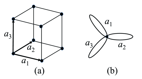
Figure 1. Simple cubic (SC) lattice

Remark 3.1.

We have the natural action of the discrete subgroup of ${\mathrm{SO}}(3)$ on the SC lattice [CS, I, Koh, S], which is isomorphic to the symmetric group $S_{4}$ on a set of four elements [I], although it does not play an important role in this article.

In this article, we often use the multiplicative abelian group

$${\mathbb{A}}_{3}:=\{\alpha_{1}^{n_{1}}\alpha_{2}^{n_{2}}\alpha_{3}^{n_{3}}\,|\,\mbox{abelian},n_{1},n_{2},n_{3}\in{\mathbb{Z}}\}$$

rather than the additive group ${\mathbb{A}}_{3}^{a}$ for convenience. Here, $\alpha_{b}$ corresponds to $a_{b}$, $b=1,2,3$. Through the natural identification of ${\mathbb{A}}_{3}$ with ${\mathbb{A}}_{3}^{a}$, we continue to use the symbols $\iota_{{\mathbb{A}}_{3}}$ and $\iota_{{\mathbb{A}}_{3},\delta}$ also for ${\mathbb{A}}_{3}$ by abuse of notation.

Remark 3.2.

The SC lattice is regarded as the universal abelian covering of a certain geometric object. In fact, the SC lattice is expressed by the graph as depicted in Figure 1 (b) [S]. More precisely, the universal abelian covering of the graph given by Figure 1 (b) coincides with the Cayley graph of the group ${\mathbb{A}}_{3}$ with respect to the generating set $\{\alpha_{1},\alpha_{2},\alpha_{3}\}$.

3.2. Fibering Structure of SC Lattice: ${(0,0,1)}$-direction

Let us introduce the group ring

$${\mathbb{C}}[{\mathbb{A}}_{3}]={\mathbb{C}}[\alpha_{1},\alpha_{2},\alpha_{3},\alpha_{1}^{-1},\alpha_{2}^{-1},\alpha_{3}^{-1}]$$

in order to consider the fibering structure of ${\mathbb{A}}_{3}$ (and that of ${\mathbb{A}}_{3}^{a}$). Its projection to the $2$-dimensional space corresponds to taking the quotient as

$${\mathbb{C}}[{\mathbb{A}}_{3}]/(\alpha_{3}-1)={\mathbb{C}}[\alpha_{1},\alpha_{2},\alpha_{1}^{-1},\alpha_{2}^{-1}]=:{\mathbb{C}}[{\mathbb{A}}_{2}],$$

where

$${\mathbb{A}}_{2}:=\{\alpha_{1}^{n_{1}}\alpha_{2}^{n_{2}}\,|\,\mbox{abelian},n_{1},n_{2}\in{\mathbb{Z}}\},$$

which is group-isomorphic to ${\mathbb{A}}_{2}^{a}:={\mathbb{Z}}a_{1}+{\mathbb{Z}}a_{2}$, and $(\alpha_{3}-1)$ is the ideal generated by $\alpha_{3}-1$. As in the case of ${\mathbb{A}}_{3}$, by assuming that $\alpha_{1}$ and $\alpha_{2}$ correspond to $(a,0)$ and $(0,a)$ in ${\mathbb{R}}^{2}$, respectively, we may regard ${\mathbb{A}}_{2}^{a}\cong{\mathbb{A}}_{2}$ as being also naturally embedded in ${\mathbb{R}}^{2}$. Thus, we have natural embeddings $\iota_{{\mathbb{A}}_{2}}:{\mathbb{A}}_{2}\hookrightarrow{\mathbb{R}}^{2}$ and $\iota_{{\mathbb{A}}_{2},\bar{\delta}}:{\mathbb{A}}_{2}\hookrightarrow{\mathbb{E}}^{2}$ defined by $\iota_{{\mathbb{A}}_{2},\bar{\delta}}(x)=\iota_{{\mathbb{A}}_{2}}(x)+\bar{\delta}$ for $\bar{\delta}=(\delta_{1},\delta_{2})\in{\mathbb{E}}^{2}$.

The projection above “induces” the fibering structure

where $\varpi$ is the projection defined by $\varpi(\alpha_{1}^{n_{1}}\alpha_{2}^{n_{2}}\alpha_{3}^{n_{3}})=\alpha_{1}^{n_{1}}\alpha_{2}^{n_{2}}$, $n_{1},n_{2},n_{3}\in{\mathbb{Z}}$. Its graph expression is given by Figure 2: more precisely, the Cayley graph of ${\mathbb{A}}_{2}$ with respect to the generating set $\{\alpha_{1},\alpha_{2},\alpha_{3}\}$ coincides with the graph depicted in Figure 2. We will see that the above fibering structure is essential in our description of screw dislocations.

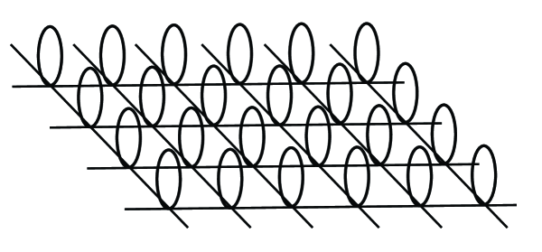
Figure 2. Fibering structure of simple cubic lattice

Note that we may regard the group ring ${\mathbb{C}}[{\mathbb{A}}_{2}]$ as a set of certain complex valued functions on ${\mathbb{A}}_{2}$: for an element of $f\in{\mathbb{C}}[{\mathbb{A}}_{2}]$, we have the complex number $f(n_{1},n_{2})\in{\mathbb{C}}$ for every element $\alpha_{1}^{n_{1}}\alpha_{2}^{n_{2}}\in{\mathbb{A}}_{2}$ in such a way that we have

$$f=\sum_{(n_{1},n_{2})\in{\mathbb{Z}}^{2}}f(n_{1},n_{2})\alpha_{1}^{n_{1}}\alpha_{2}^{n_{2}}.$$

In this case, $f$ can take non-zero complex values only on a finite number of elements of ${\mathbb{A}}_{2}$. We extend this space to the whole function space ${\mathcal{F}}({\mathcal{A}}_{p},{\mathbb{C}})$, where we use the symbol ${\mathcal{A}}_{p}$ for ${\mathbb{A}}_{2}$ viewed as a set or as a discrete topological space, i.e.,

$${\mathcal{A}}_{p}:=\{(n_{1}a,n_{2}a)\,|\,n_{1},n_{2}\in{\mathbb{Z}}\}.$$

We denote by $S^{1}_{{\mathcal{A}}_{p}}$ the trivial $S^{1}$-bundle over ${\mathcal{A}}_{p}$. For every fiber bundle $F_{{\mathbb{E}}^{2}}$ over ${\mathbb{E}}^{2}$ and for $\bar{\delta}=(\delta_{1},\delta_{2})\in{\mathbb{E}}^{2}$, by the natural embedding $\iota^{{\mathrm{SC}}}_{\bar{\delta}}:{\mathcal{A}}_{p}\hookrightarrow{\mathbb{E}}^{2}$ defined by $(n_{1}a,n_{2}a)\mapsto(n_{1}a+\delta_{1},n_{2}a+\delta_{2})$, we have the pullback bundle $F_{{\mathcal{A}}_{p}}$ over ${\mathcal{A}}_{p}$.

Let ${\mathcal{S}}={\mathcal{S}}_{+}\coprod{\mathcal{S}}_{-}$ be a finite subset in ${\mathbb{E}}^{2}$ as in Subsection 2.3. In the following, we assume that $\bar{\delta}\in{\mathbb{E}}^{2}$ satisfies $\iota^{{\mathrm{SC}}}_{\bar{\delta}}({\mathcal{A}}_{p})\cap{\mathcal{S}}=\emptyset$. Then, the map $\iota^{{\mathrm{SC}}}_{\bar{\delta}}$ is regarded as the embedding $\iota^{\mathrm{SC}}_{\bar{\delta}}:{\mathcal{A}}_{p}\hookrightarrow{\mathbb{E}}^{2}\setminus{\mathcal{S}}$. Thus, we have the following.

Lemma 3.3.

For every fiber bundle $F_{{\mathbb{E}}^{2}\setminus{\mathcal{S}}}$ over ${\mathbb{E}}^{2}\setminus{\mathcal{S}}$, by the embedding $\iota^{\mathrm{SC}}_{\bar{\delta}}:{\mathcal{A}}_{p}\hookrightarrow{\mathbb{E}}^{2}\setminus{\mathcal{S}}$, we have the pullback bundle $F_{{\mathcal{A}}_{p}}$ that satisfies the commutative diagram

where the vertical maps are the projections of the fiber bundles and $\hat{\iota}^{\mathrm{SC}}_{\bar{\delta}}$ is the bundle map induced by $\iota^{\mathrm{SC}}_{\bar{\delta}}$.

Recall that in Section 2, we have fixed $d>0$. In the following, we set $d=a$. Using the above pullback diagram (Cartesian square), we have the following.

Lemma 3.4.

We have the following commutative diagram:

where the straight vertical arrows are projections of the fiber bundles and $\widehat{\psi}$ are the bundle maps induced by $\psi$ defined in Section 2.

The above lemma is easy to prove, and hence we omit the proof.

The following proposition corresponds to the case where ${\mathcal{S}}=\emptyset$ and the proof is left to the reader.

Proposition 3.5.

Set $\gamma=\exp(2\pi{\sqrt{-1}}\delta_{3}/a)\in S^{1}$ for a $\delta_{3}\in{\mathbb{R}}$ and consider the global section $\check{\sigma}_{\gamma}\in\Gamma({\mathcal{A}}_{p},S^{1}_{{\mathcal{A}}_{p}})$ that constantly takes the value $\gamma$. Then, we have that

$$\hat{\iota}^{\mathrm{SC}}_{\bar{\delta}}\left(\widehat{\psi}^{-1}\left(\check{\sigma}_{\gamma}({\mathcal{A}}_{p})\right)\right)=\hat{\iota}^{\mathrm{SC}}_{\bar{\delta}}\left(\frac{a}{2\pi{\sqrt{-1}}}\exp^{-1}\left(\check{\sigma}_{\gamma}({\mathcal{A}}_{p})\right)\right)\subset{\mathbb{E}}_{{\mathbb{E}}^{2}\setminus{\mathcal{S}}}\subset{\mathbb{E}}^{3}$$

coincides with $\iota_{{\mathbb{A}}_{3},\delta}({\mathbb{A}}^{a}_{3})$ as a subset in ${\mathbb{E}}^{3}$ for $\delta=(\bar{\delta},\delta_{3})=(\delta_{1},\delta_{2},\delta_{3})$, i.e.,

$$\iota_{{\mathbb{A}}_{3},\delta}({\mathbb{A}}^{a}_{3})=\hat{\iota}^{\mathrm{SC}}_{\bar{\delta}}\left(\widehat{\psi}^{-1}\left(\check{\sigma}_{\gamma}({\mathcal{A}}_{p})\right)\right).$$

In other words, the SC lattice without dislocation can be interpreted as the inverse image by $\widehat{\psi}$ of a constant section $\check{\sigma}_{\gamma}$ of the trivial $S^{1}$-bundle.

3.3. Screw Dislocation in Simple Cubic Lattice

A screw dislocation in the simple cubic lattice appears along the ${(0,0,1)}$-direction [N] up to automorphisms of the SC lattice. In other words, we may assume that the Burgers vector is parallel to the $(0,0,1)$-direction.

Using the fibering structure of Lemma 3.4, for the case where ${\mathcal{S}}=\{z_{0}\}$, $z_{0}\in{\mathbb{C}}$, we can describe a single screw dislocation in the SC lattice as follows, whose proof is straightforward. Our principal idea is to use a section in $\Gamma({\mathcal{A}}_{p},S^{1}_{{\mathcal{A}}_{p}})$ in order to describe a screw dislocation. In the following, we set $z_{0}^{\prime}=z_{0}-(\delta_{1}+\delta_{2}{\sqrt{-1}})$, where $\bar{\delta}=(\delta_{1},\delta_{2})$.

Proposition 3.6.

Let us define the section $\check{\sigma}_{z_{0}^{\prime},\gamma}\in\Gamma({\mathcal{A}}_{p},S^{1}_{{\mathcal{A}}_{p}})$ by

$$\check{\sigma}_{z_{0}^{\prime},\gamma}(n_{1}a,n_{2}a)=\left(\gamma\frac{(n_{1}a+n_{2}a{\sqrt{-1}})-z_{0}^{\prime}}{|(n_{1}a+n_{2}a{\sqrt{-1}})-z_{0}^{\prime}|},(n_{1}a,n_{2}a)\right),\quad(n_{1}a,n_{2}a)\in{\mathcal{A}}_{p},$$

where $\gamma=\exp(2\pi{\sqrt{-1}}\delta_{3}/a)\in S^{1}$. Then, the screw dislocation around $z_{0}$ given by

$${\mathcal{D}}_{z_{0}}^{\mathrm{SC}}:=\hat{\iota}^{\mathrm{SC}}_{\bar{\delta}}\left(\widehat{\psi}^{-1}(\check{\sigma}_{z_{0}^{\prime},\gamma}({\mathcal{A}}_{p}))\right)=\hat{\iota}^{\mathrm{SC}}_{\bar{\delta}}\left(\frac{a}{2\pi{\sqrt{-1}}}\exp^{-1}\left(\check{\sigma}_{z_{0}^{\prime},\gamma}({\mathcal{A}}_{p})\right)\right)$$

is realized in ${\mathbb{E}}^{3}$.

We note that ${\mathcal{D}}_{z_{0}}^{\mathrm{SC}}$ can be regarded as a kind of a “covering space of the lattice ${\mathcal{A}}_{p}$”.

Remark 3.7.

(1) Let ${\mathbb{Z}}_{{\mathcal{A}}_{p},\gamma}$ be the pullback of ${\mathbb{Z}}_{{\mathbb{E}}^{2}\setminus\{z_{0}\},\gamma}$ by $\iota^{\mathrm{SC}}_{\bar{\delta}}:{\mathcal{A}}_{p}\to{\mathbb{E}}^{2}\setminus\{z_{0}\}$, and $\hat{\iota}^{\mathrm{SC}}_{\bar{\delta}}:{\mathbb{Z}}_{{\mathcal{A}}_{p},\gamma}\to{\mathbb{Z}}_{{\mathbb{E}}^{2}\setminus\{z_{0}\},\gamma}$ the induced bundle map. Then, we have the equality

$${\mathcal{D}}_{z_{0}}^{\mathrm{SC}}=\hat{\iota}^{\mathrm{SC}}_{\bar{\delta}}({\mathbb{Z}}_{{\mathcal{A}}_{p},\gamma}),$$

which follows directly from the definition of ${\mathbb{Z}}_{{\mathbb{E}}^{2}\setminus\{z_{0}\},\gamma}$ given in Subsection 2.2.

(2) Here, ${\mathcal{S}}=\{z_{0}\}$ corresponds to the position of the dislocation line (see Figure 3). As has been mentioned in the continuum model, ${\mathcal{D}}_{z_{0}}^{\mathrm{SC}}$ naturally embeds into the path space ${\mathbb{Z}}_{{\mathbb{E}}^{2}\setminus\{z_{0}\}}$ via the identification $\widehat{\varphi}_{z_{0},\delta_{3}}:{\mathbb{Z}}_{{\mathbb{E}}^{2}\setminus\{z_{0}\}}\to{\mathbb{Z}}_{{\mathbb{E}}^{2}\setminus\{z_{0}\},\gamma}$.

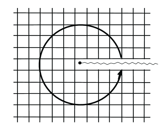
Figure 3. Screw dislocation in the SC lattice: the lattice points correspond to ${\mathcal{A}}_{p}\subset{\mathbb{E}}^{2}$ and the center point is $z_{0}$.

A parallel multi-screw dislocation is described as follows. Let us define the section $\check{\sigma}_{{\mathcal{S}}^{\prime},\gamma}\in\Gamma({\mathcal{A}}_{p},S^{1}_{{\mathcal{A}}_{p}})$ by

$$\begin{array}[]{l}\check{\sigma}_{{\mathcal{S}}^{\prime},\gamma}(n_{1}a,n_{2}a)=\\ \displaystyle{\left(\gamma\prod_{z_{i}^{\prime}\in{\mathcal{S}}_{+}^{\prime}}\frac{(n_{1}a+n_{2}a{\sqrt{-1}})-z_{i}^{\prime}}{|(n_{1}a+n_{2}a{\sqrt{-1}})-z_{i}^{\prime}|}\prod_{z_{j}^{\prime}\in{\mathcal{S}}_{-}^{\prime}}\frac{\overline{(n_{1}a+n_{2}a{\sqrt{-1}})-z_{j}^{\prime}}}{|(n_{1}a+n_{2}a{\sqrt{-1}})-z_{j}^{\prime}|},(n_{1}a,n_{2}a)\right),}\\ \hskip 256.0748pt(n_{1}a,n_{2}a)\in{\mathcal{A}}_{p},\end{array}$$

where

$$z_{i}^{\prime}=z_{i}-(\delta_{1}+\delta_{2}{\sqrt{-1}}),\,z_{j}^{\prime}=z_{j}-(\delta_{1}+\delta_{2}{\sqrt{-1}}),$$

$${\mathcal{S}}_{+}^{\prime}=\{z_{i}^{\prime}\,|\,z_{i}\in{\mathcal{S}}_{+}\},\,{\mathcal{S}}_{-}^{\prime}=\{z_{j}^{\prime}\,|\,z_{j}\in{\mathcal{S}}_{-}\}$$

and ${\mathcal{S}}^{\prime}={\mathcal{S}}_{+}^{\prime}\coprod{\mathcal{S}}_{-}^{\prime}$. Then, we have the following, whose proof is straightforward.

Proposition 3.8.

The parallel multi-screw dislocation ${\mathcal{D}}_{{\mathcal{S}}}^{\mathrm{SC}}$ given by

$${\mathcal{D}}_{{\mathcal{S}}}^{\mathrm{SC}}=\hat{\iota}^{\mathrm{SC}}_{\bar{\delta}}\left(\widehat{\psi}^{-1}(\check{\sigma}_{{\mathcal{S}}^{\prime},\gamma}({\mathcal{A}}_{p}))\right)=\hat{\iota}^{\mathrm{SC}}_{\bar{\delta}}\left(\frac{a}{2\pi{\sqrt{-1}}}\exp^{-1}(\check{\sigma}_{{\mathcal{S}}^{\prime},\gamma}({\mathcal{A}}_{p}))\right)$$

is realized in ${\mathbb{E}}^{3}$ as a subset of ${\mathbb{Z}}_{{\mathbb{E}}^{2}\setminus{\mathcal{S}},\gamma}$, where ${\mathcal{S}}$ corresponds to the position of the dislocation lines.

4. Fibering Structure of BCC Lattice: ${(1,1,1)}$-direction and its Screw Dislocation

4.1. Fibering Structure of SC Lattice: ${(1,1,1)}$-direction

In this subsection, let us first consider the fibering structure along the ${(1,1,1)}$-direction of the simple cubic lattice. Although a screw dislocation does not occur along this direction physically, this construction is useful for analyzing the case of the BCC lattice.

This structure is a little bit complicated; however, our algebraic approach makes the computation easy and enables us to have its discrete geometric interpretation. Let us consider the projection which corresponds to the quotient ring

$${\mathcal{R}_{d}}={\mathbb{C}}[{\mathbb{A}}_{3}]/(\alpha_{1}\alpha_{2}\alpha_{3}-1),$$

where ${\mathbb{A}}_{3}$ is the multiplicative free abelian group of rank $3$ generated by $\alpha_{1}$, $\alpha_{2}$ and $\alpha_{3}$.

For the vector $a_{1}+a_{2}+a_{3}\in{\mathbb{A}}_{3}^{a}\subset{\mathbb{R}}^{3}$, we have the vanishing euclidean inner products

$$(a_{1}-a_{3},a_{1}+a_{2}+a_{3})=0,\quad(a_{2}-a_{3},a_{1}+a_{2}+a_{3})=0.$$

Therefore, $a_{1}-a_{3}$ and $a_{2}-a_{3}$ constitute a basis for the orthogonal complement of the vector $a_{1}+a_{2}+a_{3}$ in ${\mathbb{R}}^{3}$. This space corresponds to the group ring generated by $\alpha_{1}\alpha_{3}^{-1}$ and $\alpha_{2}\alpha_{3}^{-1}$. In other words, we consider

$${\mathbb{A}_{d}}:=\{(\alpha_{1}\alpha_{3}^{-1})^{\ell_{1}}(\alpha_{2}\alpha_{3}^{-1})^{\ell_{2}}\,|\,\ell_{1},\ell_{2}\in{\mathbb{Z}}\},$$

which is a subgroup of ${\mathbb{A}}_{3}$. We also consider the group ring

$${\mathbb{C}}[{\mathbb{A}_{d}}]={\mathbb{C}}[\alpha_{1}\alpha_{3}^{-1},\alpha_{2}\alpha_{3}^{-1},\alpha_{1}^{-1}\alpha_{3},\alpha_{2}^{-1}\alpha_{3}],$$

which is identified, under the relation $\alpha_{1}\alpha_{2}\alpha_{3}=1$, with

$${\mathbb{C}}[\alpha_{1}\alpha_{2}^{2},\alpha_{1}^{2}\alpha_{2},\alpha_{1}^{-1}\alpha_{2}^{-2},\alpha_{1}^{-2}\alpha_{2}^{-1}].$$

Note that, as ${\mathbb{C}}[{\mathbb{A}_{d}}]$ is a sub-ring of ${\mathbb{C}}[{\mathbb{A}}_{3}]$, ${\mathcal{R}_{d}}$ is also considered to be a ${\mathbb{C}}[{\mathbb{A}_{d}}]$-module.

Lemma 4.1.

We have a natural isomorphism as ${\mathbb{C}}[{\mathbb{A}_{d}}]$-modules:

$${\mathcal{R}_{d}}\cong{\mathbb{C}}[{\mathbb{A}_{d}}]\oplus{\mathbb{C}}[{\mathbb{A}_{d}}]\alpha_{1}\oplus{\mathbb{C}}[{\mathbb{A}_{d}}]\alpha_{1}\alpha_{2}.$$

Proof.

First, note that every monomial of ${\mathbb{C}}[{\mathbb{A}}_{3}]$ has its own degree with respect to $\alpha_{1},\alpha_{2}$ and $\alpha_{3}$, each of which has degree $1$. Furthermore, it is easy to verify that a monomial has degree zero if and only if it belongs to ${\mathbb{C}}[{\mathbb{A}_{d}}]$. As a result, a monomial has degree $r$ if and only if it belongs to ${\mathbb{C}}[{\mathbb{A}_{d}}]\alpha_{1}^{r}$, where we can replace $\alpha_{1}^{r}$ by any other monomial of degree $r$. Note that each ${\mathbb{C}}[{\mathbb{A}_{d}}]\alpha_{1}^{r}$ is a ${\mathbb{C}}[{\mathbb{A}_{d}}]$-submodule of ${\mathbb{C}}[{\mathbb{A}}_{3}]$. Thus, we have the isomorphism

$${\mathbb{C}}[{\mathbb{A}}_{3}]\cong\bigoplus_{r}{\mathbb{C}}[{\mathbb{A}_{d}}]\alpha_{1}^{r}$$

as ${\mathbb{C}}[{\mathbb{A}_{d}}]$-modules.

Now, let us consider the ${\mathbb{C}}[{\mathbb{A}_{d}}]$-module homomorphism induced by the inclusion

$$q:\bigoplus_{r=0}^{2}{\mathbb{C}}[{\mathbb{A}_{d}}]\alpha_{1}^{r}\to\left.\left(\bigoplus_{r}{\mathbb{C}}[{\mathbb{A}_{d}}]\alpha_{1}^{r}\right)\right/(1-\alpha_{1}\alpha_{2}\alpha_{3})\cong{\mathbb{C}}[{\mathbb{A}}_{3}]/(1-\alpha_{1}\alpha_{2}\alpha_{3}),$$

where the ideal $(1-\alpha_{1}\alpha_{2}\alpha_{3})$ in the ring ${\mathbb{C}}[{\mathbb{A}}_{3}]$ is now considered as a ${\mathbb{C}}[{\mathbb{A}_{d}}]$-submodule. We can easily show that this homomorphism $q$ is injective, since every non-zero element of the submodule $(1-\alpha_{1}\alpha_{2}\alpha_{3})$ contains two non-zero monomials whose degrees are different by a non-zero multiple of $3$. Furthermore, $q$ is surjective, since we have ${\mathbb{C}}[{\mathbb{A}_{d}}]\alpha_{1}^{r}={\mathbb{C}}[{\mathbb{A}_{d}}]\alpha_{1}^{r^{\prime}}$ as long as $r\equiv r^{\prime}\pmod{3}$, under the relation $\alpha_{1}\alpha_{2}\alpha_{3}=1$. Furthermore, we have ${\mathbb{C}}[{\mathbb{A}_{d}}]\alpha_{1}^{2}={\mathbb{C}}[{\mathbb{A}_{d}}]\alpha_{1}\alpha_{2}$. Thus, we have the desired isomorphism of ${\mathbb{C}}[{\mathbb{A}_{d}}]$-modules. This completes the proof. ∎

Remark 4.2.

Lemma 4.1 can be geometrically interpreted by using a cube as follows. Let us consider the cube whose vertices consist of $0$, $a_{1}$, $a_{2}$, $a_{3}$, $a_{1}+a_{2}$, $a_{2}+a_{3}$, $a_{3}+a_{1}$ and $a_{1}+a_{2}+a_{3}$, which are identified with their corresponding elements $1$, $\alpha_{1}$, $\alpha_{2}$, $\alpha_{3}$, $\alpha_{1}\alpha_{2}$, $\alpha_{2}\alpha_{3}$, $\alpha_{3}\alpha_{1}$ and $\alpha_{1}\alpha_{2}\alpha_{3}$, respectively. We have the natural action of the symmetric group on the three elements $\alpha_{1}$, $\alpha_{2}$ and $\alpha_{3}$ over the cube, which can be regarded as a subgroup of the octahedral group. The orbits of this action are given by $\{1\}$, $\{\alpha_{1},\alpha_{2},\alpha_{3}\}$, $\{\alpha_{1}\alpha_{2},\alpha_{2}\alpha_{3},\alpha_{3}\alpha_{1}\}$ and $\{\alpha_{1}\alpha_{2}\alpha_{3}\}$, which coincide with the classification by their degrees. By identifying $1$ and $\alpha_{1}\alpha_{2}\alpha_{3}$, we get the three classes as described in Lemma 4.1.

Remark 4.3.

We have another algebraic proof for Lemma 4.1 as follows. Let us consider the diagonal monomorphism $\iota_{3}^{\mathrm{diag}}:{\mathbb{Z}}\hookrightarrow{\mathbb{A}}_{3}^{a}$ defined by $\iota_{3}^{\mathrm{diag}}(n)=n(a_{1}+a_{2}+a_{3})\in{\mathbb{A}}_{3}^{a}$ for $n\in{\mathbb{Z}}$, and denote its image by ${\mathbb{A}}_{3}^{\mathrm{diag}}$. Then we naturally have ${\mathcal{R}_{d}}\cong{\mathbb{C}}[{\mathbb{A}}_{3}^{a}/{\mathbb{A}}_{3}^{\mathrm{diag}}]$. Furthermore, we also have the epimorphism $p_{3}:{\mathbb{A}}_{3}^{a}\to{\mathbb{Z}}$ defined by $p_{3}(n_{1}a_{1}+n_{2}a_{2}+n_{3}a_{3})=n_{1}+n_{2}+n_{3}$ for $n_{1},n_{2},n_{3}\in{\mathbb{Z}}$. Setting ${\mathbb{A}}_{d}^{a}={\mathbb{Z}}(a_{1}-a_{3})+{\mathbb{Z}}(a_{2}-a_{3})=\mathrm{Ker}\ p_{3}$, we have the commutative diagram of exact rows

where the rightmost vertical map is the natural inclusion. By applying the snake lemma [L] to this diagram, we obtain the short exact sequence

where $\overline{p_{3}}$ is the epimorphism induced by $p_{3}$. The inverse images of the three elements of ${\mathbb{Z}}/3{\mathbb{Z}}$ by $\overline{p_{3}}$ give the decomposition of ${\mathbb{A}}_{3}^{a}/{\mathbb{A}}_{3}^{\mathrm{diag}}$ into three disjoint subsets, ${\mathbb{A}}_{d}^{a}$, $a_{1}+{\mathbb{A}}_{d}^{a}$ and $a_{1}+a_{2}+{\mathbb{A}}_{d}^{a}$. This implies Lemma 4.1.

Remark 4.4.

Lemma 4.1 means geometrically that the projection generates three sheets if we consider them embedded in ${\mathbb{E}}^{3}$ as shown in Figure 4. Each sheet can be regarded as a set given by the abelian group $\langle\alpha_{1}\alpha_{3}^{-1},\alpha_{2}\alpha_{3}^{-1}\rangle$. More precisely, let us denote ${\mathbb{A}}_{3}^{a}/{\mathbb{A}}_{3}^{\mathrm{diag}}$ by ${\mathcal{A}}_{d}$ when considered as a set. Then, we have the decomposition

$${\mathcal{A}}_{d}:={\mathcal{A}}_{d}^{(0)}\coprod{\mathcal{A}}_{d}^{(1)}\coprod{\mathcal{A}}_{d}^{(2)},$$

where

$${\mathcal{A}}_{d}^{(0)} := \{\ell_{1}(a_{1}-a_{3})+\ell_{2}(a_{2}-a_{3})\,|\,\ell_{1},\ell_{2}\in{\mathbb{Z}}\},$$

$${\mathcal{A}}_{d}^{(1)} := \{\ell_{1}(a_{1}-a_{3})+\ell_{2}(a_{2}-a_{3})+a_{1}\,|\,\ell_{1},\ell_{2}\in{\mathbb{Z}}\},$$

$${\mathcal{A}}_{d}^{(2)} := \{\ell_{1}(a_{1}-a_{3})+\ell_{2}(a_{2}-a_{3})+a_{1}+a_{2}\,|\,\ell_{1},\ell_{2}\in{\mathbb{Z}}\}.$$

Note that this corresponds exactly to the decomposition mentioned in Remark 4.3. This picture comes from the discrete nature of the lattice. The interval between the sheets is given by $\sqrt{3}a/3$.

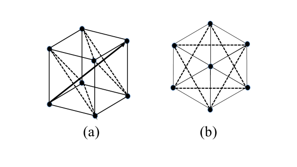
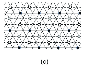
Figure 4. The cube in (a) shows the triangles whose normal direction is ${(1,1,1)}$ in simple cubic lattice. If one looks at the cube from the ${(1,1,1)}$-direction, then the image is as in (b). Furthermore, if one projects the whole SC lattice to the plane perpendicular to the ${(1,1,1)}$-direction, then one gets the image as in (c), where the black, gray and white dots correspond to the three sheets ${\mathcal{A}}_{d}^{(0)}$, ${\mathcal{A}}_{d}^{(1)}$ and ${\mathcal{A}}_{d}^{(2)}$, respectively.

4.2. Algebraic Structure of BCC Lattice

The BCC (body centered cubic) lattice is the lattice in ${\mathbb{R}}^{3}$ generated by $a_{1}$, $a_{2}$, $a_{3}$ and $(a_{1}+a_{2}+a_{3})/2$. Algebraically, it is described as additive group (or ${\mathbb{Z}}$-module) by

$${\mathbb{B}}^{a}:=\langle a_{1},a_{2},a_{3},b\rangle_{\mathbb{Z}}/\langle 2b-a_{1}-a_{2}-a_{3}\rangle_{\mathbb{Z}},$$

where $\langle 2b-a_{1}-a_{2}-a_{3}\rangle_{\mathbb{Z}}$ is the subgroup generated by $2b-a_{1}-a_{2}-a_{3}$ (see [CS, p. 116], for example). As in the case of the SC lattice, we assume that $a_{1}=(a,0,0)$, $a_{2}=(0,a,0)$, $a_{3}=(0,0,a)$ in the euclidean $3$-space ${\mathbb{E}}^{3}$ for a positive real number $a$ as shown in Figure 5 (a). The generator $b$ corresponds to the center point of the cube generated by $a_{1}$, $a_{2}$ and $a_{3}$.

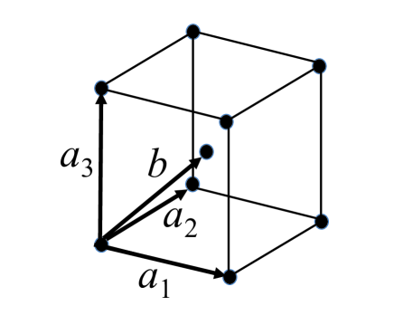
Figure 5. Body centered cubic (BCC) lattice

The lattice ${\mathbb{B}}^{a}$ is group-isomorphic to the multiplicative group

$${\mathbb{B}}:=\{\alpha_{1}^{n_{1}}\alpha_{2}^{n_{2}}\alpha_{3}^{n_{3}}\beta^{n_{4}}\,|\,\mbox{abelian},n_{1},n_{2},n_{3},n_{4}\in{\mathbb{Z}},\,\beta^{2}\alpha_{1}^{-1}\alpha_{2}^{-1}\alpha_{3}^{-1}=1\}.$$

Let us denote by ${\mathbb{A}}_{4}$ the multiplicative free abelian group of rank $4$ generated by $\alpha_{1}$, $\alpha_{2}$, $\alpha_{3}$ and $\beta$, i.e.,

$${\mathbb{A}}_{4}:=\{\alpha_{1}^{n_{1}}\alpha_{2}^{n_{2}}\alpha_{3}^{n_{3}}\beta^{n_{4}}\,|\,\mbox{abelian},\,n_{1},n_{2},n_{3},n_{4}\in{\mathbb{Z}}\}.$$

Then, ${\mathbb{B}}$ is also described as the quotient group

$${\mathbb{B}}={\mathbb{A}}_{4}/\langle\beta^{2}\alpha_{1}^{-1}\alpha_{2}^{-1}\alpha_{3}^{-1}\rangle,$$

where $\langle\beta^{2}\alpha_{1}^{-1}\alpha_{2}^{-1}\alpha_{3}^{-1}\rangle$ is the (normal) subgroup generated by $\beta^{2}\alpha_{1}^{-1}\alpha_{2}^{-1}\alpha_{3}^{-1}$. We shall consider the group ring ${\mathbb{C}}[{\mathbb{B}}]$ of ${\mathbb{B}}$,

$${\mathcal{R}_{3}}:={\mathbb{C}}[{\mathbb{B}}]={\mathbb{C}}[\alpha_{1},\alpha_{2},\alpha_{3},\alpha_{1}^{-1},\alpha_{2}^{-1},\alpha_{3}^{-1},\beta,\beta^{-1}]/(\beta^{2}-\alpha_{1}\alpha_{2}\alpha_{3}).$$

4.3. Fibering Structure of BCC Lattice

In this subsection, we consider a projection of the BCC lattice and its associated fibering structure.

As in the case of ${\mathcal{R}_{d}}$ discussed in Subsection 4.1, let us consider

$${\mathbb{B}}_{d}:=\{(\alpha_{1}\alpha_{3}^{-1})^{\ell_{1}}(\alpha_{2}\alpha_{3}^{-1})^{\ell_{2}}\,|\,\ell_{1},\ell_{2}\in{\mathbb{Z}}\},$$

which is a subgroup of ${\mathbb{B}}$. Then, we have the following decomposition as a ${\mathbb{C}}[{\mathbb{B}}_{d}]$-module.

Lemma 4.5.

We have a natural isomorphism as ${\mathbb{C}}[{\mathbb{B}}_{d}]$-modules:

$${\mathcal{R}_{3}}/(\alpha_{1}\alpha_{2}\alpha_{3}-1) \cong {\mathbb{C}}[{\mathbb{B}}_{d}]\oplus{\mathbb{C}}[{\mathbb{B}}_{d}]\alpha_{1}\oplus{\mathbb{C}}[{\mathbb{B}}_{d}]\alpha_{1}\alpha_{2}$$

$$\quad\oplus{\mathbb{C}}[{\mathbb{B}}_{d}]\beta\oplus{\mathbb{C}}[{\mathbb{B}}_{d}]\alpha_{1}\beta\oplus{\mathbb{C}}[{\mathbb{B}}_{d}]\alpha_{1}\alpha_{2}\beta.$$

We can prove the above lemma by using an argument similar to that in the proof of Lemma 4.1.

Remark 4.6.

As in Remark 4.3, we can also prove Lemma 4.5 using the snake lemma [L] as follows. First, note that we have

$${\mathcal{R}_{3}}/(\alpha_{1}\alpha_{2}\alpha_{3}-1)$$

$$\cong {\mathbb{C}}[\alpha_{1},\alpha_{2},\alpha_{3},\alpha_{1}^{-1},\alpha_{2}^{-1},\alpha_{3}^{-1},\beta,\beta^{-1}]/(\beta^{2}-\alpha_{1}\alpha_{2}\alpha_{3},\,\alpha_{1}\alpha_{2}\alpha_{3}-1)$$

$$\cong {\mathbb{C}}[\alpha_{1},\alpha_{2},\alpha_{3},\alpha_{1}^{-1},\alpha_{2}^{-1},\alpha_{3}^{-1},\beta,\beta^{-1}]/(\beta^{2}-1,\,\alpha_{1}\alpha_{2}\alpha_{3}-1)$$

$$\cong {\mathbb{C}}[\alpha_{1},\alpha_{2},\alpha_{3},\alpha_{1}^{-1},\alpha_{2}^{-1},\alpha_{3}^{-1}]/(\alpha_{1}\alpha_{2}\alpha_{3}-1)\oplus{\mathbb{C}}[\beta,\beta^{-1}]/(\beta^{2}-1).$$

Using the additive version ${\mathbb{B}}^{a}_{d}$ of the abelian multiplicative group ${\mathbb{B}}_{d}$, we have the commutative diagram with exact rows

where the rightmost vertical map and the second horizontal map in the lower sequence are the natural inclusions. By applying the snake lemma to this diagram, we obtain the relation in Lemma 4.5 as in Remark 4.3.

Thus, we have the following.

Proposition 4.7.

For

$${\mathcal{R}}:={\mathcal{R}_{3}}/(\beta-1),$$

we have a natural isomorphism as ${\mathbb{C}}[{\mathbb{B}}_{d}]$-modules:

$${\mathcal{R}}\cong{\mathbb{C}}[{\mathbb{B}}_{d}]\oplus{\mathbb{C}}[{\mathbb{B}}_{d}]\alpha_{1}\oplus{\mathbb{C}}[{\mathbb{B}}_{d}]\alpha_{1}\alpha_{2}.$$

Remark 4.8.

This corresponds to the triangle diagram for the projection of the BCC lattice, which is, in fact, the same as that depicted in Figure 4 (c). For the screw dislocation in the BCC lattice, $b\in{\mathbb{B}}$ coincides with the associated Burgers vector [N]. In other words, geometrically the “base space” corresponds to three sheets if we consider them as embedded in ${\mathbb{E}}^{3}$ as shown in Figure 4. This comes from the discrete nature of the lattice. However, the interval between the sheets is now given by $\sqrt{3}a/6$, which differs from that in the SC lattice case. More precisely, let us denote by ${\mathcal{B}}$ the subset of ${\mathbb{E}}^{3}$ corresponding to the three sheets. Then, we have

$${\mathcal{B}}:={\mathcal{B}}^{(0)}\coprod{\mathcal{B}}^{(1)}\coprod{\mathcal{B}}^{(2)},$$

where

$$\begin{array}[]{rl}{\mathcal{B}}^{(0)}&:=\{\ell_{1}(a_{1}-a_{3})+\ell_{2}(a_{2}-a_{3})\,|\,\ell_{1},\ell_{2}\in{\mathbb{Z}}\},\\ {\mathcal{B}}^{(1)}&:=\{\ell_{1}(a_{1}-a_{3})+\ell_{2}(a_{2}-a_{3})+a_{1}-b\,|\,\ell_{1},\ell_{2}\in{\mathbb{Z}}\},\\ {\mathcal{B}}^{(2)}&:=\{\ell_{1}(a_{1}-a_{3})+\ell_{2}(a_{2}-a_{3})+a_{1}+a_{2}-b\,|\,\ell_{1},\ell_{2}\in{\mathbb{Z}}\}.\\ \end{array}$$

By observing that the degree of $b$ is equal to $3/2$, we see that the three sheets above correspond to the classification by the degrees (modulo $3/2$).

Thus, we have the following.

Lemma 4.9.

As a set, ${\mathbb{B}}^{a}$ is also decomposed as

$${\mathbb{B}}^{a}={\mathbb{B}}^{(0)}\coprod{\mathbb{B}}^{(1)}\coprod{\mathbb{B}}^{(2)},$$

where

$$\begin{array}[]{rl}{\mathbb{B}}^{(0)}&:=\{\ell_{1}(a_{1}-a_{3})+\ell_{2}(a_{2}-a_{3})+\ell_{3}b\,|\,\ell_{1},\ell_{2},\ell_{3}\in{\mathbb{Z}}\},\\ {\mathbb{B}}^{(1)}&:=\{\ell_{1}(a_{1}-a_{3})+\ell_{2}(a_{2}-a_{3})+a_{1}+\ell_{3}b\,|\,\ell_{1},\ell_{2},\ell_{3}\in{\mathbb{Z}}\},\\ {\mathbb{B}}^{(2)}&:=\{\ell_{1}(a_{1}-a_{3})+\ell_{2}(a_{2}-a_{3})+a_{1}+a_{2}+\ell_{3}b\,|\,\ell_{1},\ell_{2},\ell_{3}\in{\mathbb{Z}}\}.\\ \end{array}$$

Let $\eta:{\mathbb{R}}^{3}\to{\mathbb{R}}^{3}$ be the orthogonal transformation that sends $a_{1}$, $a_{2}$ and $a_{3}$ to the vectors

$$a\!\left(\begin{array}[]{c}\sqrt{2}/2\\ -\sqrt{6}/6\\ \sqrt{3}/3\end{array}\right),\,a\!\left(\begin{array}[]{c}0\\ \sqrt{6}/3\\ \sqrt{3}/3\end{array}\right)\,\mbox{\rm and }\,a\!\left(\begin{array}[]{c}-\sqrt{2}/2\\ -\sqrt{6}/6\\ \sqrt{3}/3\end{array}\right),$$

respectively. For a vector $\delta=(\delta_{1},\delta_{2},\delta_{3})\in{\mathbb{E}}^{3}$, we consider the embedding

$$\iota^{\mathrm{BCC}}_{\delta}:{\mathbb{B}}^{a}\hookrightarrow{\mathbb{E}}^{3}$$

defined by $x\mapsto\eta(x)+\delta$ for $x\in{\mathbb{B}}^{a}\subset{\mathbb{R}}^{3}$. Note that $\eta$ sends the vector $2b=a(1,1,1)$ to $\sqrt{3}a(0,0,1)$, and therefore $\iota^{\mathrm{BCC}}_{\delta}$ sends each ${\mathbb{B}}^{(c)}$ into a plane parallel to the plane spanned by $(1,0,0)$ and $(0,1,0)$ for $c=0,1,2$.

Let $\pi:{\mathbb{E}}^{3}\to{\mathbb{E}}^{2}$ be the natural projection to the first and second coordinates. As in the case of ${\mathcal{A}}_{d}$, we consider the natural embedding $\iota^{{\mathrm{BCC}},c}_{\bar{\delta}}=\pi\circ\iota^{\mathrm{BCC}}_{\delta}|{\mathcal{B}}^{(c)}:{\mathcal{B}}^{(c)}={\mathbb{Z}}^{2}\hookrightarrow{\mathbb{E}}^{2}$, $c=0,1,2$, where $\bar{\delta}=(\delta_{1},\delta_{2})\in{\mathbb{E}}^{2}$.

With the help of Figure 6, we can prove the following lemma.

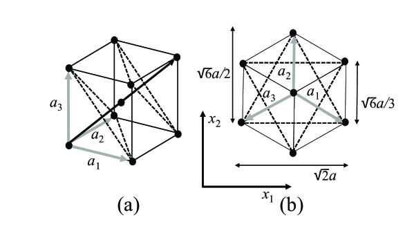
Figure 6. Body centered cubic lattice and its projection along the ${(1,1,1)}$-direction

Lemma 4.10.

For the embedding $\iota^{{\mathrm{BCC}},c}_{\bar{\delta}}:{\mathcal{B}}^{(c)}\hookrightarrow{\mathbb{E}}^{2}$, $c=0,1,2$, we have the following:

$$\iota^{{\mathrm{BCC}},0}_{\bar{\delta}}(x) = (\sqrt{2}\ell_{1}a+\sqrt{2}\ell_{2}a/2,\sqrt{6}\ell_{2}a/2)+\bar{\delta}$$

$$\qquad\mbox{\rm for }x=\ell_{1}(a_{1}-a_{3})+\ell_{2}(a_{2}-a_{3})\in{\mathcal{B}}^{(0)},$$

$$\iota^{{\mathrm{BCC}},1}_{\bar{\delta}}(x) = (\sqrt{2}\ell_{1}a+\sqrt{2}a/2+\sqrt{2}\ell_{2}a/2,(\sqrt{6}\ell_{2}a-\sqrt{6}a/3)/2)+\bar{\delta}$$

$$\qquad\mbox{\rm for }x=\ell_{1}(a_{1}-a_{3})+\ell_{2}(a_{2}-a_{3})+a_{1}-b\in{\mathcal{B}}^{(1)},$$

$$\iota^{{\mathrm{BCC}},2}_{\bar{\delta}}(x) = (\sqrt{2}\ell_{1}a+\sqrt{2}a/2+\sqrt{2}\ell_{2}a/2,(\sqrt{6}\ell_{2}a+2\sqrt{6}a/3)/2)+\bar{\delta}$$

$$\qquad\mbox{\rm for }x=\ell_{1}(a_{1}-a_{3})+\ell_{2}(a_{2}-a_{3})+a_{1}+a_{2}-b\in{\mathcal{B}}^{(2)}.$$

Let ${\mathcal{S}}={\mathcal{S}}_{+}\coprod{\mathcal{S}}_{-}$ be a finite subset in ${\mathbb{E}}^{2}$ as in Subsection 2.3. In the following, we assume that $\bar{\delta}\in{\mathbb{E}}^{2}$ satisfies $\iota^{{\mathrm{BCC}},c}_{\bar{\delta}}({\mathcal{B}}^{(c)})\cap{\mathcal{S}}=\emptyset$, $c=0,1,2$. Then, we have the following, whose proof is straightforward.

Lemma 4.11.

For every fiber bundle $F_{{\mathbb{E}}^{2}\setminus{\mathcal{S}}}$ over ${\mathbb{E}}^{2}\setminus{\mathcal{S}}$, by the embedding $\iota^{{\mathrm{BCC}},c}_{\bar{\delta}}:{\mathcal{B}}^{(c)}\hookrightarrow{\mathbb{E}}^{2}\setminus{\mathcal{S}}$, $c=0,1,2$, we have the pullback bundle $F_{{\mathcal{B}}^{(c)}}$ that satisfies the commutative diagram

where the vertical maps are the projections of the fiber bundles and $\hat{\iota}^{{\mathrm{BCC}},c}_{\bar{\delta}}$ is the bundle map induced by $\iota^{{\mathrm{BCC}},c}_{\bar{\delta}}$.

Using this pullback diagram (Cartesian square), we have the following, whose proof is straightforward.

Lemma 4.12.

We have the following commutative diagram:

for $c=0,1,2$, where ${\mathbb{E}}_{{\mathcal{B}}^{(c)}}$ and $S^{1}_{{\mathcal{B}}^{(c)}}$ are the trivial bundles, the straight vertical arrows are projections of the fiber bundles, $\widehat{\psi}$ are the bundle maps induced by $\psi$ defined in Section 2, and the positive constant $d$ in Section 2 is now set $d=\sqrt{3}a/2$, which $\widehat{\psi}$ depends on.

The following proposition corresponds to the case where ${\mathcal{S}}=\emptyset$ and the proof is left to the reader.

Proposition 4.13.

Set $\gamma=\exp(4\pi{\sqrt{-1}}\delta_{3}/(\sqrt{3}a))\in S^{1}$ and consider the global sections

$$\tilde{\sigma}_{\gamma,c}\in\Gamma({\mathcal{B}}^{(c)},S^{1}_{{\mathcal{B}}^{(c)}}),\quad c=0,1,2,$$

that constantly take the values $\gamma\zeta_{3}^{-c}$, where $\zeta_{3}=\exp(2\pi{\sqrt{-1}}/3)$. Then, we have

$$\iota^{{\mathrm{BCC}}}_{\delta}({\mathbb{B}}^{a})=\bigcup_{c=0}^{2}\hat{\iota}^{{\mathrm{BCC}},c}_{\bar{\delta}}\left(\widehat{\psi}^{-1}\left(\tilde{\sigma}_{\gamma,c}({\mathcal{B}}^{(c)})\right)\right)\subset{\mathbb{E}}^{3}.$$

4.4. Algebraic Description of Screw Dislocations in BCC Lattice

Recall that a screw dislocation in the BCC lattice is basically given by the ${(1,1,1)}$-direction. In other words, the Burgers vector is parallel to the ${(1,1,1)}$-direction, or more precisely it coincides with $b$ itself, up to automorphisms of the BCC lattice [N].

In the following, for $\gamma^{\prime}\in S^{1}$ and $\tilde{\sigma}\in\Gamma({\mathcal{B}},S^{1}_{{\mathcal{B}}})$ expressed as $\tilde{\sigma}(x)=(s(x),x)$ for $x\in{\mathcal{B}}$, we define their multiplication $\gamma^{\prime}\tilde{\sigma}\in\Gamma({\mathcal{B}},S^{1}_{{\mathcal{B}}})$ by $(\gamma^{\prime}\tilde{\sigma})(x)=(\gamma^{\prime}s(x),x)$, $x\in{\mathcal{B}}$, where $S^{1}_{{\mathcal{B}}}$ is the trivial $S^{1}$-bundle over ${\mathcal{B}}$.

Now, as in Proposition 3.6 for the SC lattice case, we have the following description of a single screw dislocation in the BCC lattice. In the following, we set $z_{0}^{\prime}=z_{0}-(\delta_{1}+\delta_{2}{\sqrt{-1}})$.

Proposition 4.14.

The single screw dislocation expressed by

$$\bigcup_{c=0}^{2}\hat{\iota}^{{\mathrm{BCC}},c}_{\bar{\delta}}\left(\widehat{\psi}^{-1}\left((\gamma\zeta_{3}^{-c}\tilde{\sigma}_{z_{0}^{\prime}})({\mathcal{B}}^{(c)})\right)\right)$$

around $z_{0}\in{\mathbb{E}}^{2}$ is a subset of ${\mathbb{E}}^{3}$, where $\tilde{\sigma}_{z_{0}^{\prime}}$ is an element of $\Gamma({\mathcal{B}},S^{1}_{{\mathcal{B}}})$ given by

$$\begin{array}[]{l}\tilde{\sigma}_{z_{0}^{\prime}}(x)=\\ \displaystyle{\left(\frac{\sqrt{2}\ell_{1}a+\sqrt{2}\ell_{2}a/2-x_{0}^{\prime}+(\sqrt{6}\ell_{2}a/2-y_{0}^{\prime}){\sqrt{-1}}}{|\sqrt{2}\ell_{1}a+\sqrt{2}\ell_{2}a/2-x_{0}^{\prime}+(\sqrt{6}\ell_{2}a/2-y_{0}^{\prime}){\sqrt{-1}}|},x\right)}\\ \qquad\mbox{\rm for }x=\ell_{1}(a_{1}-a_{3})+\ell_{2}(a_{2}-a_{3})\in{\mathcal{B}}^{(0)},\\ \\ \tilde{\sigma}_{z_{0}^{\prime}}(x)=\\ \displaystyle{\left(\frac{\sqrt{2}\ell_{1}a+\sqrt{2}a/2+\sqrt{2}\ell_{2}a/2-x_{0}^{\prime}+((\sqrt{6}\ell_{2}a-\sqrt{6}a/3)/2-y_{0}^{\prime}){\sqrt{-1}}}{|\sqrt{2}\ell_{1}a+\sqrt{2}a/2+\sqrt{2}\ell_{2}a/2-x_{0}^{\prime}+((\sqrt{6}\ell_{2}a-\sqrt{6}a/3)/2-y_{0}^{\prime}){\sqrt{-1}}|},x\right)}\\ \quad\mbox{\rm for }x=\ell_{1}(a_{1}-a_{3})+\ell_{2}(a_{2}-a_{3})+a_{1}-b\in{\mathcal{B}}^{(1)},\\ \\ \tilde{\sigma}_{z_{0}^{\prime}}(x)=\\ \displaystyle{\left(\frac{\sqrt{2}\ell_{1}a+\sqrt{2}a/2+\sqrt{2}\ell_{2}a/2-x_{0}^{\prime}(+((\sqrt{6}\ell_{2}a+2\sqrt{6}a/3)/2-y_{0}^{\prime}){\sqrt{-1}}}{|\sqrt{2}\ell_{1}a+\sqrt{2}a/2+\sqrt{2}\ell_{2}a/2-x_{0}^{\prime}+((\sqrt{6}\ell_{2}a+2\sqrt{6}a/3)/2-y_{0}^{\prime}){\sqrt{-1}}|},x\right)}\\ \quad\mbox{\rm for }x=\ell_{1}(a_{1}-a_{3})+\ell_{2}(a_{2}-a_{3})+a_{1}+a_{2}-b\in{\mathcal{B}}^{(2)},\end{array}$$

where $z_{0}^{\prime}=x_{0}^{\prime}+y_{0}^{\prime}{\sqrt{-1}}\in{\mathbb{C}}$ and $(\ell_{1},\ell_{2})\in{\mathbb{Z}}^{2}$.

Furthermore, for $\tilde{\sigma}_{1}$ and $\tilde{\sigma}_{2}\in\Gamma({\mathcal{B}},S^{1}_{{\mathcal{B}}})$ expressed as $\tilde{\sigma}_{a}(x)=(s_{a}(x),x)$ for $x\in{\mathcal{B}}$, $a=1,2$, we define their multiplication $\tilde{\sigma}_{1}\tilde{\sigma}_{2}$ by $(\tilde{\sigma}_{1}\tilde{\sigma}_{2})(x)=(s_{1}(x)s_{2}(x),x)$, $x\in{\mathcal{B}}$. Using the multiplication, we have the following description of a parallel multi-screw dislocation in the BCC lattice.

Proposition 4.15.

The parallel multi-screw dislocation in the BCC lattice given by

$$\bigcup_{c=0}^{2}\hat{\iota}^{{\mathrm{BCC}},c}_{\bar{\delta}}\left(\widehat{\psi}^{-1}\left(\left(\gamma\zeta_{3}^{-c}\prod_{z_{i}^{\prime}\in{\mathcal{S}}_{+}^{\prime}}\tilde{\sigma}_{z_{i}^{\prime}}\prod_{z_{j}^{\prime}\in{\mathcal{S}}_{-}^{\prime}}\overline{\tilde{\sigma}_{z_{j}^{\prime}}}\right)({\mathcal{B}}^{(c)})\right)\right)$$

$$= \bigcup_{c=0}^{2}\hat{\iota}^{{\mathrm{BCC}},c}_{\bar{\delta}}\left(\frac{\sqrt{3}a}{4\pi{\sqrt{-1}}}\exp^{-1}\left(\left(\gamma\zeta_{3}^{-c}\prod_{z_{i}^{\prime}\in{\mathcal{S}}_{+}^{\prime}}\tilde{\sigma}_{z_{i}^{\prime}}\prod_{z_{j}^{\prime}\in{\mathcal{S}}_{-}^{\prime}}\overline{\tilde{\sigma}_{z_{j}^{\prime}}}\right)({\mathcal{B}}^{(c)})\right)\right)$$

is a subset of ${\mathbb{E}}^{3}$, where ${\mathcal{S}}$ corresponds to the position of the dislocation lines, $z_{i}^{\prime}=z_{i}-(\delta_{1}+\delta_{2}{\sqrt{-1}})$, $z_{j}^{\prime}=z_{j}-(\delta_{1}+\delta_{2}{\sqrt{-1}})$, ${\mathcal{S}}_{+}^{\prime}=\{z_{i}^{\prime}\,|\,z_{i}\in{\mathcal{S}}_{+}\}$, ${\mathcal{S}}_{-}^{\prime}=\{z_{j}^{\prime}\,|\,z_{j}\in{\mathcal{S}}_{-}\}$ and ${\mathcal{S}}^{\prime}={\mathcal{S}}_{+}^{\prime}\coprod{\mathcal{S}}_{-}^{\prime}$.

In Subsection 7.1, we will give a more explicit formula for a single screw dislocation.

5. Energy of Screw Dislocation

5.1. Energy of Screw Dislocation in SC Lattice

In this section, we consider the strain energy of a single screw dislocation in the SC lattice along the ${(0,0,1)}$-direction as discussed in Subsection 3.3. We adopt a spring model, in which certain “edges” of the SC lattice correspond to elastic springs, whose natural lengths are equal to $a$ or $\sqrt{2}a$.

More precisely, in our model, we have the elastic springs on the edges

$$[(n_{1},n_{2},n_{3}),(n_{1}+1,n_{2},n_{3})],\quad[(n_{1},n_{2},n_{3}),(n_{1},n_{2}+1,n_{3})],$$

$$[(n_{1},n_{2},n_{3}),(n_{1},n_{2},n_{3}+1)],\quad[(n_{1},n_{2},n_{3}),(n_{1}+1,n_{2},n_{3}\pm 1)],$$

$$[(n_{1},n_{2},n_{3}),(n_{1},n_{2}+1,n_{3}\pm 1)],\quad[(n_{1},n_{2},n_{3}),(n_{1}+1,n_{2}\pm 1,n_{3})],$$

for all $(n_{1},n_{2},n_{3})\in{\mathbb{Z}}^{3}$. Note that the above parametrization refers to a local one for the SC lattice after the dislocation, in a neighborhood of each vertex sufficiently far from the dislocation line. It is clear that such a parametrization does not work globally; however, around each point, such a parametrization works as long as the point is far from the dislocation center. In this section we will use this parameterization for simplicity and compute the strain energy caused by a screw dislocation.

We note that there are several other possibilities for the choice of the edges. The choice of the model, however, does not affect the essentials of the results, as we will see later.

Now, let us consider the screw dislocation in the SC lattice along the ${(0,0,1)}$-direction around $z_{0}\in{\mathbb{C}}$, as described in Subsection 3.3. For simplicity, throughout this section, we suppose $\delta=(0,0,0)$ and $\bar{\delta}=(0,0)$ so that $z_{0}^{\prime}=z_{0}$. Furthermore, we assume that $z_{0}=x_{0}+y_{0}{\sqrt{-1}}$, $x_{0},y_{0}\in{\mathbb{R}}$, satisfies that $x_{0},y_{0}$ and $\pm x_{0}\pm y_{0}$ are not integral multiples of $a$. We regard that the original lattice is in a stable position, and we consider the elastic energy resulting from the dislocation. For this, we need to investigate the difference between the original position and the position resulting from the dislocation.

In the following, we also assume that $\gamma=1$ for simplicity. For notational convention, we will denote $\check{\sigma}_{z_{0},\gamma}$ etc. simply by $\check{\sigma}_{z_{0}}$ etc. by suppressing $\gamma$.

First, we define the relative height differences $\epsilon_{n_{1},n_{2}}^{(1)}$, $\epsilon_{n_{1},n_{2}}^{(2)}$ and $\epsilon_{n_{1},n_{2}}^{(\pm)}$ by

(5.1) $$\begin{array}[]{rl}\displaystyle{\epsilon_{n_{1},n_{2}}^{(1)}}&\displaystyle{=\frac{a}{2\pi{\sqrt{-1}}}\left(\log(\check{\sigma}_{z_{0}}((n_{1}+1)a,n_{2}a))-\log(\check{\sigma}_{z_{0}}(n_{1}a,n_{2}a))\right),}\raisebox{0.0pt}[19.91692pt][19.91692pt]{}\\ \displaystyle{\epsilon_{n_{1},n_{2}}^{(2)}}&\displaystyle{=\frac{a}{2\pi{\sqrt{-1}}}\left(\log(\check{\sigma}_{z_{0}}(n_{1}a,(n_{2}+1)a))-\log(\check{\sigma}_{z_{0}}(n_{1}a,n_{2}a))\right),}\raisebox{0.0pt}[19.91692pt][19.91692pt]{}\\ \displaystyle{\epsilon_{n_{1},n_{2}}^{(\pm)}}&\displaystyle{=\frac{a}{2\pi{\sqrt{-1}}}\left(\log(\check{\sigma}_{z_{0}}((n_{1}+1)a,(n_{2}\pm 1)a))-\log(\check{\sigma}_{z_{0}}(n_{1}a,n_{2}a))\right),}\\ \end{array}$$

respectively, where $\log x=\log_{e}x$ for $x\in S^{1}$ is considered to be ${\sqrt{-1}}$ times the argument of $x$, and we choose the values so that $-a/2<\epsilon_{n_{1},n_{2}}^{(i)}\leq a/2$ for $i=1,2$ and $\pm$. Later we will see that it never takes the value $a/2$.

In what follows, for a section $\check{\sigma}\in\Gamma({\mathcal{A}}_{p},S^{1}_{{\mathcal{A}}_{p}})$ expressed as $\check{\sigma}(x)=(s(x),x)$ for $x\in{\mathcal{A}}_{p}$, we often use the symbol $\check{\sigma}(x)$ instead of $s(x)$ by abuse of notation. We recall that

$$\check{\sigma}_{z_{0}}(n_{1}a,n_{2}a)={\check{\sigma}_{z_{0},\gamma}(n_{1}a,n_{2}a)}=\frac{n_{1}a-x_{0}+(n_{2}a-y_{0}){\sqrt{-1}}}{\left|n_{1}a-x_{0}+(n_{2}a-y_{0}){\sqrt{-1}}\right|}$$

for $z_{0}=x_{0}+y_{0}{\sqrt{-1}}$, $x_{0},y_{0}\in{\mathbb{R}}$, and $\gamma=1$ in Proposition 3.6. Set $z=n_{1}a-x_{0}+(n_{2}a-y_{0}){\sqrt{-1}}$, which is not a real multiple of $1,{\sqrt{-1}}$ or $1\pm{\sqrt{-1}}$ by our assumption on $z_{0}$. Then, we get

(5.2) $$\begin{array}[]{rl}\displaystyle{\epsilon_{n_{1},n_{2}}^{(1)}}&\displaystyle{=\frac{a}{2\pi{\sqrt{-1}}}\log\frac{1+a/z}{|1+a/z|},}\raisebox{0.0pt}[19.91692pt][19.91692pt]{}\\ \displaystyle{\epsilon_{n_{1},n_{2}}^{(2)}}&\displaystyle{=\frac{a}{2\pi{\sqrt{-1}}}\log\frac{1+a{\sqrt{-1}}/z}{|1+a{\sqrt{-1}}/z|},}\raisebox{0.0pt}[19.91692pt][19.91692pt]{}\\ \displaystyle{\epsilon_{n_{1},n_{2}}^{(\pm)}}&\displaystyle{=\frac{a}{2\pi{\sqrt{-1}}}\log\frac{1+a(1\pm{\sqrt{-1}})/z}{|1+a(1\pm{\sqrt{-1}})/z|}}.\\ \end{array}$$

Note that $1+a/z$, $1+a{\sqrt{-1}}/z$ and $1+a(1\pm{\sqrt{-1}})/z$ have non-zero imaginary parts, and therefore $\epsilon_{n_{1},n_{2}}^{(i)}$ never takes the value $a/2$ for $i=1,2$ and $\pm$.

Then, the difference of length in each segment

$$[(n_{1},n_{2},n_{3}),(n_{1}+1,n_{2},n_{3})]\quad\mbox{\rm or}\quad[(n_{1},n_{2},n_{3}),(n_{1},n_{2}+1,n_{3})]$$

is given by

$$\Delta_{n_{1},n_{2}}^{(i)}=\sqrt{a^{2}+(\epsilon_{n_{1},n_{2}}^{(i)})^{2}}-a,$$

$i=1,2$, whereas the difference of length in each diagonal segment

$$[(n_{1},n_{2},n_{3}),(n_{1}+1,n_{2},n_{3}\pm 1)]\quad\mbox{\rm or}\quad[(n_{1},n_{2},n_{3}),(n_{1},n_{2}+1,n_{3}\pm 1)]$$

is given by

(5.3) $$\Delta_{n_{1},n_{2}}^{d(i,\pm)}=\sqrt{(a\pm\epsilon_{n_{1},n_{2}}^{(i)})^{2}+a^{2}}-\sqrt{2}a,$$

$i=1,2$, and the difference of length in the diagonal segment

$$[(n_{1},n_{2},n_{3}),(n_{1}+1,n_{2}\pm 1,n_{3})]$$

is given by

(5.4) $$\Delta_{n_{1},n_{2}}^{d(\pm)}=\sqrt{2a^{2}+(\epsilon_{n_{1},n_{2}}^{(\pm)})^{2}}-\sqrt{2}a.$$

On the other hand, the length of the segment $[(n_{1},n_{2},n_{3}),(n_{1},n_{2},n_{3}+1)]$ is constantly equal to the natural length $a$ and thus we set $\Delta_{n_{1},n_{2}}^{(3)}=0$.

Then, we have the following.

Lemma 5.1.

If

$$\frac{a}{\sqrt{(n_{1}a-x_{0})^{2}+(n_{2}a-y_{0})^{2}}}$$

is sufficiently small, then $\epsilon^{(1)}_{n_{1},n_{2}}$, $\epsilon^{(2)}_{n_{1},n_{2}}$ and $\epsilon^{(\pm)}_{n_{1},n_{2}}$ are approximately given by

$$\epsilon_{n_{1},n_{2}}^{(1)} = -\frac{a}{2\pi}\frac{a(n_{2}a-y_{0})}{(n_{1}a-x_{0})^{2}+(n_{2}a-y_{0})^{2}}$$

$$\qquad\qquad\qquad+o\left(\frac{a}{\sqrt{(n_{1}a-x_{0})^{2}+(n_{2}a-y_{0})^{2}}}\right),$$

(5.5) $$\epsilon_{n_{1},n_{2}}^{(2)} = -\frac{a}{2\pi}\frac{a(n_{1}a-x_{0})}{(n_{1}a-x_{0})^{2}+(n_{2}a-y_{0})^{2}}$$

$$\qquad\qquad\qquad+o\left(\frac{a}{\sqrt{(n_{1}a-x_{0})^{2}+(n_{2}a-y_{0})^{2}}}\right),$$

$$\epsilon_{n_{1},n_{2}}^{(\pm)} = -\frac{a}{2\pi}\frac{\pm a(n_{1}a-x_{0})+a(n_{2}a-y_{0})}{(n_{1}a-x_{0})^{2}+(n_{2}a-y_{0})^{2}}$$

$$\qquad\qquad\qquad+o\left(\frac{a}{\sqrt{(n_{1}a-x_{0})^{2}+(n_{2}a-y_{0})^{2}}}\right),$$

respectively, whereas $\Delta_{n_{1},n_{2}}^{(i)}$ $\Delta_{n_{1},n_{2}}^{d(i,\pm)}$ and $\Delta_{n_{1},n_{2}}^{d(\pm)}$ are approximately given by

(5.6) $$\begin{array}[]{l}\displaystyle{\Delta_{n_{1},n_{2}}^{(i)}=\frac{1}{2a}(\epsilon_{n_{1},n_{2}}^{(i)})^{2}+o\left(\frac{a}{\sqrt{(n_{1}a-x_{0})^{2}+(n_{2}a-y_{0})^{2}}}\right),}\raisebox{0.0pt}[19.91692pt][19.91692pt]{}\\ \displaystyle{\Delta_{n_{1},n_{2}}^{d(i,\pm)}=\pm\frac{1}{\sqrt{2}}\epsilon_{n_{1},n_{2}}^{(i)}+o\left(\frac{a}{\sqrt{(n_{1}a-x_{0})^{2}+(n_{2}a-y_{0})^{2}}}\right),}\raisebox{0.0pt}[19.91692pt][19.91692pt]{}\\ \displaystyle{\Delta_{n_{1},n_{2}}^{d(\pm)}=\frac{1}{2\sqrt{2}a}(\epsilon_{n_{1},n_{2}}^{(\pm)})^{2}+o\left(\frac{a}{\sqrt{(n_{1}a-x_{0})^{2}+(n_{2}a-y_{0})^{2}}}\right),}\end{array}$$

respectively, $i=1,2$.

Proof.

Setting

$$z:=(n_{1}a-x_{0})+(n_{2}a-y_{0}){\sqrt{-1}},$$

we have

$$\check{\sigma}_{z_{0}}((n_{1}+1)a,n_{2}a) = {\displaystyle\frac{z+a}{\left|z+a\right|}}=\check{\sigma}_{z_{0}}(n_{1}a,n_{2}a){\displaystyle\frac{1+a/z}{\left|1+a/z\right|}},$$

$$\check{\sigma}_{z_{0}}(n_{1}a,(n_{2}+1)a) = {\displaystyle\frac{z+a{\sqrt{-1}}}{\left|z+a{\sqrt{-1}}\right|}}=\check{\sigma}_{z_{0}}(n_{1}a,n_{2}a){\displaystyle\frac{1+a{\sqrt{-1}}/z}{\left|1+a{\sqrt{-1}}/z\right|}},$$

$$\check{\sigma}_{z_{0}}((n_{1}+1)a,(n_{2}\pm 1)a) = {\displaystyle\frac{z+a\pm a{\sqrt{-1}}}{\left|z+a\pm a{\sqrt{-1}}\right|}}$$

$$= \check{\sigma}_{z_{0}}(n_{1}a,n_{2}a){\displaystyle\frac{1+a(1\pm{\sqrt{-1}})/z}{\left|1+a(1\pm{\sqrt{-1}})/z\right|}}.$$

By Taylor expansion, we have, for $w=\xi+\xi^{\prime}{\sqrt{-1}}$, $\xi,\xi^{\prime}\in{\mathbb{R}}$,

$$\arg(1+w)=\arctan{\displaystyle\frac{\xi^{\prime}}{1+\xi}}=\xi^{\prime}+o(\left|w\right|)$$

as $w\to 0$. Therefore, we obtain that

$$\begin{array}[]{rl}\arg\left(1+{\displaystyle\frac{a}{z}}\right)&=\mathop{\mathrm{Im}}{\displaystyle\frac{a}{z}}+o\left({\displaystyle\frac{a}{\left|z\right|}}\right)\\ &=-{\displaystyle\frac{a}{\left|z\right|^{2}}}(n_{2}a-y_{0})+o\left({\displaystyle\frac{a}{\left|z\right|}}\right),\\ \arg\left(1+{\displaystyle\frac{a{\sqrt{-1}}}{z}}\right)&=\mathop{\mathrm{Re}}{\displaystyle\frac{a}{z}}+o\left({\displaystyle\frac{a}{\left|z\right|}}\right)\\ &={\displaystyle\frac{a}{\left|z\right|^{2}}}(n_{1}a-x_{0})+o\left({\displaystyle\frac{a}{\left|z\right|}}\right),\\ \arg\left(1+{\displaystyle\frac{a(1\pm{\sqrt{-1}})}{z}}\right)&=\mathop{\mathrm{Im}}{\displaystyle\frac{a}{z}}\pm\mathop{\mathrm{Re}}{\displaystyle\frac{a}{z}}+o\left({\displaystyle\frac{a}{\left|z\right|}}\right)\\ &={\displaystyle\frac{a}{\left|z\right|^{2}}}\left(-(n_{2}a-y_{0})\pm(n_{1}a-x_{0})\right)+o\left({\displaystyle\frac{a}{\left|z\right|}}\right).\\ \end{array}$$

Then, we get the approximation formula (5.5) from definition (5.1).

Finally, we can prove the approximation formula (5.6) for $\Delta_{n_{1},n_{2}}^{(i)}$, $\Delta_{n_{1},n_{2}}^{d(i,\pm)}$, $i=1,2$, and $\Delta_{n_{1},n_{2}}^{d(\pm)}$ by simple application of the Taylor expansion. This completes the proof. ∎

Following the spirit of the theory of elasticity [LL, M], in the following, we assume that

$$\frac{a}{\sqrt{(n_{1}a-x_{0})^{2}+(n_{2}a-y_{0})^{2}}}=\frac{a}{|z|}$$

is small in Lemma 5.1 and in particular $a/|z|<1/\sqrt{2}$. This assumption means that the node $(n_{1}a,n_{2}a)$ in ${\mathbb{E}}^{2}$ is sufficiently far from the center $(x_{0},y_{0})$ of dislocation relative to the lattice length $a$. Such an approximation does not hold for the nodes near the center. More explicitly, the approximation given above is valid for the elastic energy in the far region

(5.7) $$A_{\rho}:=\left\{(n_{1},n_{2})\in{\mathbb{Z}}^{2}\,|\,\rho a<\sqrt{(n_{1}a-x_{0})^{2}+(n_{2}a-y_{0})^{2}}\right\}$$

for sufficiently large fixed $\rho\geq\sqrt{2}$. On the other hand, in the core region ${\mathbb{Z}}^{2}\setminus A_{\rho}$, the approximation fails and we need to adopt another approach.

Furthermore, for later convenience, let us introduce the notation

(5.8) $$A_{\rho,N}:=\left\{(n_{1},n_{2})\in{\mathbb{Z}}^{2}\,|\,\rho a<\sqrt{(n_{1}a-x_{0})^{2}+(n_{2}a-y_{0})^{2}}<Na\right\}$$

for $N>\rho$, which is bounded and is a finite set.

We can now compute the elastic energy caused by the screw dislocation. Since our model has the translational symmetry along the $(0,0,1)$-axis (i.e., the set of lattice points $(n_{1},n_{2},n_{3})$ together with the edges with springs in our model is invariant under the translation $n_{3}\mapsto n_{3}+1$), we will concentrate ourselves on the energy density for unit length in the $(0,0,1)$-direction, and call it simply the elastic energy of dislocation again.

Let $k_{p}$ and $k_{d}$ be spring constants of the horizontal springs and the diagonal springs, respectively. Then, the elastic energy of dislocation in the annulus region $A_{\rho,N}$ is given by

(5.9) $$E_{\rho,N}(x_{0},y_{0}):=\sum_{(n_{1},n_{2})\in A_{\rho,N}}{\mathcal{E}}_{n_{1},n_{2}},$$

where ${\mathcal{E}}_{n_{1},n_{2}}$ is the energy density defined by

$${\mathcal{E}}_{n_{1},n_{2}} := \frac{1}{2}k_{p}\biggl{(}\left(\Delta_{n_{1},n_{2}}^{(1)}\right)^{2}+\left(\Delta_{n_{1},n_{2}}^{(2)}\right)^{2}\biggr{)}$$

$$\quad+\frac{1}{2}k_{d}\biggl{(}\left(\Delta_{n_{1},n_{2}}^{d(1,+)}\right)^{2}+\left(\Delta_{n_{1},n_{2}}^{d(2,+)}\right)^{2}+\left(\Delta_{n_{1},n_{2}}^{d(1,-)}\right)^{2}$$

$$\quad+\left(\Delta_{n_{1},n_{2}}^{d(2,-)}\right)^{2}+\left(\Delta_{n_{1},n_{2}}^{d(+)}\right)^{2}+\left(\Delta_{n_{1},n_{2}}^{d(-)}\right)^{2}\biggr{)}.\raisebox{0.0pt}[11.38109pt][11.38109pt]{}$$

Proposition 5.2.

• For $(n_{1},n_{2})\in A_{\rho}$, the energy density ${\mathcal{E}}_{n_{1},n_{2}}$ is expressed by a real analytic function ${\mathcal{E}}(w,\overline{w})$ of $w$ and $\bar{w}\in{\mathbb{C}}$ with $|w|<1/\sqrt{2}$ in such a way that

  $${\mathcal{E}}_{n_{1},n_{2}}$$

  $$= {\mathcal{E}}\left(\frac{a}{(n_{1}a-x_{0})+(n_{2}a-y_{0}){\sqrt{-1}}},\frac{a}{(n_{1}a-x_{0})-(n_{2}a-y_{0}){\sqrt{-1}}}\right).$$

• Let us consider the power series expansion

  $${\mathcal{E}}(w,\overline{w})=\sum_{s=0}^{\infty}{\mathcal{E}}^{(s)}(w,\overline{w}),\quad{\mathcal{E}}^{(s)}(w,\overline{w}):=\sum_{i+j=s,i,j\geq 0}C_{i,j}w^{i}\overline{w}^{j},$$

  for some $C_{i,j}\in{\mathbb{C}}$. Then, we have the following:

  • ${\mathcal{E}}^{(0)}(w,\overline{w})={\mathcal{E}}^{(1)}(w,\overline{w})=0$,

  • The leading term is given by

    $${\mathcal{E}}^{(2)}(w,\overline{w})=\frac{a^{2}}{8\pi^{2}}k_{d}{w\overline{w},}$$

    $${\mathcal{E}}^{(2)}\left(\frac{a}{(n_{1}a-x_{0})+(n_{2}a-y_{0}){\sqrt{-1}}},\frac{a}{(n_{1}a-x_{0})-(n_{2}a-y_{0}){\sqrt{-1}}}\right)$$

    (5.10) $$=\frac{1}{8\pi^{2}}k_{d}\left[\frac{a^{4}}{(n_{1}a-x_{0})^{2}+(n_{2}a-y_{0})^{2}}\right],$$

  • $C_{i,j}=\overline{C_{j,i}}$, and

  • for every $s\geq 2$, there is a constant $M_{s}>0$ such that

    $$|{\mathcal{E}}^{(s)}(w,\overline{w})|\leq M_{s}|w|^{s}.$$

Proof.

Set

$$w=\frac{a}{(n_{1}a-x_{0})+(n_{2}a-y_{0}){\sqrt{-1}}}=\frac{a}{z}.$$

Note that $|w|<1/\sqrt{2}$ as we have assumed $\rho\geq\sqrt{2}$. We have seen in (5.2) that

(5.11) $$\begin{array}[]{rl}\displaystyle{\epsilon_{n_{1},n_{2}}^{(1)}}&\displaystyle{=\frac{a}{2\pi{\sqrt{-1}}}\log\frac{1+w}{|1+w|},}\raisebox{0.0pt}[19.91692pt][19.91692pt]{}\\ \displaystyle{\epsilon_{n_{1},n_{2}}^{(2)}}&\displaystyle{=\frac{a}{2\pi{\sqrt{-1}}}\log\frac{1+w{\sqrt{-1}}}{|1+w{\sqrt{-1}}|},}\raisebox{0.0pt}[19.91692pt][19.91692pt]{}\\ \displaystyle{\epsilon_{n_{1},n_{2}}^{(\pm)}}&\displaystyle{=\frac{a}{2\pi{\sqrt{-1}}}\log\frac{1+w(1\pm{\sqrt{-1}})}{|1+w(1\pm{\sqrt{-1}})|}}.\\ \end{array}$$

Note that if we consider $w$ as a complex variable in ${\mathbb{C}}$ with $|w|<1/\sqrt{2}$, then $\epsilon_{n_{1},n_{2}}^{(i)}$ are real analytic functions of $w$ and $\bar{w}$, $i=1,2,\pm$. Furthermore, we have

$${\mathcal{E}}_{n_{1},n_{2}} = \frac{1}{2}k_{p}\left(\left(\sqrt{a^{2}+(\epsilon_{n_{1},n_{2}}^{(1)})^{2}}-a\right)^{2}+\left(\sqrt{a^{2}+(\epsilon_{n_{1},n_{2}}^{(2)})^{2}}-a\right)^{2}\right)$$

$$\quad+\frac{1}{2}k_{d}\left(\left(\sqrt{(a+\epsilon_{n_{1},n_{2}}^{(1)})^{2}+a^{2}}-\sqrt{2}a\right)^{2}\right.$$

$$\quad+\left(\sqrt{(a+\epsilon_{n_{1},n_{2}}^{(2)})^{2}+a^{2}}-\sqrt{2}a\right)^{2}$$

$$\quad+\left(\sqrt{(a-\epsilon_{n_{1},n_{2}}^{(1)})^{2}+a^{2}}-\sqrt{2}a\right)^{2}$$

$$\quad+\left(\sqrt{(a-\epsilon_{n_{1},n_{2}}^{(2)})^{2}+a^{2}}-\sqrt{2}a\right)^{2}$$

$$\quad+\left(\sqrt{2a^{2}+(\epsilon_{n_{1},n_{2}}^{(+)})^{2}}-\sqrt{2}a\right)^{2}$$

$$\left.\quad+\left(\sqrt{2a^{2}+(\epsilon_{n_{1},n_{2}}^{(-)})^{2}}-\sqrt{2}a\right)^{2}\right).$$

Thus, ${\mathcal{E}}_{n_{1},n_{2}}$ can be considered to be a real analytic function of $w$ and $\bar{w}\in{\mathbb{C}}$ with $|w|<1/\sqrt{2}$.

(2): Items (a) and (b) are obtained by straightforward calculations as follows:

(5.12) $${\mathcal{E}}_{n_{1},n_{2}} = k_{d}\left[\frac{1}{2}(\epsilon_{n_{1},n_{2}}^{(1)})^{2}+\frac{1}{2}(\epsilon_{n_{1},n_{2}}^{(2)})^{2}\right.$$

$$\qquad\qquad\qquad+\left.o\left(\frac{a^{2}}{(n_{1}a-x_{0})^{2}+(n_{2}a-y_{0})^{2}}\right)\right]$$

$$= \frac{1}{8\pi^{2}}k_{d}\left[\frac{a^{4}}{(n_{1}a-x_{0})^{2}+(n_{2}a-y_{0})^{2}}\right.$$

$$\qquad\qquad\qquad+\left.o\left(\frac{a^{2}}{(n_{1}a-x_{0})^{2}+(n_{2}a-y_{0})^{2}}\right)\right].$$

Since the energy density is a real number, we obtain the relation in item (c). The analyticity in item (1) implies (d). This completes the proof. ∎

As the summation in (5.9) is finite, we have

(5.13) $$E_{\rho,N}(x_{0},y_{0}) = \sum_{s=2}^{\infty}\sum_{(n_{1},n_{2})\in A_{\rho,N}}{\mathcal{E}}^{(s)}\left(\frac{a}{(n_{1}a-x_{0})+(n_{2}a-y_{0}){\sqrt{-1}}},\right.$$

$$\left.\qquad\qquad\qquad\qquad\frac{a}{(n_{1}a-x_{0})-(n_{2}a-y_{0}){\sqrt{-1}}}\right).$$

At this stage, it seems difficult to estimate the whole series: however, we can estimate each term in this series using the truncated Epstein-Hurwitz zeta function $\zeta_{\rho,N}(s,z_{0})$ defined by

(5.14) $$\zeta_{\rho,N}(s,z_{0}):=\sum_{(n_{1},n_{2})\in A_{\rho,N}}\frac{1}{((n_{1}+x_{0})^{2}+(n_{2}+y_{0})^{2})^{s/2}},$$

where $z_{0}:=x_{0}+y_{0}{\sqrt{-1}}$. In particular, we have the following theorem for the “principal part” of the elastic energy.

Theorem 5.3.

The principal part of the elastic energy $E_{\rho,N}(x_{0},y_{0})$, defined by

$$E^{(\mathrm{p})}_{\rho,N}(x_{0},y_{0}) := \sum_{(n_{1},n_{2})\in A_{\rho,N}}{\mathcal{E}}^{(2)}\left(\frac{a}{(n_{1}a-x_{0})+(n_{2}a-y_{0}){\sqrt{-1}}},\right.$$

$$\qquad\qquad\qquad\qquad\left.\frac{a}{(n_{1}a-x_{0})-(n_{2}a-y_{0}){\sqrt{-1}}}\right)$$

$$= \frac{1}{8\pi^{2}}k_{d}\sum_{(n_{1},n_{2})\in A_{\rho,N}}\left[\frac{a^{4}}{(n_{1}a-x_{0})^{2}+(n_{2}a-y_{0})^{2}}\right]$$

is given by

(5.15) $$E^{(\mathrm{p})}_{\rho,N}(x_{0},y_{0})=\frac{1}{8\pi^{2}}k_{d}a^{2}\zeta_{\rho,N}(2,-z_{0}/a).$$

By Proposition 5.2 (2) (d), we can estimate each of the other terms appearing in the power series expansion (5.13) by the truncated Epstein-Hurwitz zeta function as follows.

Proposition 5.4.

For each $s\geq 3$, there exists a positive constant $M_{s}^{\prime}$ such that

$$\sum_{(n_{1},n_{2})\in A_{\rho,N}}{\mathcal{E}}^{(s)}\left(\frac{a}{(n_{1}a-x_{0})+(n_{2}a-y_{0}){\sqrt{-1}}},\right.$$

$$\qquad\qquad\qquad\qquad\qquad\qquad\left.\frac{a}{(n_{1}a-x_{0})-(n_{2}a-y_{0}){\sqrt{-1}}}\right)$$

(5.16) $$\qquad\leq M_{s}^{\prime}\zeta_{\rho,N}(s,-z_{0}/a).$$

6. Remarks from Mathematical Viewpoints

In this section, we give some remarks on our results from mathematical viewpoints.

We have described multiple screw dislocations that are parallel to each other in the continuum picture in Section 2 as in Definition 2.5, using the section of a certain $S^{1}$-bundle as defined in (2.5). Although they were known as topological defects in [HB, N], in Proposition 2.6 we have shown that they are also expressed as a quotient space of the path space or as an abelian covering of ${\mathbb{E}}^{2}\setminus{\mathcal{S}}$. This means that our screw dislocations are regarded as realizations of the abelian covering of ${\mathbb{E}}^{2}\setminus{\mathcal{S}}$ in the euclidean three space ${\mathbb{E}}^{3}$.

In Proposition 3.8 of Section 3, the discrete picture of such multiple screw dislocations in the SC lattice has been obtained as the pullback of the fiber structure of the multiple screw dislocations in the continuum picture. It can naturally be extended to the case of the BCC lattice. However, in the case of the BCC lattice, the Burgers vector is parallel to the $(1,1,1)$-direction up to automorphisms of the BCC lattice, and its geometrical structure is a little bit complicated. In Section 4, in order to treat the BCC case, we expressed the fiber structure with respect to the $(1,1,1)$-direction using algebraic methods. The geometrical properties are determined by purely algebraic computations as in Lemma 4.1 and Proposition 4.7. Apparently, such algebraic methods can be applied to more general settings.

In Section 5, we have computed the energy of a screw dislocation. This is, in fact, related to the theory of harmonic maps as follows. The complete SC lattice is realized in ${\mathbb{E}}^{3}$ via the embeddings $\iota_{{\mathbb{A}}_{3},\delta}:{\mathbb{A}}^{a}_{3}(\cong{\mathbb{Z}}^{3})\to{\mathbb{E}}^{3}$ as in (3.1). Such embeddings are parametrized by $\delta\in{\mathbb{E}}^{3}$, which can actually be considered to be elements of the $3$-torus group $T^{3}={\mathbb{R}}^{3}/a{\mathbb{Z}}^{3}$. This is because if $\delta-\delta^{\prime}\in a{\mathbb{Z}}^{3}$ for $\delta,\delta^{\prime}\in{\mathbb{E}}^{3}$, then the images of $\iota_{{\mathbb{A}}_{3},\delta}$ and $\iota_{{\mathbb{A}}_{3},\delta^{\prime}}$ coincide. Thus, a slight perturbation of the embedding $\iota_{{\mathbb{A}}_{3},\delta}$ gives rise to a map ${\mathbb{A}}_{3}^{a}\to T^{3}$, and its infinitesimal version gives a map into the tangent space of $T^{3}$, which is identified with ${\mathbb{R}}^{3}$. Therefore, we can regard a realization of the lattice ${\mathbb{A}}_{3}^{a}$ as a minimal point of a certain energy functional related to a harmonic map whose target space is $T^{3}$, and we see that such an energy functional is given by our spring model by imitating the standard energy functional as introduced in [ES, U] from a discrete point of view.

On the other hand, a screw dislocation loses the symmetry except for the third axis. The fibering structure that we have discussed is related to the action of the subgroup $S^{1}=\{1\}\times\{1\}\times S^{1}$ of $T^{3}$. The configuration of a dislocation can also be regarded as a minimal point of an energy functional. Since the relevant map in the theory of harmonic maps for the dislocations is from ${\mathcal{D}}_{{\mathcal{S}}}^{\mathrm{SC}}$ to $T^{3}$ and $S^{1}$ acts on ${\mathcal{D}}_{{\mathcal{S}}}^{\mathrm{SC}}$, in Section 5 we have computed the energy of a screw dislocation by summing up the energy densities parametrized by $(n_{1},n_{2})\in{\mathbb{Z}}^{2}\cong{\mathcal{A}}_{p}=\pi_{{\mathcal{S}},\gamma}({\mathcal{D}}_{{\mathcal{S}}}^{\mathrm{SC}})$, where $\pi_{{\mathcal{S}},\gamma}$ is given in Definition 2.5.

Then, such an energy is approximately obtained in terms of the truncated Epstein-Hurwitz zeta function (5.14) in Theorem 5.3, where the Epstein-Hurwitz zeta function is defined by [Ep, El, T] as

(6.1) $$\zeta(s,z_{0})=\sum_{(n_{1},n_{2})\in{\mathbb{Z}}^{2}}\frac{1}{((n_{1}+x_{0})^{2}+(n_{2}+y_{0})^{2})^{s/2}}$$

for $z_{0}=x_{0}+y_{0}{\sqrt{-1}}$. Note the fact that the zeta function diverges at $s=2$, whereas it converges at $s>2$, which implies that the principal part of the elastic energy $E^{\mathrm{(p)}}_{\rho,N}(x_{0},y_{0})$ described in Theorem 5.3 diverges for $N\to\infty$, whereas each of the other terms in the power series expansion (5.13) of the energy converges by Proposition 5.4. Since the energy density ${\mathcal{E}}_{n_{1},n_{2}}$ comes from the real analytic function ${\mathcal{E}}(w,\overline{w})$ in Proposition 5.2, it is expected that the elastic energy $E_{\rho,N}(x_{0},y_{0})$ also diverges for $N\to\infty$, i.e.,

$$E_{\rho,N}(x_{0},y_{0})\to\infty,\ \mbox{ for }N\to\infty,$$

although we have been unable to prove this conjecture in the present paper.

To study the dependence of $\zeta(s,z_{0})$ on $z_{0}$ is a very important problem as the Hurwitz zeta function

$$\zeta(s,q):=\displaystyle{\sum_{n=0}^{\infty}(n+q)^{-s}}$$

has an interesting dependence on $q$. For example, the difference $\zeta(s,-z_{0}/a)-\zeta(s,-z_{0}^{\prime}/a)$ for $z_{0},z_{0}^{\prime}\in{\mathbb{C}}$ with $z_{0}\neq z_{0}^{\prime}$ is related to the elastic energy of our model. It should be noted, at least, that if $z_{0}^{\prime}-z_{0}$ is a lattice point of $a{\mathbb{Z}}^{2}$, then the difference must vanish.

Since the Epstein-Hurwitz zeta function is based on the theory of quadratic forms in euclidean spaces and the study of Minkowski [Ca], this fact might shed light on new mathematical aspects of the lattice theory besides [CS]. Furthermore, since the SC lattice ${\mathbb{A}}_{2}^{a}$ can be regarded as the Gauss integers ${\mathbb{Z}}[\sqrt{-1}]$, these results might also reveal an important connection between the number theory and the theory of dislocations.

Finally, we have a remark on the appearance of the Epstein-Hurwitz zeta functions. We used the zeta functions to derive divergence and convergence results for our energy described by certain power series. If we just concentrate ourselves to such results, then the usage of such zeta functions might not be necessary, since divergence and convergence of the relevant power series can be proved rather directly. However, we are using the zeta functions, since they give a unified treatment of the power series and make our lines of discussions clearer in a rather essential way. See also Lemma 7.2 in Appendix.

7. Remarks and Discussions from Physical Viewpoints

In this section, we give some remarks on our results from physical viewpoints. They are basically physical interpretations of our results, or some explicit formulas. We also discuss our results on energy of dislocations from various aspects. This section is mainly for readers with background in physics, and the contents will be described without mathematical rigorousness. We loosely use the logarithm function as a multiple valued function.

7.1. Configuration description

In this subsection, we exhibit formulas for a single screw dislocation of the BCC lattice, giving explicit coordinates of the lattices after the dislocation. We also discuss some relationships to known researches.

The results in Section 2 are basically well-known, e.g., in [HB, Chap. 4]. Let us consider multi-screw dislocations, whose dislocation lines are all parallel to the $x_{3}$-direction and are given by points $z_{i}$ in ${\mathcal{S}}_{+}$ for “positive” screw directions, and by points $z_{j}$ in ${\mathcal{S}}_{-}$ for “negative” ones, where ${\mathcal{S}}_{+}$ and ${\mathcal{S}}_{-}$ are disjoint finite subsets of the complex plane ${\mathbb{C}}$. Set ${\mathcal{S}}={\mathcal{S}}_{+}\bigcup{\mathcal{S}}_{-}$. Setting the lattice unit $d$, we have seen that the $x_{3}$-coordinates of the points in the dislocations are given by

(7.1) $$\frac{d}{2\pi{\sqrt{-1}}}\log\left(\gamma\prod_{z_{i}\in{\mathcal{S}}_{+}}\frac{z-z_{i}}{|z-z_{i}|}\cdot\prod_{z_{j}\in{\mathcal{S}}_{-}}\frac{\overline{z-z_{j}}}{|z-z_{j}|}\right)\mbox{ \rm for }z\in{\mathbb{E}}^{2}\setminus{\mathcal{S}}={\mathbb{C}}\setminus{\mathcal{S}}$$

for some $\gamma\in S^{1}$, where $\overline{z-z_{j}}$ is the complex conjugate of $z-z_{j}$. It consists of solutions to the Laplace equations

(7.2) $$\frac{\partial}{\partial\bar{z}}\frac{\partial}{\partial z}\log\frac{z-z_{k}}{|z-z_{k}|}=0\ \mbox{ on }\ z\in{\mathbb{C}}\setminus{\mathcal{S}},$$

for $z_{k}\in{\mathcal{S}}$. In other words, the dislocations are obtained as a set of minimal points of the elastic energy under a certain boundary condition [HB, N].

Based on the result (7.1) in Section 2, we have described the discrete picture of the dislocation in the SC lattice in Subsection 3.3; at a point $(n_{1},n_{2})$ of ${\mathbb{Z}}^{2}\subset{\mathbb{C}}$, the lattice points are given by

$$\Biggl{(}n_{1}a,n_{2}a,\,\frac{a}{2\pi{\sqrt{-1}}}\cdot$$

$$\log\biggl{(}\gamma\prod_{z_{i}\in{\mathcal{S}}_{+}}\frac{(n_{1}a+n_{2}a{\sqrt{-1}})-z_{i}}{|(n_{1}a+n_{2}a{\sqrt{-1}})-z_{i}|}\prod_{z_{j}\in{\mathcal{S}}_{-}}\frac{\overline{(n_{1}a+n_{2}a{\sqrt{-1}})-z_{j}}}{|(n_{1}a+n_{2}a{\sqrt{-1}})-z_{j}|}\biggr{)}\Biggr{)},$$

$$\hskip 256.0748pt(n_{1}a,n_{2}a)\in{\mathcal{A}}_{p},$$

where we have set $\bar{\delta}=(0,0)$. These are realized as points in the configuration of the continuum picture. In other words, these are also based on the solutions to the Laplace equation (7.2).

For the BCC case, the dislocation layers are split into three types. Usually, the configuration has been discussed geometrically; however, in this article, we have shown the fact by means of an algebraic method. Experimentally, it is known that a dislocation line in a real material may not be a straight line, but is a curve in the $3$-dimensional euclidean space ${\mathbb{E}}^{3}$ [HB]. Thus, we need to deal with such a curved dislocation line mathematically. Our algebraic approach might enable us to handle such a curve in a lattice locally which could be a part of a curved dislocation line. We should emphasize that our method is novel in this field of study.

Using the result (7.1) in Section 2, we have described the discrete picture of the dislocation in the BCC lattice in Subsection 4.4. Since we have shown it in Proposition 4.15 directly, let us rewrite it only for a single screw dislocation here:

The first layer:

$$\left(\sqrt{2}\ell_{1}a+\sqrt{2}\ell_{2}a/2,\sqrt{6}\ell_{2}a/2,\frac{\sqrt{3}a}{4\pi{\sqrt{-1}}}\log\frac{L_{0}}{|L_{0}|}\right)$$

$$\qquad\mbox{with }L_{0}=\sqrt{2}\ell_{1}a+\sqrt{2}\ell_{2}a/2-x_{0}+(\sqrt{6}\ell_{2}a/2-y_{0}){\sqrt{-1}}$$

$$\qquad\mbox{\rm for }x=\ell_{1}(a_{1}-a_{3})+\ell_{2}(a_{2}-a_{3})\in{\mathcal{B}}^{(0)},$$

The second layer:

$$\Biggl{(}\sqrt{2}\ell_{1}a+\sqrt{2}a/2+\sqrt{2}\ell_{2}a/2,(\sqrt{6}\ell_{2}a-\sqrt{6}a/3)/2,$$

$$\qquad\qquad\qquad\qquad\qquad\qquad\qquad\frac{\sqrt{3}a}{4\pi{\sqrt{-1}}}\log\frac{L_{1}}{|L_{1}|}-\frac{a}{2\sqrt{3}}\Biggr{)}$$

$$\qquad\mbox{with }L_{1}=\sqrt{2}\ell_{1}a+\sqrt{2}a/2+\sqrt{2}\ell_{2}a/2-x_{0}$$

$$\qquad\qquad\qquad\qquad\qquad\qquad\qquad+((\sqrt{6}\ell_{2}a-\sqrt{6}a/3)/2-y_{0}){\sqrt{-1}}$$

$$\qquad\mbox{\rm for }x=\ell_{1}(a_{1}-a_{3})+\ell_{2}(a_{2}-a_{3})+a_{1}-b\in{\mathcal{B}}^{(1)},$$

The third layer:

$$\Biggl{(}\sqrt{2}\ell_{1}a+\sqrt{2}a/2+\sqrt{2}\ell_{2}a/2,(\sqrt{6}\ell_{2}a+2\sqrt{6}a/3)/2,$$

$$\qquad\qquad\qquad\qquad\qquad\qquad\qquad\frac{\sqrt{3}a}{4\pi{\sqrt{-1}}}\log\frac{L_{2}}{|L_{2}|}-\frac{a}{\sqrt{3}}\Biggr{)}$$

$$\qquad\mbox{with }L_{2}=\sqrt{2}\ell_{1}a+\sqrt{2}a/2+\sqrt{2}\ell_{2}a/2-x_{0}$$

$$\qquad\qquad\qquad\qquad\qquad\qquad\qquad+((\sqrt{6}\ell_{2}a+2\sqrt{6}a/3)/2-y_{0}){\sqrt{-1}}$$

$$\qquad\mbox{\rm for }x=\ell_{1}(a_{1}-a_{3})+\ell_{2}(a_{2}-a_{3})+a_{1}+a_{2}-b\in{\mathcal{B}}^{(2)},$$

where we have set $\bar{\delta}=(0,0)$.

Recently the configurations of the dislocations are studied in terms of the ab-initio computations [Cl]; however, as mentioned above, the boundary condition is crucial in the study of dislocations. Since our description of the configuration is for the region far from the dislocation line, the configuration should obey the classical mechanics as the continuum theory of dislocation. Even for the ab-initio computations of the core structure of a dislocation, our results may provide data for their boundary conditions. Furthermore, recently crystal structures can be observed directly and are analyzed in terms of the number theory [ISCKI] as well. In a similar sense, our results might provide new viewpoints for the study of dislocations.

Furthermore, even if the thermal fluctuation is locally larger than the elastic energy, our study shows that the topological defect cannot be neglected, since the contour integral of the configurations of atoms along a circle around the dislocation line gives the topological invariance, which is described in Remark 2.4 and Proposition 2.6 mathematically. For real materials, we must consider other effects, e.g., various dislocations, bend of dislocation lines, etc.; however, some of the properties based on topological arguments must be preserved in the discrete description as mentioned in Sections 3 and 4. We note that the relation to the path space in Section 2 is robust, since the abelian covering is associated with the contours of certain integrals as in the case of Riemann surfaces [KMP].

7.2. Energy description

In Section 5, we have obtained the strain or elastic energy of the screw dislocation. In this subsection, we give five remarks, I–V, on the energy of screw dislocations. In I, we give a remark on the choice of the edges for springs in our model. In II, we discuss the relationship between the energy computation in the continuum picture and that in the discrete one, and we also give physical interpretations of our result. III is about the core region, IV is about the BCC lattice case, and in V we apply our result to show certain finiteness of the energy for a pair of parallel screw dislocations with opposite directions.

I. Choice of edges. In the computation, we have considered the spring model of the SC lattice by assuming that we have springs for a certain set of edges of the lattice graph. As in Lemma 5.1, the increase in length caused by the dislocation strongly depends on the direction: as (5.6) shows, it is of order one with respect to the height difference $\epsilon$ for the edges including the $a_{3}$-direction, while it is of order two for the other edges. Note that the latter can be neglected in the approximate computation of the relevant energy.

This means that even if we add, for example, a spring for each edge

$$[(n_{1},n_{2},n_{3}),(n_{1}+1,n_{2}+1,n_{3}+1)]$$

etc., the approximate energy basically remains the same as that given in Theorem 5.3.

II. Continuum picture versus discrete one. For simplicity, let us suppose that the position of the dislocation line corresponds to $(x_{0},y_{0})=(0,0)$. As we have investigated the elastic energy for the annulus region

$$R_{\rho,N}:=\left\{(x,y)\in{\mathbb{E}}^{2}\,|\,\rho a<\sqrt{x^{2}+y^{2}}<Na\right\}$$

of the dislocation for the discrete picture in Theorem 5.3, let us also consider its counterpart for the continuum picture. It is well-known that the strain energy $E_{\rho,N}^{c}$ of the screw dislocation in the annulus region per unit length along $(0,0,1)$-direction, in continuum picture, is expressed by

$$E_{\rho,N}^{c}=\frac{a^{2}G}{4\pi}\log N/\rho,$$

where $G$ is the shear modulus and $a$ appears as the length of the Burgers vector (see [HB, eq.(4.20)]). This is given by

$$\int_{R_{\rho,N}}\frac{1}{2}\frac{a^{2}G}{(2\pi)^{2}}\frac{1}{x^{2}+y^{2}}\,dxdy=\frac{a^{2}G}{8\pi^{2}}\int_{\rho a}^{Na}\frac{1}{r^{2}}r\,dr\int^{2\pi}_{0}d\theta=\frac{a^{2}G}{4\pi}\log N/\rho,$$

where the integrand comes from the elastic energy

$$\left(\frac{1}{2\pi{\sqrt{-1}}}\frac{\partial}{\partial x}\log\frac{x+y{\sqrt{-1}}}{|x+y{\sqrt{-1}}|}\right)^{2}+\left(\frac{1}{2\pi{\sqrt{-1}}}\frac{\partial}{\partial y}\log\frac{x+y{\sqrt{-1}}}{|x+y{\sqrt{-1}}|}\right)^{2}$$

$$= -\frac{4}{(2\pi)^{2}}\left(\frac{\partial}{\partial z}\frac{1}{2}\log\frac{z}{\bar{z}}\right)\left(\frac{\partial}{\partial\bar{z}}\frac{1}{2}\log\frac{z}{\bar{z}}\right)$$

$$= \frac{1}{(2\pi)^{2}}\frac{1}{z\bar{z}}=\frac{1}{(2\pi)^{2}}\frac{1}{x^{2}+y^{2}}$$

for $z=x+y{\sqrt{-1}}$ (see [HB, LL, N]).

Note that the modulus $G$ is directly related to the spring constant $k_{d}/a$ in our discrete model, since the integral for computing the strain energy $E_{\rho,N}^{c}$ in the continuum picture corresponds to the summation over lattice points in the region in the discrete picture, and each term is consistent with each other as shown by equation (5.12). More precisely, we have considered only a layer of length $a$ to evaluate the energy $E_{\rho,N}(x_{0},y_{0})$ in our discrete model, whereas $E_{\rho,N}^{c}$ is for the unit length along the dislocation line. By putting $G=k_{d}/a$, $E_{\rho,N}(0,0)/a$ corresponds to $E_{\rho,N}^{c}$; in fact, by dividing the energy by the square $a^{2}$ of the length of the Burgers vector, we have that

$$\lim_{a\to 0}(1/a)E_{\rho,N}(0,0)/a^{2}=\lim_{a\to 0}E_{\rho,N}^{c}/a^{2}$$

holds. This means that our spring model, in discrete picture, is consistent with the known dislocation theory in continuum picture, so that our model is plausible in such a sense. However, as mentioned in I, the correspondence between the spring constant $k_{d}$ and the shear modulus $G$ does depend on the choice of the edges for springs. If we employ additional edges with their own spring constants, then the resulting elastic energy may have a different constant, and thus the correspondence might be modified.

For $N\to\infty$, the above energy $E_{\rho,N}^{c}$ in continuum picture diverges. This should be compared with the discrete picture: the principal part of the elastic energy $E^{(\mathrm{p})}_{\rho,N}(x_{0},y_{0})$ in Theorem 5.3 also diverges for $N\to\infty$ due to the property of the Epstein-Hurwitz zeta function [T] (see also Section 6).

III. Core region. As mentioned just before the definition of $A_{\rho}$ in (5.7), our description shows that there is a criterion for the core region of a screw dislocation from a viewpoint of elastic energy.

IV. BCC lattice case. The investigation in Section 5 can also be applied to the case of the BCC lattice with the help of Proposition 4.14, although it might be complicated.

V. Double screw dislocation case. Finally, let us demonstrate an application of our model using the zeta function as follows. The total strain energy of a pair of screw dislocations whose dislocation lines are parallel to each other and correspond to ${\mathcal{S}}_{+}=\{(x_{0},y_{0})\}$ and ${\mathcal{S}}_{-}=\{(x_{0},-y_{0})\}$ with $y_{0}\neq 0$, is well-known in the continuum picture as follows:

(7.3) $$E_{\rho,N}^{c}({\mathcal{S}})$$

$$= C\int_{R_{\rho,N}^{\prime}}\frac{1}{(x-x_{0})^{2}+(y-y_{0})^{2}}dxdy+C\int_{R_{\rho,N}^{\prime}}\frac{1}{(x-x_{0})^{2}+(y+y_{0})^{2}}dxdy$$

$$\quad-2C\int_{R_{\rho,N}^{\prime}}\frac{(x-x_{0})^{2}+(y+y_{0})(y-y_{0})}{((x-x_{0})^{2}+(y-y_{0})^{2})((x-x_{0})^{2}+(y+y_{0})^{2})}dxdy,$$

where $0<\rho<N$, ${\mathcal{S}}={\mathcal{S}}_{+}\cup{\mathcal{S}}_{-}$, $R_{\rho,N}^{\prime}:=R_{\rho,N,(x_{0},y_{0})}\cap R_{\rho,N,(x_{0},-y_{0})}$, and

$$R_{\rho,N,(x_{0},\pm y_{0})}:=\left\{(x,y)\in{\mathbb{E}}^{2}\,|\,\rho a<\sqrt{(x-x_{0})^{2}+(y\mp y_{0})^{2}}<Na\right\}$$

(see [HB, N]). Then we can show that for $\rho a>2|y_{0}|$, $E_{\rho,N}^{c}({\mathcal{S}})$ is finite and it converges for $N\to\infty$ (see appendix).

It is important to show that this phenomenon occurs also for the discrete picture, or for the SC lattice. Let us evaluate the elastic energy in our model used in Section 5 for the double screw dislocation

$$\check{\sigma}_{z_{0},\bar{z}_{0}}(n_{1}a,n_{2}a) = \check{\sigma}_{\{z_{0},\bar{z}_{0}\},1}(n_{1}a,n_{2}a)$$

$$= \frac{n_{1}a-x_{0}+(n_{2}a-y_{0}){\sqrt{-1}}}{\left|n_{1}a-x_{0}+(n_{2}a-y_{0}){\sqrt{-1}}\right|}\frac{n_{1}a-x_{0}-(n_{2}a+y_{0}){\sqrt{-1}}}{\left|n_{1}a-x_{0}-(n_{2}a+y_{0}){\sqrt{-1}}\right|},$$

instead of $\check{\sigma}_{z_{0}}(n_{1}a,n_{2}a)$, where $z_{0}=x_{0}+y_{0}{\sqrt{-1}}$, $x_{0},y_{0}\in{\mathbb{R}}$.

Let us put $B_{\rho,N}^{\prime}:=B_{\rho,N,(x_{0},y_{0})}\cap B_{\rho,N,(x_{0},-y_{0})}$ for

$$B_{\rho,N,(x_{0},\pm y_{0})}:=\left\{(n_{1},n_{2})\in{\mathbb{Z}}^{2}\,|\,\rho a<\sqrt{(n_{1}a-x_{0})^{2}+(n_{2}a\mp y_{0})^{2}}<Na\right\}.$$

Then the elastic energy of the configuration for our ${\mathcal{S}}$ is given by

$$E_{\rho,N}({\mathcal{S}}):=\sum_{(n_{1},n_{2})\in B_{\rho,N}^{\prime}}{\mathcal{F}}_{n_{1},n_{2}},$$

where ${\mathcal{F}}_{n_{1},n_{2}}$ is the energy density defined by

$${\mathcal{F}}_{n_{1},n_{2}} := \frac{1}{2}k_{p}\biggl{(}\left(\Delta_{n_{1},n_{2}}^{(1)}\right)^{2}+\left(\Delta_{n_{1},n_{2}}^{(2)}\right)^{2}\biggr{)}$$

$$\quad+\frac{1}{2}k_{d}\biggl{(}\left(\Delta_{n_{1},n_{2}}^{d(1,+)}\right)^{2}+\left(\Delta_{n_{1},n_{2}}^{d(2,+)}\right)^{2}+\left(\Delta_{n_{1},n_{2}}^{d(1,-)}\right)^{2}$$

$$\quad+\left(\Delta_{n_{1},n_{2}}^{d(2,-)}\right)^{2}+\left(\Delta_{n_{1},n_{2}}^{d(+)}\right)^{2}+\left(\Delta_{n_{1},n_{2}}^{d(-)}\right)^{2}\biggr{)}.\raisebox{0.0pt}[11.38109pt][11.38109pt]{}$$

Here, $\Delta_{n_{1},n_{2}}^{(1)}$ etc. denotes the difference in length between nearby lattice points before/after the double dislocation in the designated direction at the lattice point corresponding to $(n_{1},n_{2})$, as in Subsection 5.1. As in Proposition 5.2, we see easily that there exists a real analytic function ${\mathcal{F}}(w_{+},\overline{w}_{+},w_{-},\overline{w}_{-})$ of $w_{\pm}$ and $\overline{w}_{\pm}\in{\mathbb{C}}$ such that ${\mathcal{F}}_{n_{1},n_{2}}$ is given by the substitution

$$w_{\pm}=\frac{a}{(n_{1}a-x_{0})+(n_{2}a\pm y_{0}){\sqrt{-1}}}.$$

It is also natural to consider its power series expansion in $w_{\pm}$ and $\overline{w}_{\pm}$ as in Proposition 5.2. However, it is expected that its leading term plays an essential role as in Theorem 5.3. Thus, in the following, let us evaluate the principal part of the energy. As we have seen in Subsection 5.1, we may concentrate ourselves to $\Delta_{n_{1},n_{2}}^{d(i,\pm)}$, which essentially contribute to the energy.

In the following, $\epsilon_{n_{1},n_{2}}^{(i)}$ will denote the value corresponding to the vertical elongation as in Subsection 5.1. By straightforward calculations, we have

$$\Delta_{n_{1},n_{2}}^{d(i,\pm)} = \pm\frac{1}{\sqrt{2}}\epsilon_{n_{1},n_{2}}^{(i)}+o\left(\frac{a}{\sqrt{(n_{1}a-x_{0})^{2}+(|n_{2}|a-|y_{0}|)^{2}}}\right),$$

$$\epsilon_{n_{1},n_{2}}^{(1)} = \frac{a}{2\pi}\left(-\frac{a(n_{2}a-y_{0})}{(n_{1}a-x_{0})^{2}+(n_{2}a-y_{0})^{2}}+\frac{a(n_{2}a+y_{0})}{(n_{1}a-x_{0})^{2}+(n_{2}a+y_{0})^{2}}\right)$$

$$\quad+o\left(\frac{a}{\sqrt{(n_{1}a-x_{0})^{2}+(|n_{2}|a-|y_{0}|)^{2}}}\right),$$

$$\epsilon_{n_{1},n_{2}}^{(2)} = \frac{a}{2\pi}\left(-\frac{a(n_{1}a-x_{0})}{(n_{1}a-x_{0})^{2}+(n_{2}a-y_{0})^{2}}+\frac{a(n_{1}a-x_{0})}{(n_{1}a-x_{0})^{2}+(n_{2}a+y_{0})^{2}}\right)$$

$$\quad+o\left(\frac{a}{\sqrt{(n_{1}a-x_{0})^{2}+(|n_{2}|a-|y_{0}|)^{2}}}\right).$$

Then, we have

$${\mathcal{F}}_{n_{1},n_{2}} = k_{d}\left[\frac{1}{2}(\epsilon_{n_{1},n_{2}}^{(1)})^{2}+\frac{1}{2}(\epsilon_{n_{1},n_{2}}^{(2)})^{2}\right.$$

$$\left.\quad+o\left(\frac{a^{2}}{(n_{1}a-x_{0})^{2}+(|n_{2}|a-|y_{0}|)^{2}}\right)\right]$$

$$= \frac{1}{8\pi^{2}}k_{d}\left[\frac{a^{4}}{(n_{1}a-x_{0})^{2}+(n_{2}a-y_{0})^{2}}\right.$$

$$\quad+\frac{a^{4}}{(n_{1}a-x_{0})^{2}+(n_{2}a+y_{0})^{2}}$$

$$\quad-2\frac{a^{2}((n_{1}a-x_{0})^{2}+(n_{2}a+y_{0})(n_{2}a-y_{0}))}{((n_{1}a-x_{0})^{2}+(n_{2}a-y_{0})^{2})((n_{1}a-x_{0})^{2}+(n_{2}a+y_{0})^{2})}$$

$$\quad+\left.o\left(\frac{a^{2}}{(n_{1}a-x_{0})^{2}+(|n_{2}|a-|y_{0}|)^{2}}\right)\right].$$

Let us assume that $\rho>2|y_{0}|$. Then, using the property of the Epstein zeta function [T, Cor. 1.4.4], we can show that the principal part of the energy $E_{\rho,N}({\mathcal{S}})$,

$$E^{(\mathrm{p})}_{\rho,N}({\mathcal{S}}) := \frac{1}{8\pi^{2}}k_{d}\sum_{(n_{1},n_{2})\in B_{\rho,N}^{\prime}}\left[\frac{a^{4}}{(n_{1}a-x_{0})^{2}+(n_{2}a-y_{0})^{2}}\right.$$

$$\quad+\frac{a^{4}}{(n_{1}a-x_{0})^{2}+(n_{2}a+y_{0})^{2}}$$

$$\quad\left.-2\frac{a^{2}((n_{1}a-x_{0})^{2}+(n_{2}a+y_{0})(n_{2}a-y_{0}))}{((n_{1}a-x_{0})^{2}+(n_{2}a-y_{0})^{2})((n_{1}a-x_{0})^{2}+(n_{2}a+y_{0})^{2})}\right],$$

is finite even for $N\to\infty$ (see appendix). Thus, it is expected that $E_{\rho,N}({\mathcal{S}})$ is also finite even for $N\to\infty$ due to the reason similar to Proposition 5.4, although we have not been able to prove this conjecture so far, either.

These results show that the properties of zeta functions may enable us to evaluate the discrete system in a rigorous manner. We believe that our investigation is necessary for clarifying discrete systems, e.g., in the framework of the classical statistical mechanics.

Appendix

In this appendix, we show that the total energy for the double screw dislocation discussed in Section 6 converges for $N\to\infty$ in the continuum picture. We also show the counterpart in the discrete picture for the principal part.

Lemma 7.1.

Suppose $\rho a>2|y_{0}|$. Then, the strain energy $E_{\rho,N}^{c}({\mathcal{S}})$ given in (7.3) for the region $R_{\rho,N}^{\prime}$ in the continuum picture converges for $N\to\infty$.

Proof.

Note that the integrand is given as

$$\frac{1}{(x-x_{0})^{2}+(y-y_{0})^{2}}+\frac{1}{(x-x_{0})^{2}+(y+y_{0})^{2}}$$

$$\quad-\frac{2((x-x_{0})^{2}+(y+y_{0})\,(y-y_{0}))}{((x-x_{0})^{2}+(y-y_{0})^{2})\,((x-x_{0})^{2}+(y+y_{0})^{2})}$$

$$= \frac{4y_{0}^{2}}{((x-x_{0})^{2}+(y-y_{0})^{2})\,((x-x_{0})^{2}+(y+y_{0})^{2})}$$

and that $R_{\rho,N}^{\prime}\subset R_{\rho^{\prime},N,(x_{0},0)}$ for some $\rho^{\prime}>0$ with $\rho^{\prime}a>|y_{0}|$. Then, we have

$$C^{-1}E_{\rho,N}^{c}({\mathcal{S}})$$

$$\leq \int_{R_{\rho^{\prime},N,(x_{0},0)}}\frac{4y_{0}^{2}}{((x-x_{0})^{2}+(y-y_{0})^{2})\,((x-x_{0})^{2}+(y+y_{0})^{2})}dxdy$$

$$=: E_{{\mathcal{S}},0}.$$

We may assume that $y_{0}$ is positive. By using the polar coordinate $(r,\theta)$ centered at $(x_{0},0)$ such that $x=x_{0}+r\cos{\theta}$ and $y=r\sin{\theta}$, we have

$$E_{{\mathcal{S}},0} = \int_{0}^{2\pi}\int_{\rho^{\prime}a}^{Na}\frac{4y_{0}^{2}r}{(r^{2}-2y_{0}r\sin{\theta}+y_{0}^{2})\,(r^{2}+2y_{0}r\sin{\theta}+y_{0}^{2})}drd\theta$$

$$\leq \int_{0}^{2\pi}\int_{\rho^{\prime}a}^{Na}\frac{4y_{0}^{2}r}{(r-y_{0})^{4}}drd\theta$$

$$= 8\pi y_{0}^{2}\int_{\rho^{\prime}a}^{Na}\left(\frac{1}{(r-y_{0})^{3}}+\frac{y_{0}}{(r-y_{0})^{4}}\right)dr$$

$$= 8\pi y_{0}^{2}\left(\frac{1}{2(\rho^{\prime}a-y_{0})^{2}}+\frac{y_{0}}{3(\rho^{\prime}a-y_{0})^{3}}-\frac{1}{2(Na-y_{0})^{2}}-\frac{y_{0}}{3(Na-y_{0})^{3}}\right)$$

$$\to 8\pi y_{0}^{2}\left(\frac{1}{2(\rho^{\prime}a-y_{0})^{2}}+\frac{y_{0}}{3(\rho^{\prime}a-y_{0})^{3}}\right)$$

as $N\to\infty$, which means that $E_{{\mathcal{S}},0}$ does not diverge for $N\to\infty$. This completes the proof. ∎

Lemma 7.2.

Suppose $\rho a>2|y_{0}|$. Then, the the principal part of the elastic energy $E_{\rho,N}^{(\mathrm{p})}({\mathcal{S}})$ for the region $B_{\rho,N}$ in the discrete picture converges for $N\to\infty$.

Proof.

Set

$$I := \frac{a^{2}}{(n_{1}a-x_{0})^{2}+(n_{2}a-y_{0})^{2}}+\frac{a^{2}}{(n_{1}a-x_{0})^{2}+(n_{2}a+y_{0})^{2}}$$

$$\quad-2\frac{a^{2}((n_{1}a-x_{0})^{2}+(n_{2}a+y_{0})(n_{2}a-y_{0}))}{((n_{1}a-x_{0})^{2}+(n_{2}a-y_{0})^{2})((n_{1}a-x_{0})^{2}+(n_{2}a+y_{0})^{2})}$$

$$= 4\frac{a^{2}y_{0}^{2}}{((n_{1}a-x_{0})^{2}+(n_{2}a-y_{0})^{2})((n_{1}a-x_{0})^{2}+(n_{2}a+y_{0})^{2})}.$$

We may assume that $y_{0}>0$. Then, for $n_{2}\geq 0$, we have $(n_{2}a+y_{0})^{2}\geq(n_{2}a-y_{0})^{2}$ and

$$I\leq\frac{4a^{2}y_{0}^{2}}{((n_{1}a-x_{0})^{2}+(n_{2}a-y_{0})^{2})^{2}},$$

whereas for $n_{2}\leq 0$, we have $(n_{2}a+y_{0})^{2}\leq(n_{2}a-y_{0})^{2}$ and

$$I\leq\frac{4a^{2}y_{0}^{2}}{((n_{1}a-x_{0})^{2}+(n_{2}a+y_{0})^{2})^{2}}.$$

Furthermore, since for the Epstein zeta function, the value

$$\sum_{(n_{1},n_{2},\ldots,n_{n})\in{\mathbb{Z}}^{n}\setminus\{(0,0,\ldots,0)\}}\frac{1}{(n_{1}^{2}+n_{2}^{2}+\cdots+n_{n}^{2})^{s/2}}$$

is finite for $s>n$ [T, Cor. 1.4.4], we see that the principal part of the elastic energy $E_{\rho,N}^{(\mathrm{p})}({\mathcal{S}})$ converges for $N\to\infty$. This completes the proof. ∎

Note that in Lemma 7.2, we need the assumption $\rho>2|y_{0}|$ in order to avoid the core regions around the dislocation centers.

Acknowledgements: The authors would like to express their sincere gratitude to all those who participated in the problem session “Mathematical description of disordered structures in crystal” in the Study Group Workshop 2015 held in Kyushu University and in the University of Tokyo during July 29–August 4, 2015 [O]. They are grateful to Professors Motoko Kotani, Takayuki Oda and Tatsuya Tate for helpful comments and to Professor Shun-ichi Amari for sending them his works [A1, A2]. Special thanks go to Professor Hiroyuki Ochiai for his numerous essential comments which drastically improved the paper. The 2nd author has been supported in part by JSPS KAKENHI Grant Number JP16K05187. The 4th author has been supported in part by JSPS KAKENHI Grant Numbers JP15K13438, JP17H06128. The second author thanks Professor Kenichi Tamano for critical discussions for an earlier version of this article. The authors also thank Professor Yohei Kashima and Professor Akihiro Nakatani for pointing out the analysis of a pair of dislocations. Thanks are also to the anonymous referees for critical suggestions and comments for previous versions, especially for the section for physicists, Remarks 4.3 and 4.6, and the expression (5.15) of the energy for the annulus region.

H. Hamada:
National Institute of Technology, Sasebo College,
1-1 OkiShin-machi, Sasebo, Nagasaki, 857-1193, JAPAN

S. Matsutani:
National Institute of Technology, Sasebo College,
1-1 OkiShin-machi, Sasebo, Nagasaki, 857-1193, JAPAN

J. Nakagawa:
Mathematical Science & Technology Research Labs,
Nippon Steel & Sumitomo Metal Corporation,
20-1 Shintomi, Futtsu, Chiba, 293-8511, JAPAN

O. Saeki:
Institute of Mathematics for Industry,
Kyushu University,
744 Motooka, Nishi-ku, Fukuoka 819-0395, JAPAN

M. Uesaka:
Graduate School of Mathematical Sciences,
The University of Tokyo,
3-8-1 Komaba, Meguro-ku, Tokyo, 153-8914, JAPAN
moved to
Research Institute for Electronic Science,
Hokkaido University,
N12W7, Kita-Ward, Sapporo, 060-0812, Japan.

References

- [A1] S. Amari, On some primary structures of non-Riemannian plasticity theory, RAAG Memoirs 3 (1962), 163–172.
- [A2] S. Amari, A geometrical theory of moving dislocations and anelasticity, RAAG Memoirs 4 (1968), 284–294.
- [BT] R. Bott and L.W. Tu, Differential Forms in Algebraic Topology, Graduate Texts in Mathematics, Vol. 82, Springer, 1982.
- [B] J.-L. Brylinski, Loop Spaces, Characteristic Classes and Geometric Quantization, Birkhäuser, 1993.
- [Ca] J.W.S. Cassels, An Introduction to the Geometry of Numbers, Springer, 1959.
- [Cl] E. Clouet, Screw dislocation in zirconium: An ab initio study, Phys. Rev. B 86 (2012), 144104.
- [CS] J.H. Conway and N.J.A. Sloane, Sphere Packings, Lattices and Groups, 3rd ed., Springer, 1999.
- [ES] J. Eells, Jr. and J.H. Sampson, Harmonic mappings of Riemannian manifolds, Amer. J. Math. 86 (1964), 109–160.
- [El] E. Elizalde, On the zeta-function regularization of a two-dimensional series of Epstein-Hurwitz type, J. Math. Phys. 31 (1990), 170–174.
- [Ep] P. Epstein, Zur Theorie allgemeiner Zetafunktionen, Math. Ann. 56 (1903), 615–644.
- [HB] D. Hull and D.J. Bacon, Introduction to Dislocation, 4th ed., Elsevier, 2011.
- [ISCKI] K. Inoue, M. Saito, C. Chen, M. Kotani, and Y. Ikuhara, Mathematical analysis and STEM observations of arrangement of structural units in symmetrical tilt grain boundaries, Microscopy 65 (2016), 479–487.
- [I] N. Iwahori, Goudou-henkan-gun-no-hanashi (Stories of Affine Transformation Groups), in Japanese, Gendai-sugakusha, 2000.
- [KE] A. Kadić and D.G.B. Edelen, A Gauge Theory of Dislocations and Disclinations, Springer, 1983.
- [Koh] T. Kohno, Kesshou-gun (Crystal group), in Japanese, Kyouritsu, 2015.
- [KMP] J. Komeda, S. Matsutani and E. Previato, The Riemann constant for a non-symmetric Weierstrass semigroup, Arch. Math. 107 (2016), 499–509.
- [Kon] I. Kondo, On the analytical and physical foundations of the theory of dislocations and yielding by the differential geometry of continua, Int. J. Engng. Sci. 2 (1964) 219–251.
- [LL] L.D. Landau and E.M. Lifshitz, Theory of Elasticity (Course of Theoretical Physics), Pergamon Press, 1970.
- [L] J.L. Lang, Algebra, Springer, 2004.
- [M] S. Matsutani, Senkei-daisu-shuyu (Stories in Linear Algebra), in Japanese, Gendai-sugakusha, 2013.
- [N] F.R.N. Nabarro, Theory of Crystal Dislocations, Oxford Univ. Press, 1967.
- [O] K. Okada, K. Fujisawa, T. Shirai, M. Wakayama, H. Waki, P. Broadbridge and M. Yamamoto (editors), Study Group Workshop 2015, Abstract, Lecture & Report, MI Lecture Notes, Vol. 66, 2015.
- [S] T. Sunada, Crystals that nature might miss creating, Notices Amer. Math. Soc. 55 (2008), 208–215.
- [T] A. Terras, Harmonic Analysis on Symmetric Spaces – Higher Rank Spaces, Positive Definite Matrix Space and Generalizations, Springer, 2016.
- [U] K. Uhlenbeck, Harmonic maps into Lie groups: classical solutions of the chiral model, J. Differential Geom. 30 (1989), 1–50.