What is the speed of the supercurrent in superconductors?

Abstract

Within the conventional theory of superconductivity superfluid carriers respond to an applied magnetic field and acquire a speed according to their effective (band) mass. On the other hand it can be shown theoretically and is confirmed experimentally that the mechanical momentum of the supercurrent carriers is given by the product of the supercurrent speed and the $bare$ electron mass. By combining these two well-established facts we show that the conventional BCS-London theory of superconductivity applied to Bloch electrons is internally inconsistent. Furthermore, we argue that BCS-London theory with Bloch electrons does not describe the phase rigidity and macroscopic quantum behavior exhibited by superconductors. Experimentally the speed of the supercurrent in superconductors has never been measured and has been argued to be non-measurable, however we point out that it is in principle measurable by a Compton scattering experiment. We predict that such experiments will show that superfluid carriers respond to an applied magnetic field according to their bare mass, in other words, that they respond as $free$ $electrons$, undressed from the electron-ion interaction, rather than as Bloch electrons. This is inconsistent with the conventional theory of superconductivity and consistent with the alternative theory of hole superconductivity. Furthermore we point out that in principle Compton scattering experiments can also detect the presence of a spin current in the ground state of superconductors predicted by the theory of hole superconductivity.

I introduction

Consider a superconducting cylinder of radius $R$ and height $h$ in an applied magnetic field $H$ smaller than the lower critical field $H_{c1}$ in direction parallel to its axis ($\hat{z}$ direction), as shown in Fig. 1. We assume the current response to the magnetic vector potential is local and that the superconductor is in the clean limit. An azimuthal current $I$ flows within a London penetration depth $\lambda_{L}$ of the surface to nullify the magnetic field in the interior, given by

$$I=\frac{c}{4\pi}hH$$ (1)

and the current density is given by

$$J=\frac{c}{4\pi\lambda_{L}}H$$ (2)

as follows from Ampere’s law $\vec{\nabla}\times\vec{H}=(4\pi/c)\vec{J}$ and the requirement that $\vec{B}=0$ inside the superconductor. The current density is given by

$$\vec{J}=n_{s}e\vec{v}_{s}$$ (3)

where $n_{s}$ is the density of superconducting carriers and $v_{s}$ the superfluid velocity. From Eqs. (2) and (3) the speed of the superfluid carriers is

$$v_{s}=\frac{c}{4\pi\lambda_{L}n_{s}e}H$$ (4)

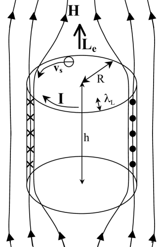
Figure 1: Superconducting cylinder of radius $R$ and height $h$ in a magnetic field. The angular momentum of the supercurrent $\vec{L}_{e}$ is parallel to the applied field $\vec{H}$. Current $I$ flows within a shell of thickness $\lambda_{L}$ near the surface, in clockwise direction as seen from the top.

The London penetration depth $\lambda_{L}$ can be measured by standard techniques lambda ; lambda2 ; lambda3 . In this paper we ask the question: for given measured values of $\lambda_{L}$ and $H$, what is the value of the superfluid velocity $v_{s}$? It cannot be inferred from Eq. (4) because $n_{s}$ is not known. $\lambda_{L}$ determines the ratio of superfluid density $n_{s}$ to effective mass $m^{*}$ through the standard relation tinkham ; londonbook ; schriefferbook

$$\frac{1}{\lambda_{L}^{2}}=\frac{4\pi n_{s}e^{2}}{m^{*}c^{2}}.$$ (5)

We assume an isotropic superconductor for simplicity. Optical optical1 ; optical2 ; optical3 as well as other experiments uemura can measure the superfluid weight $n_{s}/m^{*}$, but there are no experiments that measure $n_{s}$ nor $m^{*}$ separately. As a consequence, it is often stated that $m^{*}$ for the superfluid carriers is arbitrary and at our disposal tinkham ; degennes , for example in de Gennes’ book it is stated degennes ‘We could just as well have chosen the mass of the sun’, and in Tinkham’s book it is stated tinkham ‘In view of the experimental inaccessibility of $m^{*}$ …’.

In this paper we argue that this is not so. We point out that even though $v_{s}$ has never been experimentally measured, it can in principle be measured through Compton scattering experiments compton1 ; compton2 . Theoretically, we argue that the mass that enters in Eq. (5) is necessarily the $bare$ electron mass $m_{e}$ rather than the effective (band) mass $m^{*}$. We show that from a purely theoretical point of view Eq. (5) with $m^{*}\neq m_{e}$ is untenable. Since conventional BCS-London theory predicts that $m^{*}$ in Eq. (5) is the effective mass einzel ; einzel2 ; londonours ; scal ; misawa ; carbotte ; chak ; franz ; gross , which can be very different from the bare electron mass heavyf , this implies that conventional BCS-London theory of superconductivity is untenable. On the other hand, we point out that the alternative theory of hole superconductivity holesc predicts that $m^{*}=m_{e}$ in Eq. (5).

By measuring $v_{s}$ through Compton scattering experiments compton1 ; compton2 one would obtain $n_{s}$ from Eq. (4) and $m^{*}$ from Eq. (5),

$$m^{*}=\frac{e\lambda_{L}H}{cv_{s}},$$ (6)

hence our prediction that $m^{*}$ is necessarily $m_{e}$ can be tested experimentally.

II Superfluid velocity in the Conventional theory

In this section and in Appendix A we review the conventional arguments from which it follows that the mass in Eq. (5) is the band effective mass within BCS theory einzel ; einzel2 ; londonours ; scal ; misawa ; carbotte ; chak ; franz ; gross . In subsequent sections we will show that this conclusion is untenable in view of experimental properties of superconductors. For simplicity we consider only zero temperature. This can be extended to finite temperatures along the lines of Ref. einzel . We assume for simplicity and definiteness that any corrections to the band effective mass arising from Fermi liquid effects, electron-phonon interactions, etc, can be ignored.

We consider a simple one-band model to make our point clearly. The ground state wave function in BCS theory is given by

$$|\Psi>=\prod_{k}(\bar{u}_{k}+\bar{v}_{k}c_{k\uparrow}^{\dagger}c_{-k\downarrow}^{\dagger})|0>$$ (7)

where $k$ labels Bloch states (we omit vector labels on the $k$’s for simplicity). The mechanical momentum of a Bloch electron $\Psi_{k}(\vec{r})$ with wavevector $k$ is am

$$\vec{p}_{k}=m_{e}\vec{v}_{k}=<\Psi_{k}|\frac{\hbar}{i}\vec{\nabla}|\Psi_{k}>=m_{e}\frac{1}{\hbar}\frac{\partial\epsilon_{k}}{\partial\vec{k}}$$ (8)

where $m_{e}$ is the $bare$ electron mass and $\epsilon_{k}$ is the band energy. Note that the electron’s mechanical momentum is $not$ $\hbar\vec{k}$, nor is it $m^{*}v_{k}$. Following the semiclassical model of electron dynamics we assume that in the presence of slowly varying external fields electrons can be described by wavepackets labeled by wavevector $k$, centered at $\vec{r}$ and spread out over many lattice constants but of spatial extent much smaller that the wavelength of any applied fields, with velocity $v_{k}(\vec{r})$. The semiclassical equation of motion in the presence of an external force $\vec{F}_{ext}$ is

$$\frac{d(\hbar\vec{k})}{dt}=\vec{F}_{ext}$$ (9)

so that the time evolution of the electron mechanical momentum is, on one hand

$$\frac{d\vec{p}_{k}}{dt}=\vec{F}_{ext}+\vec{F}_{latt}$$ (10)

and on the other hand

$$\frac{d\vec{p}_{k}}{dt}=\frac{m_{e}}{\hbar^{2}}\frac{\partial^{2}\epsilon_{k}}{\partial\vec{k}\partial\vec{k}}\frac{d(\hbar\vec{k})}{dt}=\frac{m_{e}}{\hbar^{2}}\frac{\partial^{2}\epsilon_{k}}{\partial\vec{k}\partial\vec{k}}(\vec{F}_{ext}).$$ (11)

In Eq. (10), $\vec{F}_{latt}$ is the force exerted by the lattice on the electron. We assume an isotropic band and define

$$\frac{1}{m^{*}_{k}}=\frac{1}{\hbar^{2}}\frac{\partial^{2}\epsilon_{k}}{\partial k^{2}}$$ (12)

Under application of a magnetic field to the cylinder the Faraday electric field that develops within a London penetration depth of the surface is

$$\vec{E}_{F}=-\frac{\lambda_{L}}{c}\frac{\partial H}{\partial t}\hat{\theta}$$ (13)

in the azimuthal direction, exerting an external force $\vec{F}_{ext}=e\vec{E}_{F}$ on electrons, so that their mechanical momentum changes according to equation (11) as

$$\frac{d\vec{p}_{k}}{dt}=\frac{m_{e}}{m^{*}_{k}}(e\vec{E}_{F})=-\frac{m_{e}}{m^{*}_{k}}\frac{e\lambda_{L}}{c}\frac{\partial H}{\partial t}\hat{\theta}$$ (14)

and the change in mechanical momentum and velocity of the electron when the magnetic field increases from $0$ to $H$ is

$$\Delta\vec{p}_{k}=-\frac{m_{e}}{m^{*}_{k}}\frac{e\lambda_{L}}{c}H\hat{\theta}$$ (15a)

$$\Delta\vec{v}_{k}=-\frac{1}{m^{*}_{k}}\frac{e\lambda_{L}}{c}H\hat{\theta}$$ (15b)

respectively. At zero temperature the occupancy of the Bloch state with wavevector $k$ is

$$n_{k}=2|\bar{v}_{k}|^{2}=2(1-|\bar{u}_{k}|^{2})$$ (16)

where $\bar{v}_{k}$, $\bar{u}_{k}$ are the BCS amplitudes in Eq. (7), which are $1$ or $0$ except in the neighborhood of the Fermi surface. The current density that develops is then

$$\vec{J}=\frac{e}{V}\sum_{k}n_{k}(\vec{v}_{k}+\Delta\vec{v}_{k})=-\frac{1}{V}\sum_{k}n_{k}\frac{1}{m^{*}_{k}}\frac{e^{2}\lambda_{L}}{c}H\hat{\theta}$$ (17)

since the first term gives zero. Using eq. (2) yields for the penetration depth

$$\frac{1}{\lambda_{L}^{2}}=\frac{4\pi e^{2}}{c^{2}}(\frac{1}{V}\sum_{k}n_{k}\frac{1}{m^{*}_{k}}).$$ (18)

For a band that is close to empty we can assume that $m^{*}_{k}\sim m^{*}$ approximately independent of $k$ for the states for which $n_{k}\neq 0$, and Eq. (18) is

$$\frac{1}{\lambda_{L}^{2}}=\frac{4\pi n_{s}e^{2}}{m^{*}c^{2}}$$ (19)

since

$$\frac{1}{V}\sum_{k}n_{k}\frac{1}{m^{*}_{k}}=\frac{n_{s}}{m^{*}}$$ (20a)

with

$$n_{s}=\frac{1}{V}\sum_{k}n_{k}$$ (20b)

the number of superfluid carriers per unit volume. The velocity shift Eq. (15b) is independent of $k$ and given by

$$\Delta\vec{v}_{k}\equiv\vec{v}_{s}=-\frac{e\lambda_{L}}{m^{*}c}H\hat{\theta}.$$ (21a)

$$v_{s}$$ is the speed of the supercurrent carriers, and the supercurrent Eq. (17) is

$$\vec{J}=en_{s}\vec{v}_{s}.$$ (21b)

Similarly for a band that is close to full we use that

$$\sum_{all\ k}\frac{1}{m^{*}_{k}}=0$$ (22)

and defining $m^{*}=-m^{*}_{k}$, assumed independent of $k$ for the states for which $(2-n_{k})\neq 0$ we have

$$\frac{1}{V}\sum_{k}n_{k}\frac{1}{m^{*}_{k}}=\frac{1}{V}\sum_{k}(2-n_{k})\frac{1}{(-m^{*}_{k})}=\frac{n_{s}}{m^{*}}$$ (23a)

with the superfluid density now given by

$$n_{s}=\frac{1}{V}\sum_{k}(2-n_{k})$$ (23b)

so that the same expression Eq. (19) for the London penetration depth results. The velocity of the supercurrent carriers is still given by Eq. (21a), and the same expression for the supercurrent $\vec{J}=en_{s}\vec{v}_{s}$ results. These results can also be derived by using the standard linear response theory formalism as discussed in Appendix A.

The fact that we end up with the band effective mass $m^{*}$ in the expressions for the London penetration depth Eq. (19) and superfluid velocity Eq. (21a) can be traced back to the form of the BCS wavefunction Eq. (7). In particular to the fact that within BCS theory the states $k$ are the same as in the normal metal, only a slight change in occupation of those states occurs within a region $\Delta$ of the Fermi energy, with $\Delta$ the energy gap. The same results Eqs. (19) and (21a) would of course apply to a perfect conductor rather than a superconductor. This implies that if $m_{e}$ rather than $m^{*}$ has to appear in Eqs. (19) and (21a) some rather profound modification of the BCS wavefunction would be needed.

III mechanical momentum of the supercurrent

The mechanical momentum of a Bloch electron is given by Eq. (8), so when the supercurrent is generated the change in the momentum of one electron is

$$\Delta\vec{p}_{k}=m_{e}\vec{v}_{s}=-\frac{m_{e}}{m^{*}}\frac{e\lambda_{L}}{c}H\equiv\vec{p}_{mech}$$ (24)

where we used Eq. (21a) for the superfluid velocity. The mechanical momentum density per unit volume (which is zero in the absence of current) is

$$\mathcal{P}_{mech} = \frac{1}{V}\sum_{k}n_{k}\Delta p_{k}=n_{s}\Delta p_{k}=n_{s}m_{e}v_{s}$$

$$= \frac{m_{e}}{e}J=-m_{e}n_{s}\frac{e\lambda_{L}}{m^{*}c}H=-\frac{m_{e}c}{4\pi\lambda_{L}e}H$$

or alternatively

$$\mathcal{P}_{mech} = \frac{1}{V}\sum_{k}n_{k}\Delta p_{k}=\frac{m_{e}}{e}J=$$

$$= -\frac{m_{e}e\lambda_{L}}{c}H\frac{1}{V}\sum_{k}\frac{n_{k}}{m^{*}_{k}}=-\frac{m_{e}c}{4\pi\lambda_{L}e}H$$

where we have used Eqs. (19) or (18) in the last equality. Note that Eqs. (24) and (25a) apply to the particular cases where the band is close to empty or close to full, while Eq. (25b) is valid for any band filling The same results are obtained using the linear response formalism in Appendix A. Note that the mechanical momentum density is independent of the effective mass. The total angular momentum of the supercurrent for the cylinder of radius $R$ and height $h$ is the volume of the shell of thickness $\lambda_{L}$ where the supercurrent flows times the momentum density times the radius R, under the assumption that $R>>\lambda_{L}$:

$$L_{e}=(2\pi R\lambda_{L}h)\mathcal{P}_{mech}R=-\frac{m_{e}c}{2e}hR^{2}H.$$ (26)

The total mechanical angular momentum $L_{e}$ is independent of $\lambda_{L}$, $m^{*}$ and $n_{s}$. Hence from measurement of $L_{e}$ we cannot determine whether it is $m^{*}$ or $m_{e}$ that enters the equations, since $m^{*}$ does not enter in Eq. (26). $L_{e}$ is measured experimentally in the gyromagnetic effect gyro1 ; gyro2 ; gyro3 ; gyro4 and its value is found to be precisely as given by Eq. (26), which unfortunately says nothing new. It confirms however that the mechanical momentum of the electrons carrying the supercurrent is given by $m_{e}v_{s}$ and $not$ by $m^{*}v_{s}$.

IV Canonical momentum of the supercurrent

For the superconducting cylinder under consideration the relation between magnetic field and magnetic vector potential is simply

$$A=\lambda_{L}H$$ (27)

as follows from the relation $\vec{\nabla}\times\vec{A}=\vec{H}$. $\vec{A}$ points in the azimuthal direction. Eq. (27) assumes the Coulomb gauge $\vec{\nabla}\cdot\vec{A}=0$, or equivalently that $A$ is constant along the circumference of the cylinder. In terms of $\vec{A}$, the mechanical momentum of a carrier of the supercurrent is, from Eq. (24)

$$\vec{p}_{mech}=m_{e}\vec{v}_{s}=-\frac{m_{e}}{m^{*}}\frac{e}{c}\vec{A}.$$ (28)

Now the canonical momentum $\vec{p}$ that enters the Schrödinger equation for a particle of mass $m$ and charge $q$ moving with velocity $\vec{v}_{s}$ in the presence of a vector potential $\vec{A}$ is

$$\vec{p}=m\vec{v}_{s}+\frac{q}{c}\vec{A}$$ (29)

where $m\vec{v}_{s}$ is the mechanical (or ‘kinematic’) momentum, that equals the canonical momentum when $\vec{A}=0$. For a superconductor it is assumed that Eq. (29) applies with $q=2e$ and mass $m=2m^{*}$, with $m^{*}$ the effective mass tinkham ; london1948 ; laue1948 ; londonbook :

$$\vec{p}=2m^{*}\vec{v}_{s}+\frac{2e}{c}\vec{A}=\hbar\vec{\nabla}\varphi.$$ (30)

In Eq. (30), $\varphi$ is the phase of the macroscopic wavefunction $\Psi_{S}(\vec{r})$ describing the superfluid merc , given by

$$\Psi_{S}(\vec{r})=(n_{s}/2)^{1/2}e^{i\varphi(\vec{r})}.$$ (31)

The right-hand side of Eq. (30) results from applying the momentum operator $\vec{p}=(\hbar/i)\vec{\nabla}$ to $\Psi_{S}(\vec{r})$ assuming the superfluid density $n_{s}$ is uniform in space.

We next discuss the consequences of the phase equation Eq. (30) for (i) flux quantization, (ii) Meissner effect, and (iii) mechanical momentum:

(i) Flux quantization: in a superconducting ring, integration of Eq. (30) along a closed path in the interior of a ring where there is no current ($v_{s}=0$) leads to londonbook

$$\oint\hbar\vec{\nabla}\varphi\cdot\vec{dl}=nh=\frac{2e}{c}\oint\vec{A}\cdot\vec{dl}=\frac{2e}{c}\phi$$ (32)

with $n$ an integer and $\phi$ the magnetic flux, hence $\phi=n\phi_{0}$ with $\phi_{0}=hc/(2e)$ the flux quantum. This is verified experimentally fluxq1 ; fluxq2 .

(ii) Setting the canonical momentum $p=0$, as appropriate for the Meissner effect, yields for Eq. (30)

$$v_{s}=-\frac{e}{m^{*}c}A=-\frac{e\lambda_{L}}{m^{*}c}H$$ (33)

using Eq. (27), in agreement with Eq. (21a) for the speed of the Meissner current.

(iii) Setting $A=0$ in Eq. (30) should give the mechanical momentum of a pair for the canonical momentum, hence twice the mechanical momentum for one of the components of the pair:

$$p=2m^{*}v_{s}=2p_{mech}$$ (34)

hence

$$p_{mech}=m^{*}v_{s}=-\frac{e}{c}A=-\frac{e\lambda_{L}}{c}H$$ (35)

where we have used Eq. (21a) for the supercurrent velocity, or equivalently set $\vec{\nabla}\varphi=0$ in Eq. (30). However, Eq. (35) is wrong since it contradicts Eq. (24), and as a consequence it contradicts the results of the gyromagnetic experiments gyro1 ; gyro2 ; gyro3 which were shown in Sect. II to be consistent with Eq. (24), hence inconsistent with Eq. (35).

To reiterate this crucial point: to the extent that the BCS superfluid can be described by a macroscopic wavefunction $\Psi_{S}(\vec{r})$ with an amplitude and a phase as given by Eq. (31), as evidenced by multiple experiments merc , the mechanical momentum density of the supercurrent when $\vec{A}=0$ has to be given by, according to Eqs. (30), (31) and (33)

$$\mathcal{P}_{mech}=<\Psi|\frac{\hbar}{i}\vec{\nabla}|\Psi>=\frac{n_{s}}{2}\hbar\vec{\nabla}\varphi=n_{s}m^{*}\vec{v}_{s}=-\frac{n_{s}e\lambda_{L}}{c}H.$$ (36a)

Eq. (36a) would yield for the total mechanical angular momentum instead of Eq. (26), using Eq. (19) for the penetration depth

$$L_{e}=(2\pi R\lambda_{L}h)\mathcal{P}_{mech}R=-\frac{m^{*}c}{2e}hR^{2}H$$ (36b)

which disagrees with experiment gyro1 ; gyro2 ; gyro3 that establishes that the mechanical angular momentum is given by Eq. (26), i.e. Eq. (36b) but with $m_{e}$ rather than $m^{*}$, to an accuracy better than $1\%$ gyro3 (see footnote footnote ).

There is no way to ‘fix’ Eq. (30) to make it consistent with Eq. (24). If we write instead of Eq. (30)

$$\vec{p}=2m_{e}\vec{v}_{s}+\frac{2e}{c}\vec{A}=\hbar\vec{\nabla}\varphi$$ (37)

we will satisfy (i) (flux quantization) and (iii) (mechanical momentum) but obtain for (ii), i.e. setting A=0

$$v_{s}=-\frac{e}{m_{e}c}A=-\frac{e\lambda_{L}}{m_{e}c}H$$ (38)

in contradiction with Eq. (21a). Finally, if we write instead of Eq. (30)

$$\frac{m^{*}}{m_{e}}\vec{p}=2m^{*}\vec{v}_{s}+\frac{2e}{c}\vec{A}=\frac{m^{*}}{m_{e}}\hbar\vec{\nabla}\varphi$$ (39)

we will satisfy (ii) and (iii) but fail to satisfy (i), i.e. the flux quantum would depend on the ratio of bare mass to effective mass, in contradiction with experiment. Or in other words, Eq. (39) violates gauge invariance.

These considerations show that the conventional BCS theory of superconductivity applied to Bloch electrons leads to inconsistent results, in contradiction with what is generally believed einzel ; einzel2 ; londonours ; scal ; misawa ; carbotte ; chak ; franz ; gross . It is impossible to compatibilize the superfluid velocity Eq. (21a) depending on the effective (band) mass with the requirements imposed by flux quantization and gauge invariance and the vast experimental evidence in favor of a macroscopic superconducting wavefunction $\Psi_{S}(\vec{r})$ merc that has ‘phase rigidity’, so that $\vec{\nabla}{\varphi}=0$ in a simply connected sample in the presence of $\vec{A}$, which leads to the Meissner effect. In Appendix B we present these arguments in a concise alternative form leading to the same conclusion.

We propose that to resolve this inconsistency it is necessary to assume that the expression Eq. (21a) for the superfluid velocity is incorrect, and that the correct expression is

$$v_{s}=-\frac{e\lambda_{L}}{m_{e}c}H=-\frac{e}{m_{e}c}A.$$ (40)

which is consistent with Eq. (37) rather than Eq. (30) for the relation between canonical momentum and superfluid velocity. It should also be pointed out that Eq. (37) is consistent with experiments by Zimmermann and Mercereau zimm and Parker and Simmonds parker that measured the Compton wavelength of electrons in Josephson junctions, and D. Scalapino presents theoretical arguments for the validity of Eq. (37) in ref. scal2 . An experiment by Jaklevic et al jak detecting phase modulation by the superfluid velocity does not yield information to decide between Eqs. (30) and (37) without additional assumptions.

This then raises the questions: what was wrong in the straightforward derivation leading to Eq. (21a), or in the alternative equivalent derivation in Appendix A? How is Eq. (40) consistent with conventional BCS-London theory and Bloch’s theory of electrons in metals? We return to these questions in later sections.

V The London moment

The importance of the canonical momentum of superconducting electrons was already realized by F. London londonbook , before BCS and before the development of Ginzburg-Landau theory. London introduced the ‘local mean value of the momentum vector of the superelectrons’ $\vec{p}_{s}$:

$$\vec{p}_{s}=m_{e}\vec{v}_{s}+\frac{e}{c}\vec{A}=\vec{\nabla}\chi$$ (41)

with $\chi$ the ‘superpotential’, which we now would call $\hbar\varphi/2$. London deduced that the right-hand-side of Eq. (41) is the gradient of a scalar function from the Meissner effect, then proceeded to predict flux quantization from this equation londonbook . In addition, he argued that for a superconductor rotating with angular velocity $\vec{\omega}$ one has

$$\vec{v}_{s}(\vec{r})=\vec{w}\times\vec{r}$$ (42)

and a uniform magnetic field $\vec{B}$ gives rise to a magnetic vector potential

$$\vec{A}=\frac{\vec{B}\times\vec{r}}{2}.$$ (43)

Substitution of Eqs. (42) and (43) in Eq. (41) yields (for $\chi=0$ as appropriate for a simply-connected body londonbook )

$$(m_{e}\vec{\omega}+\frac{e}{2c}\vec{B})\times\vec{r}=0$$ (44)

which predicts a uniform magnetic field in the interior of a superconductor rotating with angular velocity $\vec{\omega}$

$$\vec{B}=-\frac{2m_{e}c}{e}\vec{\omega}$$ (45)

as experimentally measured hild . The fact that the experimentally measured magnetic field is given by Eq. (45) with the bare electron mass $m_{e}$ confirms that the mass in Eq. (41) has to be $m_{e}$ rather than the effective mass $m^{*}$ as in Eq. (30). Thus, the observed magnetic field of rotating superconductors provides further experimental evidence for the incorrectness of the BCS phase equation Eq. (30) that has $m^{*}$ in place of $m_{e}$.

VI The macroscopic superfluid wavefunction and phase rigidity

A large number of experiments with superconductors, particularly involving Josephson junctions and weak links, can be understood and described by the assumption that there exists a macroscopic single-particle-like wavefunction

$$\Psi_{S}(\vec{r})=(\frac{n_{s}}{2})^{1/2}e^{i\varphi(\vec{r})}$$ (46)

that describes the Cooper pair condensate merc . It is generally assumed that Eq. (46) follows from BCS theory, where the phase $\varphi$ for a spatially uniform situation is given by

$$\frac{\bar{v}_{k}}{\bar{u}_{k}}=|\frac{\bar{v}_{k}}{\bar{u}_{k}}|e^{i\varphi}$$ (47)

with $\bar{v}_{k},\bar{u}_{k}$ the amplitudes in the BCS wavefunction Eq. (7). However this has never been shown theoretically in a rigorous way rogovin .

Assuming the phase equation Eq. (30) is valid as required for the Meissner effect implies that

$$<\Psi_{S}(\vec{r})|\frac{\hbar}{i}\vec{\nabla}|\Psi_{S}(\vec{r)}>=n_{s}\hbar\vec{\nabla}\varphi=m^{*}n_{s}\vec{v}_{s}+n_{s}\frac{e}{c}\vec{A}.$$ (48)

In a simply connected superconductor the phase $\varphi$ is assumed to be uniform and not affected by the application of a vector potential $\vec{A}$. This is termed the ‘phase rigidity’ of the wavefunction. Hence the left-hand side of Eq. (48), the expectation value of the canonical momentum of the superfluid, vanishes and this implies the Meissner effect. More generally, Eq. (48) implies that superfluid flow is irrotational londonbook ; schriefferbook ; tinkham .

Now in the many-body framework of BCS theory, the canonical momentum operator $(\hbar/i)\vec{\nabla}$ in Eq. (48) corresponds to what we call the ‘paramagnetic’ momentum density operator in Appendix A, given by

$$\mathcal{\vec{P}}_{1}=\sum_{i}\frac{\hbar}{i}\vec{\nabla}_{i}$$ (49)

in first quantized form. We show in Appendix A that the expectation value of this operator (in second quantized form) with the many-body BCS wavefunction in the presence of a vector potential $\vec{A}$ is

$$<\Psi|\vec{\mathcal{P}}_{1}|\Psi>=\frac{e}{c}\frac{1}{V}\sum_{k}n_{k}(1-\frac{m_{e}}{m^{*}_{k}})\vec{A}$$ (50)

which is $not$ zero in a simply connected superconductor subject to a magnetic field. Comparing Eq. (50) with Eq. (48) we have to conclude that Eq. (48) is invalid. In other words, the generally held belief that BCS theory is consistent with ‘London rigidity’ so that the left-hand side of Eq. (48) does not change under application of a weak slowly varying magnetic field is invalid. The curl of the canonical momentum density Eq. (50) is non-zero, and therefore it cannot be said that within BCS theory the superfluid flow is irrotational, as generally assumed tinkham ; schriefferbook .

From Appendix A Eq. (A22) we deduce that within BCS theory

$$<\Psi|\vec{\mathcal{P}}_{1}|\Psi>=\frac{m_{e}}{e}\vec{J}-<\Psi|\vec{\mathcal{P}}_{2}|\Psi>$$ (51)

or equivalently using Eq. (A23)

$$\frac{e}{c}\frac{1}{V}\sum_{k}n_{k}(1-\frac{m_{e}}{m^{*}_{k}})\vec{A}=\frac{m_{e}}{e}\vec{J}+\frac{e}{c}\frac{1}{V}\sum_{k}n_{k}\vec{A}$$ (52)

Eq. (52) yields the correct current $\vec{J}$ in a simply connected geometry, where both $\vec{J}$ and $\vec{A}$ go to zero in the interior of the material. However, applied to a ring of thickness larger than the London penetration depth, it also predicts that $\vec{A}=0$ where $\vec{J}=0$, which is incorrect. We conclude that BCS theory does not predict flux quantization, and London would not have been able to infer the existence of a ‘superpotential’ londonbook ; london1948 and predict flux quantization from Eq. (41) had he known about the BCS wavefunction.

Note also we can rewrite Eq. (30) using $\vec{J}=n_{s}e\vec{v}_{s}$ as

$$<\Psi_{S}(\vec{r})|\frac{\hbar}{i}\vec{\nabla}|\Psi_{S}(\vec{r)}>=\frac{m^{*}}{e}\vec{J}+n_{s}\frac{e}{c}\vec{A}.$$ (53)

The ‘many body’ version of Eq. (53) would be within BCS theory

$$<\Psi|\mathcal{\vec{P}}_{1}|\Psi>=\frac{m^{*}}{e}\vec{J}+\frac{e}{c}\frac{1}{V}\sum_{k}n_{k}\vec{A}$$ (54)

which yields using Eq. (50)

$$\vec{J}=-\frac{e^{2}}{c}\frac{m_{e}}{m^{*}}\frac{1}{V}\sum_{k}n_{k}(\frac{1}{m^{*}_{k}})\vec{A}$$ (55)

which disagrees with the result predicted by BCS theory Eq. (A20). Therefore, the phase equation Eq. (30) is inconsistent with BCS theory.

If instead of the BCS phase equation Eq. (30) we assume that Eq. (37) is valid following zimm ; parker ; jak ; hild ; scal2 , it implies that

$$<\Psi_{S}(\vec{r})|\frac{\hbar}{i}\vec{\nabla}|\Psi_{S}(\vec{r)}>=n_{s}\hbar\vec{\nabla}\varphi=m_{e}n_{s}\vec{v}_{s}+n_{s}\frac{e}{c}\vec{A}.$$ (56)

and comparing Eq. (50) with Eq. (56) we have to conclude that Eq. (56) is invalid.

In summary, in this section we have shown in detail that the BCS formalism applied to Bloch electrons is incompatible with the existence of a macroscopic single-particle-like superfluid wavefunction $\Psi_{S}(\vec{r})$ with a well-defined macroscopic phase $\varphi(\vec{r})$ that obeys either Eq. (30) or Eq. (37).

VII kinetic energy of the supercurrent

Consideration of the kinetic energy of carriers of the supercurrent furnishes another $independent$ argument for the incorrectness of Eq. (21a) for the superfluid velocity.

The kinetic energy density of the supercurrent is given by

$$\mathcal{K}=\frac{H^{2}}{8\pi}$$ (57)

This follows from general arguments tinkham , and furthermore it is a $necessary$ condition for the existence of equilibrium between a normal and a superconducting phase when $H$ is the critical field londonh . Hence the kinetic energy per carrier is

$$\epsilon_{kin}=\frac{1}{n_{s}}\frac{H^{2}}{8\pi}$$ (58)

Replacing $H$ in terms of $v_{s}$ from Eq. (21a) yields

$$\epsilon_{kin}=\frac{1}{8\pi n_{s}}(\frac{m^{*}c}{e\lambda_{L}})^{2}v_{s}^{2}$$ (59)

and using Eq. (19) for $\lambda_{L}$ yields

$$\epsilon_{kin}=\frac{1}{2}m^{*}v_{s}^{2}.$$ (60)

Eq. (60) is generally assumed to be the correct expression for the kinetic energy of the supercurrent carriers tinkham .

However, the change in the kinetic energy of a Bloch electron when an external field is applied is given by

$$\Delta\epsilon_{kin} = <\Psi_{k+\Delta k}|-\frac{\hbar^{2}}{2m_{e}}\nabla^{2}|\Psi_{k+\Delta k}>$$

$$- <\Psi_{k}|-\frac{\hbar^{2}}{2m_{e}}\nabla^{2}|\Psi_{k}>$$

with $\Delta k=e\lambda_{L}/(\hbar c)H$. Eq. (61) is not equal to Eq. (60). In particular there is absolutely $no$ physical basis for having $m^{*}$ as prefactor in Eq. (60). $m^{*}$ describes the response of Bloch electrons to external fields but is in no way associated with the kinetic energy acquired by the electron.

To calculate the extra kinetic energy of a carrier in the supercurrent, consider the work done on a superfluid electron labeled by wavevector $k$ under the influence of a force $\vec{F}$:

$$dW_{k}=\vec{F}\cdot d\vec{x}_{k}.$$ (62)

where $d\vec{x}_{k}$ is the displacement of this wavepacket. When a magnetic field is applied, the force is the sum of the external force originating in the Faraday electric field and the force exerted by the lattice on the electron, $\vec{F}_{latt}$

$$dW_{k}=(e\vec{E}_{F}+\vec{F}_{latt})\cdot d\vec{x}_{k}$$ (63)

From the semicassical equation of motion we have

$$m_{e}\frac{d\vec{v}_{k}}{dt}=e\vec{E}_{F}+\vec{F}_{latt}$$ (64)

hence

$$dW_{k}=m_{e}\frac{d\vec{v}_{k}}{dt}\cdot d\vec{x}_{k}=m_{e}\vec{v}_{k}\cdot d\vec{v}_{k}=\frac{1}{2}m_{e}d(v_{k}^{2})$$ (65)

where we have used that for this electron

$$\frac{d\vec{x}_{k}}{dt}=\vec{v}_{k}.$$ (66)

In addition we have assumed that no work is spent in changing the potential energy of the carrier. Therefore we deduce from Eq. (65)

$$dW_{k}=d(\frac{1}{2}m_{e}v_{k}^{2})$$ (67)

The velocity change is given by $\vec{v}_{k}\rightarrow\vec{v}_{k}+\vec{v}_{s}$, hence the change in the right-hand-side of Eq. (67) when work $W_{k}$ is done on the carrier is

$$W_{k}=\frac{1}{2}m_{e}(\vec{v}_{k}+\vec{v}_{s})^{2}-\frac{1}{2}m_{e}v_{k}^{2}=m_{e}\vec{v}_{k}\cdot\vec{v}_{s}+\frac{1}{2}m_{e}v_{s}^{2}$$ (68)

The total work per unit volume is obtained by summing Eq. (68) over all states multiplied by the occupation of each state

$$W\equiv\frac{1}{V}\sum_{k}n_{k}W_{k}=n_{s}\frac{1}{2}m_{e}v_{s}^{2}$$ (69)

since the sum over the first term in Eq. (68) gives zero. Eq. (69) implies, by energy conservation, that the correct expression for the kinetic energy of a carrier in the supercurrent is

$$\epsilon_{kin}=\frac{1}{2}m_{e}v_{s}^{2}$$ (70)

rather than Eq. (60). Eq. (70) is consistent with the correct formula for the mechanical momentum Eq. (24).

Now if we compute the kinetic energy density of the supercurrent using Eq. (70) for the kinetic energy of a carrier, Eq. (21a) for the superfluid velocity, Eq. (19) for the London penetration depth, and $\mathcal{K}=n_{s}\epsilon_{kin}$, we find

$$\mathcal{K}=\frac{m_{e}}{m^{*}}\frac{H^{2}}{8\pi}$$ (71)

which disagrees with Eq. (57) and is incorrect. This shows once again that expressions (21a) for the superfluid velocity and Eq. (19) for the London penetration depth in terms of the effective mass rather than the bare electron mass are untenable.

VIII Experimental determination of the superfluid velocity

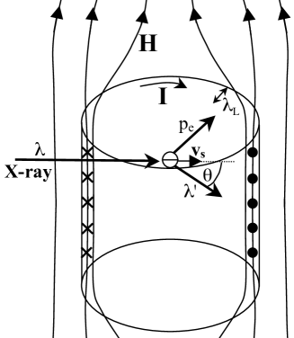
Figure 2: Compton scattering experiment on a superconducting cylinder in a magnetic field. The wavelength of the scattered X-ray for given scattering angle $\theta$ will be shifted proportionally to the superfluid velocity.

Compton scattering experiments compton1 ; compton2 offer a straightforward way, at least in principle, to measure the superfluid speed

$$v_{s}=-\frac{e\lambda_{L}}{m_{e}c}H$$ (72)

in a superconductor, as shown in Fig. 2. This is simply because in Compton scattering within the impulse approximation an individual photon is scattered by an individual electron, so the superfluid density does not play a role in determining the final state of the photon. For an X-ray incident parallel to the direction of the superfluid velocity, the difference between scattered and incident wavelengths of the photon for photon scattering angle $\theta$ is simply

$$\lambda^{\prime}-\lambda=\lambda_{c}(1\pm\frac{v_{s}}{c}(1+\frac{\lambda}{\lambda_{c}}))(1-cos\theta)$$ (73)

where the $+$/$-$ corresponds to the superelectron moving in the same / opposite direction to the incident photon. $\lambda_{c}=h/m_{e}c$ is the Compton wavelength. A typical value for the superfluid speed Eq. (72) for $\lambda_{L}=400A$ and $H=500G$ is $v_{s}=35,225cm/s$. If we take for the applied magnetic field

$$H=\frac{\hbar c}{4e\lambda_{L}^{2}}$$ (74)

which is approximately the lower critical field $H_{c1}$ tinkham1 , the superfluid speed is

$$v_{s}=\frac{\hbar}{4m_{e}\lambda_{L}}$$ (75)

and Eq. (73) takes the simple form

$$\lambda^{\prime}-\lambda=\lambda_{c}(1\pm\frac{\lambda+\lambda_{c}}{8\pi\lambda_{L}})(1-cos\theta).$$ (76a)

If instead of Eq. (72) we assume the superfluid speed is given by the BCS formula Eq. (21a) we obtain instead

$$\lambda^{\prime}-\lambda=\lambda_{c}(1\pm\frac{m_{e}}{m^{*}}\frac{\lambda+\lambda_{c}}{8\pi\lambda_{L}})(1-cos\theta).$$ (76b)

In the absence of supercurrent, the Compton scattering profile will be Doppler broadened by the velocity of the Bloch electrons. In the presence of the supercurrent the velocity of any given electron in the supercurrent will be

$$\vec{v}_{k}^{\prime}=\vec{v}_{k}+\vec{v}_{s}$$ (77)

with $\vec{v}_{k}$ its velocity in the absence of supercurrent. Thus, the Compton profile for an incident monochromatic beam will be shifted by the amount given by Eq. (72). Even though the shift is much smaller than the Doppler broadening, because it is the same for all scattering angles $\theta$ it will hopefully be detectable with currently available resolution by accumulating measurements for many angles. Thus a quantitative measurement of this Compton shift together with an independent measurement of $\lambda_{L}$ should be able to prove (or disprove) experimentally that it is the bare electron mass that enters Eq. (72) for the superfluid speed rather than the effective mass.

In addition, Compton scattering can check the prediction of the theory of hole superconductivity holesc that a spin current exists in the ground state of superconductors that flows within a London penetration depth of the surface in the absence of applied fields electrospin . In the geometry of Fig. 2, the supercarrier of spin $\vec{\sigma}$ is predicted to have azimuthal velocity

$$\vec{v}_{\sigma}=-\frac{\hbar}{4m_{e}\lambda_{L}}\vec{\sigma}\times\hat{n}-\frac{e\lambda_{L}}{m_{e}c}\hat{n}\times\vec{H}$$ (78)

where $\hat{n}$ is the outward pointing normal to the lateral surface of the cylinder. The carriers moving clockwise, with spin $\vec{\sigma}//\vec{H}$, are brought to a stop when the magnetic field reaches the value Eq. (74). For $H=0$, carriers of opposite spin flow in opposite direction with speed given by Eq. (75). Through spin-dependent Compton scattering with circularly polarized photons compton3 it will hopefully be possible to verify or disprove this prediction.

IX Discussion

In this paper we have pointed out that the speed of the supercurrent carriers in superconductors $v_{s}$, or equivalently the effective mass of carriers of the supercurrent $m^{*}$, or equivalently the density of superfluid carriers $n_{s}$, can be measured experimentally. This is contrary to the generally accepted view that only the combination $n_{s}/m^{*}$ can be directly measured, and the related generally accepted view that the superfluid velocity $\vec{v}_{s}$ is not a physical observable, only the current density $\vec{J}$ given by Eq. (21b) is. Measurement of the superfluid velocity should be able to confirm the theoretical claim discussed in this paper. However, even if the experimental accuracy required will not be attainable in the foreseeable future, it is useful to think of it as a ‘gedankenexperiment’ that can $in$ $principle$ determine what the value of the superfluid speed $v_{s}$ is. The fact that $v_{s}$ is a physical observable allows us to make the theoretical claim that BCS theory applied to Bloch electrons is internally inconsistent. In the following we summarize our arguments. In essence, we claim that BCS theory cannot describe supercurrent flow of carriers that have an effective mass $m^{*}$ in the normal state that is different from the bare electron mass $m_{e}$, and at the same time be consistent with a wide range of experimental properties of superconductors.

Before we start we should address the predictable objection of critical readers that we have ignored a large number of factors that will modify the effective mass besides the electron-ion interaction, as well as other effects not considered here: Fermi liquid effects, non-Fermi-liquid effects, electron-phonon interactions, renormalizations, multiband effects, long-range Coulomb interactions, spin-orbit interactions, magnetic interactions, Kondo physics, disorder, topological effects, relativistic effects, etc. In a real material all these effects may play a role. Nevertheless, we argue that it is a valid and useful theoretical approach to establish the inconsistency of BCS theory and band theory of solids assuming all these other effects can be ignored. While it is not $impossible$ that including some or all of these other effects could restore the consistency of BCS theory we don’t see a shred of a hint for why this would be the case. In any event it is a matter for the future to decide.

In this paper we assume electrons interact with ions as described by the standard Bloch theory of electronic energy bands in solids, disorder can be ignored, and electrons behave as independent particles except for a weak attractive interaction that leads to the BCS superconducting state below a critical temperature. We furthermore assume only one band is partially filled and hence conducts electricity, all other bands are either full or empty. For simplicity we have assumed in Appendix A that the partially filled band is the lowest band, but this restriction can be removed without altering our arguments and conclusions. We assume the system is at zero temperature.

Consider the following five points that we argue are well established:

(1) Using semiclassical transport theory (Sect. II) or equivalently the standard Kubo linear response formalism (Appendix A) it follows that within BCS theory or London theory the speed of electrons in the supercurrent is given by Eq. (21a), involving the band mass $m^{*}$ rather than the bare electron mass $m_{e}$, for the cases when a band is nearly empty or the band is nearly full. In the first case, the density $n_{s}$ of carriers carrying the supercurrent at zero temperature is the total electron density, in the second case it is the total hole density.

(2) The mechanical momentum of the carriers carrying the supercurrent is the product of the $bare$ electron mass $m_{e}$ and the superfluid velocity:

$$\vec{p}_{mech}=m_{e}\vec{v}_{s}.$$ (79)

This follows theoretically from the semiclassical treatment or equivalently from linear response theory, and is quantitatively verified by gyromagnetic effect experiments.

(3) The kinetic energy density of the supercurrent is given by

$$\mathcal{K}=\frac{H^{2}}{8\pi}.$$ (80)

This follows from general properties of the superconducting state.

(4) Superconductors exhibit many properties that establish that the superfluid is described by a single-particle-like macroscopic wavefunction $\Psi(\vec{r})$ that has a well-defined macroscopic phase $\varphi(\vec{r})$. The gradient of the phase is related to the superfluid velocity and the magnetic vector potential.

(5) For a rotating superconductor, the superfluid speed is given by Eq. (38) (the first equality) involving the bare electron mass, both in the interior region where the superfluid moves together with the body and near the surface where the superfluid lags the motion of the body londonbooklm .

We believe that the points (1)-(5) above are generally accepted, well established, experimentally proven, and true. Our claim is that BCS theory can be made to be consistent with some of those points, but not with all.

To start, we need to decide what is the equation relating the gradient of the phase, the superfluid velocity and the magnetic vector potential. We argue that Eq. (30) with the effective mass $m^{*}$ or Eq. (37) with the bare mass $m_{e}$ are the only reasonable choices. Then we argue that with either choice BCS theory is internally inconsistent. We discuss both choices in turn.

If Eq. (37) for the phase is valid, it leads to Eq. (38), the speed of the supercurrent, depending on $m_{e}$ rather than $m^{*}$. This is consistent with experiments where the entire body moves and the speed $v_{s}$ describes both the speed of the superfluid and the speed of the body hild ; zimm ; parker , however it is inconsistent when the body is at rest and a supercurrent flows. It can only be made compatible with BCS assuming the density of supercurrent carriers is neither given by the density of electrons for a nearly empty band, nor by the density of holes for a nearly full band, as shown in Appendix B. This assumption would lead to the conclusion that a superconductor and a perfect conductor respond differently to an applied magnetic field. This is inconsistent with our general understanding of superconductivity. It would also be inconsistent with BCS theory at finite temperatures, and would require that not all the Cooper pairs contribute to the supercurrent, in contradiction with BCS theory.

If instead Eq. (30) for the phase is valid, it is consistent with the Meissner effect when the phase is constant, with the superfluid velocity given by the BCS expression Eq. (21a) involving the effective mass. However, Eq. (30) requires that the mechanical momentum of electrons in the supercurrent is

$$\vec{p}_{mech}=m^{*}\vec{v}_{s}$$ (81)

and this is inconsistent with Eq. (79) for the mechanical momentum of supercurrent carriers, which follows from BCS theory $and$ agrees with experiment.

Eq. (30) for the phase is also incompatible with experiments where the entire body moves hild ; zimm ; parker . One could try to argue that Eq. (37) should be used when the superfluid moves together with the body, and Eq. (30) should be used when the superfluid moves and the body is at rest scalsuggestion . However, it is not clear then what should be used when both the body is moving and the superfluid is moving relative to the body as in the Parker-Simmonds experiment parker . Even for the rotating superconductor where the superfluid rotates together with the body in the interior, in the region within a London penetration depth of the surface there is relative motion of the supercurrent and the body to generate the interior magnetic field $\vec{B}_{i}=-(2m_{e}c/e)\vec{\omega}$ londonbooklm . Consider what happens if we apply an external magnetic field $\vec{H}=\vec{B}_{i}$ to the rotating superconductor. Electrons will respond to the Faraday electric field by changing their speed according to Eq. (21a) with $m^{*}$. However if the governing phase equation for the rotating superconductor is Eq. (37), the drift velocity before $\vec{H}$ was applied was Eq. (38) with $m_{e}$. This would imply that the drift current does not stop, which is unphysical. Physically we expect that the surface drift current will stop resulting in a uniform magnetic field $\vec{B}_{i}$ both inside and outside the superconductor.

In addition, we have shown in Sect. VI that BCS theory in the standard many-body treatment of Appendix A is incompatible with the phase rigidity that is implied by either the phase equations Eq. (30) or Eq. (37). As a consequence, BCS theory does not describe the irrotational superfluid flow required by the phase equations that is characteristic of superfluids, and it cannot predict the flux quantization for a multiply connected sample that is predicted by the phase equations and observed experimentally. The BCS wavefunction is not rigid, contrary to what the phase equations imply, rather it is modified by a long wavelength magnetic field because the perturbation induces transitions between electrons in the band responsible for superconductivity and other bands, as shown in Appendix A.

Finally and independently, we have argued that BCS theory is incompatible with the known expression for the kinetic energy density of the supercurrent Eq. (80). This expression requires that the kinetic energy of a superfluid carrier is

$$\epsilon_{kin}=\frac{1}{2}m^{*}v_{s}^{2}.$$ (82)

However this is not the kinetic energy of electrons within Bloch theory of solids under any circumstances. Using $m_{e}$ as prefactor in Eq. (82) is the correct expression for the kinetic energy of Bloch electrons under the assumption that the potential energy of carriers is independent of $v_{s}$, however this would lead to the kinetic energy density being given by Eq. (71) which is different from Eq. (80) and hence incorrect.

In summary, we have given several different independent arguments that establish that BCS theory to describe superconductivity in nature and Bloch theory of solids are mutually incompatible. The conclusion is that BCS theory in its current form is only consistent if we assume it applies to a free electron system, i.e. if $m^{*}=m_{e}$.

When F. London first introduced Eq. (30) london1948 , written in the form

$$\vec{p}_{s}=(\frac{m^{*}}{n_{s}e})\vec{J}+\frac{e}{c}\vec{A}$$ (83)

he called the left-hand-side the ‘mean momentum field of the superelectrons’ and pointed out that $\vec{\nabla}\times\vec{p}_{s}=0$ describes the Meissner effect london1948 . He assumed that $\vec{p}_{s}$ was the same canonical momentum that appears in the Schrödinger equation, $\vec{p}=(\hbar/i)\vec{\nabla}$, and pointed out that in the normal state it adopts the ‘local value’ $(e/c)\vec{A}$ in the presence of a magnetic vector potential to minimize the kinetic energy $(\vec{p}-(e/c)\vec{A})^{2}/(2m_{e})$, while in a superconductor it is prevented from doing so because of ‘rigidity’ of the wavefunction. However, he failed to notice (or to point out) that the first term on the right-hand-side of Eq. (83) is $not$ the mechanical momentum of the superelectrons if it involves $m^{*}$ rather than $m_{e}$, which converts Eq. (83) into a completely ad-hoc Ansatz with no relation to the Schrödinger equation that ultimately governs the behavior of the microscopic components of a superconductor. This may perhaps be termed the ‘original sin’ from which the contradictions discussed in this paper originated.

The findings discussed in this paper imply that the conventional BCS-London theory of superconductivity applied to electrons in energy bands of solids, as done in Refs. einzel ; einzel2 ; londonours ; scal ; misawa ; carbotte ; chak ; franz ; gross ; tinkham ; londonbook ; london1948 ; laue1948 ; schriefferbook and innumerable others, is internally inconsistent as well as inconsistent with well-established experimental properties of superconductors. This conclusion has wide-ranging implications: there are many simple metals believed to be BCS superconductors described by BCS theory spissue , and there are many normal state properties of metals that are rather well explained by Bloch’s band theory of solids am . Faced with these facts, what is the way out of this conundrum?

The problem, we propose, lies in the key BCS assumption that the states that define the BCS wavefunction Eq. (7) are the same Bloch states as in the normal state. This is properly recognized to be an assumption in Ref. einzel . The BCS amplitudes $\bar{u}_{k}$ and $\bar{v}_{k}$ in Eq. (7) tinkham differ from their values in the normal state only for values of $\epsilon_{k}$ within a region of width $\Delta$ of the Fermi energy, where $\Delta$ is the BCS energy gap. For ‘conventional’ superconductors this is certainly a tiny fraction of all the conduction electrons (or holes) in the band. Within BCS all the dramatic changes in the properties of a metal that undergoes a transition to the superconducting state result from a redistribution of the occupation of these Bloch states in the superconducting state, and all the other conduction electrons in the system, which is the vast majority, are unaffected. This is a rather remarkable statement, that condensed matter physicists have adhered to for the last 60 years. What if it is not true?

The considerations in this paper suggest that the only consistent way to interpret experiments in superconductors is to assume that electrons in the superconducting state of metals respond to applied external fields as perfectly free electrons. In other words, that carriers condensing into the superfluid state and contributing to the supercurrent become completely ‘undressed’ from electron-ion, electron-electron and electron-phonon interactions, that in the normal state dress the electron and make it respond with an effective mass $m^{*}$ rather than its bare mass $m_{e}$. This assumption consistently explains the experimental observations discussed in this paper, and it says that Eq. (37) for the phase is valid and Eq. (30) is invalid. It also explains why the work done by the external field changes only the kinetic energy and not the potential energy of superfluid carriers as assumed in Sect. VII.

We have assumed an isotropic band structure in this paper for simplicity. Of course many real solids are anisotropic. In the conventional treatment it is assumed that the effective mass is a tensor laue1948 . Here we propose instead that the mass is a scalar, the free electron mass, and anisotropies are described by a carrier density tensor, i.e. that the relation between current density and magnetic vector potential is

$$\vec{J}=-\frac{e^{2}}{m_{e}c}\overleftrightarrow{n_{s}}\cdot\vec{A}$$ (84a)

and the London kernel is

$$\overleftrightarrow{K_{L}}=\frac{4\pi e^{2}}{m_{e}c^{2}}\overleftrightarrow{n_{s}}$$ (84b)

so that along a principal axis the current is given by

$$J_{i}=-\frac{e}{m_{e}c}n_{s}^{ii}A_{i}=n_{s}^{ii}e(\vec{v}_{s})_{i}$$ (85)

with the superfluid velocity given by

$$\vec{v}_{s}=-\frac{e}{m_{e}c}\vec{A},$$ (86)

and the superfluid mechanical momentum for one carrier in a simply connected superconductor is given by

$$\vec{p}_{mech}=m_{e}\vec{v}_{s}=-\frac{e}{c}\vec{A}.$$ (87)

It follows from the discussion in this paper that whether to ascribe observed anisotropies in the London penetration depth to an effective mass tensor or to a carrier density tensor is $not$ semantics, as generally assumed. The latter is the $only$ possible choice, and it is experimentally verifiable through Compton scattering experiments.

Assuming readers agree that the points made in this paper are correct, and even before experimental confirmation by Compton scattering experiments, we suggest that the focus of theoretical research in superconductivity should switch to understanding how normal carriers in solids, governed by complicated band structures and ‘dressed’ by electron-ion, electron-electron and electron-phonon interactions, become completely ‘undressed’ from these interactions so that they respond as free electrons in the superconducting state. This was in fact the generally held view in the early days of superconductivity becker .

Within the alternative theory of hole superconductivity holesc , carriers in a nearly filled band are highly dressed in the normal state holeundr ; ehasym , and when going superconducting they expand their wavelength sm so that they no longer ‘see’ the lattice periodic potential, hence ‘undress’ from the electron-ion interaction holeelec2 and respond as free electrons. We suggest that an answer to the questions posed in this paper may be found along those lines.

Appendix A Calculation of the London kernel

In this appendix we calculate the supercurrent and the mechanical momentum density using the standard linear response formalism and show that they agree with the results obtained in Sect. II and III.

In first quantized form, the electric current density is given by $\vec{J}=(e/V)\sum_{i}\vec{v}_{i}$, with V the volume and the velocity of the i-th particle given by

$$\vec{v}_{i}=\frac{1}{m_{e}}(\vec{p}_{i}-\frac{e}{c}\vec{A}(\vec{r}_{i}))$$ (88)

with $\vec{p_{i}}$ the canonical momentum operator for the i-th particle $(\vec{p}_{i}=(\hbar/i)\vec{\nabla}_{i})$, so the current density is

$$\vec{J}=\frac{e}{m_{e}V}\sum_{i}\vec{p}_{i}-\frac{e^{2}}{m_{e}cV}\sum_{i}\vec{A}(\vec{r}_{i})\equiv\vec{J}_{1}+\vec{J}_{2}$$ (89)

with $\vec{J}_{1}$ and $\vec{J}_{2}$ the so-called paramagnetic and diamagnetic currents. We assume the vector potential $\vec{A}$ is in the Coulomb gauge, $\vec{\nabla}\cdot\vec{A}=0$. Next we rewrite $\vec{J}_{1}$ and $\vec{J}_{2}$ in second quantized form using as single particle basis the Bloch eigenfunctions of the single electron problem in the lattice ionic potential:

$$\Psi_{nk}(\vec{r})\equiv<\vec{r}|nk>$$ (90)

with $n$ labeling the n-th band and $k$ crystal momentum (we omit vector notation on k for simplicity) to obtain

$$\vec{J}_{1}=\frac{e}{m_{e}V}\sum_{n,n^{\prime},k,\sigma}c_{nk\sigma}^{\dagger}c_{n^{\prime}k\sigma}<nk|\vec{p}|n^{\prime}k>$$ (91a)

$$\vec{J}_{2}=-\frac{e^{2}}{m_{e}c}\frac{1}{V}(\sum_{nk\sigma}c_{nk\sigma}^{\dagger}c_{nk\sigma})\vec{A}$$ (91b)

assuming a uniform vector potential $\vec{A}$. The operator $c_{nk\sigma}^{\dagger}$ creates an electron with wavefunction $\Psi_{nk}(\vec{r})$ and spin $\sigma$ in the n-th band, with band energy $\epsilon_{nk}$.

We assume for simplicity an isotropic system and zero temperature. To lowest order in $\vec{A}$ the currents are given by

$$\vec{J}=\vec{J}_{1}+\vec{J}_{2}=-\frac{c}{4\pi}(K_{1}+K_{2})\vec{A}$$ (92)

with $K_{1}$ and $K_{2}$ the so-called ‘paramagnetic’ and ‘diamagnetic’ London kernels. $K_{2}$ is simply obtained by taking the expectation value of $\vec{J}_{2}$ in the BCS ground state

$$|\Psi_{G}>=\prod_{k}(\bar{u}_{k}+\bar{v}_{k}c_{0k\uparrow}^{\dagger}c_{-0k\downarrow}^{\dagger})|0>$$ (93)

where the partially filled band $n=0$ is the band giving rise to superconductivity. We assume for simplicity this is the lowest energy band, so that all other bands $n>0$ are empty at zero temperature in the absence of applied fields. To lowest order in $\vec{A}$, the diamagnetic current is simply the expectation value of $\vec{J}_{2}$ in the BCS ground state:

$$<\Psi_{G}|\vec{J}_{2}|\Psi_{G}>=-\frac{e^{2}}{m_{e}c}\frac{1}{V}\sum_{k}2|\bar{v}_{k}|^{2}\vec{A}$$ (94)

so that the diamagnetic kernel is

$$K_{2}=\frac{4\pi e^{2}}{m_{e}c^{2}}(\frac{1}{V}\sum_{k}n_{k}).$$ (95)

with $n_{k}=2|\bar{v}_{k}|^{2}$ as given by Eq. (16).

To compute the paramagnetic kernel we need the ground state wavefunction to first order in $\vec{A}$. The perturbing Hamiltonian in first quantized form is given by expanding $(\vec{p}-(e/c)\vec{A})^{2}/2m_{e}$ as

$$H_{1}=-\frac{e}{2m_{e}c}\sum_{i}(\vec{p}_{i}\cdot\vec{A}(\vec{r}_{i})+\vec{A}(\vec{r}_{i})\cdot\vec{p}_{i})$$ (96)

Its second quantized form for uniform $\vec{A}$ is

$$H_{1}=-\frac{e}{m_{e}c}\ [\sum_{nn^{\prime}k\sigma}c_{nk\sigma}^{\dagger}c_{n^{\prime}k\sigma}[<nk|\vec{p}|n^{\prime}k>]]\vec{A}$$ (97)

The wavefunction to first order in $\vec{A}$ is given by

$$|\Psi>=|\Psi_{G}>-\sum_{m}\frac{<\Psi_{m}|H_{1}|\Psi_{G}>}{E_{m}-E_{G}}|\Psi_{m}>$$ (98)

where $E_{G}$ is the energy of the BCS ground state, and $E_{m}$ the energy of the excited state $|\Psi_{m}>$. Taking the expectation value of the paramagnetic current $\vec{J}_{1}$ with this wavefunction yields

$$<\Psi|\vec{J}_{1}|\Psi>=-2Re[\sum_{m}\frac{<\Psi_{G}|\vec{J}_{1}|\Psi_{m}><\Psi_{m}|H_{1}|\Psi_{G}>}{E_{m}-E_{G}}]$$ (99)

When $H_{1}$ operates on the BCS ground state it destroys an electron in band $n^{\prime}=0$ and creates one in band $n$, either $n=0$ or $n>0$. Thus, there are two types of contributions to Eq. (A12) resulting from the states with $n=0$ and $n>0$ respectively. For the contribution from the $n=0$ states the calculation is exactly as described in Tinkham tinkham , and yields zero at zero temperature for a uniform vector potential. Thus the only contributions to Eq. (A12) come from excited states where there is one electron in a band $n>0$. Eq. (A12) then yields

$$<\Psi|\vec{J}_{1}|\Psi>=\frac{4e^{2}}{m_{e}^{2}cV}\sum_{n>0,k}|\bar{v}_{k}|^{2}\frac{<0k|p|nk><nk|p|0k>}{\epsilon_{nk}+E_{k}-\mu}\vec{A}$$ (100)

with

$$E_{k}=\sqrt{(\epsilon_{0k}-\mu)^{2}+\Delta^{2}}$$ (101)

the BCS quasiparticle excitation energy, $\mu$ the chemical potential and $\Delta$ the BCS gap. We are assuming an isotropic system and $p$ is any one component of the momentum operator.

Now the oscillator strength sum rule for Bloch electrons for isotropic energy bands yields wooten

$$\frac{2}{m_{e}^{2}}\sum_{n\neq 0}\frac{<0k|p|nk><nk|p|0k>}{\epsilon_{0k}-\epsilon_{nk}}=\frac{1}{m^{*}_{k}}-\frac{1}{m_{e}}$$ (102)

with $m^{*}_{k}$ defined by Eq. (12). The sum rule results from expanding $\epsilon_{0,k+q}$ to second order in q and using second order perturbation theory. We can use Eq. (A15) in Eq. (A13) if we approximate

$$\epsilon_{nk}+E_{k}-\mu = \epsilon_{nk}+\sqrt{(\epsilon_{0k}-\mu)^{2}+\Delta^{2}}-\mu$$ (103)

$$\sim \epsilon_{nk}-\epsilon_{0k}$$

which should be an excellent approximation when $|\bar{v}_{k}|^{2}\neq 0$. Eq. (A13) then yields

$$<\Psi|\vec{J}_{1}|\Psi>=-\frac{e^{2}}{cV}\sum_{k}2|\bar{v}_{k}|^{2}(\frac{1}{m^{*}_{k}}-\frac{1}{m_{e}})\vec{A}$$ (104)

and we obtain for the paramagnetic London kernel

$$K_{1}=\frac{4\pi e^{2}}{c^{2}}\frac{1}{V}\sum_{k}n_{k}(\frac{1}{m^{*}_{k}}-\frac{1}{m_{e}})$$ (105)

and for the total kernel

$$K=K_{1}+K_{2}=\frac{4\pi e^{2}}{c^{2}}\frac{1}{V}\sum_{k}n_{k}\frac{1}{m^{*}_{k}}$$ (106)

in agreement with Eq. (18). The total current to first order in $\vec{A}$ is

$$<\Psi|\vec{J}_{1}+\vec{J}_{2}|\Psi>=-\frac{e^{2}}{cV}\sum_{k}n_{k}(\frac{1}{m^{*}_{k}})\vec{A}$$ (107)

which agrees with Eq. (17) since $A=\lambda_{L}H$ in the cylindrical geometry under consideration.

The same formalism applies to the mechanical momentum density $\mathcal{P}_{mech}$. From Eq. (A1), the mechanical momentum of a carrier is

$$\vec{p}_{i}^{mech}=m_{e}\vec{v}_{i}=\vec{p}_{i}-\frac{e}{c}\vec{A}(\vec{r}_{i})$$ (108)

and the mechanical momentum density is

$$\vec{\mathcal{P}}_{mech}=\frac{1}{V}\sum_{i}\vec{p}_{i}-\frac{e}{cV}\sum_{i}\vec{A}(\vec{r}_{i})\equiv\vec{\mathcal{P}}_{1}+\vec{\mathcal{P}}_{2}=\frac{m_{e}}{e}(\vec{J}_{1}+\vec{J}_{2})$$ (109)

The ‘paramagnetic’ and ‘diamagnetic’ momentum densities to first order in $\vec{A}$ are

$$<\Psi|\vec{\mathcal{P}}_{1}|\Psi>=-\frac{m_{e}e}{cV}\sum_{k}n_{k}(\frac{1}{m^{*}_{k}}-\frac{1}{m_{e}})\vec{A}$$ (110a)

$$<\Psi_{G}|\vec{\mathcal{P}}_{2}|\Psi_{G}>=-\frac{e}{c}\frac{1}{V}\sum_{k}n_{k}\vec{A}$$ (110b)

and the total mechanical momentum density is

$$<\Psi|\vec{\mathcal{P}}_{mech}|\Psi>=-\frac{m_{e}e}{cV}\sum_{k}n_{k}\frac{1}{m^{*}_{k}}\vec{A}=-\frac{m_{e}n_{s}e}{m^{*}c}\vec{A}$$ (111)

in agreement with Eq. (25) since $A=\lambda_{L}H$.

Note that $\mathcal{P}_{1}$ is the canonical momentum density for the many-electron system. The fact that its $T=0$ expectation value Eq. (A23a) is non-zero to first order in $\vec{A}$ indicates that the BCS wavefunction is not ‘rigid’ with respect to magnetic perturbations, contrary to what is generally believed.

Appendix B Concise formulation of the BCS inconsistency in terms of the superfluid density

In this appendix we discuss one aspect of the inherent inconsistency of BCS theory in terms that some readers may find more appealing.

Assuming the validity of Eq. (37) scal2 ; zimm ; jak ; parker ; hild so that the mechanical momentum is correctly given by $m_{e}v_{s}$, we have for a simply connected superconductor that $\vec{\nabla}\varphi=0$ and hence

$$\vec{v}_{s}=-\frac{e}{m_{e}c}\vec{A}$$ (112)

for the velocity of Cooper pairs. Calling $n_{s}/2$ the number of Cooper pairs per unit volume, each with charge 2e, the supercurrent density is then

$$\vec{J}=n_{s}e\vec{v}_{s}=-\frac{e^{2}}{c}\frac{n_{s}}{m_{e}}\vec{A}$$ (113)

The BCS wave function is given by Eq. (7), and $m^{*}_{k}$ is defined in Eq. (12). The current density to first order in $\vec{A}$ at zero temperature is, as shown in Appendix A, Eq. (A20)

$$\vec{J}=-\frac{e^{2}}{c}\frac{1}{V}\sum_{k}2|\bar{v}_{k}|^{2}(\frac{1}{m^{*}_{k}})\vec{A}$$ (114)

which also applies to tight binding models such as the Hubbard model. Comparing Eqs. (B2) and (B3),

$$\frac{n_{s}}{m_{e}}=\frac{1}{V}\sum_{k}2|\bar{v}_{k}|^{2}(\frac{1}{m^{*}_{k}})$$ (115)

The density of electrons in the system described by the BCS wavefunction Eq. (7) is

$$n_{e}=\frac{1}{V}<\Psi|(\sum_{k\sigma}c_{k\sigma}^{\dagger}c_{k\sigma})|\Psi>=\frac{1}{V}\sum_{k}2|\bar{v}_{k}|^{2}$$ (116)

When solving for the BCS wavefunction one picks the chemical potential $\mu$ so that $n_{e}$ given by Eq. (B5) yields the density of electrons in the normal state. $\mu$ will be very close to the Fermi energy in the normal state.

For a band close to empty we will have $m^{*}_{k}\sim m^{*}$ for the occupied states independent of $k$, hence from Eqs. (B4) and (B5)

$$n_{s}=(\frac{m_{e}}{m^{*}})n_{e}$$ (117)

Similarly for a band close to full we will have $m^{*}_{k}\sim(-m^{*})$ independent of $k$ for the empty states, the density of empty states in the band is

$$n_{h}=\frac{1}{V}\sum_{k}2(1-|\bar{v}_{k}|^{2})$$ (118)

and

$$n_{s}=(\frac{m_{e}}{m^{*}})n_{h}$$ (119)

These equations are valid in the absence of disorder at zero temperature. In the presence of disorder they will remain essentially unchanged in the clean limit mars .

Eqs. (B6) and (B8) say that the number of carriers in the supercurrent, $n_{s}$, at zero temperature, in the clean limit, is not equal to the number of electrons in the Bloch or tight binding band when the band is almost empty, nor equal to the number of holes when the band is almost full. An explanation of this inconsistency has not been proposed in the scientific literature to our knowledge. It implies that a perfect conductor and a superconductor would behave differently under application of a magnetic field, which is contrary to the general understanding. Note that it resembles what has been termed the ‘condensate saga’ in the study of superfluid ${}^{4}He$ saga , the fact that the measured condensate fraction is significantly lower than the superfluid ${}^{4}He$ density platz .