Bayesian optimization under mixed constraints with a slack-variable augmented Lagrangian

Abstract

An augmented Lagrangian (AL) can convert a constrained optimization problem into a sequence of simpler (e.g., unconstrained) problems, which are then usually solved with local solvers. Recently, surrogate-based Bayesian optimization (BO) sub-solvers have been successfully deployed in the AL framework for a more global search in the presence of inequality constraints; however, a drawback was that expected improvement (EI) evaluations relied on Monte Carlo. Here we introduce an alternative slack variable AL, and show that in this formulation the EI may be evaluated with library routines. The slack variables furthermore facilitate equality as well as inequality constraints, and mixtures thereof. We show how our new slack “ALBO” compares favorably to the original. Its superiority over conventional alternatives is reinforced on several mixed constraint examples.

1 Introduction

Bayesian optimization (BO), as applied to so-called blackbox objectives, is a modernization of 1970-80s statistical response surface methodology for sequential design (Mockus et al.,, 1978; Box and Draper,, 1987; Mockus,, 1989, 1994). In BO, nonparametric (Gaussian) processes (GPs, Rasmussen and Williams,, 2006) provide flexible response surface fits. Sequential design decisions, so-called acquisitions, judiciously balance exploration and exploitation in search for global optima. For a review of GP surrogate modeling and optimization in the context of computer experiments, see Santner et al., (2003), Booker et al., (1999) and Bingham et al., (2014). For a machine learning perspective, see Brochu et al., (2010), and Boyle, (2007). Until recently, most works in these literatures have focused on unconstrained optimization.

Many interesting problems contain constraints, typically specified as equalities or inequalities:

$$\min_{x}\left\{f(x):g(x)\leq 0,h(x)=0,x\in\mathcal{B}\right\},$$ (1)

where $f:\mathbb{R}^{d}\rightarrow\mathbb{R}$ is a scalar-valued objective function, and $g:\mathbb{R}^{d}\rightarrow\mathbb{R}^{m}$ and $h:\mathbb{R}^{d}\rightarrow\mathbb{R}^{p}$ are vector-valued constraint functions taken componentwise (i.e., $g_{j}(x)\leq 0$, $j=1,\dots,m$; $h_{k}(x)=0$, and $k=1,\dots,p$). We differentiate these constraints from $\mathcal{B}\subset\mathbb{R}^{d}$, which is a known (not blackbox) set, typically containing bound constraints; here we assume that $\mathcal{B}$ is a bounded hyperrectangle.

The typical setup treats $f$, $g$, and $h$ as a “joint” blackbox, meaning that providing $x$ to a single computer code reveals $f(x)$, $g(x)$, and $h(x)$ simultaneously, often at great computational expense. A common special case treats $f(x)$ as known (e.g., linear); however, the problem is still hard when $g(x)\leq 0$ defines a nonconvex valid region. A tacit goal in this setup is to minimize the number of blackbox runs required to solve the problem, and a common meter of progress tracks the best valid value of the objective (up to a relaxing threshold on the equality constraints $h$) at increasing computational budgets (# of evaluations, $n$).

Not many algorithms target global solutions to this general, constrained blackbox optimization problem. Statistical methods are acutely few. We know of no methods from the BO literature natively accommodating equality constraints, let alone mixed (equality and inequality) ones. Schonlau et al., (1998) describe how their expected improvement (EI) heuristic can be extended to multiple inequality constraints by multiplying by an estimated probability of constraint satisfaction. Here, we call this expected feasible improvement (EFI). EFI has recently been revisited by several authors (Snoek et al.,, 2012; Gelbart et al.,, 2014; Gardner et al.,, 2014). However, the technique has pathological behavior in otherwise idealized setups (Gramacy et al.,, 2016b), which is related to a so-called “decoupled” pathology (Gelbart et al.,, 2014). Some recent information-theoretic alternatives have shown promise in the inequality constrained setting (Hernández-Lobato et al.,, 2015; Picheny,, 2014); tailored approaches have shown promise in more specialized constrained optimized setups (Gramacy and Lee,, 2011; Williams et al.,, 2010; Parr et al.,, 2012).

We remark that any problem with equality constraints can be “transformed” to inequality constraints only, by applying $h(x)\leq 0$ and $h(x)\geq 0$ simultaneously. However, the effect of such a reformulation is rather uncertain. It puts double-weight on equalities and violates certain regularity (i.e., constraint qualification (Nocedal and Wright,, 2006)) conditions. Numerical issues have been reported in empirical evaluations (Sasena,, 2002). In our own empirical work [Section 4] we find unfavorable performance.

In this paper we show how a recent technique (Gramacy et al.,, 2016a) for BO under inequality constraints is naturally enhanced to handle equality constraints, and therefore mixed ones too. The method involves converting inequality constrained problems into a sequence of simpler subproblems via the augmented Lagrangian (AL, Bertsekas,, 1982)). AL-based solvers can, under certain regularity conditions, be shown to converge to locally optimal solutions that satisfy the constraints, so long as the sub-solver converges to local solutions. By deploying modern BO on the subproblems, as opposed to the usual local solvers, the resulting meta-optimizer is able to find better, less local solutions with fewer evaluations of the expensive blackbox, compared to several classical and statistical alternatives. Here we dub that method ALBO.

To extend ALBO to equality constraints, we suggest the opposite transformation to the one described above: we convert inequality constraints into equalities by introducing slack variables. In the context of earlier work with the AL, via conventional solvers, this is rather textbook (Nocedal and Wright,, 2006, Ch. 17). Handling the inequalities in this way leads naturally to solutions for mixed constraints and, more importantly, dramatically improves the original inequality-only version. In the original (non-slack) ALBO setup, the density and distribution of an important composite random predictive quantity is not known in closed form. Except in a few particular cases (Picheny et al.,, 2016), calculating EI and related quantities under the AL required Monte Carlo integration, which means that acquisition function evaluations are computationally expensive, noisy, or both. A reformulated slack-AL version emits a composite that has a known distribution, a so-called weighted non-central Chi-square (WNCS) distribution. We show that, in that setting, EI calculations involve a simple 1-d integral via ordinary quadrature. Adding slack variables increases the input dimension of the optimization subproblems, but only artificially so. The effects of expansion can be mitigated through optimal default settings, which we provide.

The remainder of the paper is organized as follows. Section 2 outlines the components germane to the ALBO approach: AL, Bayesian surrogate modeling, and acquisition via EI. Section 3 contains the bulk of our methodological contribution, reformulating the AL with slack variables and showing how the EI metric may be calculated in closed form, along with optimal default slack settings, and open-source software. Implementation details are provided in our Appendix. Section 4 provides empirical comparisons, and Section 5 concludes.

2 A review of relevant concepts: EI and AL

2.1 Expected improvement

The canonical acquisition function in BO is expected improvement (EI, Jones et al.,, 1998). Consider a surrogate $f^{n}(x)$, trained on $n$ pairs $(x_{i},y_{i}=f(x_{i}))$ emitting Gaussian predictive equations with mean $\mu^{n}(x)$ and standard deviation $\sigma^{n}(x)$. Define $f^{n}_{\min}=\min_{i=1,\ldots,n}y_{i}$, the smallest $y$-value seen so far, and let $I(x)=\max\{0,f^{n}_{\min}-Y(x)\}$ be the improvement at $x$. $I(x)$ is largest when $Y(x)\sim f^{n}(x)$ has substantial distribution below $f^{n}_{\min}$. The expectation of $I(x)$ over $Y(x)$ has a convenient closed form, revealing balance between exploitation ($\mu^{n}(x)$ under $f^{n}_{\min}$) and exploration (large $\sigma^{n}(x)$):

$$\mathbb{E}\{I(x)\}=(f^{n}_{\min}-\mu^{n}(x))\Phi\left(\frac{f^{n}_{\min}-\mu^{n}(x)}{\sigma^{n}(x)}\right)+\sigma^{n}(x)\phi\left(\frac{f^{n}_{\min}-\mu^{n}(x)}{\sigma^{n}(x)}\right),$$ (2)

where $\Phi$ ($\phi$) is the standard normal cdf (pdf). Accurate, approximately Gaussian predictive equations are provided by many statistical models (GPs, Rasmussen and Williams,, 2006).

When the predictive equations are not Gaussian, Monte Carlo schemes—sampling $Y(x)$ variates from $f^{n}(x)$ and averaging the resulting $I(x)$ values—offer a suitable, if computationally intensive, alternative. Yet most of the theory applies only to the Gaussian case. Under certain regularity conditions (e.g., Bull,, 2011), one can show that sequential designs derived by repeating the process, generating $(n+1)$-sized designs from $n$-sized ones, contain a point $x_{i}$ whose associated $y_{i}=f(x_{i})$ is arbitrarily close to the true minimum objective value, that is, the algorithm converges.

2.2 Augmented Lagrangian framework

Although several authors have suggested extensions to EI for constraints, the BO literature has primarily focused on unconstrained problems. The range of constrained BO options was recently extended by borrowing an apparatus from the mathematical optimization literature, the augmented Lagrangian, allowing unconstrained methods to be adapted to constrained problems. The AL, as a device for solving problems with inequality constraints (no $h(x)$ in Eq. (1)), may be defined as

$$L_{A}(x;\lambda,\rho)=f(x)+\lambda^{\top}g(x)+\frac{1}{2\rho}\sum_{j=1}^{m}\max\left\{0,g_{j}(x)\right\}^{2},$$ (3)

where $\rho>0$ is a penalty parameter on constraint violation and $\lambda\in\mathbb{R}_{+}^{m}$ serves as a Lagrange multiplier. AL methods are iterative, involving a particular sequence of $(x;\lambda,\rho)$. Given the current values $\rho^{k-1}$ and $\lambda^{k-1}$, one approximately solves the subproblem

$$\min_{x}\left\{L_{A}(x;\lambda^{k-1},\rho^{k-1}):x\in\mathcal{B}\right\},$$ (4)

via a conventional (bound-constrained) solver. The parameters $(\lambda,\rho)$ are updated depending on the nature of the solution found, and the process repeats. The particulars in our setup are provided in Alg. 1; for more details see (Nocedal and Wright,, 2006, Ch. 17). Local convergence is guaranteed under relatively mild conditions involving the choice of subroutine solving (4). Loosely, all that is required is that the solver “makes progress” on the subproblem. In contexts where termination depends more upon computational budget than on a measure of convergence, as in many BO problems, that added flexibility is welcome.

0:  $\lambda^{0}\geq 0$, $\rho^{0}>0$

1:  for $k=1,2,\ldots$ do

2:     Let $x^{k}$ (approximately) solve (4)

3:     Set $\lambda_{j}^{k}=\max\left(0,\lambda_{j}^{k-1}+\frac{1}{\rho^{k-1}}g_{j}(x^{k})\right)$, $j=1,\ldots,m$

4:     If $g(x^{k})\leq 0$, set $\rho^{k}=\rho^{k-1}$; otherwise, set $\rho^{k}=\frac{1}{2}\rho^{k-1}$

5:  end for

Algorithm 1 Basic augmented Lagrangian method.

However, the AL does not typically enjoy global scope. The local minima found by the method are sensitive to initialization—of starting choices for $(\lambda^{0},\rho^{0})$ or $x^{0}$; local searches in iteration $k$ are usually started from $x^{k-1}$. However, this dependence is broken when statistical surrogates drive search for solutions to the subproblems. Independently fit GP surrogates, $f^{n}(x)$ for the objective and $g^{n}(x)=(g_{1}^{n}(x),\dots,g_{m}^{n}(x))$ for the constraints, yield predictive distributions for $Y_{f}^{n}(x)$ and $Y_{g}^{n}(x)=(Y_{g_{1}}^{n}(x),\dots,Y_{g_{m}}^{n}(x))$. Dropping the $n$ superscripts, the AL composite random variable

$$Y(x)=Y_{f}(x)+\lambda^{\top}Y_{g}(x)+\frac{1}{2\rho}\sum_{j=1}^{m}\max\{0,Y_{g_{j}}(x)\}^{2}$$ (5)

can serve as a surrogate for (3); however, it is difficult to deduce the full distribution of this variable from the components of $Y_{f}$ and $Y_{g}$, even when those are independently Gaussian. While its mean is available in closed form, EI requires Monte Carlo.

3 A novel formulation involving slack variables

An equivalent formulation of (1) involves introducing slack variables, $s_{j}$, for $j=1,\dots,m$ (i.e., one for each inequality constraint $g_{j}(x)$), and converting the mixed constraint problem (1) into one with only equality constraints (plus bound constraints for $s_{j}$):

$$g_{j}(x)-s_{j}=0,\quad s_{j}\in\mathbb{R}_{+},\quad\text{for }j=1,\dots,m.$$ (6)

The input dimension of the problem is increased from $d$ to $d+m$ with the introduction of the $m$ (positive) slack “inputs” $s$.

Reducing a mixed constraint problem to one involving only equality and bound constraints is valuable insofar as one has good solvers for those problems. Indeed, the AL method is an attractive option here, but some adaptation is required. Suppose, for the moment, that the original problem (1) has no equality constraints (i.e., $p=0$). In this case, a slack variable-based AL method is readily available—as an alternative to the one described in Section 2.2. Although we frame it as an “alternative”, some in the mathematical optimization community would describe this as the standard version (see, e.g., Nocedal and Wright,, 2006, Ch. 17). The AL for this setup is given as follows:

$$L_{A}(x,s;\lambda_{g},\rho)=f(x)+\lambda^{\top}\left(g(x)\!+\!s\right)+\frac{1}{2\rho}\sum_{j=1}^{m}\left(g_{j}(x)\!+\!s_{j}\right)^{2}.$$ (7)

This formulation is more convenient than (3) because the “max” is missing, but the extra slack variables mean solving a higher ($d+m$) dimensional subproblem compared to (4). In Section 3.3 we address this issue, and further detail adjustments to Alg. 1 for the slack variable case.

The AL can be expanded to handle equality (and thereby mixed constraints) as follows:

$$L_{A}(x,s;\lambda_{g},\lambda_{h},\rho)=f(x)+\lambda_{g}^{\top}\left(g(x)\!+\!s\right)+\lambda_{h}^{\top}h(x)+\frac{1}{2\rho}\!\left[\sum_{j=1}^{m}\left(g_{j}(x)\!+\!s_{j}\right)^{2}+\sum_{k=1}^{p}h_{k}(x)^{2}\right]\!.$$ (8)

Defining $c(x):=\left[g(x)^{\top},h(x)^{\top}\right]^{\top}\!\!$, $\lambda:=\left[\lambda_{g}^{\top},\lambda_{h}^{\top}\right]^{\top}\!\!$, and enlarging the dimension of $s$ with the understanding that $s_{m+1}=\cdots=s_{m+p}=0$, leads to a streamlined AL for mixed constraints

$$L_{A}(x,s;\lambda,\rho)=f(x)+\lambda^{\top}\left(c(x)+s\right)+\frac{1}{2\rho}\sum_{j=1}^{m+p}\left(c_{j}(x)+s_{j}\right)^{2},$$ (9)

with $\lambda\in\mathbb{R}^{m+p}$. A non-slack AL formulation (3) may be written analogously as

$$L_{A}(x;\lambda_{g},\lambda_{h},\rho)=f(x)+\lambda_{g}^{\top}g(x)+\lambda_{h}^{\top}h(x)+\frac{1}{2\rho}\left[\sum_{j=1}^{m}\max\left\{0,g_{j}(x)\right\}^{2}+\sum_{k=1}^{p}h_{k}(x)^{2}\right],$$

with $\lambda_{g}\in\mathbb{R}_{+}^{m}$ and $\lambda_{h}\in\mathbb{R}^{p}$. Eq. (9), by contrast, is easier to work with because it is a smooth quadratic in the objective ($f$) and constraints ($c$). In what follows, we show that (9) facilitates calculation of important quantities like EI, in the GP-based BO framework, via a library routine. So slack variables not only facilitate mixed constraints in a unified framework, they also lead to a more efficient handling of the original inequality (only) constrained problem.

3.1 Distribution of the slack-AL composite

If $Y_{f}$ and $Y_{c_{1}},\dots,Y_{c_{m+p}}$ represent random predictive variables from ${m+p}+1$ surrogates fitted to $n$ realized objective and constraint evaluations, then the analogous slack-AL random variable is

$$Y(x,s)=Y_{f}(x)+\sum_{j=1}^{m+p}\lambda_{j}(Y_{c_{j}}(x)+s_{j})+\frac{1}{2\rho}\sum_{j=1}^{m+p}(Y_{c_{j}}(x)+s_{j})^{2}.$$ (10)

As in the original AL formulation, the mean of this RV has a simple closed form in terms of the means and variances of the surrogates, regardless of the form of predictive distribution. In the conditionally Gaussian case, we can derive the full distribution of the slack-AL variate (10) in closed form. Toward that aim, we re-develop the composite $Y$ as follows:

$$Y(x,s) =Y_{f}(x)+\sum_{j=1}^{m+p}\lambda_{j}s_{j}+\frac{1}{2\rho}\sum_{j=1}^{m+p}s_{j}^{2}+\frac{1}{2\rho}\sum_{j=1}^{m+p}\left[2\lambda_{j}\rho Y_{c_{j}}(x)+2s_{j}Y_{c_{j}}(x)+Y_{c_{j}}(x)^{2}\right]$$

$$=Y_{f}(x)+\sum_{j=1}^{m+p}\lambda_{j}s_{j}+\frac{1}{2\rho}\sum_{j=1}^{m+p}s_{j}^{2}+\frac{1}{2\rho}\sum_{j=1}^{m+p}\left[\left(\alpha_{j}+Y_{c_{j}}(x)\right)^{2}-\alpha_{j}^{2}\right],$$

with $$\alpha_{j}=\lambda_{j}\rho+s_{j} Y(x,s)$$. Now decompose the into a sum of three quantities:

$$Y(x,s) =Y_{f}(x)+r(s)+\frac{1}{2\rho}W(x,s),\quad\mbox{with}$$ (11)

$$r(s) =\sum_{j=1}^{m+p}\lambda_{j}s_{j}+\frac{1}{2\rho}\sum_{j=1}^{m+p}s_{j}^{2}-\frac{1}{2\rho}\sum_{j=1}^{m+p}\alpha_{j}^{2}\quad\mbox{and}\quad W(x,s)=\sum_{j=1}^{m+p}\left(\alpha_{j}+Y_{c_{j}}(x)\right)^{2}.$$

Using $Y_{c_{j}}\sim\mathcal{N}\left(\mu_{c_{j}}(x),\sigma^{2}_{c_{j}}(x)\right)$, i.e., leveraging Gaussianity, $W$ can be written as

$$W(x,s)=\sum_{j=1}^{m+p}\sigma^{2}_{c_{j}}(x)X_{j}(x,s),\quad\mbox{with }X_{j}(x,s)\sim\chi^{2}\left(\mathrm{dof}\!=\!1,\delta\!=\!\left(\frac{\mu_{c_{j}}(x)+\alpha_{j}}{\sigma_{c_{j}}(x)}\right)^{2}\right).\hfill$$ (12)

The line above is the expression of a weighted sum of non-central chi-square (WSNC) variates. Each of the ${m+p}$ variates involves a unit degrees-of-freedom (dof) parameter, and a non-centrality parameter $\delta$. A number of efficient methods exist for evaluating the density, distribution, and quantile functions of WSNC random variables (e.g., Davies,, 1980; Duchesne and Lafaye de Micheaux,, 2010). The R packages CompQuadForm (Lafaye de Micheaux,, 2013) and sadists (Pav,, 2015) provide library implementations. Details and code are provided in Appendix C.

Some constrained optimization problems involve an a priori known objective $f(x)$. In that case, referring back to (11), we are done: the distribution of $Y(x,s)$ is WSNC (as in (12)) shifted by a known quantity $f(x)+r(s)$, determined by particular choices of inputs $x$ and slacks $s$. When $Y_{f}(x)$ is conditionally Gaussian we have that $\tilde{W}(x,s)=Y_{f}(x)+\frac{1}{2\rho}W(x,s)$ is the weighted sum of a Gaussian and WNCS variates, a problem that is again well-studied. The same methods cited above are easily augmented to handle that case—see Appendix C.

3.2 Slack-AL expected improvement

Evaluating EI at candidate $(x,s)$ locations under the AL-composite involves working with $\mathrm{EI}(x,s)=\mathbb{E}\left[\left(y_{\min}^{n}-Y(x,s)\right)\mathbb{I}_{\{Y(x,s)\leq y_{\min}^{n}\}}\right]$, given the current minimum $y^{n}_{\min}$ of the AL over all $n$ runs. When $f(x)$ is known, let $w^{n}_{\min}(x,s)=2\rho\left(y^{n}_{\min}-f(x)-r(s)\right)$ absorb all of the non-random quantities involved in the EI calculation. Then, with $D_{W}(\cdot;x,s)$ denoting the distribution of $W(x,s)$,

$$\mathrm{EI}(x,s) = \frac{1}{2\rho}\mathbb{E}\left[\left(w^{n}_{\min}(x,s)-W(x,s)\right)\mathbb{I}_{W(x,s)\leq w_{\min}(x,s)}\right]$$ (13)

$$= \frac{1}{2\rho}\int_{-\infty}^{w^{n}_{\min}(x,s)}D_{W}(t;x,s)dt=\frac{1}{2\rho}\int_{0}^{w^{n}_{\min}(x,s)}D_{W}(t;x,s)dt$$

if $w^{n}_{\min}(x,s)\geq 0$ and zero otherwise. That is, the EI boils down to integrating the distribution function of $W(x,s)$ between 0 (since $W$ is positive) and $w^{n}_{\min}(x,s)$. This is a one-dimensional definite integral that is easy to approximate via quadrature; details are in Appendix C. Since $W(x,s)$ is quadratic in the $Y_{c}(x)$ values, it is often the case, especially for smaller $\rho$-values in later AL iterations, that $D_{W}(t;x,s)$ is zero over most of $[0,w^{n}_{\min}(x,s)]$, simplifying the numerical integration. However, this has deleterious impacts on search over $(x,s)$. We discuss a useful adaptation for that case in Appendix B.2.

When $f(x)$ is unknown and $Y_{f}(x)$ is conditionally normal, let $\tilde{w}^{n}_{\min}(s)=2\rho\left(y^{n}_{\min}-r(s)\right)$. Then,

$$\mathrm{EI}(x,s)=\frac{1}{2\rho}\mathbb{E}\left[\left(\tilde{w}^{n}_{\min}(s)-\tilde{W}(x,s)\right)\mathbb{I}_{\tilde{W}(x,s)\leq\tilde{w}^{n}_{\min}(s)}\right]=\frac{1}{2\rho}\int_{-\infty}^{\tilde{w}^{n}_{\min}(s)}D_{\tilde{W}}(t;x,s)dt.$$

Here the lower bound of the definite integral cannot be zero since $Y_{f}(x)$ may be negative, and thus $\tilde{W}(x,s)$ may have non-zero distribution for negative $t$-values. This presents some challenges when it comes to numerical integration via quadrature, although many library functions allow indefinite bounds. We obtain better performance by supplying a conservative finite lower bound, for example three standard deviations in $Y_{f}(x)$, in units of the penalty ($2\rho$), below zero: $6\rho\sigma_{f}(x)$. Detailed example implementations are provided Appendix C.

3.3 AL updates, optimal slacks, and other implementation notes

The new slack-AL method is completed by describing when the subproblem (9) is deemed to be “solved” (step 2 in Alg. 1), how $\lambda$ and $\rho$ updated (steps 3–4). We terminate the BO search sub-solver after a single iteration as this matches with the spirit of EI-based search, whose choice of next location can be shown to be optimal, in a certain sense, if it is the final point being selected (Bull,, 2011). It also meshes well with an updating scheme analogous to that in steps 3–4: updating only when no actual improvement (in terms of constraint violation) is realized by that choice. For those updates, the analog for the mixed constraint setup is

step 2: Let $(x^{k},s^{k})$ approx. solve $\min_{x,s}\!\left\{L_{A}(x,s;\lambda^{k-1},\rho^{k-1}):(x,s_{1:m})\in\tilde{\mathcal{B}}\right\}$
step 3: $\lambda_{j}^{k}=\lambda_{j}^{k-1}+\frac{1}{\rho^{k-1}}(c_{j}(x^{k})+s_{j}^{k})$, for $j=1,\dots,m+p$
step 4: If $c_{1:m}(x^{k})\leq 0$ and $|c_{m+1:m+p}(x^{k})|\leq\epsilon$, set $\rho^{k}\!\!=\!\!\rho^{k-1}$; else $\rho^{k}\!=\!\frac{1}{2}\rho^{k-1}$

Above, step 3 is the same as in Alg. 1 except without the “max”, and with slacks augmenting the constraint values. The “if” statement in step 4 checks for validity at $x^{k}$, deploying a threshold $\epsilon\geq 0$ on equality constraints; further discussion of the threshold $\epsilon$ is deferred to Section 4, where we discuss progress metrics under mixed constraints. If validity holds at $(x^{k},s^{k})$, the current AL iteration is deemed to have “made progress” and the penalty remains unchanged; otherwise it is doubled. An alternate formulation may check $|c_{1:m}(x^{k})+s_{1:m}^{k}|\leq\epsilon$. We find that the version in step 4, above, is cleaner because it limits sensitivity to the choice of threshold $\epsilon$. In Appendix B.1 recommend initial $(\lambda^{0},\rho^{0})$ values which are analogous to the original, non-slack AL settings.

Optimal choice of slacks: The biggest difference between the original AL (3) and slack-AL (9) is that the latter requires searching over both $x$ and $s$, whereas the former involves only $x$-values. In what follows we show that there are automatic choices for the $s$-values as a function of the corresponding $x$’s, keeping the search space $d$-dimensional, rather than $d+m$.

For an observed $c_{j}(x)$ value, associated slack variables minimizing the AL (9) can be obtained analytically. Using the form of (11), observe that $\min_{s\in\mathbb{R}_{+}^{m}}y(x,s)$ is equivalent to $\min_{s\in\mathbb{R}_{+}^{m}}\sum_{j=1}^{m}2\lambda_{j}\rho s_{j}+s_{j}^{2}+2s_{j}c_{j}(x)$. For fixed $x$, this is strictly convex in $s$. Therefore, its unconstrained minimum can only be its stationary point, which satisfies $0=2\lambda_{j}\rho+2s_{j}^{*}(x)+2c_{j}(x)$, for $j=1,\dots,m$. Accounting for the nonnegativity constraint, we obtain the following optimal slack as a function of $x$:

$$s_{j}^{*}(x)=\max\left\{0,-\lambda_{j}\rho-c_{j}(x)\right\},\qquad j=1,\dots,m.$$ (14)

Above we write $s^{*}$ as a function of $x$ to convey that $x$ remains a “free” quantity in $y(x,s^{*}(x))$. Recall that slacks on equality constraints are zero, $s_{k}(x)=0$, $k=m+1,\dots,m+p$, for all $x$.

In the blackbox $c(x)$ setting, $y(x,s^{*}(x))$ is only directly accessible at the data locations $x_{i}$. At other $x$-values, however, the surrogates provide a useful approximation. When $Y_{c}(x)$ is (approximately) Gaussian it is straightforward to show that the optimal setting of the slack variables, solving $\min_{s\in\mathbb{R}_{+}^{m}}\mathbb{E}[Y(x,s)]$, are $s_{j}^{*}(x)=\max\{0,-\lambda_{j}\rho-\mu_{c_{j}}(x)\}$, i.e., the same as (14) with a prediction $\mu_{c_{j}}(x)$ for $Y_{c_{j}}(x)$ unknown $c_{j}(x)$ value. Again, slacks on the equality constraints are set to zero.

Other criteria can be used to choose slack variables. Instead of minimizing the mean of the composite, one could maximize the EI. In Appendix A we explain how this is of dubious practical value. Compared to the settings described above, searching over EI is both more computationally intensive and provides near identical results in practice.

Implementation notes: Code supporting all methods in this manuscript is provided in two open-source R packages: laGP (Gramacy,, 2015) and DiceOptim (Ginsbourger et al.,, 2015), both on CRAN (R Development Core Team,, 2004). Implementation details vary somewhat across those packages, due primarily to particulars of their surrogate modeling capability and how they search the EI surface. For example, laGP can accommodate a smaller initial design size because it learns fewer parameters (i.e., has fewer degrees of freedom). DiceOptim uses a multi-start search procedure for EI, whereas laGP deploys a random candidate grid, which may optionally be “finished” with an L-BFGS-B search. Nevertheless, their qualitative behavior exhibits strong similarity. Both packages also implement the original AL scheme (i.e., without slack variables) updated (8) for mixed constraints. Further details are provided in Appendix B.2.

4 Empirical comparison

Here we describe three test problems, each mixing challenging elements from traditional unconstrained blackbox optimization benchmarks, but in a constrained optimization format. We run our optimizers on these problems 100 times under random initializations. In the case of our GP surrogate comparators, this initialization involves choosing random space-filling designs. Our primary means of comparison is an averaged (over the 100 runs) measure of progress defined by the best valid value of the objective for increasing budgets (number of evaluations of the blackbox), $n$.

In the presence of equality constraints it is necessary to relax this definition somewhat, as the valid set may be of measure zero. In such cases we choose a tolerance $\epsilon\geq 0$ and declare a solution to be “valid” when inequality constraints are all valid, and when $|h_{k}(x)|\leq\epsilon$ for all $k=1,\dots,p$. In our figures we choose $\epsilon=10^{-2}$; however, the results are similar under stronger thresholds, with a higher variability over initializations. As finding a valid solution is, in itself, sometimes a difficult task, we additionally report the proportion of runs that find valid and optimal solutions as a function of budget, $n$, for problems with equality (and mixed) constraints.

4.1 An inequality constrained problem

We first revisit the “toy” problem from Gramacy et al., (2016a), having a 2-d input space limited to the unit cube, a (known) linear objective, with sinusoidal and quadratic inequality constraints (henceforth LSQ problem; see the Appendix D for details). Figure 1 shows progress over repeated solves with a maximum budget of 40 blackbox evaluations.

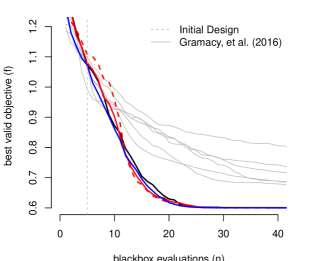
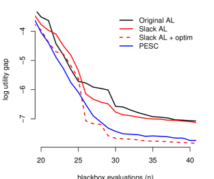
Figure 1: Results on the LSQ problem with initial designs of size $n=10$. The left panel shows the best valid value of the objective over the first 40 evaluations, whereas the right shows the $\log$ utility-gap for the second 20 evaluations. The solid gray lines show comparators from Gramacy et al., (2016a).

The left-hand plot in Figure 1 tracks the average best valid value of the objective found over the iterations, using the progress metric described above. Random initial designs of size $n=5$ were used, as indicated by the vertical-dashed gray line. The solid gray lines are extracted from a similar plot from Gramacy et al., (2016a), containing both AL-based comparators, and several from the derivative-free optimization and BO literatures. The details are omitted here. Our new ALBO comparators are shown in thicker colored lines; the solid black line is the original AL(BO)-EI comparator, under a revised (compared to (Gramacy et al.,, 2016a)) initialization and updating scheme. The two red lines are variations on the slack-AL algorithm under EI: with (dashed) and without (solid) L-BFGS-B optimizing EI acquisition at each iteration. Finally, the blue line is PESC Hernández-Lobato et al., (2015), using the Python library available at https://github.com/HIPS/Spearmint/tree/PESC. The take-home message from the plot is that all four new methods outperform those considered by the original ALBO paper Gramacy et al., (2016a).

Focusing on the new comparators only, observe that their progress is nearly statistically equivalent during the first 20 iterations. At iteration 10, for example, the ordering from best to worst is PESC (0.861), Slack-AL (0.902), Orig-AL (0.942), and Slack-AL+optim (0.957). Combining the 100 repetitions of each run, only the best (PESC) versus worst (Slack-AL+optim) is statistically significant in a one-sided $t$-test, with a $p$-value of 0.0011. Apparently, aggressively optimizing the EI in the slack formulation in early iterations hurts more than it helps. The situation is more nuanced, however, for later iterations. At iteration 30, for example, the ordering is Slack-AL+optim (0.6002), PESC (0.6004), Slack-AL (0.6010), and Orig-AL (0.689). Although the numbers are more tightly grouped, only the first two (Slack-AL+optim and PESC), both leveraging L-BFGS-B subroutines, are statistically equivalent. In particular, both Slack-AL variants outperform the original AL with $p$-values less than $2.2e^{-16}$. This discrepancy is more easily visualized in the left of the figure with a so-called “utility-gap” log plot (Hernández-Lobato et al.,, 2015), which tracks the log difference between the theoretical best valid value and those found by search.

4.2 Mixed inequality and equality constrained problems

Next consider a problem in four input dimensions with a (known) linear objective and two constraints, one inequality and one equality. The inequality constraint is the so-called “Ackley” function in $d=4$ input dimensions. The equality constraint follows the so-called “Hartman 4-dimensional function”. Appendix D provides a full mathematical specification.

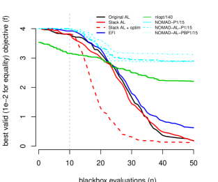
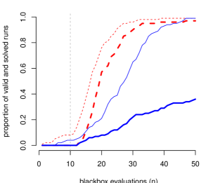
Figure 2: Results on the Linear-Hartman-Ackley mixed constraint problem. The left panel shows a progress comparison based on laGP code with initial designs of size $n=10$. The $x$-scale has been divided by 140 for the nlopt comparator. A value of four indicates that no valid solution has been found. The right panel shows the proportion of valid (thin lines) and optimal (thick lines) solutions for the EFI and “Slack AL + optim” comparators.

Figure 2 shows two views into progress on this problem. Since it involves mixed constraints, comparators from the BO literature are scarce. Our EFI implementation deploys the $(-h,h)$ heuristic mentioned in the introduction. As representatives from the nonlinear optimization literature we include nlopt (Johnson,, 2014) and three adapted NOMAD (Le Digabel,, 2011) comparators, which are detailed in Appendix B.3. In the left-hand plot we can see that our new ALBO comparators are the clear winner, with an L-BFGS-B optimized EI search under the slack-variable AL implementation performing exceptionally well. The nlopt and NOMAD comparators are particularly poor. We allowed those to run up to 7000 and 1000 iterations, respectively, and in the plot we scaled the $x$-axis (i.e., $n$) to put them on the same scale as the others. The right-hand plot provides a view into the distribution of two key aspects of performance over the MC repetitions. Observe that “Slack AL + optim” finds valid values quickly, and optimal values not much later. Our adapted EFI is particularly slow at converging to optimal (valid) solutions.

Our final problem involves two input dimensions, an unknown objective function (i.e., one that must be modeled with a GP), one inequality constraint and two equality constraints. The objective is a centered and re-scaled version of the “Goldstein–Price” function. The inequality constraint is the sinusoidal constraint from the LSQ problem [Section 4.1]. The first equality constraint is a centered “Branin” function, the second equality constraint is taken from Parr et al., (2012) (henceforth GBSP problem). Appendix D contains a full mathematical specification.

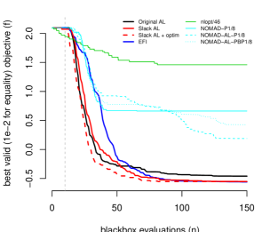
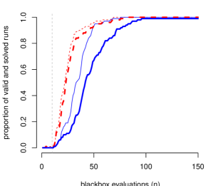
Figure 3: Results on the GBSP problem. See Figure 2 caption.

Figure 3 shows our results on this problem. Observe (left panel) that the original ALBO comparator makes rapid progress at first, but dramatically slows for later iterations. The other ALBO comparators, including EFI, converge much more reliably, with the “Slack AL + optim” comparator leading in both stages (early progress and ultimate convergence). Again, nlopt and NOMAD are poor, however note that their relative comparison is reversed; again, we scaled the $x$-axis to view these on a similar scale as the others. The right panel shows the proportion of valid and optimal solutions for “Slack AL + optim” and EFI. Notice that the AL method finds an optimal solution almost as quickly as it finds a valid one—both substantially faster than EFI.

5 Discussion

The augmented Lagrangian (AL) is an established apparatus from the mathematical optimization literature, enabling unconstrained or bound-constrained optimizers to be deployed in settings with constraints. Recent work involving Bayesian optimization within the AL framework (ALBO) has shown great promise, especially toward obtaining global solutions under constraints. However, those methods were deficient in at least two respects. One is that only inequality constraints could be supported. Another was that evaluating the acquisition function, combining predictive mean and variance information via EI, required Monte Carlo approximation. In this paper we showed that both drawbacks could be addressed via a slack-variable reformulation of the AL. Our method supports inequality, equality, and mixed constraints, and to our knowledge this updated ALBO procedure is unique in the BO literature in its applicability to the general mixed constraints problem (1). We showed that the slack ALBO method outperforms modern alternatives in several challenging constrained optimization problems.

We conclude by remarking on a potential drawback: we have found in some cases that our slack variable approach is a double-edged sword, especially when the unknown slacks are chosen in a default manner, i.e., $s^{*}(x)$ as in Section 3.3. Those choices utilize the surrogate(s) of the constraints, particularly the posterior mean, which means that those surrogates are relied upon more heavily than in the original (non-slack) AL context. Consequently, if the problem at hand matches the surrogate modeling (i.e., Gaussian process) assumptions well, then by a leveraging argument we can expect the slack method to do better than the original. However, if the assumptions are a mismatch, then one can expect them to be worse. The motivating “Lockwood” problem from Gramacy et al., (2016a) had a constraint surface that was kinked at its boundary $\{x\in\mathbb{R}^{d}:c(x)=0\}$, which obviously violates the smoothness assumptions of typical GP surrogates. We were therefore not surprised to find poorer performance in our slack method compared to the original.

Acknowledgments

We are grateful to Mickael Binois for comments on early drafts. RBG is grateful for partial support from National Science Foundation grant DMS-1521702. The work of SMW is supported by the U.S. Department of Energy, Office of Science, Office of Advanced Scientific Computing Research under Contract No. DE-AC02-06CH11357. The work of SLD is supported by the Natural Sciences and Engineering Research Council of Canada grant 418250.

Appendix A Optimal and default slack variables

This continues the discussion from Section 3.3, which suggests choosing slack variables by minimizing the slack-AL. One alternative is to maximize the EI. Recall that EI mixes data quantities (at the $x_{i}$) and predictive quantities at candidate locations $(x,s)$ via the improvement $I(x,y)=\max(0,y_{\min}^{n}-Y(x,s))$, the former coming from $y_{\min}^{n}=\min(y_{1},\dots,y_{n})$, where $y_{i}=y(x_{i},s)$. If one seeks improvement over the lowest possible $y_{\min}^{n}$, then the optimal $s$-values to pair with the $x_{i}$s are given in Eq. (14): use $y_{i}=y(x_{i},s^{*}(x_{i}))$. Choosing slacks for candidate $(x,s)$ locations is more challenging. Solving $\max_{s\in\mathbb{R}_{+}^{m}}\mathrm{EI}(x,s)$ for a fixed $x$ is equivalent to solving $\max_{s\in\mathbb{R}_{+}^{m}}\mathbb{E}\{Y(x,s)\mathbb{I}_{Y(x,s)\leq y_{\min}}\}$, for which a closed-form solution remains elusive. Numerical methods are an option; however, we have not discovered any advantage over the simpler $\min_{s\in\mathbb{R}_{+}^{m}}\mathbb{E}\{Y(x,s)\}$-based settings described above. Empirically, we find that the two criteria either yield identical $s^{*}_{j}(x)$-values, or ones that are nearly so.

As an illustration, we consider a 2-d problem with a linear objective and two inequality constraints (see the LSQ problem in Section D, Eq. (16), below). We focus here on a “static” situation, where a 9-point grid defines the set of observations. $f_{1}$ is treated as a known function and two GP models are fitted to $c_{1}$ and $c_{2}$. The AL parameters are set to $\rho=1/16$ and $\lambda=[1,1]$.

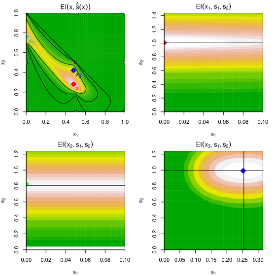
Figure 4: Illustration of the influence of the slack variables. The top left figure shows EI as a function of $x$, when the slack variables are chosen as $\hat{s}$. The three other figures show the EI metric as a function of the slack variables for three different $x$-values (at locations shown in the top left graph). The horizontal and vertical lines show the $s^{*}$-values, and the points show the optimal values.

The top-left panel of Figure 4 shows the EI surface (computed on a 2-d grid), when $s_{j}^{*}(x)=\max\left(0,-\lambda_{j}\rho-\mu_{j}(x)\right)$ is used for each grid element $x$. The shape of the contours is typical of EI, with a plateau of zero values and two local maxima. The remaining panels show the value of the EI metric for each of the three $x$-values shown in the top-left panel. These are computed on a 2-d grid in $s$ space. Despite its complex formulation (13), on this example EI is apparently unimodal with respect to $s_{1}$ and $s_{2}$. Moreover, the optimal values (computed from the grid used to plot the image) coincide (up to numerical error) with the associated $s^{*}$ values, plotted as diamonds matching the color in the top-left plot.

Appendix B Implementation notes

B.1 Initializing the AL parameters in the slack setup

To initialize $(\lambda^{0},\rho^{0})$, we update the settings suggested in Gramacy et al., (2016b)—balancing the scales of objective and constraint in the AL on the initial design of size $n_{0}$—to our new mixed constraint context. Let $v(x)$ be a logical vector of length $m+p$ recording the validity of $x$ in a zero-slack setting. That is, let $v_{j}(x)=1$ if $c_{j}(x)\leq 0$, for $j=1,\dots,p$, and $v_{j}(x)=1$ if $|c_{j}(x)|\leq\epsilon$, for $j=p+1,\dots,m$; otherwise let $v_{j}(x)=0$. Then, take

$$\rho^{0}=\frac{\min_{i=1,\dots,n_{0}}\{\sum_{j=1}^{m+p}c_{j}(x_{i})^{2}:\exists j,v_{j}(x_{i})=0\;\}}{2\min_{i=1,\dots,n_{0}}\{f(x_{i}):\forall j,v_{j}(x_{i})=1\}},$$

and $\lambda^{0}=0$. The denominator above is not defined if the initial design has no valid values (i.e., if there is no $x_{i}$ with $v_{j}(x_{i})=1$ for all $j$). When that happens we use the median of $f(x_{i})$ in the denominator instead. On the other hand, if the initial design has no invalid values and hence the numerator is not defined, we use $\rho^{0}=1$.

B.2 Open source software

Code supporting all methods described here is provided in two open source R packages: laGP (Gramacy,, 2015) and DiceOptim (Ginsbourger et al.,, 2015) packages, both on CRAN. Implementation details vary somewhat across those packages, due primarily to particulars of their surrogate modeling capability and how they search the EI surface. For example laGP can accommodate a smaller initial sample size because it learns fewer parameters (i.e., has fewer degrees of freedom). DiceOptim uses a multi-start search procedure for EI, whereas laGP deploys a random candidate grid, which may optionally be “finished” with an L-BFGS-B search. Nevertheless, their qualitative behavior exhibits strong similarity. Both utilize library subroutines for dealing with weighted non-central chi-square deviates, as described in Appendix C below. Some notable similarities and differences are described below. The empirical work we present in Section 4 provides results from our laGP only. Those obtained from DiceOptim are similar; we encourage readers to consult the documentation from both packages for further illustration.

Both initialize $\rho$ and $\lambda$ as described above in Section B.1 above; both update those parameters according to the modifications of steps 2–4 in Alg. 1; and both define $x^{k}$ in those updates to be the value of $x_{i}$ corresponding to the best $y_{i}=y(x_{i},s^{*}(x_{i}))$ using $(\lambda^{k-1},\rho^{k-1})$, for data values indexed by $i=1,\dots,n$. By default, both utilize $(x,s^{*}(x))$ to evaluate EI at candidate $x$-locations, via the surrogate mean $\mu_{c}(x)$ values. The laGP implementation optionally allows randomization of $(x,S^{*}(x))$, where $S^{*}(x)$ is chosen via (14) with a draw $Y_{c_{j}}(x)$ in place of $c_{j}(x)$. Alternatively, DiceKriging can optimize jointly over $(x,s)$ via its multi-start search scheme. Those two options are variations which allow one to test the “optimality” of $s^{*}(x)$ under EI calculations. We report here that such approaches have been found to be uniformly inferior to using $s^{*}(x)$, which is anyways a much simpler implementation choice.

Choosing $s^{*}(x)$, as opposed to random $S^{*}(x)$ above, renders the entire EI calculation for a candidate $x$ value deterministic. In turn, that means that local (numerical) derivative-based optimization techniques, such as L-BFGS-B (Liu and Nocedal,, 1989), can be used to optimize over EI settings. The laGP package has an optional “optim” setting, initializing local L-BFGS-B searches from the best random candidate point via. DiceKriging uses the genoud algorithm (GENetic Optimization Using Derivatives, Mebane Jr and Sekhon,, 2011)to handle potentially multi-modal EI surfaces (Figure 4). Neither of these options is available for the original AL (without slacks), since evaluating the EI required Monte Carlo, effectively limiting the resolution of search. In later iterations, the original AL would fail to “drill” down into local troughs of the EI surface. In our empirical work [Section 4], we show that being able to optimize over the EI surface is crucial to obtaining good performance at later iterations. The predictive entropy search adaptation for constrained optimization (PESC; Hernández-Lobato et al.,, 2015) is similarly deterministic, and also utilizes L-BFGS-B to optimize over selections. We conjecture that the correspondingly suboptimal selections made by the original AL, and the poor initialization of updates of $\rho$ pointed out by Picheny et al., (2016), explains the AL-versus-PESC outcome reported by Hernández-Lobato et al., (2015). Our revised experiments show a reversed (if extremely close) comparison.

Finally, we find that the following simple-yet-very-efficient numerical trick can be helpful when the EI surface is mostly zero, as often happens at later stages of optimization—a behavior that can be attributed to the quadratic nature of the AL, guaranteeing zero improvement in certain situations (Gramacy et al.,, 2016a). In the original laGP implementation this drawback was addressed by “switching” to mean-based search (rather than EI). In the slack variable formulation, observe that zero EI may be realized when $w^{n}_{\min}<0$, in which case the $w^{n}_{\min}$ value itself (as it is less than zero) may stand in as a sensible replacement: capturing both mean and (deterministic aspects) of the penalty information. For example, when optimizing over EI in DiceOptim we find that this $w^{n}_{\min}$ replacement helps the solver escape large plateaus of (otherwise) zero values.

B.3 Adapted NOMAD comparators

The three methods NOMAD-P1, NOMAD-AL-P1, and NOMAD-AL-PB-P1 are based on the NOMAD software Le Digabel, (2011) that implements the Mesh Adaptive Direct Search derivative-free algorithm Audet and Dennis, Jr., (2006) using the Progressive Barrier (PB) technique Audet and Dennis, Jr., (2009) for inequality constraints. All three methods begin with a first phase (P1) that focuses on obtaining a feasible solution, with the execution of NOMAD on the minimization of $\sum_{k=1}^{p}h_{k}^{2}(x)$ subject to $g_{j}(x)\leq 0,j=1,\ldots,m$. Then, NOMAD-P1 follows with an ordinary NOMAD run where equalities are transformed into inequalities of the form $|h_{k}(x)|\leq 0,k=1,\ldots,p$. NOMAD-AL-P1 is a straightforward extension of the augmented Lagrangian method of Gramacy et al., (2016a), with the inclusion of equality constraints in the Lagrangian function, while the unconstrained subproblem is handled by NOMAD. NOMAD-AL-PB-P1 is a hybrid version where equalities are still in the Lagrangian while inequalities are transferred into the subproblem where NOMAD treats them with the PB. Note that the non-use of the first phase P1 was also tested, but it did not work as well as the others so it was not included in order to save space.

Appendix C Code for calculations with WSNC RVs

Here we provide R code for calculating EI and related quantities using the sadists (Pav,, 2015) and CompQuadForm (Lafaye de Micheaux,, 2013) libraries, in particular their WNCS distribution functions (e.g., Davies,, 1980; Duchesne and Lafaye de Micheaux,, 2010).

Let mz and sz denote the vectorized means and variances of the normal $Z_{i}$ quantity in (12), that is mx[j] $=\mu_{c_{j}}(x)+\alpha_{j}$. Below, rho contains the AL parameter $\rho$, and we presume $f(x)$, $r(s)$, and $y^{n}_{\min}$ quantities have been pre-calculated and stored in variables of the same name. Then, the relevant quantities for calculating EI in the case of a known $f(x)$ can be computed as:

R> ncp <- (mz / sz)^2
R> wmin <- 2*rho*(ymin - fx - gs)

Using sadists, EI may be computed as follows using simple “quadrature”.

R> library(sadists)
R> m <- length(mz)
R> lt <- 1000
R> t <- seq(0, wmin, length=lt)
R> df <- pow <- rep(1, mz)
R> ncp <- (mx / sx)^2
R> EI <- (sum(psumchisqpow(q=t, sz^2, df, ncp, pow))*wmin/(lt-1)) / (2*rho)

Alternately, via the integrate function built-into R:

R> EIgrand <- function(t) { psumchisqpow(q=t, wts, df, ncp, pow) }
R> EI <- integrate(EIgrand, 0, wmin)$value / (2*rho)

The code using CompQuadForm is similar. Greater care is required to code the EI integrand, as the main function (davies) is not vectorized. Also, we have found that NaN is often erroneously returned when the integrand is actually zero.

library(CompQuadForm)
R> EIgrand <- function(x) {
+     p <- rep(NA, length(x))
+     for(1 in 1:length(c))
+       p[i] <- 1 - davies(q=x[i], lambda=sz^2, delta=ncp)$Qq
+     p[!is.finite(p)] <- 0
+     return(p)
}
R> EI <- (sum(EIgrand(t)*wmin/(lt-1)) / (2*rho)
R> EI <- integrate(EIgrand, 0, wmin)$value / (2*rho) ## alternately

Although this may at first seem more cumbersome, it is actually fairly easy to vectorize davies, and at the same time replace NaN values with zero in the underlying C implementation. The result is a method which is much faster than the sadists alternative, and has the added bonus of being callable from the C functions inside our laGP implementation. For more details on this re-implementation of davies in our setup, please see the source for the laGP and/or DiceOptim package(s).

Some slight modification is required for the unknown objective case. Let mf and sf denote $\mu_{f}(x)$ and $\sigma_{f}(x)$ in the code below. We have concluded that only the methods from CompQuadForm are applicable in this case.

R> alpha <- 2*rho*lambda + 2*s
R> wmin <- 2*rho*ymin - sum(s^2) - s %*% t(lambda) + sum(alpha^2/4)
t <- seq(-6*rho*sf, wmin, length=lt)
R> EIgrand <- function(x) {
+     p <- rep(NA, length(x))
+     madj <- 2*rho*mf
+     sadj <- 2*rho*sf
+     for(1 in 1:length(c))
+       p[i] <- davies(q=x[i]-madj, lambda=sz^2, delta=ncp, sigma=sadj)$Qq
+     p <- 1-p
+     p[!is.finite(p)] <- 0
+     return(p)
}
R> EI <- (sum(EIgrand(t))*(wmin+6*rho*s)/(lt-1)) / (2*rho)
R> EI <- integrate(EIgrand, -6*rho*sf, wmin)$value / (2*rho) ## alternately

As when $f(x)$ is known, vectorizing the davies routine leads to dramatic speedups.

Appendix D Test problems

Below we detail the components of the three test problems explored in Section 4. They combine classic benchmarks from the Bayesian optimization and computer (surrogate) modeling literature. In total there are two objective functions and six constraints.

Objective functions: $f_{1}$ is a simple linear objective, treated as known, and $f_{2}$ is the Goldstein-Price function (rescaled and centered) Dixon and Szego, (1978); Molga and Smutnicki, (2005); Picheny et al., (2013). Further description, as well as R and MATLAB implementations, is provided by Bingham et al., (2014).

$$f_{1}(x) =\sum_{i=1}^{d}x_{i}$$

$$f_{2}(x) =\frac{\log\left[(1+a)(30+b)\right]-8.69}{2.43},\quad\mbox{with}$$

$$a =\left(4x_{1}+4x_{2}-3\right)^{2}\times$$

$$\left[75-56\left(x_{1}+x_{2}\right)+3\left(4x_{1}-2\right)^{2}+6\left(4x_{1}-2\right)\left(4x_{2}-2\right)+3\left(4x_{2}-2\right)^{2}\right]$$

$$b =\left(8x_{1}-12x_{2}+2\right)^{2}\times$$

$$\left[-14-128x_{1}+12\left(4x_{1}-2\right)^{2}+192x_{2}-36\left(4x_{1}-2\right)\left(4x_{2}-2\right)+27\left(4x_{2}-2\right)^{2}\right]$$

Constraint functions: $c_{1}$ and $c_{2}$ are the “toy” constraints from Gramacy et al., (2016a); $c_{3}$ is the “Branin” function (centered) “Branin” function (Dixon and Szego,, 1978; Forrester et al.,, 2008; Molga and Smutnicki,, 2005; Picheny et al.,, 2013); $c_{4}$ is taken from Parr et al., (2012). $c_{5}$ is the “Ackley” function (centered) (for details see Adorio and Diliman,, 2013; Molga and Smutnicki,, 2005; Bäck,, 1996); $c_{6}$ the “Hartman” function (centered, rescaled) (see Dixon and Szego,, 1978; Picheny et al.,, 2013, for details). Again Surjanovic and Bingham, (2014) provides a convenient one-stop reference containing R and MATLAB code and visualizations.

$$c_{1}(x) =0.5\sin(2\pi(x_{1}^{2}-2x_{2}))+x_{1}+2x_{2}-1.5$$

$$c_{2}(x) =-x_{1}^{2}-x_{2}^{2}+1.5$$

$$c_{3}(x) =15-\left(15x_{2}-\frac{5}{4\pi^{2}}\left(15x_{1}-5\right)^{2}+\frac{5}{\pi}\left(15x_{1}-5\right)-6\right)^{2}\!\!-10\left(1-\frac{1}{8\pi}\right)\cos(15x_{1}-5)$$

$$c_{4}(x) =4-\left(4-2.1\left(2x_{1}-1\right)^{2}+\frac{\left(2x_{1}-1\right)^{4}}{3}\right)\left(2x_{1}-1\right)^{2}-\left(2x_{1}-1\right)\left(2x_{2}-1\right)$$

$$-16\left(x_{2}^{2}-x_{2}\right)\left(2x_{2}-1\right)^{2}-3\sin\left[12\left(1-x_{1}\right)\right]-3\sin\left[12\left(1-x_{2}\right)\right]$$

$$c_{5}(x) =3+20\exp\left(-0.2\sqrt{\frac{1}{4}\sum_{i=1}^{4}(3x_{i}-1)^{2}}\right)+\exp\left(\frac{1}{4}\sum_{i=1}^{4}\cos(2\pi(3x_{i}-1))\right)-\!20\!-\!\exp(1)$$

$$c_{6}(x) =\frac{1}{0.8387}\left[-1.1+\sum_{i=1}^{4}{C_{i}\exp\left(-\sum_{j=1}^{4}{a_{ji}\left(x_{j}-p_{ji}\right)^{2}}\right)}\right],$$

with:

$$\mathbf{C}=\left[\!\begin{array}[]{c}1.0\\ 1.2\\ 3.0\\ 3.2\end{array}\!\right]\!\!, \!\mathbf{a}=\left[\!\begin{array}[]{cccc}10.00&0.05&3.00&17.00\\ 3.00&10.00&3.50&8.00\\ 17.00&17.00&1.70&0.05\\ 3.50&0.10&10.00&10.00\end{array}\!\right]\!\!, \!\mathbf{p}=\left[\!\begin{array}[]{cccc}0.131&0.232&0.234&0.404\\ 0.169&0.413&0.145&0.882\\ 0.556&0.830&0.352&0.873\\ 0.012&0.373&0.288&0.574\end{array}\!\right]\!\!.$$

Problems:

(LSQ) $$\min_{x\in[0,1]^{2}}f_{1}(x) \text{s.t.}\quad c_{1}(x)\leq 0,\ c_{2}(x)\leq 0$$ (16)

(GSBP) $$\min_{x\in[0,1]^{2}}f_{2}(x) \text{s.t.}\quad c_{1}(x)\leq 0,\ c_{2}(x)=0,\ c_{3}(x)=0$$ (17)

(LAH) $$\min_{x\in[0,1]^{4}}f_{1}(x) \text{s.t.}\quad c_{5}(x)\leq 0,\ c_{6}(x)=0$$ (18)

Figure 5 shows the two dimensional problems.

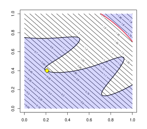
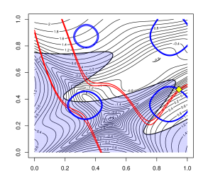
Figure 5: LSQ (left) and GSBP (right) problems. The contour lines show the objective functions, the bold lines the constraints, and the squares the solutions of the problems. Equality constraints are shown with two lines to represent the tolerance, the infeasible space defined by the inequality constraints are shaded.

References

- Adorio and Diliman, (2013) Adorio, E. and Diliman, U. (2013). “MVF: Multivariate Test Functions Library in C for Unconstrained Global Optimization.” Retrieved June 2013, from http://www.geocities.ws/eadorio/mvf.pdf.
- Audet and Dennis, Jr., (2006) Audet, C. and Dennis, Jr., J. (2006). “Mesh Adaptive Direct Search Algorithms for Constrained Optimization.” SIAM Journal on Optimization, 17, 1, 188–217.
- Audet and Dennis, Jr., (2009) — (2009). “A Progressive Barrier for Derivative-Free Nonlinear Programming.” SIAM Journal on Optimization, 20, 1, 445–472.
- Bäck, (1996) Bäck, T. (1996). Evolutionary algorithms in theory and practice: evolution strategies, evolutionary programming, genetic algorithms. Oxford University Press.
- Bertsekas, (1982) Bertsekas (1982). Constrained Optimization and Lagrange Multiplier Methods. New York, NY: Academic Press.
- Bingham et al., (2014) Bingham, D., Ranjan, P., and Welch, W. (2014). “Sequential design of computer experiments for optimization, estimating contours, and related objectives.” In Statistics in Action: A Canadian Outlook, ed. J. Lawless, 109–124. Chapman & Hall.
- Booker et al., (1999) Booker, A. J., Dennis, Jr., J. E., Frank, P. D., Serafani, D. B., Torczon, V., and Trosset, M. W. (1999). “A Rigorous Framework for Optimization of Expensive Functions by Surrogates.” Structural Optimization, 17, 1–13.
- Box and Draper, (1987) Box, G. E. P. and Draper, N. R. (1987). Empirical Model Building and Response Surfaces. Oxford: Wiley.
- Boyle, (2007) Boyle, P. (2007). “Gaussian Processes for Regression and Optimization.” Ph.D. thesis, Victoria University of Wellington.
- Brochu et al., (2010) Brochu, E., Cora, V. M., and de Freitas, N. (2010). “A Tutorial on Bayesian Optimization of Expensive Cost Functions, with Application to Active User Modeling and Hierarchical Reinforcement Learning.” Tech. rep., University of British Columbia. ArXiv:1012.2599v1.
- Bull, (2011) Bull, A. D. (2011). “Convergence Rates of Efficient Global Optimization Algorithms.” Journal of Machine Learning Research, 12, 2879–2904.
- Davies, (1980) Davies, R. (1980). “Algorithm AS 155: The Distribution of a Linear Combination of chi-2 Random Variables.” Journal of the Royal Statistical Society. Series C (Applied Statistics), 29, 3, 323–333.
- Dixon and Szego, (1978) Dixon, L. and Szego, G. (1978). “The global optimization problem: an introduction.” Towards global optimization, 2, 1–15.
- Duchesne and Lafaye de Micheaux, (2010) Duchesne, P. and Lafaye de Micheaux, P. (2010). “Computing the distribution of quadratic forms: Further comparisons between the Liu-Tang-Zhang approximation and exact methods.” Computational Statistics and Data Analysis, 54, 858–862.
- Forrester et al., (2008) Forrester, A., Sobester, A., and Keane, A. (2008). Engineering design via surrogate modelling: a practical guide. Wiley.
- Gardner et al., (2014) Gardner, J. R., Kusner, M. J., Xu, Z., Weinberger, K. W., and Cunningham, J. P. (2014). “Bayesian Optimization with Inequality Constraints.” In Proceedings of the 31st International Conference on Machine Learning, vol. 32. JMLR, W&CP.
- Gelbart et al., (2014) Gelbart, M. A., Snoek, J., and Adams, R. P. (2014). “Bayesian optimization with unknown constraints.” In Uncertainty in Artificial Intelligence (UAI).
- Ginsbourger et al., (2015) Ginsbourger, D., Picheny, V., Roustant, O., with contributions by C. Chevalier, Marmin, S., and Wagner, T. (2015). DiceOptim: Kriging-Based Optimization for Computer Experiments. R package version 1.5.
- Gramacy, (2015) Gramacy, R. (2015). “laGP: Large-Scale Spatial Modeling via Local Approximate Gaussian Processes in R.” Journal of Statistical Software, to appear. Available as a vignette in the laGP package.
- Gramacy et al., (2016a) Gramacy, R., Gray, G., Le Digabel, S., Lee, H., Ranjan, P., Wells, G., and Wild, S. (2016a). “Modeling an Augmented Lagrangian for Blackbox Constrained Optimization.” Technometrics, 58, 1–11.
- Gramacy et al., (2016b) — (2016b). “Rejoinder to Modeling an Augmented Lagrangian for Blackbox Constrained Optimization.” Technometrics, 58, 1, 26–29.
- Gramacy and Lee, (2011) Gramacy, R. B. and Lee, H. K. H. (2011). “Optimization under Unknown Constraints.” In Bayesian Statistics 9, eds. J. Bernardo, S. Bayarri, J. O. Berger, A. P. Dawid, D. Heckerman, A. F. M. Smith, and M. West, 229–256. Oxford University Press.
- Hernández-Lobato et al., (2015) Hernández-Lobato, J. M., Gelbart, M. A., Hoffman, M. W., Adams, R. P., and Ghahramani, Z. (2015). “Predictive Entropy Search for Bayesian Optimization with Unknown Constraints.” In Proceedings of the 32nd International Conference on Machine Learning, vol. 37. JMLR, W&CP.
- Johnson, (2014) Johnson, S. G. (2014). “The NLopt nonlinear-optimization package.” Via the R package nloptr.
- Jones et al., (1998) Jones, D. R., Schonlau, M., and Welch, W. J. (1998). “Efficient Global Optimization of Expensive Black Box Functions.” J. of Global Optimization, 13, 455–492.
- Lafaye de Micheaux, (2013) Lafaye de Micheaux, P. (2013). CompQuadForm: Distribution function of quadratic forms in normal variables. R package version 1.4-1.
- Le Digabel, (2011) Le Digabel, S. (2011). “Algorithm 909: NOMAD: Nonlinear Optimization with the MADS algorithm.” ACM Transactions on Mathematical Software, 37, 4, 44:1–44:15.
- Liu and Nocedal, (1989) Liu, D. C. and Nocedal, J. (1989). “On the limited memory BFGS method for large scale optimization.” Mathematical Programming, 45, 1-3, 503–528.
- Mebane Jr and Sekhon, (2011) Mebane Jr, W. R. and Sekhon, J. S. (2011). “Genetic optimization using derivatives: the rgenoud package for R.” Journal of Statistical Software, 42, 11, 1–26.
- Mockus, (1989) Mockus, J. (1989). Bayesian Approach to Global Optimization: Theory and Applications. Springer.
- Mockus, (1994) — (1994). “Application of Bayesian Approach to Numerical Methods of Global and Stochastic Optimization.” J. of Global Optimization, 4, 347–365.
- Mockus et al., (1978) Mockus, J., Tiesis, V., and Zilinskas, A. (1978). “The Application of Bayesian Methods for Seeking the Extremum.” Towards Global Optimization, 2, 117-129, 2.
- Molga and Smutnicki, (2005) Molga, M. and Smutnicki, C. (2005). “Test functions for optimization needs.” Retrieved June 2013, from http://www.zsd.ict.pwr.wroc.pl/files/docs/functions.pdf.
- Nocedal and Wright, (2006) Nocedal, J. and Wright, S. J. (2006). Numerical Optimization. 2nd ed. Springer.
- Parr et al., (2012) Parr, J., Keane, A., Forrester, A., and Holden, C. (2012). “Infill sampling criteria for surrogate-based optimization with constraint handling.” Engineering Optimization, 44, 1147–1166.
- Pav, (2015) Pav, S. E. (2015). sadists: Some Additional Distributions. R package version 0.2.1.
- Picheny, (2014) Picheny, V. (2014). “A stepwise uncertainty reduction approach to constrained global optimization.” In Proceedings of the 7th International Conference on Artificial Intelligence and Statistics, vol. 33, 787–795. JMLR W&CP.
- Picheny et al., (2016) Picheny, V., Ginsbourger, D., and Krityakierne, T. (2016). “Comment: Some Enhancements Over the Augmented Lagrangian Approach.” Technometrics, 58, 1, 17–21.
- Picheny et al., (2013) Picheny, V., Wagner, T., and Ginsbourger, D. (2013). “A benchmark of kriging-based infill criteria for noisy optimization.” Structural and Multidisciplinary Optimization, 48, 3, 607–626.
- Rasmussen and Williams, (2006) Rasmussen, C. E. and Williams, C. K. I. (2006). Gaussian Processes for Machine Learning. The MIT Press.
- Santner et al., (2003) Santner, T. J., Williams, B. J., and Notz, W. I. (2003). The Design and Analysis of Computer Experiments. New York: Springer-Verlag.
- Sasena, (2002) Sasena, M. J. (2002). “Flexibility and Efficiency Enhancement for Constrained Global Design Optimization with Kriging Approximations.” Ph.D. thesis, University of Michigan.
- Schonlau et al., (1998) Schonlau, M., Welch, W. J., and Jones, D. R. (1998). “Global versus local search in constrained optimization of computer models.” Lecture Notes-Monograph Series, 11–25.
- R Development Core Team, (2004) R Development Core Team (2004). R: A language and environment for statistical computing. R Foundation for Statistical Computing, Vienna, Aus. ISBN 3-900051-00-3.
- Snoek et al., (2012) Snoek, J., Larochelle, H., Snoek, J., and Adams, R. P. (2012). “Bayesian optimization of machine learning algorithms.” In Neural Information Processing Systems (NIPS).
- Surjanovic and Bingham, (2014) Surjanovic, S. and Bingham, D. (2014). “Virtual Library of Simulation Experiments: Test Functions and Datasets.” Retrieved December 4, 2014, from http://www.sfu.ca/~ssurjano.
- Williams et al., (2010) Williams, B. J., Santner, T. J., Notz, W. I., and Lehman, J. S. (2010). “Sequential Design of Computer Experiments for Constrained Optimization.” In Statistical Modeling and Regression Structures, eds. T. Kneib and G. Tutz, 449–472. Springer-Verlag.