Massive neutrinos in
nonlinear large scale structure:
A consistent perturbation theory

Abstract

A consistent formulation to incorporate massive neutrinos in the perturbation theory of the effective CDM+baryons fluid is introduced. In this formulation all linear k dependence in the growth functions of CDM+baryons perturbations, as well as all consequent additional mode coupling at higher orders, are taken into account to any desirable accuracy. Our formulation regards the neutrino fraction, which is constant in time after the non-relativistic transition of neutrinos, and much smaller than unity, as the coupling constant of the theory. Then the “bare” perturbations are those in the massless neutrino case when the neutrino fraction vanishes, and we consider the backreaction corrections due to the gravitational coupling of neutrinos. We derive the general equations for the “bare” perturbations, and backrecation corrections. Then, by employing exact time evolution with the proper analytic Green’s function we explicitly derive the leading backreaction effect, and find precise agreement at the linear level. We proceed to compute the second order beackreaction correction, and derive the leading order matter bispectrum in the presence of massive neutrinos, suggesting the squeezed limit of the matter bispectrum as a sensitive probe of neutrino mass. Notably, the generic neutrino fraction formulation in this work may be similarly applied for the consistent inclusion of massive neutrinos within any perturbative approach.

1 Introduction

Future large scale structure surveys, such as the Euclid mission [1, 2, 3], or ground-based LSST [4], are expected to be the next leading probe of cosmological information. Beyond addressing the puzzling cosmological questions of the accelerated expansion of the Universe, i.e. the nature of Dark Energy, or the primordial fluctuations in the early Universe, they aim to explore questions that extend to other fields of fundamental physics, such as the composition of Dark Matter and neutrinos beyond the Standard Model of particle physics, or tests of alternative theories of Gravity. The goal of these future surveys is to reach a 1% observational accuracy, thus requiring similar high precision theoretical modeling of the relevant observables.

In particular, cosmological data may enable us to fix the absolute neutrino mass scale, and the number of neutrino species. Whereas the total neutrino mass $M_{\nu}\equiv\sum_{i}m_{\nu,i}$, with $m_{\nu,i}$ the mass of each neutrino species, has a lower bound of $M_{\nu}>0.06$ eV coming from neutrino oscillation data [5], it is the combination of cosmological data from the cosmic microwave background (CMB) and large scale structure (LSS) observations, which currently provides the stringent upper bound to this quantity at $M_{\nu}<0.14$ eV [6, 7]. In fact, cosmological structure formation is quite sensitive to the neutrino mass, and even the smallest possible total neutrino mass in the currently bound range has an impact of at least 5% on the total matter power spectrum across nonlinear scales, where the neutrino effect is maximal. Hence, in turn, in order to extract more information from galaxy surveys to also fix all cosmological parameters with high precision, it is essential to improve our understanding of linear and nonlinear structure formation, allowing to increase the volume of related Fourier space in realistic massive neutrino cosmologies.

Specifically nonlinear higher order corrections to n-point functions, in particular the total matter power spectrum in the presence of massive neutrinos, has been studied both analytically using perturbation theories [8], e.g. in [9, 10, 11, 12, 13, 14], and with N-body simulations, e.g. in the more recent [15, 16]. The leading order bispectrum has also been approached analytically in [17]. All previous analytical work treat cold dark matter (CDM) combined with baryons as an ideal pressureless fluid, which reproduces the departure from linear theory in a very limited range of scales, even in the case of massless neutrinos, roughly $k\lesssim 0.1h\,Mpc^{-1}$ at $z=0$. The works [9, 12, 10, 17, 18], which are based on standard perturbation theory (SPT) [8] consider an Einstein de Sitter (EdS) Universe as the baseline cosmology, rather than handle the exact $\Lambda$CDM time evolution. Other works [11, 13, 14] rely on the time renormalization group (TRG) flow approach , where the perturbative (loop) order is not well-defined. Previous works have ignored the k dependence of linear growth functions of the CDM+baryons perturbations in the presence of massive neutrinos, and the additional consequent mode coupling at higher orders, or considered them in an incomplete manner. N-body simulations have obtained the total matter power spectrum at low redshifts up to the present $z=0$, and reach large $k$ modes in the fully non-linear regime up to $k\sim 10\,h\,Mpc^{-1}$. It should be stressed though that even if N-body simulations succeed in modeling nonlinear observables to high precision, they must be grounded in theory, which extends to the mildly nonlinear regime.

Most previous analytical and numerical works treated neutrinos as a linear perturbation, which acts as an external gravitational source. All past works, both in analytical methods, and N-body simulations, concluded that on the relevant scales, and considering the constraints on the total neutrino mass, the total nonlinear matter power spectrum and leading order bispectrum in massive neutrino cosmologies can be described at the 1% level by accounting for the nonlinear evolution of CDM perturbations alone, while adopting the linear approximation for the neutrino component. In [14] a fluid description was assumed for the neutrino component in order to evaluate its nonlinear evolution. However, on length scales smaller than the characteristic free streaming scale, $k_{FS}$, the fluid description formally leads to acoustic oscillations in the neutrino density contrast, which renders the fluid approach a poor description of the clustering behavior of the free-streaming dark matter (DM). Indeed, in [17], which also set out to evaluate the nonlinear evolution of the neutrino component and to examine the validity of the fluid approximation on the transitional length scales $k\sim k_{FS}$, especially at higher perturbative orders, an enhanced breakdown of the fluid approximation at the nonlinear level was found for the relevant neutrino mass range, as all relevant observable $k$ modes are greater than $k_{FS}$. Finally, we also note that some of the analytical methods [18, 17], as well as N-body simulations, are computationally intensive, and hence practically not favorable.

In this work we introduce a consistent formulation for the inclusion of massive neutrinos in the evolution of matter perturbations, such that all linear k dependence of the CDM+baryons perturbations, as well as all additional mode coupling at higher orders, are taken into account to any desirable accuracy. This is done using the fact that the linear neutrino component, can be represented to any desirable accuracy as a sum of separable functions of $k$, the scale factor $a$, and a generic $f_{\nu}$ dependence, with the required asymptotic behavior. Our formulation, is based on the fact that after the non-relativistic (NR) transition of the neutrinos, the neutrino fraction, $f_{\nu}$, is constant in time, and very small, particularly so in light of the current constrained range of total neutrino mass in eq. (2.2). Therefore $f_{\nu}$ is ideal for use as the coupling constant of the theory including massive neutrinos, and our formulation is made in terms of a generic $f_{\nu}$. This is obviously advantageous in order to explore the possible range of this parameter. Then the “bare” perturbations are those in the massless neutrino case when the neutrino fraction vanishes, and we consider the backreaction corrections due to the gravitational coupling of massive neutrinos. Further, our formulation resides within the general perturbative view of the CDM and baryons as an effective fluid [19, 20], that is within a well-defined perturbative theory, reaching a $1\%$ accuracy for small redshifts and larger k modes, i.e. beyond $k\simeq 0.1\,h\,Mpc^{-1}$, in the mildly non-linear regime. We stress though that the ingredients presented here are generic, and can equally be applied in other perturbative approaches. We employ here an exact time evolution, using the proper explicit analytic Green’s function similar to the $\Lambda$CDM baseline cosmology, common to all $f_{\nu}$ cosmologies after the NR transition of neutrinos, rather than resorting to uncontrolled EdS-like approximations. This is done while maintaining computational efficiency for practical use.

The outline of the paper is as follows. In section 2 we begin with reviewing basic neutrino physics, focusing in section 2.1 on their impact on structure formation. In section 3, we start by highlighting the main ingredients in our formulation, which focuses on the exact evolution of the CDM+baryons perturbations. In section 3.1 we introduce the “bare” and backreaction perturbations, derive their general equations, and show the required exact time evolution, using the proper explicit analytic Green’s function. Then in section 3.2 we explicitly derive the leading backreaction effect, and find precise agreement with the linear effect, and the linear total matter power spectrum. In section 3.3 we proceed to compute the second order backreaction correction, and derive the leading order matter bispectrum in the presence of massive neutrinos, where we explore the suppression effect in the shape dependence of the bispectrum. Further, in section 3.4 we discuss the relevance of an exact evaluation of the nonlinear neutrino perturbations for high precision nonlinear LSS in the presence of massive neutrinos. In section 4 we summarize our main conclusions. Finally, in appendix A we provide useful numerical approximations for possible efficient accurate numerical evaluations in higher orders, and in appendix B we provide the details of the realizations implemented in this work.

2 Neutrino Cosmology

Let us review basic neutrino physics in cosmology, in particular their role in structure formation [21, 22, 23]

Massive neutrinos are considered hot dark matter since they decouple as relativistic particles in the early Universe, just before the onset of Big Bang Nucleosynthesis. The mass density of the massive neutrinos after they have become non-relativistic is given by

$$\Omega_{\nu}h^{2}=\frac{M_{\nu}}{93.14\,eV}.$$ (2.1)

The current bounds on the sum of neutrino masses, which are not included in the Standard Model of particle physics, are given by

$$0.06\,eV\lesssim M_{\nu}\equiv\Sigma\,m_{\nu}\lesssim 0.14\,eV.$$ (2.2)

The lower bound comes from solar and atmospheric neutrino oscillation experiments [5], as discovered in 1998, whereas the most stringent upper bounds come from Cosmology, provided by constraints from the combination of recent CMB and LSS data [7, 6].

The ratio of the neutrino density to the total matter density, namely the neutrino fraction $f_{\nu}$, is given by

$$f_{\nu}\equiv\frac{\Omega_{\nu}}{\Omega_{m}}\lesssim 0.01,$$ (2.3)

and is constant once the neutrinos have become non-relativistic (NR). This fact, together with the smallness of $f_{\nu}$, play a key role in our ability to formulate a perturbation theory for the inclusion of massive neutrinos in structure formation, using $f_{\nu}$ as the small coupling constant of the theory, as we illustrate in section 3.

The massive neutrinos have a large velocity dispersion, $\sigma_{\nu}$, following their frozen Fermi-Dirac distribution since their decoupling. The non-relativistic transition of the neutrinos occurs when the mean neutrino energy becomes smaller than the neutrino mass, i.e.

$$\langle E\rangle=\frac{\int d^{3}p\,p\,[(exp(p/T_{\nu}(z))+1]^{-1}}{\int d^{3}p\,[(exp(p/T_{\nu}(z))+1]^{-1}}\simeq 3.15T_{\nu,0}(1+z)\leq m_{\nu},$$ (2.4)

hence at a redshift given by

$$1+z_{nr}\simeq\frac{m_{\nu}}{5.28\times 10^{-4}\,eV}.$$ (2.5)

After the non-relativistic transition the neutrino thermal velocity decays with time like

$$\sigma_{\nu}\simeq 150(1+z)\left[\frac{1\,eV}{m_{\nu}}\right]km\,s^{-1},$$ (2.6)

which is just the analogue of the cosmological redshift for a massive particle, and we note that the non-relativistic transition occurs when $\sigma_{\nu}\simeq 0.3\,c$, where $c$ is the speed of light.

2.1 Massive neutrinos and structure formation

If we write a fluid equation for the neutrino component, we get

$$\dot{\theta}(\vec{k},\tau)+\mathcal{H}(\tau)\theta(\vec{k},\tau)+\left(\frac{3}{2}\mathcal{H}^{2}(\tau)-k^{2}c_{s}^{2}(\tau)\right)\delta(\vec{k},\tau)=0,$$ (2.7)

where $\delta$ and $\theta$ denote the usual density contrast and velocity divergence, respectively. By analogy with the Jeans length, the neutrino velocity dispersion introduces a further time dependent dynamical scale into the problem, usually referred as the “free-streaming scale”, $\lambda_{FS}\equiv 2\pi ak_{FS}^{-1}$, which corresponds to the free-streaming wavenumber given by

$$k_{FS}(z)\equiv\sqrt{\frac{3}{2}}\frac{\mathcal{H}(z)}{c_{s}(z)}\simeq\sqrt{\frac{3}{2}}\frac{\mathcal{H}(z)}{\sigma_{\nu}(z)}.$$ (2.8)

This is the scale, below which collisionless particles cannot remain confined in gravitational potential wells, because of their velocity dispersion.

It should be noted that another integrated quantity is useful to describe the scale, above which neutrino free-streaming can be completely ignored. This is defined like any other comoving horizon scale:

$$d_{FS}(\eta)\equiv a(\eta)\int_{\eta_{dec}}^{\eta}\sigma_{\nu}(\eta)d\eta,$$ (2.9)

which we refer to as the “free-streaming horizon”. This gives the average distance traveled by neutrinos between the early universe and a given time. As long as the neutrinos are relativistic it is easy to see that the two scales are similar as the comoving free-streaming scale $k_{FS}^{-1}$ grows closely with the comoving Hubble scale $\mathcal{H}^{-1}$, until the non-relativistic transition of the neutrino.

However once the neutrino becomes non-relativistic the comoving free-streaming scale $k_{FS}^{-1}$ starts decreasing. Thus there is a maximal comoving free-streaming scale, corresponding to the wavenumber denoted by $k_{nr}$, which is set by the minimal value of $k_{FS}$ at the time of the non-relativistic transition. This scale is approximated by

$$k_{nr}\equiv k_{FS}(z_{nr})\simeq 0.018\sqrt{\Omega_{m}\left[\frac{m_{\nu}}{1\,eV}\right]}\,h\,Mpc^{-1}\lesssim 5\times 10^{-3}\,h\,Mpc^{-1}.$$ (2.10)

Hence, modes with $k\lesssim k_{nr}$ are not affected by free-streaming, and evolve like in a pure $\Lambda$CDM cosmology. Yet, all relevant observable $k$ modes are greater than $k_{nr}$.

Figure 1: The transition to a non-relativistic free streaming scale of a massive neutrino as a function of the scale factor, a, for the total neutrino mass values: $M_{\nu}=0.06,0.12,0.24$ eV, and 3 degenerate massive species. The black dotted line is the comoving horizon scale. The blue dotted line shows the free streaming horizon scale for $M_{\nu}=0.06$ eV after the NR transition at late times. The colored lines are approximations to the free streaming scale, $k_{FS}$, in the NR limit, which hold only after the NR transition time, roughly when the lines intersect with the comoving horizon scale. Lighter neutrinos become NR at later times, and in the NR limit the free streaming scale is just proportional to the neutrino mass, $k_{FS}\propto m_{\nu}$. The neutrino density fluctuations start to grow only when their modes enter the bluish region of the plot, e.g. for the $M_{\nu}=0.24$ eV case. Note that the relevant characteristic scale is in fact that, which corresponds the free streaming horizon. This scale still decreases with time, but remains close to $k_{nr}$, the minimal $k_{FS}$, after the NR transition. Hence, the characteristic free streaming scale is taken as $k_{nr}\simeq 5\times 10^{-3}$, notably below current observable scales.

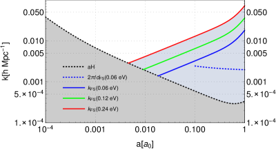
We note that the comoving free-streaming horizon $a^{-1}d_{FS}$ increases with time, but that for late times it remains very close to the maximal comoving free-streaming scale $2\pi k_{nr}^{-1}$. Actually, it is the comoving free streaming horizon, which is the strict scale to consider in order to know above which comoving scale free streaming can be completely neglected. However, in most of the literature it is $2\pi k_{nr}^{-1}$ that is considered, which makes no difference in practice for neutrinos becoming non-relativistic after the equality of matter and radiation. [21]. For this reason in this work we refer to $k_{nr}$ as the characteristic scale. In figure 1 we show the non-relativistic transition of the free streaming wavenumber $k_{FS}$, as inferred from the comoving Hubble horizon scale, and after the non-relativistic transition time from taking the non-relativistic limit approximation.

At wavenumbers $k\gtrsim k_{nr}$ the growth of CDM+baryons is suppressed due to the lack of neutrino perturbations, whereas at $k\lesssim k_{nr}$ the neutrinos cluster together with the CDM and baryons. Thus, the linear growth rate of CDM and baryons is scale dependent in the presence of massive neutrinos. Moreover, neutrino backreaction effects suppress the growth of matter perturbations. During matter domination on $k\gg k_{nr}$ the neutrino perturbations do not contribute to the gravitational clustering, although they do contribute to the homogeneous expansion. The linear suppression of the matter power spectrum with massive neutrinos with respect to that with massless neutrinos on scales below $k_{nr}$ is evaluated by

$$\frac{\Delta P_{L}^{f_{\nu}}}{P_{L}^{f_{\nu}=0}}\sim-8f_{\nu}\gtrsim 4\%.$$ (2.11)

Figure 2: Left: The linear matter power spectrum in the absence of neutrinos, and in the presence of massless and massive neutrinos with 3 degenerate species. The different solid lines correspond to total neutrino mass values $M_{\nu}=0,0.06,0.15,0.24$ eV, parametrized by the neutrino fraction $f_{\nu}=0,0.004,0.011,0.018$, respectively, where the baryon and total matter densities are fixed, and the neutrino and CDM densities are varied accordingly. Right: The suppression of linear matter power spectrum with massive neutrinos with respect to massless neutrinos. The notation is similar to that on the left figure. As expected the suppression grows with the total neutrino mass. The minimal wavenumber, where the suppression appears is located at $k_{nr}\sim 10^{-3}-10^{-2}$.

In figure 2 we show the linear suppression of the matter power spectrum for various values of the neutrino fraction, corresponding to the relevant mass range in eq. (2.2). The neutrino effect is maximal beyond the linear regime, and appears at very similar scales to BAOs. From N-body simulations [15, 16] the non-linear suppression of the matter power spectrum is evaluated to

$$\frac{\Delta P_{NL}^{f_{\nu}}}{P_{NL}^{f_{\nu}=0}}\sim-10f_{\nu}\gtrsim 5\%.$$ (2.12)

In terms of the total matter density contrast, which is given by

$$\delta^{m}=(1-f_{\nu})\delta^{c}+f_{\nu}\delta^{\nu},$$ (2.13)

where we denote by the superscript “c” the combined component of CDM and baryons, the total matter power spectrum, is given by

$$\langle\delta^{m}\delta^{m}\rangle=\left(1-f_{\nu}\right)^{2}\langle\delta^{c}\delta^{c}\rangle+2\left(1-f_{\nu}\right)f_{\nu}\langle\delta^{c}\delta^{\nu}\rangle+f_{\nu}^{2}\langle\delta^{\nu}\delta^{\nu}\rangle,$$ (2.14)

where $\langle\delta(\vec{k})\delta(\vec{k}^{\prime})\rangle\equiv(2\pi)^{3}\delta_{D}(\vec{k}+\vec{k}^{\prime})P(k)$. If the neutrinos did not induce a gravitational backreaction effect on the evolution of the metric and the other perturbations, then the maximal effect of the neutrino masses would be simply to cut the power spectrum by a factor $(1-f_{\nu})^{2}$ for $k\gg k_{nr}$. However, the presence of neutrinos actually modifies the evolution of the CDM and baryon density contrasts, such that the linear suppression factor is greatly enhanced from 2, roughly by a factor of 4, as noted in eq. (2.11). To conclude, as also confirmed by numerical simulations the ratio of the matter spectra in the massive and massless cases smoothly interpolates between 1 for $k<k_{nr}$, and a plateau for $k\gg k_{nr}$, as can be seen in the right panel of figure 2.

3 Perturbation theory with massive neutrinos

Our goal in this work is to formulate properly and consistently the inclusion of massive neutrinos in the evolution of matter perturbations.

We provide here such formulation using several ingredients. First, we note that after the non-relativistic transition of neutrinos, the neutrino fraction, $f_{\nu}$, is constant in time, and is very small, in particular in light of the current constrained range of total neutrino mass in eq. (2.2). Therefore $f_{\nu}$ is ideal for use as the coupling constant of the theory including massive neutrinos, and our formulation is made in terms of a generic $f_{\nu}$. This is obviously advantageous in order to explore the possible range of this parameter. We employ here an exact time evolution, using the proper explicit analytic Green’s function, common to all $f_{\nu}$ cosmologies, rather than resorting to EdS-like approximations. The time evolution can be evaluated directly in a simple, sufficiently accurate manner also in higher orders than in this work, see e.g. appendix A. We also use the fact that the linear neutrino component, can be represented to any desirable accuracy as a sum of separable functions of $k$, the scale factor $a$, and a generic $f_{\nu}$ dependence, with the proper asymptotic behavior. Finally, our formulation resides within the general perturbative framework of the CDM and baryons as an effective fluid [19, 20], reaching a $1\%$ accuracy for small redshifts and larger k modes, that is beyond $k\simeq 0.1\,h\,Mpc^{-1}$, in the mildly non-linear regime. Yet, the ingredients presented in this formulation are generic, and can be equally applied in any perturbation theory.

The massive neutrinos are coupled gravitationally to CDM and baryons, and the neutrino density contrast should then be specified. After the neutrinos have become fully non-relativistic it holds that $\delta^{\nu}\leq\delta^{c}$, with an equality at the limit $k\ll k_{nr}$, whereas at $k\gg k_{nr}$ we have $\delta^{\nu}\ll\delta^{c}$. Then the nonlinear neutrino component is evaluated here at each order using the approximation

$$\delta^{\nu}\simeq\left(\frac{\delta^{\nu}_{L}}{\delta^{c}_{L}}\right)\delta^{c},$$ (3.1)

which indeed maintains the required asymptotic behavior. This approximation takes into account the backreaction effects from non-linearities in the cold dark matter on the neutrinos. Yet, we also note that a common simple approximation is that the neutrino component remains linear throughout time, where indeed all past numerical and analytical work support this approximation for the 1% accuracy. In section 3.4 we examine the extent to which the inclusion of a nonlinear correction to the neutrino component actually affects the leading nonlinear result within the 1% precision.

3.1 The equations of backreaction correction

In view of the above setup we focus our attention now on the evolution of the effective CDM+baryons component.

Let us begin by writing the density contrast of the CDM+baryons component in the following form:

$$\delta^{c}\equiv\sum_{i=1}^{\infty}\delta_{i}+f_{\nu}\,\sum_{i=1}^{\infty}\tilde{\delta}_{i}\equiv\delta+f_{\nu}\,\tilde{\delta},$$ (3.2)

where we denoted $\delta\equiv\sum_{i=1}^{\infty}\delta_{i}$, and $\tilde{\delta}\equiv\sum_{i=1}^{\infty}\tilde{\delta}_{i}$. This can be regarded as a parametrization around $f_{\nu}=0$, where we reduce to the “bare” perturbation $\delta$ in the massless neutrino case, i.e. $\Lambda$CDM, and $\tilde{\delta}$ represents its backreaction correction with the coupling to massive neutrinos. Similarly, we rewrite the velocity divergence, $\theta^{c}\equiv\vec{\nabla}\cdot\vec{v}^{c}$, as

$$\theta^{c}\equiv\sum_{i=1}^{\infty}\theta_{i}+f_{\nu}\,\sum_{i=1}^{\infty}\tilde{\theta}_{i},$$ (3.3)

and for the neutrino component we just use the usual perturbative expansion $\delta^{\nu}\equiv\sum_{i=1}^{\infty}\delta^{\nu}_{i}$.

Let us write the Newtonian equations for subhorizon evolution of the CDM+baryons component:

$$\dot{\delta}_{c}+\frac{1}{a}\partial_{j}\left[(1+\delta_{c})v_{c}^{j}\right] =0,$$ (3.4)

$$\dot{v}_{c}^{i}+Hv_{c}^{i}+\frac{1}{a}v_{c}^{j}\partial_{j}v_{c}^{i}+\frac{1}{a}\partial^{i}\phi =-\frac{1}{a}c_{s}^{2}\partial^{i}\delta_{c},$$ (3.5)

$$\nabla^{2}\phi =\frac{3}{2}\frac{\Omega_{m}^{0}H_{0}^{2}}{a}\left[\left(1-f_{\nu}\right)\delta_{c}+f_{\nu}\delta_{\nu}\right],$$ (3.6)

where we have included only the leading EFT counterterm [20], although it will not play a role to the order we are considering in this work, and we note that in the Poisson equation the CDM+baryons source term is replaced by the total matter density contrast as in eq. (2.13), including the neutrino component.

Next, we substitute in eqs. (3.4), (3.5), the Poisson equation, and the decomposition of density contrast and velocity divergence from eqs. (3.2), (3.3), and we write the equations independent of $f_{\nu}$, and linear in $f_{\nu}$. Due to the smallness of $f_{\nu}$ higher orders can be neglected. After we Fourier transform the density and velocity fields, and assume that the vorticity vanishes, so that $\vec{v}(\vec{k},t)=-i\frac{\vec{k}}{k^{2}}\theta(\vec{k},t)$ we obtain, as expected, that the evolution equations independent of $f_{\nu}$, are just those of standard $\Lambda$CDM for the usual CDM+baryons component with massless neutrinos. These equations for $\delta(\vec{k},t)$ and $\theta(\vec{k},t)$ read:

$$a\dot{\delta}+\theta =-\frac{1}{(2\pi)^{3}}\int d^{3}p\left[\alpha(\vec{p},\vec{k}-\vec{p})\delta(\vec{k}-\vec{p})\theta\left(\vec{p}\right)\right],$$ (3.7)

$$a\dot{\theta}+aH\theta+\frac{3}{2}\frac{\Omega_{m}^{0}H_{0}^{2}}{a}\delta =-\frac{1}{(2\pi)^{3}}\int d^{3}p\left[\beta(\vec{p},\vec{k}-\vec{p})\theta(\vec{k}-\vec{p})\theta(\vec{p})\right]+c_{s}^{2}k^{2}\delta,$$ (3.8)

where

$$\alpha(\vec{p},\vec{q})=\frac{\left(\vec{p}+\vec{q}\right)\cdot\vec{p}}{p^{2}},\qquad\beta(\vec{p},\vec{q})=\frac{1}{2}\frac{\left(\vec{p}+\vec{q}\right)^{2}\vec{p}\cdot\vec{q}}{p^{2}q^{2}}.$$ (3.9)

Note that according to our definition in eq. (3.2) the linear solution here is expected to correspond to that obtained from a linear Boltzmann code [24, 25] for a massless neutrino cosmology. Further, the merit of this decomposition of the “bare” perturbations is that the linear growth functions of this component are still k independent at the linear level.

Proceeding to the equations linear in $f_{\nu}$ in a similar manner, we obtain the following equations for $\tilde{\delta}(\vec{k},t)$ and $\tilde{\theta}(\vec{k},t)$:

$$a\dot{\tilde{\delta}}+\tilde{\theta}=-\frac{1}{(2\pi)^{3}}\int d^{3}p\left[\alpha(\vec{p},\vec{k}-\vec{p})\left(\tilde{\delta}(\vec{k}-\vec{p})\theta\left(\vec{p}\right)+\delta(\vec{k}-\vec{p})\tilde{\theta}\left(\vec{p}\right)\right)\right],$$ (3.10)

$$a\dot{\tilde{\theta}}+aH\tilde{\theta}+\frac{3}{2}\frac{\Omega_{m}^{0}H_{0}^{2}}{a}\left(\tilde{\delta}+\delta^{\nu}-\delta\right)=-\frac{2}{(2\pi)^{3}}\int d^{3}p\left[\beta(\vec{p},\vec{k}-\vec{p})\theta(\vec{k}-\vec{p})\tilde{\theta}(\vec{p})\right]+c_{s}^{2}k^{2}\tilde{\delta}.$$ (3.11)

Notice the unique gravitational source term, which has an addition in terms of the difference of density components: since after the non-relativistic transition it holds that $\delta^{\nu}\leq\delta^{c}\leq\delta$, then we see that the free-streaming of massive neutrinos indeed gives rise to anti-Gravity for the CDM+baryons component, that is the backreaction correction, resulting the suppression of growth of CDM+baryons structure formation. Also note that due to this additional anti-Gravity source term, $\tilde{\delta}$ and $\tilde{\theta}$ have a “mixed” $k$ and time dependence already at the linear level, so that at higher orders the nonlinear convolution k integrals would actually be more complicated, even though they only contain the generic $\Lambda$CDM kernels from eq. (3.9) in the generic form. This is so since the $\delta^{\nu}$ component, which is a source in the linearized equations, has a non-trivial $k$ and time dependence.

We consider the evolution of these last equations as of an initial time after the non-relativistic transition, when even the lightest neutrinos have become non-relativistic, while the non-linearities are still small. Yet, for the standard “bare” CDM+baryons component in eqs. (3.7), by its definition (3.8) the initial time can be extended back to the onset of matter domination, or practically to 0.

As we noted, the linear form of these two sets of equations is similar up to the additional source term in the backreaction equations. Therefore, we resort to the Green’s function in order to solve them order by order. As in standard $\Lambda$CDM we have the following homogeneous linear ODE for the linear density contrasts, obtained from combining eqs. (3.7) and (3.8), and switching to the scale factor $a$ as the independent variable:

$$-a^{4}H^{2}\delta^{\prime\prime}-(3a^{3}H^{2}+a^{4}HH^{\prime})\delta^{\prime}+\frac{3}{2}\frac{\Omega_{m}^{0}H_{0}^{2}}{a}\delta=0.$$ (3.12)

The growing solution of this equation is given by

$$\delta_{1+}(a,\vec{k})=C\delta_{1}(\vec{k})H(a)\int_{0}^{a}dx\frac{1}{x^{3}H^{3}(x)},$$ (3.13)

where we define the linear growth function by $\delta_{1+}(\vec{k},a)\equiv D_{+}(a)\delta_{1}(\vec{k})$, and $C$ is the normalization constant we fix for the linear growth function, e.g. $C=\frac{5}{2}\Omega_{m}^{0}H_{0}^{2}$, or that for which $D(a_{0}=1)=1$, such that

$$D_{+}(a)=CH(a)\int_{0}^{a}dx\frac{1}{x^{3}H^{3}(x)}.$$ (3.14)

The decaying solution is given by $D_{-}(a)=H/H_{0}$. Then from eq. (3.7), we have

$$\theta_{1}(a,\vec{k})=-a^{2}H\delta_{1}^{\prime}(a,\vec{k})=-a^{2}HD^{\prime}_{+}(a)\delta_{1}(\vec{k}).$$ (3.15)

Yet, for the linear correction to the CDM+baryons density contrast we have a nonhomogeneous linear ODE due to the anti-Gravity source coming from the free streaming of massive neutrinos. From eqs. (3.10) and (3.11) we have:

$$-a^{4}H^{2}\tilde{\delta}^{\prime\prime}-(3a^{3}H^{2}+a^{4}HH^{\prime})\tilde{\delta}^{\prime}+\frac{3}{2}\frac{\Omega_{m}^{0}H_{0}^{2}}{a}\tilde{\delta}=\frac{3}{2}\frac{\Omega_{m}^{0}H_{0}^{2}}{a}\left(\delta-\delta^{\nu}\right).$$ (3.16)

It is essential then to have the Green’s function already at the linear level. We recall that the Green’s function should satisfy that

$$-a^{4}H^{2}(a)\partial^{2}_{a}G(a,\bar{a})-\left[3a^{3}H^{2}(a)+a^{4}H(a)H^{\prime}(a)\right]\partial_{a}G(a,\bar{a})+\frac{3}{2}\frac{\Omega_{m}^{0}H_{0}^{2}}{a}G(a,\bar{a})=\delta_{D}(a-\bar{a}),$$ (3.17)

and that it should hold that $G(a,\bar{a})=0$ for $a<\bar{a}$ with the boundary conditions on $a=\bar{a}$ being $G(a,\bar{a})|_{a=\bar{a}}=0$, and $\partial_{a}G(a,\bar{a})|_{a=\bar{a}}=-1/(\bar{a}^{4}H^{2}(\bar{a}))$. We find that the Green’s function is given by the following analytic closed form:

$$G(a,\bar{a})=\frac{H(a)}{\bar{a}}\int_{a}^{\bar{a}}dx\frac{1}{x^{3}H^{3}(x)}\,\theta_{H}(a-\bar{a}).$$ (3.18)

Let us stress that the Hubble parameter, which determines the Green’s function, corresponds to the total matter here, as in the massless neutrino case, and there is no distinction here between the CDM+baryons and the neutrino components since at this stage we consider the neutrino component to be non-relativistic, and thus its background density decays in time just as that of CDM+baryons. For this reason this Green’s function is common to all $f_{\nu}$ cosmologies. As the Green’s function plays a central role in our derivations, we provide an alternative efficient accurate evaluation of the Green’s function in appendix A for possible use in higher orders.

3.2 Leading order backreaction correction

The solution to eq. (3.16) of the initial value problem is given by

$$\tilde{\delta}_{1}(a,\vec{k})= \frac{3}{2}\Omega_{m}^{0}H_{0}^{2}\int_{a_{in}}^{a}d\bar{a}\,\frac{G(a,\bar{a})}{\bar{a}}\left[\delta_{1}(\bar{a},\vec{k})-\delta^{\nu}_{1}(\bar{a},\vec{k})\right]$$

$$+\tilde{\delta}_{in}(\vec{k})-\tilde{\delta}^{\prime}_{in}(\vec{k})a_{in}^{4}H^{2}(a_{in})G(a,a_{in}),$$ (3.19)

where we are considering the initial conditions:

$$\tilde{\delta}_{1}(a_{in},\vec{k})=\tilde{\delta}_{in}(\vec{k}),\qquad\partial_{a}\tilde{\delta}_{1}(a_{in},\vec{k})=\tilde{\delta}^{\prime}_{in}(\vec{k}).$$ (3.20)

and the latter is evaluated numerically from the Boltzmann code outputs.

For the velocity divergence we have

$$\tilde{\theta}_{1}(a,\vec{k})=-a^{2}H\left(\frac{3}{2}\Omega_{m}^{0}H_{0}^{2}\int_{a_{in}}^{a}d\bar{a}\,\frac{\partial_{a}G(a,\bar{a})}{\bar{a}}\left[\delta_{1}(\bar{a})-\delta^{\nu}_{1}(\bar{a})\right]-\tilde{\delta}^{\prime}_{in}a_{in}^{4}H^{2}(a_{in})\partial_{a}G(a,a_{in})\right).$$ (3.21)

In the evaluation of these solutions there are two main issues to consider. First, is the choice of initial time, $a_{in}$. We choose $a_{in}\gtrsim a_{nr}$ according to our consideration of the neutrino component becoming fully non-relativistic. We recall that this is in fact essential within our analysis here in terms of $f_{\nu}$ as our small coupling parameter, which is constant in time only once the neutrino component is fully non-relativistic. Yet, $a_{in}$ should also be smaller than $a_{NL}$, the time designating the onset of significant nonlinear structure formation. Past work on nonlinear structure formation with massive neutrinos contained a wide range of initial redshifts $z_{in}=99-9$. Yet, on $z=99$ e.g., 10% of the neutrinos are still relativistic, whereas on $z=9$ nonlinear effects are already non negligible. In this work we then specify to $z_{in}=24.12$ as the optimal initial time for structure formation with massive neutrinos, see also appendix B for further details of our realization.

Figure 3: The ratio of the linear neutrino component of a massive neutrino cosmology with $f_{\nu}=0.01291$ to the CDM+baryons component in the presence of massless neutrinos, and its high k asymptotic behavior.

Second, we recall that the neutrino component introduces a non-trivial “mixed” time and $k$ dependence to the source. Therefore, we would like to represent it as a sum of separable functions of time and $k$, specifically, in the following form:

$$\frac{\delta^{\nu}(a,\vec{k})}{\delta(a,\vec{k})}=\sum_{i=0}^{n}F_{i}(k;f_{\nu})\,a^{i},\quad n\in N$$ (3.22)

with as few terms as possible to a desirable accuracy. The expansion is done with monomials of the scale factor $a$, being the simplest generic time basis.

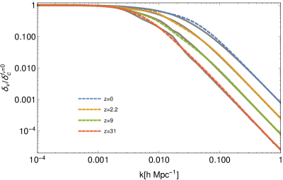
In figure 3 we see this ratio at various redshifts, where its asymptotic behavior is found to be

$$\frac{\delta^{\nu}(a,\vec{k})}{\delta(a,\vec{k})}\simeq\left\{\begin{array}[]{ll}1,&\quad k\ll k_{nr},\\ Af_{\nu}^{2}\,\dfrac{a}{k^{2}},&\quad k\gg k_{nr},\\ \end{array}\right.$$ (3.23)

with a constant A, and we see that the leading neutrino perturbation spans three orders of $f_{\nu}$ across the k domain. Hence, we postulate for $F_{i}(k;f_{\nu})$ a generic ansatz of the form of a fractional function of $k^{2}$, satisfying the leading asymptotic behavior, and make a fitting for the free parameters of the ansatz in the proper intermediate k domain, $\sim 10^{-3}-0.5\,h\,Mpc^{-1}$, using a standard least squares fitting procedure. We note that $f_{\nu}$ is easily incorporated as a parameter into the fitting, such that one gets a generic $f_{\nu}$ fitting, and in the following we suppress the dependence of the fitting coefficients $F_{i}$ on $f_{\nu}$. The fitting is shown for various redshifts in figure 4, where in this work three terms were included in the expansion in eq. (3.22), that is one additional term beyond the two necessary to satisfy the asymptotics in eq. (3.23), for a permille precision in the final results.

Figure 4: The fitting vs. CLASS data for the ratio of the linear neutrino component of a massive neutrino Cosmology with $f_{\nu}=0.01291$ to the CDM+baryons component in the presence of massless neutrinos. The fits at various redshifts are represented by colored dashed lines, corresponding to the CLASS data on the gray lines.

Therefore, with the fitting for the neutrino component in eq. (3.22) the linear solution in eq. (3.2) reads:

$$\tilde{\delta}_{1}(a,\vec{k})=\tilde{I}_{1,0}(a)\delta_{1}(\vec{k})[1-F_{0}(\vec{k})]-\tilde{I}_{1,j}(a)\delta_{1}(\vec{k})F_{j}(\vec{k})+\tilde{\delta}_{in}(\vec{k})-\tilde{\delta}^{\prime}_{in}(\vec{k})a_{in}^{4}H^{2}(a_{in})G(a,a_{in}),$$ (3.24)

where we denoted

$$\tilde{I}_{1,j}(a)=\frac{3}{2}\Omega_{m}^{0}H_{0}^{2}\int_{a_{in}}^{a}d\bar{a}\,G(a,\bar{a})D_{+}(\bar{a})\,\bar{a}^{j-1},$$ (3.25)

and a summation on the relevant j indices is implied.

Figure 5: The ratio of $\delta_{1}^{c}(a)$ computed from Green’s function, and with fitting of neutrino component, to that of CLASS data at k=0.1 h/Mpc in a massive neutrino Cosmology of $f_{\nu}=0.01291$.

Figure 6: The ratio of the linear power spectrum, $P_{L}$, computed from Green’s function, and with fitting of neutrino component, to that of CLASS data at $z=0$ in a massive neutrino Cosmology of $f_{\nu}=0.01291$. We note that CLASS data showed a 1% variance across the k domain, and no unique high precision settings to fix was possible for this version of the CLASS code (2.4.3).

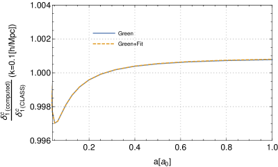
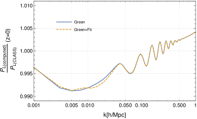
In figure 5 we show the ratio of the linear density contrast computed using eq. (3.2), and using eq. (3.24) with the fitting, to the that from the CLASS data, and we see an excellent agreement. Hence, the fitting allows us to include the additional k dependence entering already at the linear level in an analytic manner to any desirable accuracy, which we can then use in the higher order convolution integrals.

Next, let us consider the linear power spectrum in the presence of massive neutrinos. Due to the smallness of the neutrino fraction $f_{\nu}$, and since $\delta_{\nu}\leq\delta$, and $\tilde{\delta}$ is of the same order of magnitude as $\delta$, we can write

$$\delta_{1}^{m}\simeq\delta_{1}-f_{\nu}\left(\delta_{1}-\tilde{\delta}_{1}-\delta_{1}^{\nu}\right),$$ (3.26)

and consider the linear power spectrum to linear order in $f_{\nu}$ within the 1% precision, such that

$$\langle\delta_{1}^{m}\,\delta_{1}^{m}\rangle\simeq(1-2f_{\nu})\langle\delta_{1}^{c}\,\delta_{1}^{c}\rangle+2f_{\nu}\langle\delta_{1}^{c}\,\delta_{1}^{\nu}\rangle \simeq(1-2f_{\nu})\langle\delta_{1}\,\delta_{1}\rangle+\underbrace{2f_{\nu}\langle\delta_{1}\,\delta_{1}^{\nu}\rangle}_{\text{FS of $\nu$s}}+\underbrace{2f_{\nu}\langle\delta_{1}\,\tilde{\delta}_{1}\rangle}_{\text{BR of CDM}},$$ (3.27)

where $\langle\delta_{1}(z,\vec{k})\,\delta_{1}(z,\vec{k}^{\prime})\rangle\equiv(2\pi)^{3}\delta_{D}(\vec{k}+\vec{k}^{\prime})P_{L}^{f_{\nu}=0}(z,k)$. Note the cross term with the neutrino component, which vanishes at $k\gg k_{nr}$ due to the free streaming of neutrinos, and the cross term of the backreaction correction with the “bare” CDM+baryons perturbation, which represents the leading backreaction effect of CDM+baryons, giving rise to the enhanced suppression of the linear matter power spectrum in the presence of massive neutrinos. The leading backreaction effect of CDM+baryons, preceded by a $2f_{\nu}$ factor, explicitly reads

$$\frac{\langle\delta_{1}\,\tilde{\delta}_{1}\rangle}{\langle\delta_{1}\,\delta_{1}\rangle} =D^{-1}(a)\left[\frac{3}{2}\Omega_{m}^{0}H_{0}^{2}\int_{a_{in}}^{a}d\bar{a}\,\frac{G(a,\bar{a})}{\bar{a}}D(\bar{a})\left[1-\sum_{j=0}^{n}\bar{a}^{j}F_{j}(k)\right]\right.$$

$$\left.\qquad\qquad\quad+\frac{\tilde{\delta}_{i}(k)}{\delta_{1}(k)}-a_{i}^{4}H^{2}(a_{i})G(a,a_{i})\frac{\tilde{\delta}^{\prime}_{i}(k)}{\delta_{1}(k)}\right].$$ (3.28)

Figure 7: The relative effect of the leading CDM+baryons backreaction, computed from Green’s function with fitting of neutrino component, and that of CLASS data at $k=0.1hMpc^{-1}$ in a massive neutrino cosmology of $f_{\nu}=0.01291$.

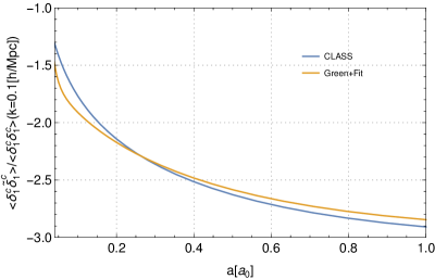
The linear power spectrum at $z=0$ obtained from our computation, and with the fitting, vs. that of the CLASS data is shown in figure 6, whereas the CDM+baryons relative backreaction effect at $k=0.1hMpc^{-1}$ is shown in figure 7. We can see from both figures that our computation is in very good agreement with the CLASS data.

3.3 Leading order matter bispectrum

For the second order backreaction correction we have to compute first the “bare” second order perturbation of CDM+baryons, $\delta_{2}$, and from eqs. (3.7), (3.8), we find

$$\delta_{2}(a,\vec{k})= -\frac{1}{(2\pi)^{3}}\int d^{3}p\,\delta_{1}(\vec{p})\delta_{1}(\vec{k}-\vec{p})$$

$$\qquad\qquad\qquad\times\left[I_{1}(a)\left(\alpha(\vec{p},\vec{k}-\vec{p})+\beta(\vec{p},\vec{k}-\vec{p})\right)+I_{2}(a)\alpha(\vec{p},\vec{k}-\vec{p})\right],$$ (3.29)

where we have

$$I_{1}(a)=\int_{a_{in}}^{a}d\bar{a}\,G(a,\bar{a})\bar{a}^{4}H^{2}(\bar{a})D_{+}^{{}^{\prime}2}(\bar{a}),$$ (3.30)

$$I_{2}(a)=\frac{3}{2}H_{0}^{2}\Omega_{m}^{0}\int_{a_{in}}^{a}d\bar{a}\,G(a,\bar{a})\frac{D_{+}^{2}(\bar{a})}{\bar{a}},$$ (3.31)

and where we consider the initial conditions:

$$\delta_{2}(a_{in}=0,\vec{k})=\delta_{2}^{in}(\vec{k})=0,\qquad\partial_{a}\delta_{2}(a_{in}=0,\vec{k})=\delta_{2}^{{}^{\prime}in}(\vec{k})=0,$$ (3.32)

and these are fixed at the initial time set at EdS, i.e. $a_{in}=a_{eq}\sim 10^{-4}\simeq 0$.

For the second order correction of the CDM+baryons perturbation with massive neutrinos, we obtain for eqs. (3.10), (3.11), the following solution:

$$\tilde{\delta}_{2}(a,\vec{k})= -\frac{1}{(2\pi)^{3}}\int d^{3}p\,\delta_{1}(\vec{p})\delta_{1}(\vec{k}-\vec{p})$$

$$\qquad\qquad\times\left[\left(\alpha(\vec{p},\vec{k}-\vec{p})+\beta(\vec{p},\vec{k}-\vec{p})\right)\left(\tilde{I}_{2,0}(a)[1-F_{0}(\vec{k})]-\tilde{I}_{2,j}(a)F_{j}(\vec{k})\right)\right.$$

$$\qquad\qquad\qquad+\alpha(\vec{p},\vec{k}-\vec{p})\left(\tilde{I}_{3,0}(a)[1-F_{0}(\vec{k})]-\tilde{I}_{3,j}(a)F_{j}(\vec{k})\right)$$

$$\qquad\qquad\quad+\left(\alpha(\vec{p},\vec{k}-\vec{p})+\alpha(\vec{k}-\vec{p},\vec{p})+2\beta(\vec{p},\vec{k}-\vec{p})\right)\times$$

$$\qquad\qquad\qquad\left(\tilde{I}_{4,0}(a)[1-F_{0}(\vec{p})]-\tilde{I}_{4,j}(a)F_{j}(\vec{p})-\tilde{I}_{5}(a)\frac{\tilde{\delta}^{\prime}_{in}(\vec{p})}{\delta_{1}(\vec{p})}\right)$$

$$\qquad\qquad\quad+\left(\alpha(\vec{p},\vec{k}-\vec{p})+\alpha(\vec{k}-\vec{p},\vec{p})\right)\times$$

$$\qquad\qquad\qquad\left(I_{6,0}(a)[1-F_{0}(\vec{p})]-\tilde{I}_{6,j}(a)F_{j}(\vec{p})+\tilde{I}_{1,0}(a)\frac{\tilde{\delta}_{in}(\vec{p})}{\delta_{1}(\vec{p})}-\tilde{I}_{7}(a)\frac{\tilde{\delta}^{\prime}_{in}(\vec{p})}{\delta_{1}(\vec{p})}\right)$$

$$\qquad\qquad\quad\left.-\alpha(\vec{p},\vec{k}-\vec{p})\left(\tilde{I}_{1,1}(a)[1-F_{0}(\vec{p})]-\tilde{I}_{1,j+1}(a)F_{j}(\vec{p})\right)\right],$$ (3.33)

where summation over the proper j indices is implied, and we have

$$\tilde{I}_{2,j}(a)= \frac{3}{2}\Omega_{m}^{0}H_{0}^{2}\int_{a_{in}}^{a}d\bar{a}\,G(a,\bar{a})\,\bar{a}^{j-1}I_{1}(\bar{a}),$$ (3.34)

$$\tilde{I}_{3,j}(a)= \frac{3}{2}\Omega_{m}^{0}H_{0}^{2}\int_{a_{in}}^{a}d\bar{a}\,G(a,\bar{a})\,\bar{a}^{j-1}I_{2}(\bar{a}),$$ (3.35)

$$\tilde{I}_{4,j}(a)= \frac{3}{2}\Omega_{m}^{0}H_{0}^{2}\int_{a_{in}}^{a}d\bar{a}\,G(a,\bar{a})\bar{a}^{4}H^{2}(\bar{a})D^{\prime}_{+}(\bar{a})\int_{a_{in}}^{\bar{a}}d\hat{a}\,\partial_{\bar{a}}G(\bar{a},\hat{a})D_{+}(\hat{a})\,\hat{a}^{j-1},$$ (3.36)

$$\tilde{I}_{5}(a)= a_{in}^{4}H^{2}(a_{in})\int_{a_{in}}^{a}d\bar{a}\,G(a,\bar{a})\bar{a}^{4}H^{2}(\bar{a})D^{\prime}_{+}(\bar{a})\partial_{\bar{a}}G(\bar{a},a_{in}),$$ (3.37)

$$\tilde{I}_{6,j}(a)= \frac{3}{2}\Omega_{m}^{0}H_{0}^{2}\int_{a_{in}}^{a}d\bar{a}\,G(a,\bar{a})\frac{D_{+}(\bar{a})}{\bar{a}}\tilde{I}_{1,j}(\bar{a}),$$ (3.38)

$$\tilde{I}_{7}(a)= \frac{3}{2}\Omega_{m}^{0}H_{0}^{2}\,a_{in}^{4}H^{2}(a_{in})\int_{a_{in}}^{a}d\bar{a}\,G(a,\bar{a})\frac{D_{+}(\bar{a})}{\bar{a}}G(\bar{a},a_{in}),$$ (3.39)

and where we consider the initial conditions:

$$\tilde{\delta}_{2}(a_{in},\vec{k})=\tilde{\delta}_{2}^{i}(\vec{k})=0,\qquad\partial_{a}\tilde{\delta}_{2}(a_{in},\vec{k})=\tilde{\delta}_{2}^{{}^{\prime}i}(\vec{k})=0,$$ (3.40)

and these are fixed at the initial time $a_{in}$, when we consider that the neutrinos only start to affect the nonlinear structure formation. Note that here we have used the approximation in eq. (3.1) for the second order neutrino component.

Let us then consider the LO matter bispectrum in the presence of massive neutrinos. We recall that the bispectrum is defined as

$$\langle\delta^{m}(\vec{k}_{1},z)\,\delta^{m}(\vec{k}_{2},z)\,\delta^{m}(\vec{k}_{3},z)\rangle\equiv(2\pi)^{3}\delta_{D}(\vec{k}_{1}+\vec{k}_{2}+\vec{k}_{3})B(\vec{k}_{1},\vec{k}_{2},\vec{k}_{3},z).$$ (3.41)

For the total matter bispectrum we then find, using eqs. (2.13), and (3.2), and dropping $f_{\nu}$ beyond linear order within the 1% precision

$$\langle\delta^{m}(\vec{k}_{1})\,\delta^{m}(\vec{k}_{2})\,\delta^{m}(\vec{k}_{3})\rangle\simeq \langle\delta^{c}(\vec{k}_{1})\,\delta^{c}(\vec{k}_{2})\,\delta^{c}(\vec{k}_{3})\rangle-f_{\nu}\left[3\langle\delta^{c}(\vec{k}_{1})\,\delta^{c}(\vec{k}_{2})\,\delta^{c}(\vec{k}_{3})\rangle\right.$$

$$\left.-\left(\langle\delta^{\nu}(\vec{k}_{1})\,\delta^{c}(\vec{k}_{2})\,\delta^{c}(\vec{k}_{3})\rangle+2\,\,\text{cyc.~{}perm.}\right)\right]$$

$$\simeq\langle\delta(\vec{k}_{1})\,\delta(\vec{k}_{2})\,\delta(\vec{k}_{3})\rangle-f_{\nu}\left[3\langle\delta(\vec{k}_{1})\,\delta(\vec{k}_{2})\,\delta(\vec{k}_{3})\rangle\right.$$

$$-\left(\langle\delta^{\nu}(\vec{k}_{1})\,\delta(\vec{k}_{2})\,\delta(\vec{k}_{3})\rangle+2\,\,\text{cyc.~{}perm.}\right)$$

$$\left.-\underbrace{\left(\langle\tilde{\delta}(\vec{k}_{1})\,\delta(\vec{k}_{2})\,\delta(\vec{k}_{3})\rangle+2\,\,\text{cyc.~{}perm.}\right)}_{\text{backreaction}}\right].$$ (3.42)

The first non-trivial contribution stems from the first nonlinear correction to $\delta_{1}^{m}$, i.e. $\delta_{2}^{m}$, which yields the tree level bispectrum, with the term that reads:

$$\langle \delta_{1}^{m}(\vec{k}_{1})\,\delta_{1}^{m}(\vec{k}_{2})\,\delta_{2}^{m}(\vec{k}_{3})\rangle\simeq\langle\delta_{1}(\vec{k}_{1})\,\delta_{1}(\vec{k}_{2})\,\delta_{2}(\vec{k}_{3})\rangle\left(1-3f_{\nu}\right)$$

$$+f_{\nu}\left(\langle\delta_{1}^{\nu}(\vec{k}_{1})\,\delta_{1}(\vec{k}_{2})\,\delta_{2}(\vec{k}_{3})\rangle+\langle\delta_{1}(\vec{k}_{1})\,\delta_{1}^{\nu}(\vec{k}_{2})\,\delta_{2}(\vec{k}_{3})\rangle+\frac{\delta_{1}^{\nu}(k_{3})}{\delta_{1}(k_{3})}\langle\delta_{1}(\vec{k}_{1})\,\delta_{1}(\vec{k}_{2})\,\delta_{2}(\vec{k}_{3})\rangle\right)$$

$$+f_{\nu}\left(\langle\tilde{\delta}_{1}(\vec{k}_{1})\,\delta_{1}(\vec{k}_{2})\,\delta_{2}(\vec{k}_{3})\rangle+\langle\delta_{1}(\vec{k}_{1})\,\tilde{\delta}_{1}(\vec{k}_{2})\,\delta_{2}(\vec{k}_{3})\rangle+\langle\delta_{1}(\vec{k}_{1})\,\delta_{1}(\vec{k}_{2})\,\tilde{\delta}_{2}(\vec{k}_{3})\rangle\right),$$ (3.43)

and we have made use of the approximation in eq. (3.1) to evaluate the term with the second order neutrino perturbation, such that:

$$\langle\delta_{1}^{c}(\vec{k}_{1})\,\delta_{1}^{c}(\vec{k}_{2})\,\delta_{2}^{\nu}(\vec{k}_{3})\rangle=\langle\delta_{1}^{c}(\vec{k}_{1})\,\delta_{1}^{c}(\vec{k}_{2})\,\delta_{2}^{c}(\vec{k}_{3})\rangle\frac{\delta_{1}^{\nu}(k_{3})}{\delta_{1}^{c}(k_{3})},$$ (3.44)

and dropped higher orders in $f_{\nu}$. Notice that the first two terms with the linear neutrino component in eq. (3.3) can then be brought to a similar form, of the massless neutrino bispectrum times the ratio of neutrino to CDM components.

Figure 8: The ratio of LO matter bispectra with $f_{\nu}=0.01291$ to $f_{\nu}=0$ at $z=0$ of three special configurations. The squeezed limit configuration shows a significant suppression at high k modes, suggesting the squeezed limit as a sensitive probe of neutrino mass.

We recall that the LO bispectrum in EdS reads:

$$B_{LO}^{EdS}(\vec{k}_{1},\vec{k}_{2},\vec{k}_{3},z)= \left(\frac{5}{7}\left[\alpha(\vec{k_{1}},\vec{k_{2}})+\alpha(\vec{k_{2}},\vec{k_{1}})\right]+\frac{4}{7}\beta(\vec{k_{1}},\vec{k_{2}})\right)P_{L}(k_{1},z)P_{L}(k_{2},z)$$

$$+2\,\,\text{cyc.~{}perm.},$$ (3.45)

and for $\Lambda$CDM, or the massless neutrino case, we get from eq. (3.3) that the LO bispectrum reads:

$$B_{LO}^{f_{\nu}=0}(\vec{k}_{1},\vec{k}_{2},\vec{k}_{3},z)= -\left(\frac{I_{1}(a)}{D^{2}_{+}(a)}\left[\alpha(\vec{k_{1}},\vec{k_{2}})+\alpha(\vec{k_{2}},\vec{k_{1}})+2\beta(\vec{k_{1}},\vec{k_{2}})\right]\right.$$

$$\left.\quad+\frac{I_{2}(a)}{D^{2}_{+}(a)}\left[\alpha(\vec{k_{1}},\vec{k_{2}})+\alpha(\vec{k_{2}},\vec{k_{1}})\right]\right)P_{L}(k_{1},z)P_{L}(k_{2},z)$$

$$+2\,\,\text{cyc.~{}perm.}$$ (3.46)

In order to explore the shape dependence of the bispectrum a reduced bispectrum can be defined as

$$Q=\frac{B(\vec{k_{1}},\vec{k_{2}},\vec{k_{3}})}{P_{L}(k_{1})P_{L}(k_{2})+P_{L}(k_{2})P_{L}(k_{3})+P_{L}(k_{3})P_{L}(k_{1})}.$$ (3.47)

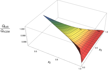
We then consider $Q$ for a fixed $k_{1}$ as a function of $x_{2}=k_{2}/k_{1}$ and $x_{3}=k_{3}/k_{1}$, which are constrained to $x_{2}\geq x_{3}\geq 1-x_{2}$. We show the ratio of reduced bispectra of EdS and $\Lambda$CDM in figure 12 in appendix A.

Figure 9: The ratio of LO matter bispectra with $f_{\nu}=0.01291$ to $f_{\nu}=0$ at $z=0$. We consider the shape dependence for a fixed $k_{1}=0.2\,h\,Mpc^{-1}$ as a function of $x_{2}=k_{2}/k_{1}$ and $x_{3}=k_{3}/k_{1}$, which are constrained to $x_{2}\geq x_{3}\geq 1-x_{2}$. The shape dependence shows a suppression of similar values to the equilateral configuration suppression of $\sim-13.5f_{\nu}$ , whereas a steep enhanced suppression appears around the squeezed limit at high k modes.

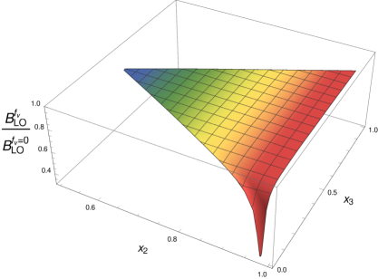
We examine here the particular cases of equilateral configuration, i.e. $k_{1}=k_{2}=k_{3}$, the triangle configuration given by $k_{2}/k_{1}=k_{3}/k_{1}=2$, and the squeezed limit, i.e. $k_{1}\to 0$, $k_{2}/k_{3}=1$. These bispectra are seen in figure 8. The tree level bispectrum should be similar to SPT extensions as in [17], since there are still no counterterms contributing at this perturbative order. For the equilateral configuration we find that the suppression of the LO bispectrum in the presence of massive neutrinos is given by

$$\frac{\Delta B_{LO}^{f_{\nu}}(k,k,k)}{B_{LO}^{f_{\nu}=0}(k,k,k)}\simeq-13.5\,f_{\nu},$$ (3.48)

in analogy to eq. (2.11) for the suppression of the linear power spectrum. Hence, the suppression effect that we find here is slightly larger than that estimated in [17], which started the evolution at a notably late redshift, where nonlinear effects cannot be neglected. The reduced bispectrum for a fixed $k_{1}=0.2\,h\,Mpc^{-1}$ is seen in figure 9, where we see that the shape dependence shows a suppression of similar values to the equilateral configuration suppression of $\sim-13.5f_{\nu}$ , whereas a steep enhanced suppression appears around the squeezed limit at high k modes.

3.4 Relevance of exact evaluation of nonlinear neutrino perturbation

Let us reconsider now the relevance of the exact evaluation of the nonlinear neutrino perturbation for the desirable 1% precision in nonlinear perturbation theory with massive neutrinos. We recall that in this work we have used for the nonlinear neutrino perturbation the evaluation given by eq. (3.1). This is in fact an upper bound for the exact NL value, since the NL clustering of neutrinos is expected to be even more suppressed, compared to that of CDM+baryons, than their relative linear clustering. On the other hand, an extremely crude lower bound would be just to take the nonlinear neutrino perturbation to vanish. Hence, the actual exact nonlinear neutrino perturbation is found in the following possible crude range

$$0<\delta_{NL}^{\nu}\lesssim\left(\frac{\delta^{\nu}_{L}}{\delta^{c}_{L}}\right)\delta^{c}_{NL},$$ (3.49)

and therefore an overly critical way to examine the importance of the exact evaluation of the nonlinear neutrino perturbation, would be to compare the results we would have obtained by taking the extreme lower bound, that is by assuming the nonlinear neutrino perturbation vanishes, and compare them with our results. We note that in this work the NL neutrino perturbation enters the final result from two origins: First in the anti-Gravity source for the NL CDM+baryons backreaction correction, i.e. in eq. (3.3). Second, explicitly in the bispectrum cross correlation of neutrino with CDM+baryons in eq.  (3.44). The results of this check can be seen in figure 10. We can see that even the extreme range of possible values for the exact nonlinear neutrino perturbation leads to a range of results, which is within the 1% precision for practically all observable scales.

Figure 10: The ratio of LO matter bispectra with $f_{\nu}=0.01291$, and $\delta_{2}^{\nu}=0$ to the bispectra computed in this work, using eq. (3.1), at $z=0$. We can see that even a wider range of possible values for the exact nonlinear neutrino perturbation leads to a range of results, which is within the 1% precision for practically all observable scales.

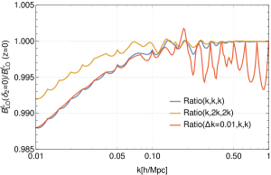
For completeness we note previous approaches to estimate the effect of the nonlinear neutrino perturbation on nonlinear results. In [9, 12] the neutrino perturbations were numerically approximated by solving the modified linearized Boltzmann equation, using the Boltzmann code CAMB [24], via plugging into the Poisson equation approximations of the NL density contrasts of CDM+baryons. The effect of this estimate was found there well below the 1% precision, and hence the linear neutrino assumption was adopted. In [14] the nonlinear neutrino perturbation was evaluated by treating the neutrino component as a fluid. Yet, as we already stressed above, this provides a poor description for the free streaming neutrino component on all relevant observable scales, which are larger than the characteristic free streaming scale. Finally, other approaches to evaluate the nonlinear neutrino component were put forward in [18], which requires the explicit evaluation of the perturbed neutrino momentum distribution in real time, and in [17], which is also computationally intensive, making both approaches impractical. As our results in figure 10 illustrate, along with similar conclusions of all previous analytical and numerical studies of NL observables with massive neutrinos, the exact evaluation of the NL neutrino perturbation, has negligible impact on the final results, at least up to the two-loop level, and therefore does not constitute a crucial aspect in evaluating successfully to 1% precision NL LSS with massive neutrinos. It is rather the exact evaluation of the CDM+baryons perturbations, and their backreaction corrections, as is realized in this work.

4 Conclusions

In this paper we introduced a consistent formulation for a perturbation theory that incorporates massive neutrinos in the evolution of matter perturbations, such that all linear k dependence in the growth functions of CDM+baryons perturbations, as well as all consequent additional mode coupling at higher orders are taken into account to any desirable accuracy. This is achieved using the fact that the linear neutrino perturbation, can be represented to any desirable accuracy as a sum of separable functions of $k$, the scale factor $a$, and a generic $f_{\nu}$ dependence, with the proper asymptotic behavior. Our formulation is based on that after the non-relativistic transition of the neutrinos, the neutrino fraction, $f_{\nu}$, is constant in time, and much smaller than unity, in particular in light of the current constraints on the total neutrino mass. Therefore, $f_{\nu}$ is regarded as the coupling constant of the theory including massive neutrinos, and our formulation is made in terms of a generic $f_{\nu}$, which is clearly advantageous for exploring the possible range of this particle physics parameter. Then the “bare” perturbations are those in the massless neutrino case when the neutrino fraction vanishes, and we consider the backreaction corrections due to the gravitational coupling of massive neutrinos. This also allows to consider the “bare” perturbations nonlinearities from an earlier redshift than their backreaction corrections, and hence capture dominant nonlinear effects, which occur before neutrinos become fully non-relativistic.

We have derived the general equations for the “bare” perturbations and their backreaction corrections, and carried out the exact time evolution, using the proper explicit analytic Green’s function, common to all $f_{\nu}$ cosmologies. We explicitly derived the leading backreaction effect, and found precise agreement with the linear effect, and the linear total matter power spectrum. Furthermore, we computed the second order backreaction correction, and derived the leading order matter bispectrum in the presence of massive neutrinos, suggesting that the squeezed limit of the LO matter bispectrum as a sensitive probe of neutrino mass. Finally, we have also demonstrated the irrelevance of the exact evaluation of the nonlinear neutrino perturbation for the 1% precision of our NL result in agreement with the conclusions of all previous studies of NL LSS with massive neutrinos.

Our perturbation theory resides within the general view of the CDM and baryons as an effective fluid, and is therefore well-defined, extending to a larger k reach in the mildly non-linear regime. Yet the generic formulation in this work allows for the consistent inclusion of massive neutrinos within any perturbative theory. We have employed an exact time evolution, using the analytic Green’s function similar to that of the baseline $\Lambda$CDM cosmology. Thus we refrained from resorting to EdS-like approximations, while still maintaining computational efficiency for practical use. The relevance of the exact time evolution for sub-percent precision calculations has also been recently investigated in [26], where it has been pointed out that these EdS-like approximations are less suited for higher order velocity statistics, relevant to all observables affected by redshift space distortion effects.

In this respect the only practical challenge in our formulation, that has to be tackled at higher orders, is the multiple time integrations, increasing with each order of the perturbative theory. For this purpose the generic time integrals of the Green’s function with powers of the scale factor should be considered for a possible analytical and useful accurate numerical simplification, such as those noted in appendix A. Further, the time integrations may be numerically implemented in non-trivial ways for more efficient evaluation. Finally, we note that external robust integration routines such as the CUBA library [27] may also be very useful to increase the efficient evaluation performance. We leave it for future work to extend the implementation of our formulation to higher orders of n point functions, and to be confronted with N-body simulations.

Appendix A Useful numerical approximations

For $\Lambda$CDM the growth function given in (3.14) can be approximated to 1 permille precision, using the function given by [8]

$$D_{+}(a)\simeq Nd(a)=N\,\frac{a\Omega_{m}}{\Omega_{m}^{4/7}-\Omega_{\Lambda}+\left(1+\frac{\Omega_{m}}{2}\right)\left(1+\frac{\Omega_{\Lambda}}{70}\right)},$$ (A.1)

where N is the proper normalization constant. This approximation is shown in figure 11.

The Green’s function in eq. (3.18) can be written directly in terms of the growth factor and the Hubble parameter as follows:

$$G(a,\bar{a})=C^{-1}\frac{D_{+}(\bar{a})}{\bar{a}}\left(\frac{D_{-}(a)}{D_{-}(\bar{a})}-\frac{D_{+}(a)}{D_{+}(\bar{a})}\right)\,\theta_{H}(a-\bar{a}),$$ (A.2)

where $C$ is the normalization constant of the growth factor from eq. (3.14), and hence eq. (A.1) can also be used in the Green’s function for an efficient numerical evaluation, rather than numerically evaluating the time integral in eq. (3.18).

Figure 11: Left: The ratios of the EdS approximation and of the approximation in (A.1) to the linear growth function $D_{+}$. Right: The ratios of the EdS-like approximation in eq. (A.3) to the time integrals, appearing in the second order density perturbation in $\Lambda$CDM.

The time integrals from eqs. (3.30), (3.31), appearing in the second order standard $\Lambda$CDM density perturbation in eq. (3.3), and consequently in the $\Lambda$CDM bispectrum in eq. (3.3) can be approximated within the 1% precision by their EdS-like value, that is

$$I_{1}(a)\simeq I_{2}(a)\simeq-\frac{2}{7}D_{+}^{2}(a),$$ (A.3)

as can be seen in figure 11. The effect of using this EdS-like approximation in the LO bispectrum of $\Lambda$CDM is shown in figure 12.

We should stress though that none of these approximations was employed in this work, where the exact computations were still very manageable.

Figure 12: The ratio of the reduced bispectra of the EdS-like approximation to $\Lambda$CDM, demonstrating the 1% precision attained, using the EdS-like approximation in eq. (A.3), rather than the exact Green’s time integral. The reduced bispectra are presented for a fixed $k_{1}=0.2\,h\,Mpc^{-1}$ as a function of $x_{2}=k_{2}/k_{1}$ and $x_{3}=k_{3}/k_{1}$, which are constrained to $x_{2}\geq x_{3}\geq 1-x_{2}$.

Appendix B Realization

In this work we have used the recent Boltzmann C code CLASS (version 2.4.3) [28, 25] to set up the initial conditions, e.g. to compute the input transfer functions for the CDM, baryons, and neutrino components in the massless and massive cases. CLASS seems to be better suited for the inclusion of massive neutrinos, which is implemented differently than in the commonly used CAMB code [29].

The main input parameters which were used for all neutrino cosmologies, following Planck 2013 [7], are noted in table 1. Additional input parameters which were used for all cosmologies are: Photon density $T_{\text{cmb}}=2.726$, primordial Helium fraction $YHe=0.25$, pivot scale in $Mpc^{-1}$ $k_{pivot}=0.05$, and tilt running $\alpha_{s}=0$. The input parameters, which varied among the neutrino cosmologies, in particular between the massless and massive cases, appear in table 2. For the massive case we considered a single distinct species with 3 degenerate massive neutrinos.

h	$\Omega_{m}$	$\Omega_{b}$	$A_{s}$	$n_{s}$
0.67	0.3167	0.05	2.1265$\times 10^{-9}$	0.96

Table 1: The cosmological parameters used in our massless and massive neutrino realizations.

$M_{\nu}$[eV]	$f_{\nu}$	$\Omega_{\text{cdm}}$	$N_{\textbf{eff}}$	$N_{ncdm}$
0.0	0	0.2667	3.04	—
0.06	4.531$\times 10^{-3}$	0.2653	0.0	1
0.102	7.703$\times 10^{-3}$	0.2643	0.0	1
0.141	1.065$\times 10^{-2}$	0.2633	0.0	1
0.171	1.291$\times 10^{-2}$	0.2626	0.0	1

Table 2: The various neutrino cosmologies parameters used in our realizations.

We output the matter transfer functions. In particular, we get the density contrast for each non-degenerate non-CDM species, hence in our case we get one value, and we consider the neutrino density fixed and distributed equally amongst three massive neutrino degenerate species.

The k domain of output in units of $h\,Mpc^{-1}$ is $\sim 10^{-5}-10^{3}$, and we took 15 uniform log intervals of redshifts, such that $Log[1+z]=0,..,1.4$, corresponding to the redshifts $z=$0, 0.26, 0.58, 1.00, 1.51, 2.16, 2.98, 4.01, 5.31, 6.94, 9.00, 11.59, 14.85, 18.95, 24.12.

Finally, we note that no unique high precision settings was possible for this version of the CLASS code.